Design of Positioning Mechanism Fit Clearances Based on On-Orbit Re-Orientation Accuracy

Featured Application

The research in this paper will be helpful to researchers studying the positioning mechanism of the on-orbit replaceable optical unit, and can provide them with a simple fit clearance design method. It can also assist with research on the re-orientation accuracy of the on-orbit replaceable unit and the design of fit clearance.

Abstract

The factors affecting the re-orientation accuracy of the on-orbit replaceable optical unit were studied, and the mathematical models of the relationships between fit clearances of positioning mechanisms and the limits of rotation angles were deduced. When the relative position relationship of positioning mechanisms was determined, fit clearances were designed according to the requirement of the rotation angle limits, and the rotation angle limits were determined to ensure that the angles were within the index range. Theodolites were used to measure the re-orientation angles of the optical unit, and the errors between the measurement angles and the real angles were deduced. Then, the numerical simulation proved that the errors were within limits. The microgravity test environment was established, and the weight of the optical unit was unloaded by a suspension method to simulate the state of the optical unit when it was replaced on orbit. The test results confirmed the correctness of the design method.

1. Introduction

On-orbit replacement technology has considerably benefited spacecraft such as the Hubble Space Telescope [1,2,3]. Since 1993, astronauts have helped Hubble to replace its units five times in space, which has prolonged its life for more than 10 years, and has produced enormous economic benefits and important scientific contributions [4,5,6]. In addition, many space experiments on on-orbit replacement have been done [7,8]. Important units that undergo breakdown should be replaced to prevent expensive spacecraft from being scrapped. Outdated units should be replaced, so a spacecraft with a long design life will meet updated requirements [3,9].

The image quality of the optical unit is very important. Huang et al. studied the influence of uneven illumination on image contrast in polarimetric imaging systems [10]. Liu et al. studied the influence of polarizing effects on the image quality of polarimetric remote sensing cameras [11]. Liu et al. studied the effects of atmospheric turbulence on the image quality of ghost imaging systems [12], etc. [13,14]. For on-orbit replaceable optical units, the accuracy of re-orientation determines whether the focal plane of the unit after replacement is in the optimal imaging position, thus determining the image quality of the optical unit. It is a key factor in the on-orbit replacement of the on-orbit replaceable optical unit.

In the development process, it is very important to predict the limit of rotation angle. The location and fit clearances of the positioning mechanisms are the factors affecting the limit of the re-orientation angle. In establishing the layout position, the design of the fit clearances directly determines the limit of the re-orientation angle. Researchers have done a great deal of research on fit clearance under different application conditions. Cao et al. studied the influence of fit clearance between the bearing outer rings and the housing on the machine tool spindles error motion, and optimized the fit clearance [15]. Leonov et al. studied the effect of joint fit tolerance on joint failure [16]. Wang et al. studied the influence of different fit clearances on the load-carrying performance of the wind turbine shrink disk [17]. In this paper, we propose a simple fit clearance design method using an angular displacement vector. By studying the positioning method of the optical unit, the rotation action of the unit was decomposed, and the algebraic relationships between the fit clearances and the rotation angle limits were obtained using the angular displacement vector. The fit clearances were designed according to the re-orientation angle index requirements. A microgravity experimental environment was established, and the gravity of the optical unit was unloaded by suspension method. The accuracy of the re-orientation angle of the unit was tested and verified by theodolites.

The rest of the paper is organized as follows: In Section 2, the kinematic positioning principle of the on-orbit replaceable optical unit is introduced, the rotation action is decomposed by the positioning principle, the mathematical models between fit clearances and rotation angle limits are deduced, and the fit clearances are designed. In Section 3, the method of measuring the rotation angle with theodolites is introduced and the error analysis is given. In Section 4, the re-orientation angles of the optical unit are tested and validated, and the results are discussed. Finally, conclusions are drawn in Section 5.

2. The Kinematic Positioning Principle of the Optical Unit and the Mathematical Model of Rotation Angles

2.1. Principle of Kinematic Positioning

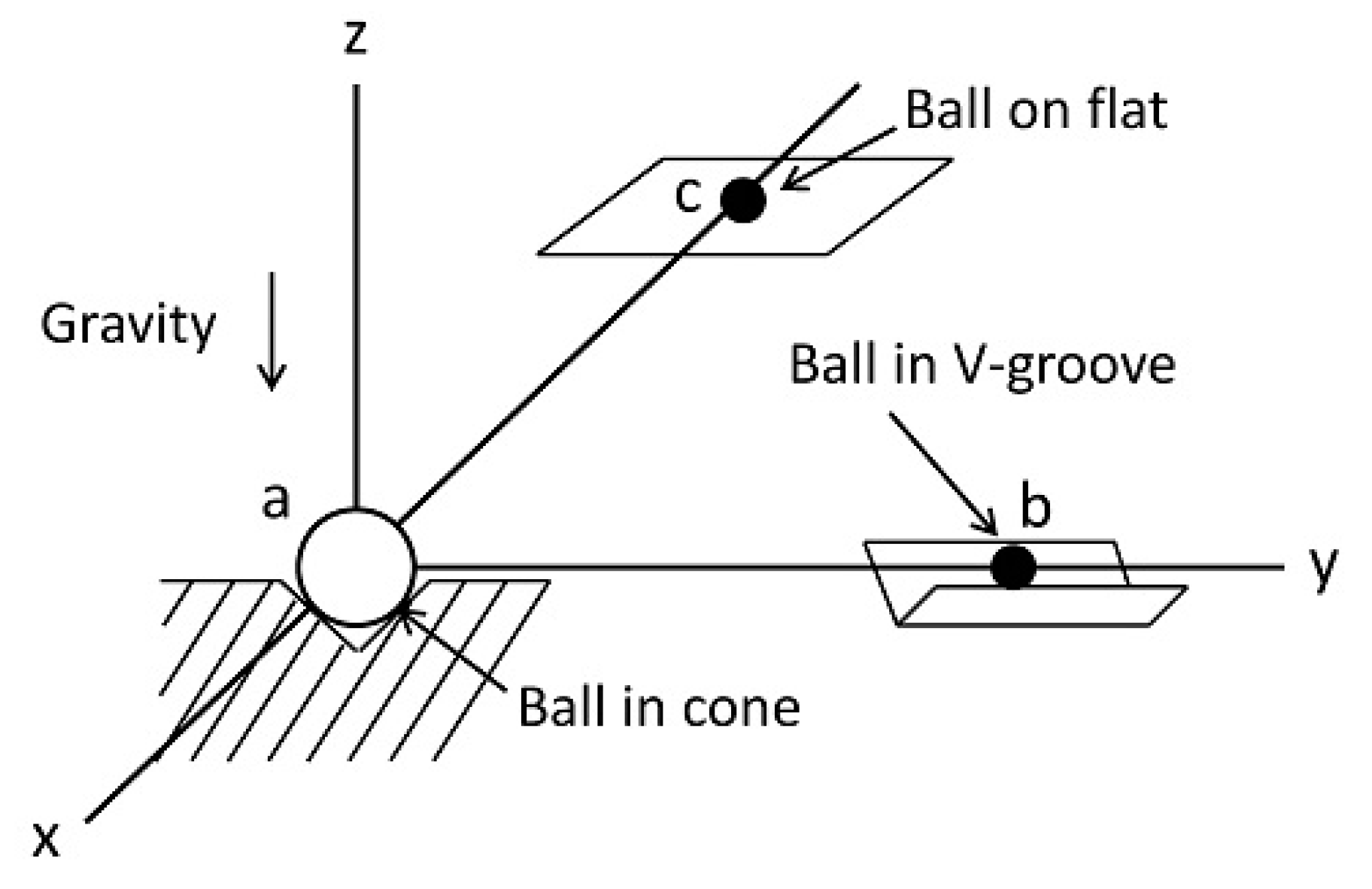
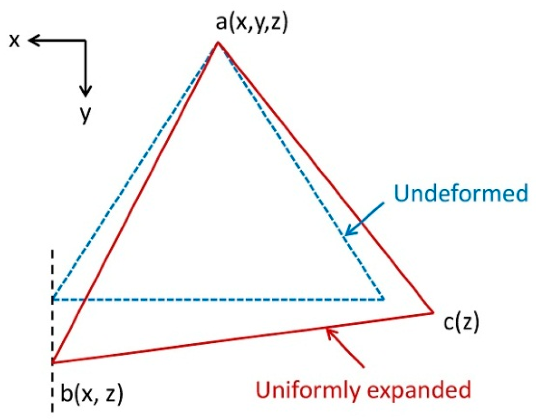
Figure 1 shows the kinematic positioning method with three positioning balls (a, b, and c). Ball a was located in the cone, which limited three translational degrees of freedom (DOF) of the rigid body and released three rotational DOF. Ball b was located in the V-groove that limited the rotational DOF around the z-axis and the line perpendicular to ab. Ball c was located on the flat that limited the rotational DOF around ab. Thus, the rigid body was limited without any over-constraint. When the temperature changed, ball b moved along the y-axis and ball c moved on the x–y plane (Figure 2). Thus, the uniform deformation of the rigid body was guaranteed without harmful thermal stress.

2.2. Mathematical Model of Rotation Angles

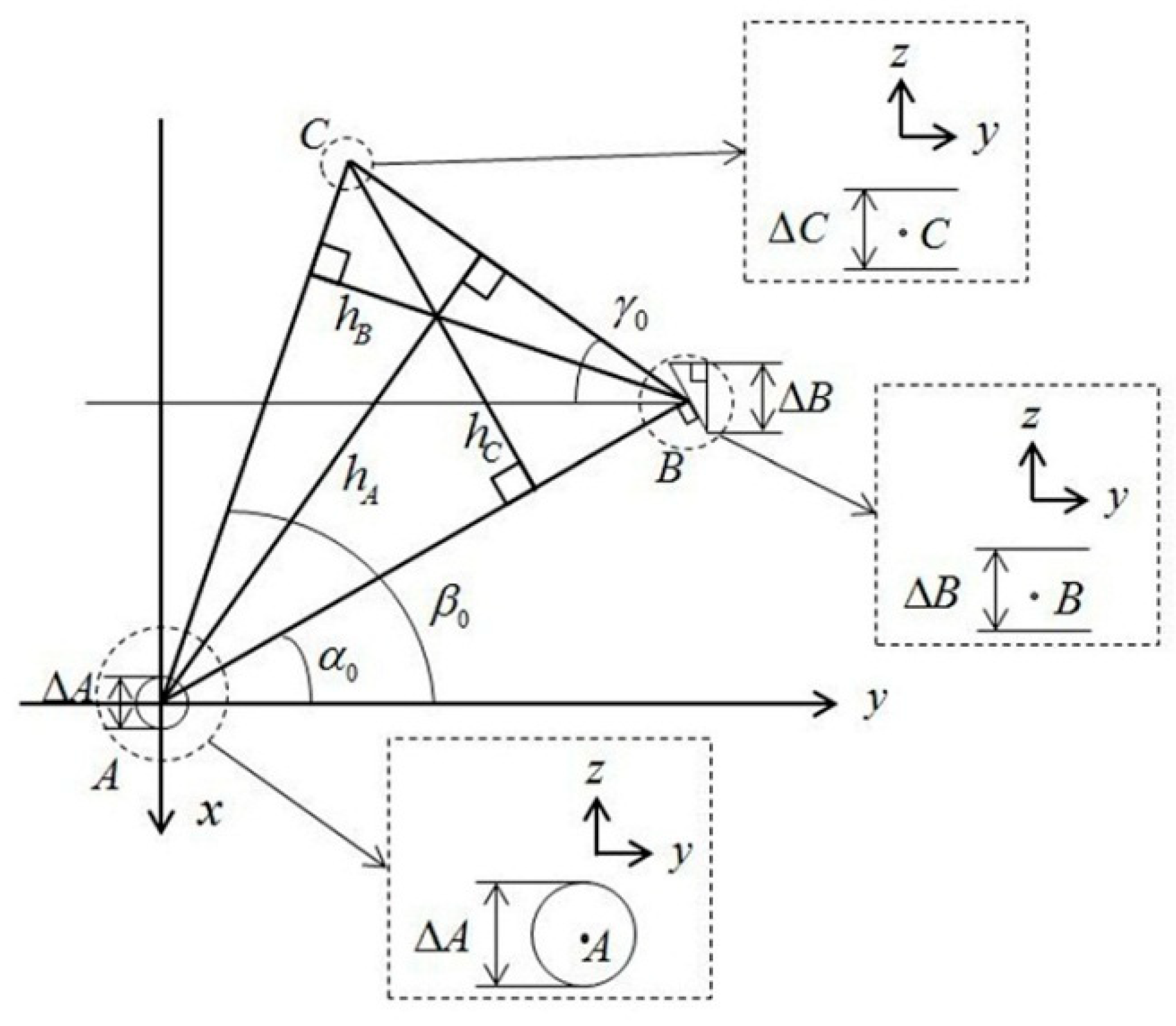
The central points of the three positioning balls were called points A, B, and C, assuming that the three points were located on the x–y plane. The infinitesimal rotation angle of a rigid body is a vector and can be calculated by using the vector operation rule [18]. The rotation of the optical unit around the x-axis and y-axis can be decomposed into rotations of the three points around the line of the other two points respectively. In addition, the rotation of the unit around the z-axis was decomposed into rotations of point A around point B and point B around point A on the x–y plane. $\Delta A$, $\Delta B$, and $\Delta C$ are the fit clearances of the positioning mechanisms consisting of the three positioning balls, respectively. The maximum rotation angles ${|{\theta }_{\mathrm{x}}|}_{\max }$, ${|{\theta }_y|}_{\max }$, and ${|{\theta }_z|}_{\max }$ of the rigid body around the x-, y-, and z-axes can be calculated by using the following equations (Figure 3):

$${|{\theta }_x|}_{\max }=|\Delta {\overrightarrow{\alpha }}_x|+|\Delta {\overrightarrow{\beta }}_x|+|\Delta {\overrightarrow{\gamma }}_x|,$$

(1)

$${|{\theta }_y|}_{\max }=|\Delta {\overrightarrow{\alpha }}_y|+|\Delta {\overrightarrow{\beta }}_y|+|\Delta {\overrightarrow{\gamma }}_y|,$$

(2)

$${|{\theta }_z|}_{\max }=|\Delta {\overrightarrow{\alpha }}_z|+|\Delta {\overrightarrow{\beta }}_z|,$$

(3)

Where $\Delta \overrightarrow{{\alpha }_x}$ and $\Delta \overrightarrow{{\alpha }_y}$ are the components of the maximum angular displacement vector of point A rotating around BC in the direction of the x-axis and y-axis, respectively. $\Delta \overrightarrow{{\beta }_x}$ and $\Delta \overrightarrow{{\beta }_y}$ are the components of the maximum angular displacement vector of point B rotating around AC in the direction of the x-axis and y-axis, respectively. $\Delta \overrightarrow{{\gamma }_x}$ and $\Delta \overrightarrow{{\gamma }_y}$ are the components of the maximum angular displacement vector of point C rotating around AB in the direction of the x-axis and y-axis, respectively. $\Delta \overrightarrow{{\alpha }_z}$ is the maximum angular displacement vector of point A rotating around point B on the x–y plane. $\Delta \overrightarrow{{\beta }_z}$ is the maximum angular displacement vector of point B rotating around point A on the x–y plane.

When a rigid body rotates around an axis by an infinitesimal angle, the direction of the angular displacement vector follows that axis. Therefore, Equations (1)–(3) can be transformed into:

$${|{\theta }_x|}_{\max }=\frac{\Delta A/2}{h_A}\sin {\gamma }_0+\frac{\Delta B/2}{h_B}\sin {\beta }_0+\frac{\Delta C/2}{h_C}\sin {\alpha }_0,$$

(4)

$${|{\theta }_y|}_{\max }=\frac{\Delta A/2}{h_A}\cos {\gamma }_0+\frac{\Delta B/2}{h_B}\cos {\beta }_0+\frac{\Delta C/2}{h_C}\cos {\alpha }_0,$$

(5)

$${|{\theta }_z|}_{\max }=\frac{\Delta A/2}{|\overrightarrow{AB}|}+\frac{\Delta B/2/\cos {\alpha }_0}{|\overrightarrow{AB}|}=\frac{1}{2}\frac{\Delta A}{|\overrightarrow{AB}|}+\frac{1}{2}\frac{\Delta B}{\overrightarrow{AB}·\overrightarrow{j}},$$

(6)

where the vector $\overrightarrow{j}=\left(0,1,0\right)$.

The angle $\phi$ between two vectors, $\overrightarrow{m}$ and $\overrightarrow{n}$, can be calculated by:

$$\sin \phi =\frac{|\overrightarrow{m}\times \overrightarrow{n}|}{|\overrightarrow{m}||\overrightarrow{n}|},$$

(7)

$$\cos \phi =\frac{\overrightarrow{m}·\overrightarrow{n}}{|\overrightarrow{m}||\overrightarrow{n}|}.$$

(8)

The height of $\Delta DFE$ can be calculated by:

$$h_D=\frac{|\overrightarrow{DE}\times \overrightarrow{EF}|}{|\overrightarrow{EF}|}.$$

(9)

Substituting Equations (7)–(9) into Equations (4) and (5) yields the following relationship:

$$\begin{array}{ll}{|{\theta }_x|}_{\max }& =\frac{\Delta A/2}{|\overrightarrow{AB}\times \overrightarrow{BC}|/\overrightarrow{|BC|}}\times \frac{|\overrightarrow{BC}\times \overrightarrow{\left(-j\right)}|}{|\overrightarrow{BC}||-\overrightarrow{j}|}+\frac{\Delta B/2}{|\overrightarrow{AB}\times \overrightarrow{AC}|/\overrightarrow{|AC|}}\times \frac{|\overrightarrow{AC}\times \overrightarrow{j}|}{|\overrightarrow{AC}||\overrightarrow{j}|}+\frac{\Delta C/2}{|\overrightarrow{AB}\times \overrightarrow{AC}|÷\overrightarrow{|AB|}}\times \frac{|\overrightarrow{AB}\times \overrightarrow{j}|}{|\overrightarrow{AB}||\overrightarrow{j}|}\\ & =\frac{1}{2}\Delta A\frac{|\overrightarrow{BC}\times \overrightarrow{j}|}{|\overrightarrow{AB}\times \overrightarrow{BC}|}+\frac{1}{2}\Delta B\frac{|\overrightarrow{AC}\times \overrightarrow{j}|}{|\overrightarrow{AB}\times \overrightarrow{AC}|}+\frac{1}{2}\Delta C\frac{|\overrightarrow{AB}\times \overrightarrow{j}|}{|\overrightarrow{AB}\times \overrightarrow{AC}|}\end{array},$$

(10)

$$\begin{array}{ll}{|{\theta }_y|}_{\max }& =\frac{\Delta A/2}{|\overrightarrow{AB}\times \overrightarrow{BC}|/\overrightarrow{|BC|}}\times \frac{\overrightarrow{BC}·\overrightarrow{\left(-j\right)}}{|\overrightarrow{BC}||-\overrightarrow{j}|}+\frac{\Delta B/2}{|\overrightarrow{AB}\times \overrightarrow{AC}|/\overrightarrow{|AC|}}\times \frac{\overrightarrow{AC}·\overrightarrow{j}}{|\overrightarrow{AC}||\overrightarrow{j}|}+\frac{\Delta C/2}{|\overrightarrow{AB}\times \overrightarrow{AC}|/\overrightarrow{|AB|}}\times \frac{\overrightarrow{AB}·\overrightarrow{j}}{|\overrightarrow{AB}||\overrightarrow{j}|}\\ & =\frac{1}{2}\Delta A\frac{\overrightarrow{CB}·\overrightarrow{j}}{|\overrightarrow{AB}\times \overrightarrow{BC}|}+\frac{1}{2}\Delta B\frac{\overrightarrow{AC}·\overrightarrow{j}}{|\overrightarrow{AB}\times \overrightarrow{AC}|}+\frac{1}{2}\Delta C\frac{\overrightarrow{AB}·\overrightarrow{j}}{|\overrightarrow{AB}\times \overrightarrow{AC}|}\end{array}.$$

(11)

2.3. Design of Fit Clearance

By substituting the relative position relationships of the positioning points into Equation (6) and Equations (10) and (11), the simplified expressions of these equations can be obtained. In addition, because the index requirements of the re-orientation angles around three axes were not more than 12″, the above equations can be expressed by the following matrix:

$$\left[\begin{array}{ccc}\frac{234}{1541052}& \frac{885}{1541052}& \frac{651}{1541052}\\ \frac{822}{1541052}& \frac{184}{1541052}& \frac{1006}{1541052}\\ \frac{1}{2396.6}& \frac{1}{2012}& 0\end{array}\right]\left[\begin{array}{c}\Delta A\\ \Delta B\\ \Delta C\end{array}\right]=\left[\begin{array}{c}\frac{\pi }{54000}\\ \frac{\pi }{54000}\\ \frac{\pi }{54000}\end{array}\right].$$

(12)

When the maximum rotation angles around three axes were all 12″, the fit clearances that were obtained from Equation (12) were $\Delta A=0.062$ mm, $\Delta B=0.065$ mm, $\Delta C=0.027$ mm. Within this range, considering the operating and manufacturing factors, the design values were calculated as $\Delta A=0.02$ mm, $\Delta B=0.06$ mm, and $\Delta C=0.02$ mm. By substituting $\Delta A$, $\Delta B$, and $\Delta C$ into Equation (6) and Equations (10) and (11), we obtained ${|{\theta }_x|}_{\max }=$ 9.5″, ${|{\theta }_y|}_{\max }=$ 6.4″, and ${|{\theta }_z|}_{\max }=$ 7.9″.

3. Rotation Angle Measurement Principle and Error Analysis

3.1. Rotation Angle Measurement Principle

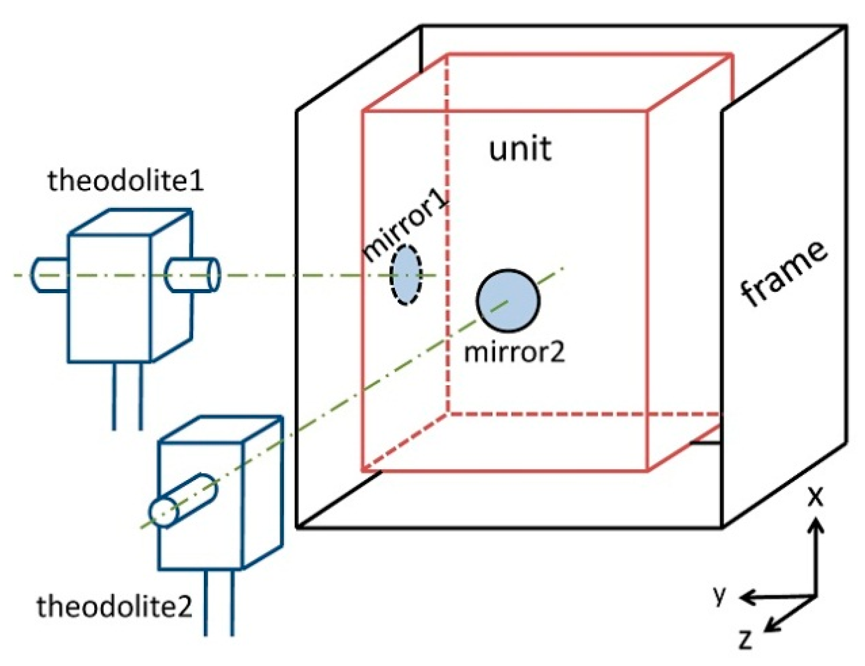
Two theodolites and two plane mirrors were used to measure the rotation angles of the optical unit (Figure 4). The rotation angles around the x- and z-axes of the unit were obtained from the azimuth and pitch angles of theodolite1, respectively. At the same time, the rotation angles around the x- and y-axes of the unit were obtained from the azimuth and pitch angles of theodolite2, respectively. The rotation angle around the x-axis was measured by the two theodolites at the same time, so that the two theodolites could calibrate each other. In order to obtain the re-orientation accuracy, the unit was inserted into and extracted from the frame several times, and the re-orientation accuracy was found by recording the azimuth and pitch angles of theodolites.

3.2. Measurement Error Analysis

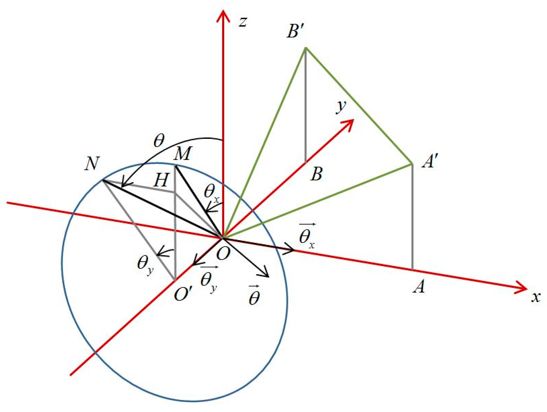
The initial position of the mirror is represented by the plane OAB on the x–y plane, as shown in Figure 5. After rotating around the x-axis by infinitesimal angle ${\theta }_x$ and then rotating around the y-axis by infinitesimal angle $-{\theta }_y$, the mirror moved onto the plane $O{A}^{\prime }{B}^{\prime }$. The angular displacement vectors were $\overrightarrow{{\theta }_x}=\left({\theta }_x,0,0\right)$ and $\overrightarrow{{\theta }_y}=\left(0,-{\theta }_y,0\right)$. The normal vector of the mirror changed from the z-axis to $\overrightarrow{OM}$ and then to $\overrightarrow{ON}$. It was also observed that plane OAB rotated to plane $O{A}^{\prime }{B}^{\prime }$ by one step with a rotation angle $\theta$ and an angular displacement vector $\overrightarrow{\theta }$. $NH$ was perpendicular to the y–z plane at point $H$, assuming that the angle between $OH$ and the z-axis was ${\theta }_{cx}$, as well as $\angle HON={\theta }_{cy}$. The positions of the theodolites indicated that ${\theta }_{cx}$ was the same as the difference between the azimuth angles of theodolite2 before and after rotating, while $-{\theta }_{cy}$ was the same as the difference between the pitch angles of theodolite2 before and after rotating. The rotation around the z-axis slightly affected the rotation angles around the x- and y-axes if the z-axis rotation angle was infinitesimal. Thus, we ignored the z-axis rotation.

Let $|\overrightarrow{OM}|=|\overrightarrow{ON}|=1$. Thus,

$$\overrightarrow{ON}=\left(-\cos {\theta }_x\sin {\theta }_y,-\sin {\theta }_x,\cos {\theta }_x\cos {\theta }_y\right)$$

(13)

$$\overrightarrow{OH}=\left(0,-\sin {\theta }_x,\cos {\theta }_x\cos {\theta }_y\right).$$

(14)

${\theta }_{cx}$ and ${\theta }_{cy}$ were calculated using the following equations:

$${\theta }_{cx}=\arccos \frac{\overrightarrow{k}·\overrightarrow{OH}}{|\overrightarrow{k}||\overrightarrow{OH}|}=\arccos \frac{\cos {\theta }_x\cos {\theta }_y}{\sqrt{{\cos }^2{\theta }_x{\cos }^2{\theta }_y+{\sin }^2{\theta }_x}},$$

(15)

$${\theta }_{cy}=\arccos \frac{\overrightarrow{ON}·\overrightarrow{OH}}{|\overrightarrow{ON}||\overrightarrow{OH}|}=\arccos \sqrt{{\cos }^2{\theta }_x{\cos }^2{\theta }_y+{\sin }^2{\theta }_x},$$

(16)

where $\overrightarrow{k}=\left(0,0,1\right)$.

${\theta }_x$ and ${\theta }_y$ were expressed using the following equations in terms of Equations (15) and (16):

$${\theta }_x=\arcsin \left(\sin {\theta }_{cx}\cos {\theta }_{cy}\right),$$

(17)

$${\theta }_y=\arccos \frac{\cos {\theta }_{cx}\cos {\theta }_{cy}}{\sqrt{1-{\sin }^2{\theta }_{cx}{\cos }^2{\theta }_{cy}}}.$$

(18)

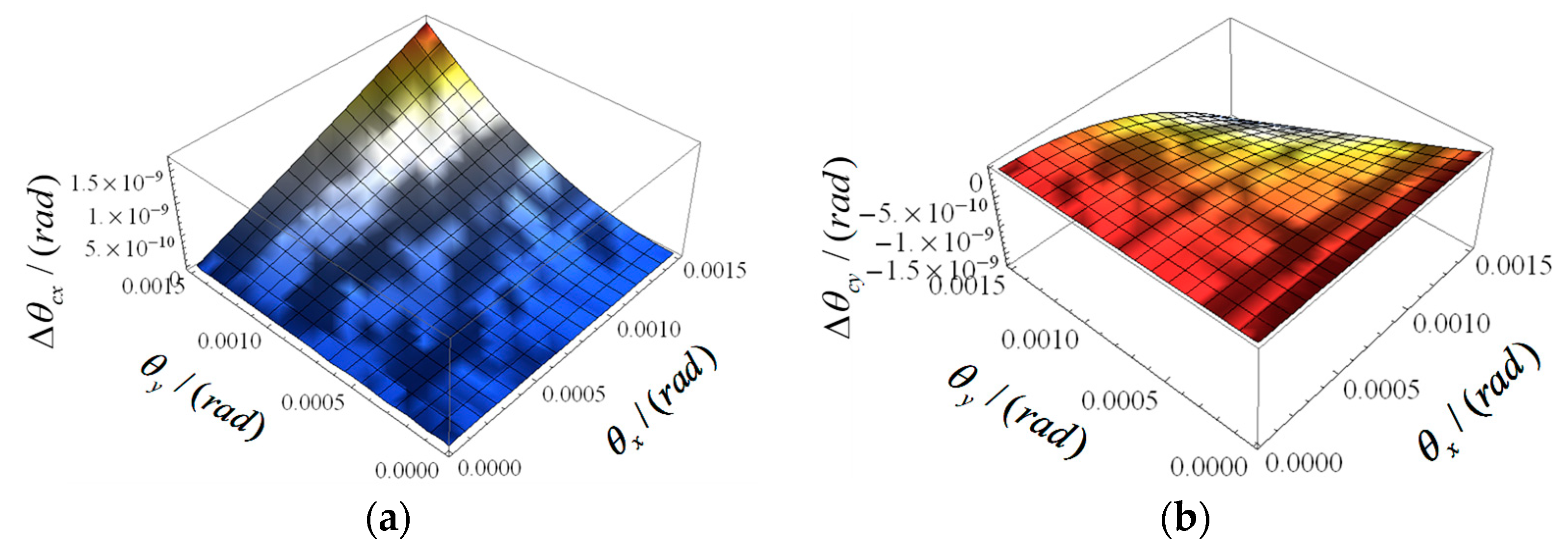
To derive the differences between $|\Delta {\theta }_{cx}|$, $|\Delta {\theta }_{cy}|$ and $|\overrightarrow{{\theta }_x}|$, $|\overrightarrow{{\theta }_y}|$ under some limits, some numerical simulations were carried out by using Mathematica. Assuming that $\Delta {\theta }_{cx}=|{\theta }_{cx}|-|\overrightarrow{{\theta }_x}|$ and $\Delta {\theta }_{cy}=|{\theta }_{cy}|-|\overrightarrow{{\theta }_y}|$, the relationship between the differences and ${\theta }_x$, ${\theta }_y$ is shown in Figure 6. Thus, some simple unit transformations were used to draw the conclusion that $|\Delta {\theta }_{cx}|$ and $|\Delta {\theta }_{cy}|$ were both no more than ${0.0003}^{″}$ when $|\overrightarrow{{\theta }_x}|$ and $|\overrightarrow{{\theta }_y}|$ were not more than ${300}^{″}$. In other words, if the two real angles were both not more than ${300}^{″}$, the difference between the azimuth angles of theodolite2 before and after rotating was nearly equal to the real rotation angle of the unit around the x-axis, and the difference between the pitch angles of theodolite2 before and after rotating was nearly equal to the real rotation angle of the unit around the y-axis. For the same reason, when the real angles around the x-and z-axes were both not more than ${300}^{″}$, the difference between the azimuth angles of theodolite1 before and after rotating was nearly equal to the real rotation angle of the unit around the x-axis, and the difference between the pitch angles of theodolite1 before and after rotating was nearly equal to the real rotation angle of the unit around the z-axis.

4. Experiment and Discussion

4.1. Experimental Settings

Existing microgravity simulation methods are mainly classified into five categories, namely, parabolic flight, drop tower, suspension method, neutral buoyancy, and air-bearing suspension methods [8,19]. Compared with the other methods, the suspension method has the advantages of low cost, relatively simple structure, unlimited simulation time, freedom from the influence of liquid resistance and fluidity on the simulation accuracy, and realization of 3-dimensional motion simulation [20,21,22]. Therefore, the suspension method was used to simulate the space microgravity environment in this experiment.

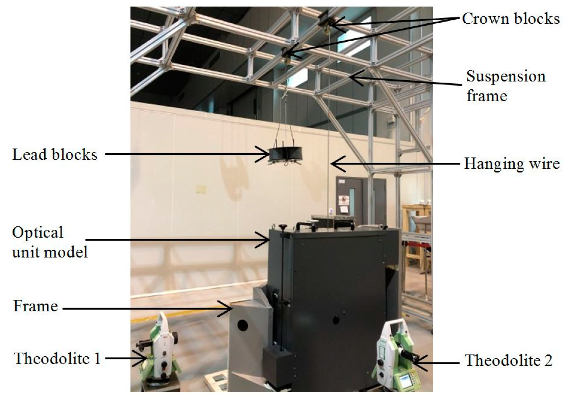
An experiment was designed to verify the correctness of the mathematical models of the relationship between fit clearances and rotation angles. We simulated the optical unit and frame with square steel tubes, and the optical unit was fixed on the frame by positioning mechanisms. Two crown blocks were fixed on the suspension frame, and a hanging wire was passed through the crown blocks. One end of the hanging wire lifted some lead blocks that were the same weight as the optical unit model in total, and the other end was fixed at the center-of-mass position of the optical unit model. Two perpendicular plane mirrors were fixed on the optical unit model. One was parallel to the z–x plane and the other was parallel to the x–y plane. Two theodolites (Leica TM6100A-from Leica Geosystems AG, Heerbrugg, Switzerland: resolution is 0.1″ when angle display mode is 360°′″, and accuracy is 0.5″) were placed on the central axis of the two mirrors respectively. Figure 7 shows the experimental system.

4.2. Experimental Results and Discussion

The optical unit model was removed from the frame and then inserted back into it. After insertion, it was fixed on the frame by positioning mechanisms. At that time, the corresponding azimuth and pitch angles of the theodolites were recorded (as

Table 1. Experiment results.

	Azimuth Angle of Theodolite1 (Relating to the Rotation Angle Around the x-Axis of the Model)	Azimuth Angle of Theodolite2 (Relating to the Rotation Angle Around the x-Axis of the Model)	Pitch Angle of Theodolite2 (Relating to the Rotation Angle Around the y-Axis of the Model)	Pitch Angle of Theodolite1 (Relating to the Rotation Angle Around the z-Axis of the Model)
	Test Results (″)	Test Results (″)	Test Results (″)	Test Results (″)
1	−22.3	−51.2	12.8	3.3
2	−24.2	−56.2	13.1	7.7
3	−26.4	−54.4	11.6	8.4
4	−18.4	−52.8	13.0	8.5
5	−20.9	−49.5	13.3	4.3
6	−21.2	−52.2	9.0	4.4
7	−22.3	−54.0	10.1	12.5
8	−24.8	−56.5	7.2	3.8
9	−22.0	−52.3	11.0	8.9
10	−21.7	−52.1	10.4	8.7
Re-orientation error ($3\sigma$-confidence interval)	6.4	6.2	5.7	8.5

). The above steps were repeated 10 times.

In addition to the measurement results, the re-orientation errors expressed by the $3\sigma$-confidence interval (calculated by the following equation [23]) are also listed in Table 1.

$$\Delta \left(x\right)=3\sigma ,$$

(19)

where $\sigma$ is the standard deviation of a group of measurement results.

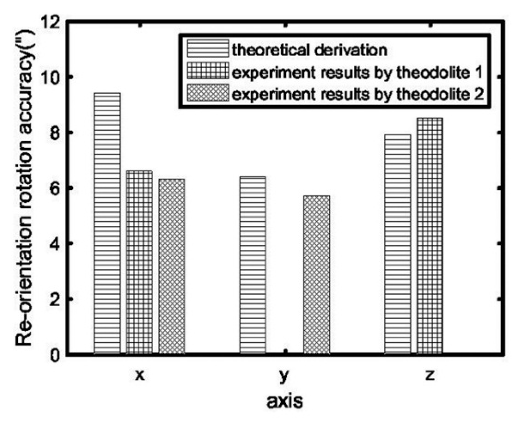
As shown in Figure 8, the re-orientation errors in the experiment basically accorded with the theoretical derivation. However, there were some acceptable errors between the experimental results and theoretical derivation due to errors in machining, installation, instruments, and personnel, etc. Besides, because the hoisting point of the optical unit model did not completely coincide with the center of mass and there were errors in the gravity unloading device which sometimes led to gravity unloading instability, the standard deviation $\sigma$ of the measurement results around the z-axis got larger. As a result, the re-orientation error around the z-axis was higher than the theoretical limit.

5. Conclusions

In this paper, the re-orientation accuracy of an on-orbit replaceable optical unit was studied. Based on the angular displacement vector, the mathematical models of the relationship between fit clearances and theoretical rotation angle limits were deduced. When the relative position relationship of the positioning mechanisms was known, the fit clearances of positioning mechanisms as the key factor of re-orientation accuracy were designed using a matrix. This was a simple method to design the fit clearances. The rotation angle measurement method by the theodolites was introduced and error analysis was carried out. The analysis results showed that the differences between the measurement angles and the real angles were within limits. The experiment was designed and the gravity of the optical unit model was unloaded. The experimental results showed that the rotation accuracy around the x-axes of the optical unit was 6.4″ (by theodolite1) and 6.2″ (by theodolite2), the accuracy around the y-axes was 5.7″, and the accuracy around the z-axes was 8.5″. The results were within the index range, and there were some acceptable errors, which accorded with the theoretical deduction. The correctness of designing the fit clearances by mathematical models was proved. This study provides a reference for the design of the fit clearances of on-orbit replaceable units.

References

- Coleshill, E.; Oshinowo, L.; Rembala, R.; Bina, B.; Rey, D.; Sindelar, S. Dextre: Improving maintenance operations on the International Space Station. Acta Astronaut. 2009, 64, 869–874. [Google Scholar] [CrossRef]
- Joppin, C.; Hastings, D.E. On-orbit upgrade and repair: The Hubble Space Telescope example. J. Spacecr. Rocket. 2006, 43, 614–625. [Google Scholar]
- Leete, S.J. Design for on-orbit spacecraft servicing. In Proceedings of the 2001 Core Technologies for Space Conference, Colorado Springs, CO, USA, 28–30 November 2001. [Google Scholar]
- Shayler, D.J.; Harland, D.M. The Hubble Space Telescope: From Concept to Success; Springer: Berlin, Germany, 2015. [Google Scholar]
- Akin, D.; Roberts, B.; Pilotte, K.; Baker, M. Robotic augmentation of EVA for Hubble Space Telescope servicing. In Proceedings of the AIAA Space 2003 Conference & Exposition, Long Beach, CA, USA, 23–25 September 2003. [Google Scholar]
- King, D. Hubble robotic servicing: Stepping stone for future exploration missions. In Proceedings of the 1st Space Exploration Conference: Continuing the Voyage of Discovery, Orlando, FL, USA, 30 January–1 February 2005. [Google Scholar]
- Ji, Y.X. Conceptual Study of Spacecraft Replacement Unit for On-Orbit Servicing. Master’s Thesis, Nanjing University of Aeronautics and Astronautics, Nanjing, China, 2016. [Google Scholar]
- Flores-Abad, A.; Ma, O.; Pham, K.; Ulrich, S. A review of space robotics technologies for on-orbit servicing. Prog. Aerosp. Sci. 2014, 68, 1–26. [Google Scholar] [CrossRef] [Green Version]
- Chen, X.; Yuan, J.; Yao, W. The Technology of On-Orbit Spacecraft Servicing; China Astronautic Publishing House: Beijing, China, 2009; pp. 1–22. [Google Scholar]
- Huang, B.; Liu, T.; Han, J.; Hu, H. Polarimetric target detection under uneven illumination. Opt. Express 2015, 23, 23603–23612. [Google Scholar] [CrossRef] [PubMed]
- Liu, M.; Zhang, X.; Liu, T.; Shi, G.; Wang, L.; Li, Y. On-orbit polarization calibration for multichannel polarimetric camera. Appl. Sci. 2019, 9, 1424. [Google Scholar] [CrossRef]
- Liu, X.; Wang, F.; Zhang, M.; Cai, Y. Effects of atmospheric turbulence on lensless Ghost Imaging with partially coherent light. Appl. Sci. 2018, 8, 1479. [Google Scholar] [CrossRef]
- Zhu, J.; Sha, W.; Chen, C.; Zhang, X.; Ren, J. Frequency response of imaging quality by micro-vibration for large-aperture space-borne telescope. Opt. Precis. Eng. 2016, 24, 1118–1127. [Google Scholar]
- Yu, L.; Chen, J.; Xue, H.; Shen, Y. Hyper-spectral imaging sensor in UV-VIS-NIR region in air for costal ocean observation. Opt. Precis. Eng. 2018, 26, 2363–2370. [Google Scholar]
- Cao, H.; Li, B.; Li, Y.; Kang, T.; Chen, X. Model-based error motion prediction and fit clearance optimization for machine tool spindles. Mech. Syst. Signal Process. 2019, 133, 106252. [Google Scholar] [CrossRef]
- Leonov, O.A.; Shkaruba, N.Z. A parametric failure model for the calculation of the fit tolerance of joints with clearance. J. Frict. Wear 2019, 40, 332–336. [Google Scholar] [CrossRef]
- Wang, J.; Ning, K.; Tang, L.; Malekian, R.; Liang, Y.; Li, Z. Modeling and finite element analysis of load-carrying performance of a wind turbine considering the influence of assembly factors. Appl. Sci. 2017, 7, 298. [Google Scholar] [CrossRef]
- From, P.J.; Gravdahl, J.T.; Pettersen, K.Y. Rigid Body Dynamics; Springer: Berlin, Germany, 2014; pp. 132–133. [Google Scholar]
- Xiang, S. Dynamic Modeling and Contorl Analysis for Suspended Type Astronauts Low-Gravity Simulation System. Master’s Thesis, Harbin Institute of Technology, Harbin, China, 2015. [Google Scholar]
- Nicolau, E.; Poventud-Estrada, C.M.; Arroyo, L.; Fonseca, J.; Flynn, M.; Cabrera, C.R. Microgravity effects on the electrochemical oxidation of ammonia: A parabolic flight experiment. Electrochim. Acta 2012, 75, 88–93. [Google Scholar] [CrossRef]
- Belser, V.; Breuninger, J.; Reilly, M.; Laufer, R.; Dropmann, M.; Herdrich, G.; Hyde, T.; Röser, H.-P.; Fasoulas, S. Aerodynamic and engineering design of a 1.5 s high quality microgravity drop tower facility. Acta Astronaut. 2016, 129, 335–344. [Google Scholar] [CrossRef]
- Newman, D.J.; Alexander, H.L. Human locomotion and workload for simulated lunar and Martian environments. Acta Astronaut. 1993, 29, 613–620. [Google Scholar] [CrossRef]
- Ma, H.; Wang, J. Instrument Accuracy Theory; Beihang University Press: Beijing, China, 2014; pp. 50–51. [Google Scholar]
Figure 1.
Kinematic positioning method. The three positioning balls are on the x–y plane.
Figure 2.
Movement trend of the rigid body when the temperature changes. The dotted triangle represents the initial position of the rigid body, and the solid triangle represents the rigid body after the temperature changes. The letters in brackets correspond to the directions of the translational degrees of freedom (DOF) restricted by each ball.
Figure 3.
Layout of points A, B, and C and their fit clearances , , and . , , and are the heights of .
Figure 4.
Measurement principle and coordinate systems. Two mirrors were fixed on the unit and were perpendicular to each other. The y-axis and the z-axis were parallel to the central lines of the two mirrors, respectively. In addition, two theodolites were placed on the center lines of the two mirrors, respectively.
Figure 5.
Schematic of mirror rotation. is the normal vector of the mirror plane that rotates infinitesimal angle around the x-axis; is the normal vector of the mirror plane that rotates infinitesimal angle around the y-axis. The circle passing through points M and N is parallel to the z–x plane.
Figure 6.
Relationship between the infinitesimal angle , and the differences when rad and rad: (a) The difference is ; (b) The difference is .
Figure 7.
Photograph of the experimental system.
Figure 8.
Re-orientation accuracy results of the theoretical derivation and experiment. The re-orientation accuracies in the experiment around the x- and y-axes were slightly less than the theoretical derivation, whereas the accuracy around the z-axis was slightly greater than the theoretical derivation.