Sample Reduction Strategies for Protein Secondary Structure Prediction

Abstract

Predicting the secondary structure from protein sequence plays a crucial role in estimating the 3D structure, which has applications in drug design and in understanding the function of proteins. As new genes and proteins are discovered, the large size of the protein databases and datasets that can be used for training prediction models grows considerably. A two-stage hybrid classifier, which employs dynamic Bayesian networks and a support vector machine (SVM) has been shown to provide state-of-the-art prediction accuracy for protein secondary structure prediction. However, SVM is not efficient for large datasets due to the quadratic optimization involved in model training. In this paper, two techniques are implemented on CB513 benchmark for reducing the number of samples in the train set of the SVM. The first method randomly selects a fraction of data samples from the train set using a stratified selection strategy. This approach can remove approximately 50% of the data samples from the train set and reduce the model training time by 73.38% on average without decreasing the prediction accuracy significantly. The second method clusters the data samples by a hierarchical clustering algorithm and replaces the train set samples with nearest neighbors of the cluster centers in order to improve the training time. To cluster the feature vectors, the hierarchical clustering method is implemented, for which the number of clusters and the number of nearest neighbors are optimized as hyper-parameters by computing the prediction accuracy on validation sets. It is found that clustering can reduce the size of the train set by 26% without reducing the prediction accuracy. Among the clustering techniques Ward’s method provided the best accuracy on test data.

1. Introduction

The four different levels of protein structure are known as primary, secondary, tertiary and quaternary structure. The primary structure consists of amino acids that are linked by peptide bonds that make up the protein. The secondary structure is the local conformation of amino acids through hydrogen bonding interactions into regular structures. The three common types of secondary structures are the $\alpha$-helices, $\beta$-sheets and coils (or loops). Secondary structure elements and motifs come together to form tertiary structure. The tertiary structure is the global three-dimensional structure of an amino acid chain or a domain within a protein. Finally quaternary structure refers to multiple chains uniting together via chemical bonds that operate as a single functional unit [1,2].

There are millions of amino acid sequences in protein databases and it is essential to annotate them according to their structural and functional roles [3]. For instance, predicting the one-dimensional properties of proteins such as secondary structure and solvent accessibility plays a crucial role in predicting the 3D structure and understanding the function of proteins [4,5]. Several classification methods have been proposed in the literature for this purpose such as neural networks [6,7], support vector machines [8], dynamic Bayesian networks [9] and hybrid methods that combine different classifiers [9,10]. To date, most of the research efforts in this field have concentrated on developing advanced prediction methods. In the mean time, as new genes and proteins are discovered, the size of the protein databases and datasets that can be used for training prediction models grows considerably. Therefore efficient algorithms and/or data reduction strategies should be developed that can circumvent the computational cost caused by big data conditions while incorporating the useful information into prediction models. Though there are methods developed for reducing the number of features (i.e., dimensions) of the classifiers by employing feature selection or dimension reduction techniques [11], to the best of our knowledge, there is no work in the literature for reducing the number of train set samples using techniques such as sampling and clustering for predicting one-dimensional structural properties of proteins. Recently, a new database called UniClust has been introduced that is derived by clustering millions of proteins [12]. This database is introduced as the sequence database of the HHblits method [13], which aligns a query protein against the amino acid sequences in the database. There are also other databases introduced earlier such as SCOP [14] and PFAM [15] that organize proteins hierarchically into multiple levels (e.g., family, superfamily, fold, class, domain or clan). Among those SCOP assigns proteins to families based on multiple criteria and using clustering. However none of these databases and clustering approaches are employed directly to reduce the size of the train set of a machine learning classifier for predicting structural properties of proteins.

In this paper, the DSPRED method is employed to predict the secondary structure of proteins, which is a two-stage hybrid classifier that combines dynamic Bayesian networks and a support vector machine (SVM). SVMs are known to be effective for combining heterogenous input features as in DSPRED which employs PSSM features as well as features in the form of probability distributions (see Section 3.4). It has been shown in Aydin et al. that replacing SVM with other standard classifiers did not improve the accuracy of DSPRED [16]. One drawback of the SVM is high computational complexity in model training, which can be prohibitive for large datasets [17]. To address this problem, different approaches have been proposed in the literature such as stratified sampling [18], random selection [19], clustering analysis [19], de-clustering [20] and Learning Vector Quantization (LVQ) neural network [21]. In the present study, random stratified sampling and clustering techniques are employed in order to reduce the number of data samples used for training the SVM classifier of the DSPRED method. Note that no matter which classifier is used, reducing the dataset size by reducing the number of data samples will improve the speed of making predictions, which is useful considering the fact that the protein data in public databases is growing rapidly. As an alternative to sample reduction, dimension reduction techniques such as feature selection can also be employed to reduce the training time of the SVM. This is explored in Aydin et al. [11] and Xie et al. [22] and deserves a separate analysis. It should be noted that in Aydin et al. [11] reducing the dimensions by feature selection did not improve the accuracy of prediction. Therefore in this work, we reduce the number of samples not only to reduce the model training time of the SVM but also to explore whether the prediction accuracy will improve.

2. Related Studies

In this section, we give a brief review of the literature that employs SVMs for secondary structure prediction and studies that propose methods for reducing the training time of the SVM through sample reduction. Lin et al. proposed a multi-SVM ensemble to improve the performance of secondary structure prediction. Their method contains two layers: the first layer consists of an ensemble of five classifiers and the second layer is built by three SVMs. The multi-SVM ensemble employs bagging to resample the training dataset through bootstrap sampling and achieves improved performance on secondary structure prediction when a seven fold cross-validation is performed on the RS126 dataset [23]. Hua et al. proposed a new method of protein secondary structure prediction which is based on the support vector machine (SVM). Their method achieves a three-state per-residue accuracy (Q3) of 73.5% by seven fold cross validation on the CB513 dataset [24]. Although there are many other publications that employ SVMs for protein secondary structure prediction, none of these include sample reduction for reducing the training time of the SVM. Therefore we continue with methods that improve the model training time of SVM in other problems. Jun employed stratified sampling to select a subset of examples from training set [18]. In this work, the author selected 10% of the samples from each class, which reduces the size of the training set by 10-fold. Then an SVM classifier is trained using the reduced dataset. The method is applied to four datasets from UCI Machine Learning repository. Though the prediction accuracy of the models trained by 10% stratified sampling is maintained for the adult and iris datasets, it reduced considerably as compared to using all the samples for letter image recognition and protein location sites datasets. In another work, Hens and Tiwari reduced the number of features by F-score and stratified sampling for credit scoring problem and obtained similar accuracy as the other state-of-the-art methods while reducing the computational time significantly [25]. In addition to sampling strategies, there are also methods that employ clustering to reduce the sample size of the training sets. Awad et al. [19] employed a hierarchical clustering approach to improve the training time of an SVM particularly for large datasets. They proposed three techniques named TCT-SVM, TCTD-SVM and OTC-SVM, which are shown to work efficiently for model training. Among those TCT-SVM performed better than the others in terms of accuracy but it had a higher model training time [19]. Yu et al. have proposed a new method called CB-SVM (Clustering-Based SVM) that integrates a scalable clustering method for large datasets while generating high classification accuracy. The authors claim that the CB-SVM algorithm can reduce the total number of data points effectively for training an SVM [20].

3. Materials and Methods

3.1. Dataset

To further validate our method, we applied it to the non-homologous CB513 dataset constructed by Reference [26], which contains 513 protein chains and 84,119 amino acids. This dataset is one of the standard benchmarks in protein secondary structure prediction to assess the accuracy of algorithms [27]. It contains protein sequences and structure label assignments obtained using the DSSP program [28] starting from the structure information in Protein Data Bank (PDB) [29]. The DSSP convention is used to map 8-state representation of secondary structure labels into 3-state by applying the following conversion rule: H, G, I to H; E, B to E; S, T, to L.

3.2. Problem Definition

Starting from an amino acid sequence, in secondary structure prediction problem, the goal is to assign a structural class label from a 3-letter alphabet (H: Helix, E: Strand, L: Loop) to each amino acid of the protein (Figure 1).

3.3. Feature Extraction for Protein Secondary Structure Prediction

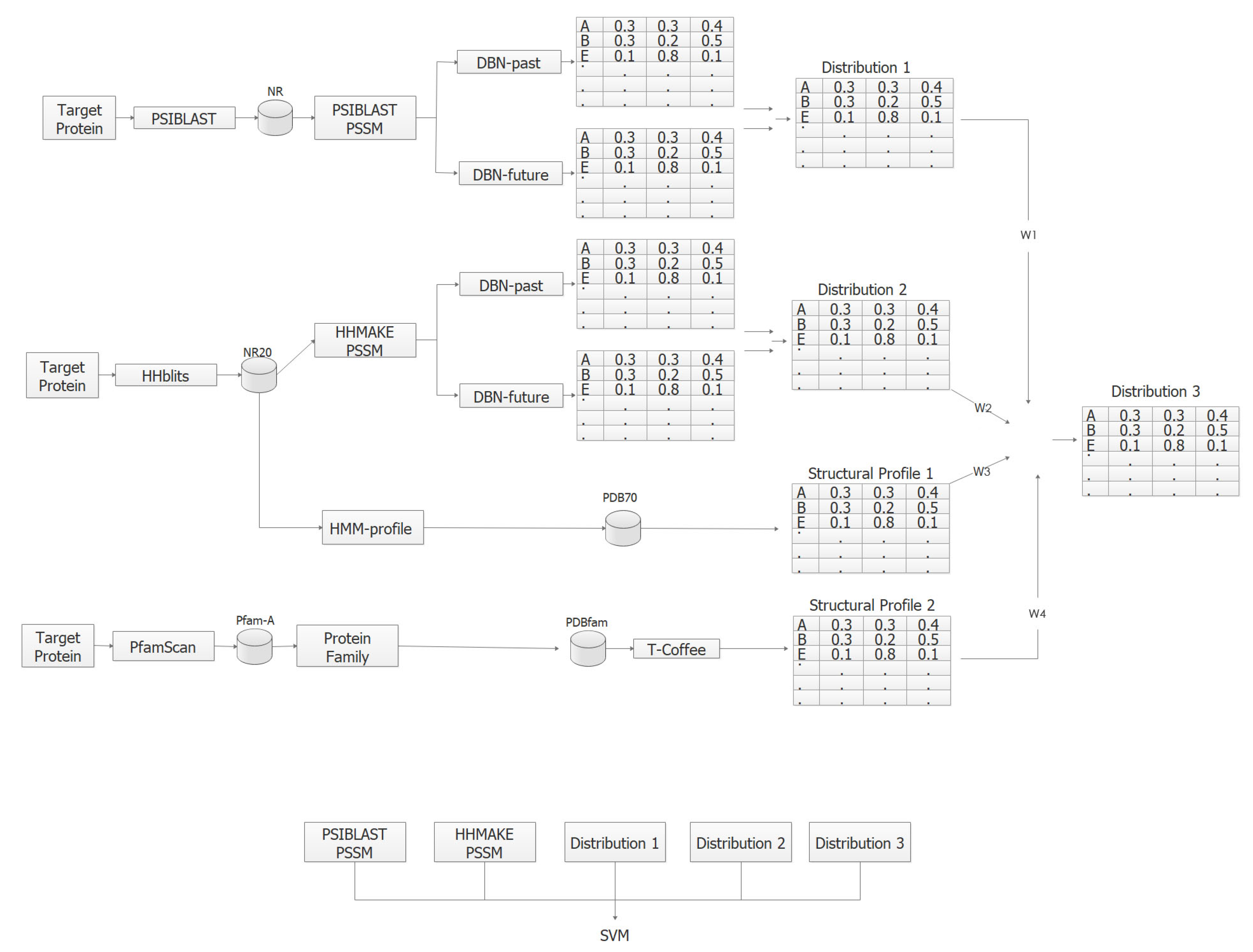
The input features of our prediction methods include sequence profiles in the form of position-specific scoring matrices (PSSMs) [30] derived by PSI-BLAST [31], HHMAKE PSSMs as well as structural profile matrices. Each target protein in the CB513 benchmark is aligned with the proteins of the NCBI’s NR database [32] using the PSI-BLAST method [31] to compute a position specific scoring matrix (PSSM). In the next step, the proteins that are similar to target are aligned jointly by a multiple alignment algorithm and a PSSM is computed by normalizing the frequency of occurrence counts of amino acids [31]. Similarly, HHMAKE PSSMs are computed by aligning the target proteins against the NR20 database (a reduced version of the NR) using the HHblits (https://toolkit.tuebingen.mpg.de/tools/hhblits) method and converting the HMM-profile model’s match state distributions to a frequency table. In the next step, the HMM-profile of the target is aligned against the HMM-profiles in the PDB70 [33] database using the second step of the HHblits method. To generate structural profiles, the HMM-profile of the target is aligned against the HMM-profiles in the PDB70 [33] database using the second step of the HHblits method.

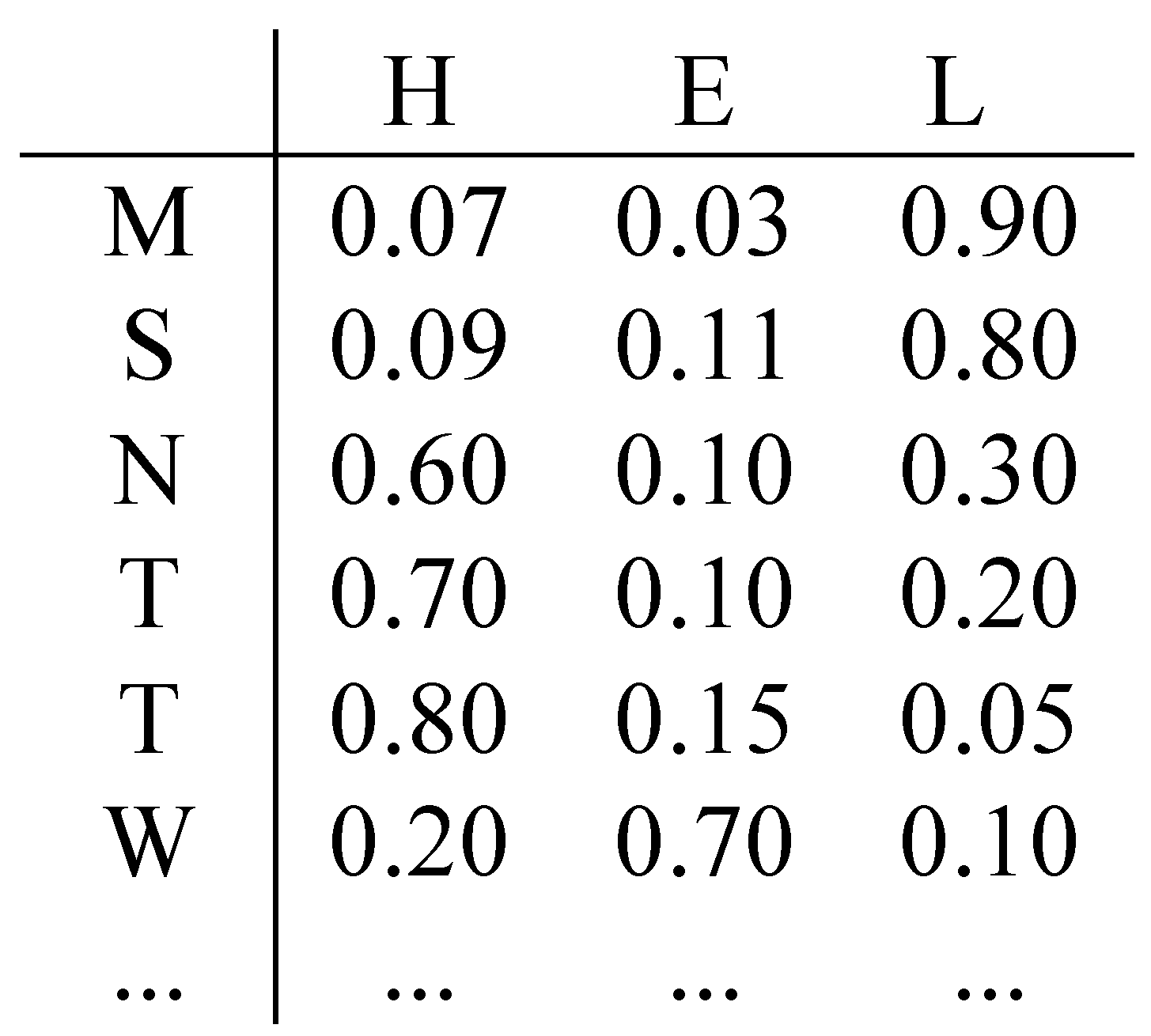
The size of the PSI-BLAST and HHMAKE PSSMs are N by 20 and the size of the structural profile matrix is N by 3, where N is the number of amino acids in the target protein. Each row of PSI-BLAST and HHMAKE PSSM contains the propensity of observing one of the 20 amino acids at a particular amino acid of the target. On the other hand, each row of structural profile matrix and the three distributions in Section 3.4 contains the probability of observing the three secondary structure labels at a particular amino acid of the target. An example structural profile matrix is shown in Figure 2. In the present study, only distant templates are used to construct structural profiles matrices by removing templates for which the percentage of sequence identity score with respect to target is greater than 20%. Once the profile matrices are obtained they are scaled by sigmoidal transformation to transform the features to the range [0, 1], which are sent as input to DSPRED method for classification. Details of feature extraction can be found in Aydin et al. [9] and the thesis work of Görmez [34]. Details of weighted frequency computation for deriving structural profile matrices can be found in Reference [35].

3.4. DSPRED Method

To predict the secondary structure class of each amino acid, the DSPRED method is used, which employs separate dynamic Bayesian network (DBN) classifiers for PSI-BLAST and HHMAKE PSSMs. Each DBN model produces a marginal a posteriori distribution (called Distribution 1 and 2) of class labels given the input features. These distributions are combined with structural profile matrices through model averaging to obtain Distribution 3 [11]. In this work, the one-sided amino acid window of DBN classifiers is set to $L_A=5$ and the one-sided secondary structure history window is set to $L_S=4$. In the next step, PSI-BLAST PSSM, HHMAKE PSSM, Distributions 1, 2 and 3 are used as input features of the SVM classifier. To predict the secondary structure class, a symmetric window of size 11 is taken around each amino acid and features in this window are concatenated to obtain a total of 539 features (PSI-BLAST PSSM: $20\times 11=220$ features, HHMAKE PSSM: $20\times 11=220$ features, Distributions 1–3: $3\times 3\times 11=99$ features). The steps of the DSPRED method are shown in Figure 3. Note that in the present work the second structural profile matrix is not employed (i.e., $w_4$ is set to 0). Details of DSPRED can be found in Aydin et al. [9,11] and the thesis work of Görmez [34].

3.5. Training a Support Vector Machine with Large Datasets

Support vector machine is a powerful method for classification and regression problems [36,37]. It has been applied successfully to many real-world problems, including signal processing, image processing and bioinformatics due to its high accuracy, ability to work in high dimensions and process non-vectorial data and flexibility in modelling diverse sources of data [38]. The SVM maps the input space into a high dimensional feature space and then constructs an optimal hyperplane in the new space [36]. Although SVM performs well in complex prediction tasks it solves a quadratic optimization problem during model training, which could be disadvantageous for large datasets [17]. For instance, it would take years to train an SVM on a dataset of one million records and with many features [20,39]. Based on the improvements in data collection, storage and processing technologies the size of the databases is growing at a rapid rate in many disciplines including bioinformatics [40]. Therefore efficient methods should be developed for speeding the training phase of the SVM.

In the following sections, the methods implemented in this work for training the SVM classifier of DSPRED method are explained in more detail.

3.5.1. Sample Reduction by Stratified Random Sampling

In stratified random sampling, a fixed percentage of train set samples (i.e., amino acids) are randomly selected from each class type. This approach preserves the ratio of class types in the reduced train set. In this paper, the percentage parameter is increased from 10% to 100% with increments of 10%. For instance if this parameter is set to 10% then the resulting train set contains approximately 10% of the amino acids in the original train set and if it is set to 100% then it contains all the data samples. After applying stratified random sampling, the SVM model is trained using the reduced train sets and the prediction accuracy is computed on the test sets (see Section 4.1).

3.5.2. Sample Reduction by Hierarchical Clustering

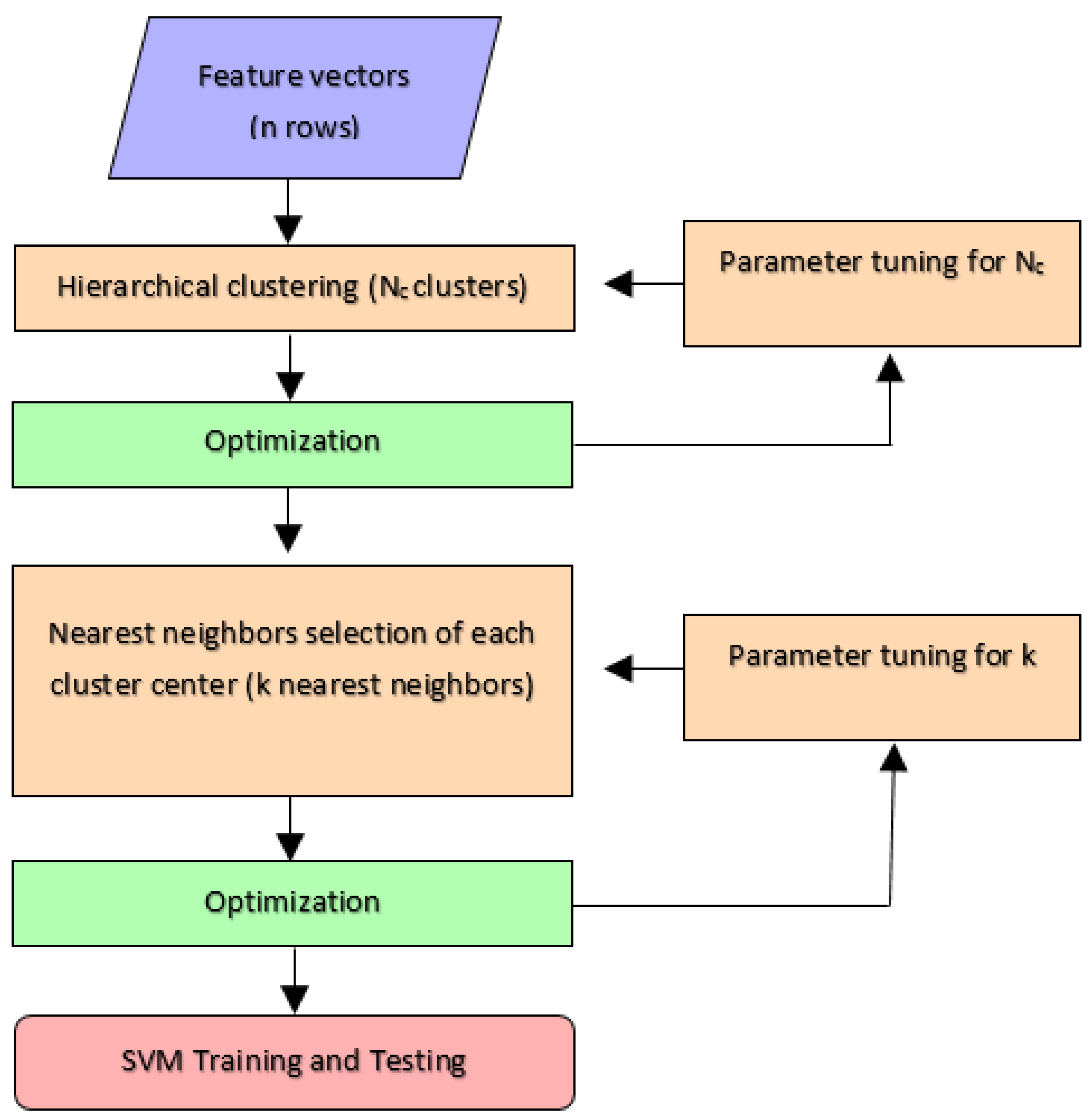
The second method clusters the data samples by a hierarchical clustering algorithm and replaces the train set samples with nearest neighbors of the cluster centers. First, the PSSM feature vectors of the amino acids in train set are clustered using hierarchical clustering algorithm. The number of clusters is denoted as $N_c$. In the next step, k nearest neighbors of each cluster center are selected as the data samples for train set of the SVM classifier. Figure 4 summarizes the steps of sample reduction by clustering procedure. The hyper-parameters $N_c$ and k are optimized by computing the prediction accuracy on validation sets as explained in the next section. Different methods are employed for hierarchical clustering and among those the Ward’s method provided the best results [41]. The Ward’s method applies a minimum variance criterion that minimizes the total within cluster variance. At each step, it finds the pair of clusters that leads to minimum increase in total within-cluster variance after merging. This increase is a weighted square distance between cluster centers. The initial cluster distances are defined to be the squared Euclidean distances between points [41,42].

According to the scipy’s documents, for the Ward’s method, an algorithm called nearest-neighbors chain is implemented which has time complexity $O\left(n^2\right)$. For other methods a naive algorithm is implemented with $O\left(n^3\right)$ time complexity. All algorithms use $O\left(n^2\right)$ memory [43,44].

3.6. Cross-Validation and Hyper-Parameter Optimization for Clustering

The accuracy of data reduction strategies is evaluated in a cross-validation setting. For this purpose, proteins in CB513 are randomly assigned to seven folds and the train/test splits are formed accordingly. This results in a total of seven train test set pairs. For instance, in the first train set there are a total of 73,622 amino acid samples 34.70% (25,544) of which belong to helix, 22.26% (16,387) to beta strand and 43.04% (31,691) to loop. Based on this assignment, there remains a total of 10.497 amino acids for the first test set. In train and test sets, each amino acid is represented by a total of 539 features.

The number of clusters and number of nearest neighbours, which are hyper-parameters of the “sample reduction by hierarchical clustering” approach are optimized by performing a grid search. The first hyper-parameter of $N_c$ represents the number of clusters. To optimize this parameter, values ranging from 500 to 1500 are considered. The second hyper-parameter k is the number of nearest neighbors, which is also optimized by choosing values from 1 to 19. For this purpose, approximately 10% of the proteins from each train set are randomly selected and a total of seven validation sets are formed. Note that the validation sets are used as secondary test sets to optimize the hyper-parameters. The reason for selecting 10% of the train set is to allow as many samples as possible in the train set so that the prediction accuracy is not affected. In selecting validation sets stratified random selection is not performed because the there is not a large imbalance between different class types. Once validation sets are formed, the remaining samples are used to train the SVM models and prediction accuracies are computed on validation sets for different values of the hyper-parameters. Then the parameters with the best validation set accuracy are selected for each iteration of the cross-validation experiment. Once the optimum hyper-parameters are found (a total of seven optimum parameter pairs), the SVM is trained on the original train sets and predictions are computed on test sets.

3.7. System Architecture and Hyper-Parameters of the SVM

The SVM with RBF kernel, which provides satisfactory results for protein secondary structure prediction is implemened using the libSVM software (version 3.21). The hyper-parameters of the SVM are selected as $\alpha$ = 0.00781 and C = 1.0, which have been optimized previously by Aydin et al. [9]. The methods are implemented on a Centos Enterprise Linux 7.3 OS, with an 8 × 2 CPU (CPU/GPU), Intel(R) Xeon(R) E5-2690 processor, 2.90 GHz CPU and 256GB RAM as well as on Ubuntu 16.04.2 LTS (Xenial Xerus) OS, with an Intel(R) Xeon(R) CPU E5-2650 v2 @ 2.60GHz and 64GB RAM.

4. Results

4.1. Sample Reduction by Stratified Random Selection

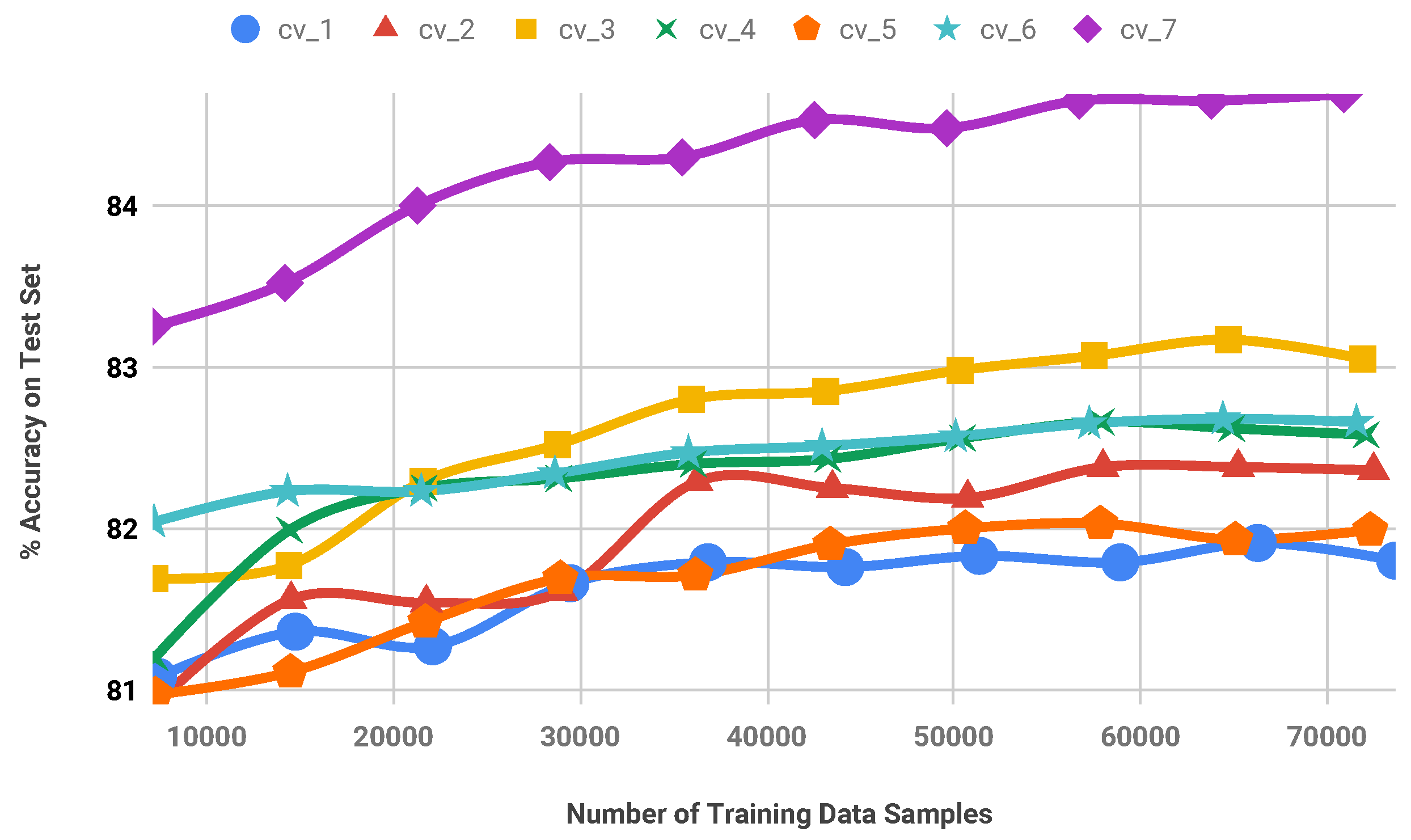
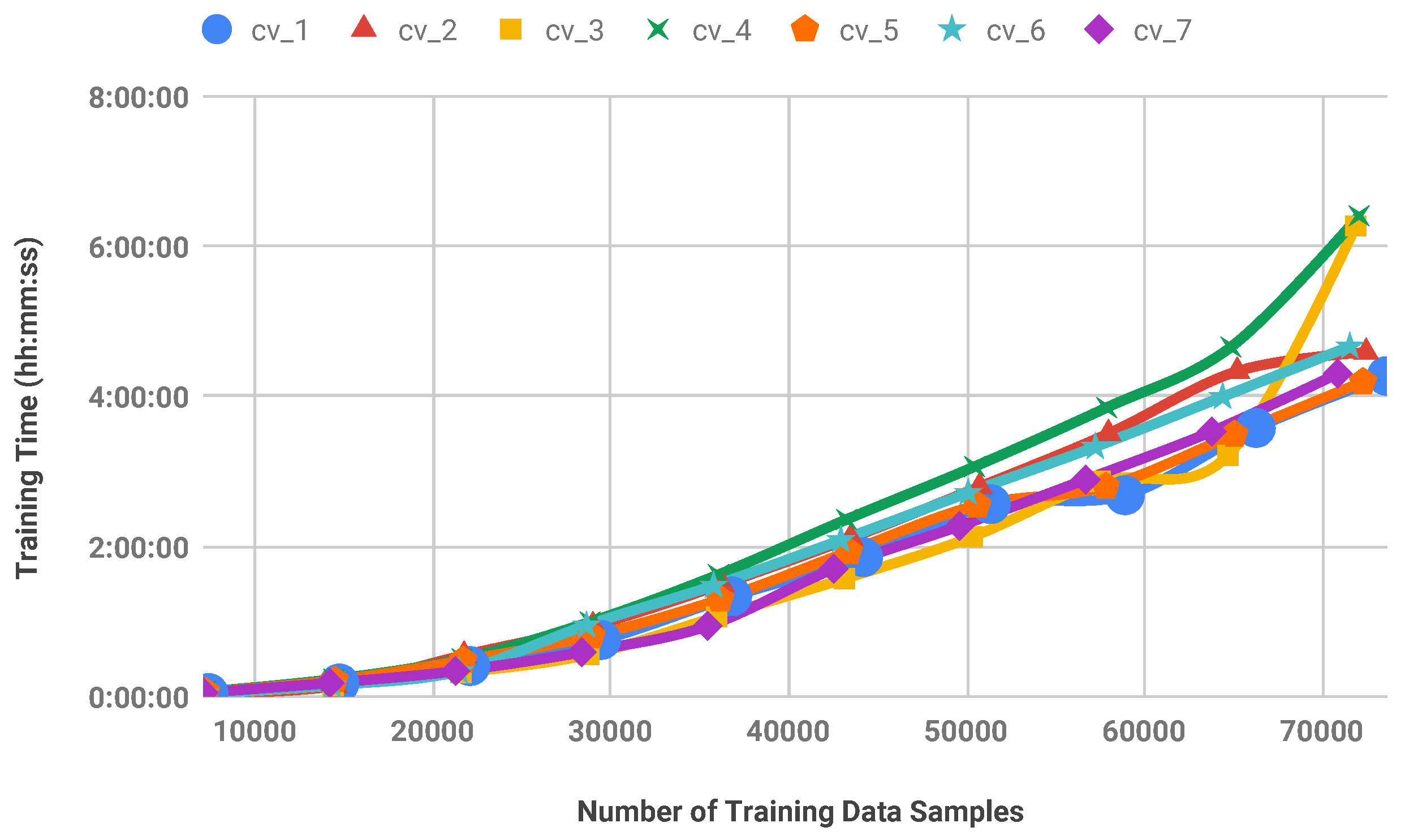
Stratified random selection is performed for each train set of the 7-fold cross-validation experiment. For this purpose, a fixed percentage of amino acid samples are selected randomly from the train set using stratified sampling and the SVM model is trained on this reduced set. In the next step, predictions are computed on the test sets. Figure 5 and Figure 6 show the secondary structure prediction accuracy of the SVM classifier as well as model training times, respectively for all folds of the cross-validation. According to these results, it is possible to remove approximately 50% of data samples from the train sets of CB513 without decreasing the prediction accuracy significantly. Note that the obtained accuracy values are comparable to the state-of-the-art accuracy on CB513 benchmark [11]. Furthermore, the model training time of the SVM is decreased by 73.38% when the training set is reduced by 50% to contain approximately 36,000 amino acid samples only.

Table 1. Overall prediction accuracies of the stratified random selection method using the various training samples and k-fold (k = 7) cross-validation.

D	CV-Fold 1				CV-Fold 2				CV-Fold 3				CV-Fold 4
	$\mathit{S}$	${\mathit{Acc}}_{\mathit{p}}$	${\mathit{Time}}_{\mathit{t}}$	${\mathit{Time}}_{\mathit{p}}$	$\mathit{S}$	${\mathit{Acc}}_{\mathit{p}}$	${\mathit{Time}}_{\mathit{t}}$	${\mathit{Time}}_{\mathit{p}}$	$\mathit{S}$	${\mathit{Acc}}_{\mathit{p}}$	${\mathit{Time}}_{\mathit{t}}$	${\mathit{Time}}_{\mathit{p}}$	$\mathit{S}$	${\mathit{Acc}}_{\mathit{p}}$	${\mathit{Time}}_{\mathit{t}}$	${\mathit{Time}}_{\mathit{p}}$
10	7362	81.0803	00:02:55	00:46	7246	80.9144	00:02:19	00:46	7188	81.6860	00:02:20	00:48	7207	81.2044	00:04:03	01:15
20	14,724	81.3566	00:10:32	01:22	14,492	81.5577	00:08:26	01:20	14,375	81.7677	00:08:57	01:28	14,413	81.9924	00:14:00	02:04
30	22,087	81.2708	00:24:26	02:31	21,738	81.5406	00:33:08	03:08	21,563	82.2905	00:19:09	01:55	21,619	82.2495	00:30:18	02:52
40	29,449	81.6614	00:45:17	03:17	28,984	81.6092	00:56:39	03:37	28,751	82.5192	00:33:35	02:25	28,825	82.3076	00:59:44	04:49
50	36,811	81.7853	01:20:09	03:24	36,231	82.2868	01:29:45	04:04	35,939	82.7969	01:03:47	03:32	36,032	82.3988	01:37:28	05:09
60	44,173	81.7567	01:51:31	04:07	43,477	82.2525	02:06:47	04:48	43,126	82.8459	01:34:15	04:04	43,238	82.4320	02:21:37	05:05
70	51,353	81.8329	02:33:51	04:00	50,723	82.1925	02:47:47	05:14	50,314	82.9848	02:07:46	04:52	50,444	82.5647	03:03:54	05:32
80	58,898	81.7948	02:41:01	04:26	57,969	82.3812	03:30:18	05:41	57,502	83.0665	02:52:04	05:36	57,872	82.6642	03:51:04	06:05
90	66,260	81.9091	03:34:47	04:50	65,215	82.3812	04:20:07	06:11	64,689	83.1727	03:12:45	05:33	64,857	82.6228	04:39:29	06:34
100	73,622	81.8043	04:16:21	04:59	72,461	82.3555	04:35:17	06:44	71,877	83.0502	06:16:19	09:59	72,063	82.5813	06:24:23	08:42
D	CV-Fold 5				CV-Fold 6				CV-Fold 7
	$\mathit{S}$	${\mathit{Acc}}_{\mathit{p}}$	${\mathit{Time}}_{\mathit{t}}$	${\mathit{Time}}_{\mathit{p}}$	$\mathit{S}$	${\mathit{Acc}}_{\mathit{p}}$	${\mathit{Time}}_{\mathit{t}}$	${\mathit{Time}}_{\mathit{p}}$	$\mathit{S}$	${\mathit{Acc}}_{\mathit{p}}$	${\mathit{Time}}_{\mathit{t}}$	${\mathit{Time}}_{\mathit{p}}$
10	7228	80.9697	00:03:41	01:09	7154	82.0372	00:02:33	00:51	7087	83.2541	00:03:16	01:08
20	14,456	81.1133	00:12:58	01:56	14,309	82.2281	00:09:09	01:33	14,173	83.5182	00:10:53	01:47
30	21,684	81.4173	00:02:58	02:38	21,463	82.2281	00:20:14	02:08	21,260	84.0012	00:20:23	02:20
40	28,912	81.6876	00:48:29	03:16	28,618	82.3394	00:57:00	04:15	28,347	84.2729	00:35:28	02:53
50	36,140	81.7130	01:17:51	04:00	35,772	82.4666	01:28:50	04:30	35,435	84.2955	00:56:28	03:16
60	43,368	81.8988	01:55:50	04:34	42,925	82.5143	02:05:09	04:43	42,521	84.5295	01:42:06	04:42
70	50,596	82.0002	02:33:00	05:08	50,081	82.5700	02:42:56	05:01	49,608	84.4842	02:16:27	05:14
80	57,824	82.0340	02:47:52	05:19	57,234	82.6495	03:19:41	05:16	56,695	84.6502	02:53:34	05:39
90	65,052	81.9326	03:29:32	05:19	64,390	82.6813	03:59:41	05:37	63,781	84.6502	03:31:57	06:36
100	72,280	81.9917	04:11:39	05:44	71,543	82.6574	04:40:00	05:48	70,868	84.6879	04:18:13	07:17

summarizes the overall prediction accuracies of the stratified random selection method using the various training samples and k-fold (k = 7) cross-validation. In this table, D represents the sampled dataset as a percentage, S represents the randomly and uniquely selected rows, $Ac{c}_p$ denotes the overall accuracy in percentages (i.e., $Q_3$) on validation sets and $Tim{e}_t$ is the training time in hours, minutes and seconds, $Tim{e}_p$ is the prediction time in minutes and seconds.

4.2. Sample Reduction by Hierarchical Clustering

A 7-fold cross-validation on CB513 is also performed for sample reduction by hierarchical clustering method. In each iteration, the samples in the train set are clustered by a hierarchical clustering algorithm and the train samples are replaced with nearest neighbors of the cluster centers. We first optimized the number of clusters and the number of nearest neighbors from each cluster center.

Table 2. Results for sample reduction by Ward’s hierarchical clustering. A seven-fold cross-validation experiment is performed on CB513 benchmark.

CV-Fold	k	${\mathit{N}}_{\mathit{c}}$	${\mathit{N}}_{\mathit{tr}}$	${\mathit{Acc}}_{\mathit{v}}(\%)$	${\mathit{Acc}}_{\mathit{t}}(\%)$
1	13	1500	48,928	83.5473	81.9567
1		all	65,903	83.8700	81.7186
2	17	1500	55,458	81.3475	82.1839
2		all	65,212	81.1100	82.1839
3	17	1100	47,607	84.0580	82.9848
3		all	64,833	83.8733	83.0583
4	17	1400	54,249	83.3821	82.6808
4		all	65,901	83.3983	82.5315
5	17	1500	55,628	84.1406	81.8397
5		all	65,048	84.2652	82.0593
6	17	1500	54,810	81.9583	82.4427
6		all	63428	82.1063	82.6733
7	17	1500	54,330	83.0679	84.8011
7		all	62,517	83.0439	84.7257

summarizes the experimental results obtained by Ward’s hierarchical clustering method. In this table, $N_c$ represents the number of clusters, k represents the number of nearest neighbors from each cluster center, $N_{tr}$ is the number of train set samples, $Ac{c}_v$ denotes the overall accuracy in percentages (i.e., $Q_3$) on validation sets and $Ac{c}_t$ is the overall accuracy on test sets. An $N_c$ value of “all” represents the setting in which all the samples are used for model training (i.e., each sample is assigned to a different cluster). The optimum number of clusters for each fold is 1500 except for the third and fourth folds. Typically, 17 closest samples are selected from each cluster based on the distance from cluster center. At the first fold, 13 closest samples were selected as the optimum number of nearest neighbors. Test set prediction accuracy is obtained as almost identical both on reduced and the whole datasets for each fold of the cross-validation experiment, which is comparable to the state-of-the-art [11]. Data in the training set are preprocessed before inputting to the SVM in order to improve the training time. As a result of these experiments clustering approach can reduce the train set size by 26% without reducing the prediction accuracy significantly.

In addition to prediction accuracy, it is of interest to analyze the running time of the sample reduction by hierarchical clustering method and the running time of the SVM classifier with and without clustering applied. For this purpose the following experiment is performed on the first fold of the seven-fold cross-validation experiment. The number of clusters $N_c$ is set to 1000 and the number of nearest neighbors k to 13, which resulted in 36,622 training examples for the SVM. The running times are obtained for each step as follows. Hierarchical clustering: 14.51 s, finding the $k=13$ nearest neighbors of cluster centers: 59.25 s, training of SVM using 36,622 samples: 6 h, 16 min and 43 s. The total running time of the sample reduction by hierarchical clustering approach is obtained as 6 h, 17 min and 56 s. When the SVM is trained using all of the samples in the first fold’s training set it took 14 h, 10 min and 22 s. Based on these results, it can be stated that the running time of sample reduction by hierarchical clustering followed by SVM training is typically lower than training the SVM using the full training set.

4.3. Average Accuracies

Table 3. Average and standard deviation of test accuracies obtained for the 7-folds of cross-validation experiment on CB513.

Method	${\mathit{Acc}}_{\mathit{t}}(\%)$	$\mathit{std}\left({\mathit{Acc}}_{\mathit{t}}\right)$
Sample reduction by random selection	82.728	0.947
Sample reduction by hierarchical clustering	81.825	1.285
No sample reduction	82.732	0.958

summarizes the average and standard deviation of the accuracies obtained from the 7 folds of cross-validation experiment on CB513. In this table the first two rows include the results obtained for the sample reduction strategies and the last row represents the case where all samples are used to train the SVM classifier. Having low standard deviation values demonstrates that the accuracy evaluations are robust and models are trained with sufficiently large samples. To assess whether the difference between the accuracy values of sample reduction methods and the method that uses all samples is statistically significant, a two-tailed Z-test is performed with a confidence value of 95%. Based on this test, the accuracy difference between sample reduction by stratified random selection and the method that uses all samples is not found to be statistically significant with a Z-score of −0.0217 and a p-value of 0.98404. On the other hand, the accuracy difference between sample reduction by clustering and the method that uses all samples is statistically significant with a Z-score of −4.8713 and a p-value < 1 $\times {10}^{-5}$. Based on these results, it can be concluded that sample reduction by stratified random sampling is more effective than sample reduction by hierarchical clustering approach for protein secondary structure prediction.

5. Conclusions

In this paper, we proposed two data reduction strategies for improving the model training time of a support vector machine classifier. The proposed solutions can reduce the dataset size by 26–50% up to approximately 36,000 amino acid samples. The accuracy evaluations are performed by doing cross-validation experiments on CB513 benchmark. For larger datasets, it can still be sufficient to keep approximately 36,000 samples in train set to get satisfactory prediction accuracy, which may correspond to removing even higher percentage of data samples from the train set. This will be investigated further as a future work. Additionally, de-clustering strategies can be implemented and the clusters can be expanded mainly around the decision boundaries. This will provide a finer grained expansion of clusters on regions where the classifier has the most confusion. As a third direction, a smaller train set can be formed for each test example using the cluster centers as guides.

References

- Liu, Y. Conditional Graphical Models for Protein Structure Prediction. Ph.D. Thesis, Carnegie Mellon University, Pittsburgh, PA, USA, 2006. [Google Scholar]
- Protein Structure. Available online: https://www.wikizeroo.org/index.php?q=aHR0cHM6Ly9lbi53aWtpcGVkaWEub3JnL3dpa2kvUHJvdGVpbl9TdHJ1Y3R1cmU (accessed on 10 April 2018).
- Devi, L.; Mansi, V. Large-Scale Sequence Comparison; Humana Press: New York, NY, USA, 2017; pp. 191–224. [Google Scholar]
- Rost, B. Protein Secondary Structure Prediction Continues to Rise. J. Struct. Biol. 2001, 134, 204–218. [Google Scholar] [CrossRef] [PubMed]
- Whisstock, J.C.; Lesk, A.M. Prediction of protein function from protein sequence and structure. Q. Rev. Biophys. 2003, 36, 307–340. [Google Scholar] [CrossRef] [PubMed]
- Holley, L.H.; Karplus, M. Protein secondary structure prediction with a neural network. Proc. Nalt. Acad. Sci. USA 1989, 86, 152–156. [Google Scholar] [CrossRef] [PubMed]
- Pollastri, G.; Mclysaght, A. Structural bioinformatics Porter: A new, accurate server for protein secondary structure prediction. Bioinformatics 2004, 21, 1719–1720. [Google Scholar] [CrossRef] [PubMed]
- Mandle, A.K.; Jain, P.; Shrivastava, S.K. Protein structure predictions usign support vector machine. Int. J. Soft Comput. 2012, 3, 67–78. [Google Scholar] [CrossRef]
- Aydin, Z.; Singh, A.; Bilmes, J.; Noble, W.S. Learning sparse models for a dynamic Bayesian network classifier of protein secondary structure. BMC Bioinform. 2011, 12, 154. [Google Scholar] [CrossRef] [PubMed]
- Wang, S.; Peng, J.; Ma, J.; Xu, J. Protein secondary structure prediction usign deep convolutional neural fields. Sci. Rep. 2016, 6, 18962. [Google Scholar] [CrossRef]
- Aydin, Z.; Kaynar, O.; Gormez, Y. Dimensionality reduction for protein secondary structure and solvent accessibility prediction. J. Bioinform. Comput. Biol. 2018, 16, 1850020. [Google Scholar] [CrossRef]
- Mirdita, M.; von den Driesch, J.; Galiez, C.; Martin, M.J.; Söding, H.; Steinegger, M. Uniclust databases of clustered and deeply annotated protein sequences and alignments. Nucleic Acids Res. 2017, 45, D170–D176. [Google Scholar] [CrossRef]
- Remmert, M.; Biegert, A.; Hauser, A. HHblits: Lightning-fast iterative protein sequence searching by HMM-HMM alignment. Nat. Methods 2012, 9, 173. [Google Scholar] [CrossRef]
- Lo Conte, L.; Ailey, B.; Hubbard, T.J.P.; Brenner, S.E.; Murzin, A.G.; Chothia, C. SCOP: A Structural Classification of Proteins database. Nucleic Acids Res. 2002, 28, 257–259. [Google Scholar] [CrossRef] [PubMed]
- Bateman, A.; Birney, E.; Cerruti, L.; Durbin, R.; Etwiller, L.; Eddy, S.E.; Griffiths-Jones, S.; Howe, K.L.; Marshall, M.; Sonnhammer, E.L.L. The Pfam Protein Families Database. Nucleic Acids Res. 2002, 30, 276–280. [Google Scholar] [CrossRef] [PubMed] [Green Version]
- Aydin, Z.; Kaynar, O.; Gormez, Y.; Isik, E.Y. Comparison of machine learning classifiers for protein secondary structure prediction. In Proceedings of the IEEE 26th Signal Processing and Communication Applications Conference (SIU), Izmir, Turkey, 2–5 May 2018; pp. 1–4. [Google Scholar]
- Cortes, C.; Vapnik, V. Support-Vector Networks. Mach. Learn. 1995, 20, 273–297. [Google Scholar] [CrossRef]
- Jun, S. Support Vector Machine based on Stratified Sampling. Int. J. Fuzzy Logic Intell. Syst. 2009, 9, 141–146. [Google Scholar] [CrossRef] [Green Version]
- Awad, M.; Khan, L.; Bastani, F.; Yen, I.L. An effective support vector machines (SVMs) performance using hierarchical clustering. In Proceedings of the 16th IEEE International Conference on Tools with Artificial Intelligence, Boca Raton, FL, USA, 15–17 November 2004; pp. 663–667. [Google Scholar]
- Yu, H.; Yang, J.; Han, J. Classifying large data sets using SVMs with hierarchical clusters. In Proceedings of the Ninth ACM SIGKDD International Conference on Knowledge Discovery and Data, Mining, KDD ’03, Washington, DC, USA, 24–27 August 2003; p. 306. [Google Scholar]
- Blachnik, M. Reducing time complexity of svm model by lvq data compression. In International Conference on Artificial Intelligence and Soft Computing; Springer: Cham, Switzerland, 2015; pp. 687–695. [Google Scholar]
- Xie, S.; Li, Z.; Hu, H. Protein secondary structure prediction based on the fuzzy support vector machine with the hyperplane optimization. Gene 2018, 642, 74–83. [Google Scholar] [CrossRef]
- Lin, L.; Yang, S.; Zuo, R. Protein secondary structure prediction based on multi-SVM ensemble. In Proceedings of the 2010 International Conference on Intelligent Control and Information Processing, Dalian, China, 13–15 August 2010; pp. 356–358. [Google Scholar]
- Hua, S.; Sun, Z. A novel method of protein secondary structure prediction with high segment overlap measure: Support vector machine approach. J. Mol. Biol. 2001, 308, 397–407. [Google Scholar] [CrossRef]
- Hens, A.B.; Tiwari, M.K. Computational time reduction for credit scoring: An integrated approach based on support vector machine and stratified sampling method. Expert Syst. Appl. 2012, 39, 6774–6781. [Google Scholar] [CrossRef]
- Cuff, J.A.; Barton, G.J. Evaluation and improvement of multiple sequence methods for protein secondary structure prediction. Proteins Struct. Funct. Genet. 1999, 34, 508–519. [Google Scholar] [CrossRef] [Green Version]
- Guo, J.; Chen, H.; Sun, Z.; Lin, Y. A novel method for protein secondary structure prediction using dual-layer SVM and profiles. Proteins Struct. Funct. Bioinform. 2004, 54, 738–743. [Google Scholar] [CrossRef]
- Kabsch, W.; Sander, C. Dictionary of protein secondary structure: Pattern recognition of hydrogen-bonded and geometrical features. Biopolym. Orig. Res. Biomol. 1983, 22, 2577–2637. [Google Scholar] [CrossRef]
- Berman, H.; Henrick, K.; Nakamura, H. Announcing the worldwide Protein Data Bank. Nat. Struct. Biol. 2003, 10, 980. [Google Scholar] [CrossRef] [PubMed]
- Zhu, X.J.; Feng, C.Q.; Lai, H.Y.; Chen, W.; Hao, L. Predicting protein structural classes for low-similarity sequences by evaluating different features. Knowl.-Based Syst. 2019, 163, 787–793. [Google Scholar] [CrossRef]
- Altschul, S.F.; Madden, T.L.; Schäffer, A.A.; Zhang, J.; Zhang, Z.; Miller, W.; Lipman, D.J. Gapped BLAST and PSI-BLAST: A new generation of protein database search programs. Nucleic Acids Res. 1997, 25, 3389–3402. [Google Scholar] [CrossRef] [PubMed]
- NCBI: National Center for Biotechnology Information. Available online: ncbi.nlm.nih.gov/ (accessed on 5 April 2018).
- PDB70 Database. Available online: wwwuser.gwdg.de/~compbiol/data/hhsuite/databases/hhsuite_dbs/old-releases/ (accessed on 23 September 2019).
- Görmez, Y. Dimensionality Reduction for Protein Secondary Structure Prediction; Abdullah Gul University: Kayseri, Turkey, 2017. [Google Scholar]
- Aydin, Z.; Baker, D.; Noble, W.S. Constructing structural profiles for protein torsion angle prediction. In Proceedings of the International Joint Conference on Biomedical Engineering Systems and Technologies, Lisbon, Portugal, 12–15 January 2015; SCITEPRESS-Science and Technology Publications, Lda.: Lisbon, Portugal, 2015; Volume 3, pp. 26–35. [Google Scholar]
- Vapnik, V.N. Statistical Learning Theory. Adapt. Learn. Syst. Signal Process. Commun. Control 1998, 2, 1–740. [Google Scholar]
- Gunn, S.R. Support Vector Machines for Classification and Regression. ISIS Tech. Rep. 1998, 14, 5–16. [Google Scholar]
- Vert, J.-P. Kernel methods in genomics and computational biology. arXiv 2005, arXiv:q-bio/0510032. [Google Scholar]
- Cortes, C. Prediction of Generalization Ability in Learning Machines. Ph.D. Thesis, University of Rochester, New York, NY, USA, 1995. [Google Scholar]
- Zhang, Q.; Wang, H.; Yoon, S.W. A Hierarchical Feature Selection Model using Clustering and Recursive Elimination Methods. In Proceedings of the 2017 Industrial and Systems Engineering Research Conference, Pittsburgh, PA, USA, 20–23 May 2017. [Google Scholar]
- Ward, J.H., Jr. Hierarchical grouping to optimize an objective function. J. Am. Stat. Assoc. 1963, 58, 236–244. [Google Scholar] [CrossRef]
- Ward’s Method. Available online: https://en.wikipedia.org/wiki/Ward%27s_method (accessed on 23 September 2019).
- Müllner, D. Modern hierarchical, agglomerative clustering algorithms. arXiv 2011, arXiv:1109.2378. (In Preprint) [Google Scholar]
- SciPy. Available online: https://docs.scipy.org/doc/scipy/reference/generated/scipy.cluster.hierarchy.linkage.html (accessed on 23 September 2019).
Figure 1.
Definition of protein secondary structure prediction problem.
Figure 2.
A structural profile matrix for protein secondary structure prediction.
Figure 3.
The steps of the DSPRED method.