Multi-Robot Exploration Based on Multi-Objective Grey Wolf Optimizer


1
Department of Electrical Engineering, Yeungnam University, Gyeongsan 38541, Korea
2
School of Control and Computer Engineering, North China Electric Power University, Beijing 102206, China
*
Author to whom correspondence should be addressed.
Appl. Sci. 2019, 9(14), 2931; https://doi.org/10.3390/app9142931
Submission received: 25 June 2019
/
Revised: 17 July 2019
/
Accepted: 17 July 2019
/
Published: 22 July 2019
(This article belongs to the Special Issue Mobile Robots Navigation)
Abstract
:In this paper, we used multi-objective optimization in the exploration of unknown space. Exploration is the process of generating models of environments from sensor data. The goal of the exploration is to create a finite map of indoor space. It is common practice in mobile robotics to consider the exploration as a single-objective problem, which is to maximize a search of uncertainty. In this study, we proposed a new methodology of exploration with two conflicting objectives: to search for a new place and to enhance map accuracy. The proposed multiple-objective exploration uses the Multi-Objective Grey Wolf Optimizer algorithm. It begins with the initialization of the grey wolf population, which are waypoints in our multi-robot exploration. Once the waypoint positions are set in the beginning, they stay unchanged through all iterations. The role of updating the position belongs to the robots, which select the non-dominated waypoints among them. The waypoint selection results from two objective functions. The performance of the multi-objective exploration is presented. The trade-off among objective functions is unveiled by the Pareto-optimal solutions. A comparison with other algorithms is implemented in the end.
1. Introduction
In robotics, exploration pertains to the process of scanning and mapping out an environment to produce a map, which can be used by a robot or group of robots for further work. Based on the type of environment, exploration can be one of the following: outdoor, indoor, or underwater, using a mobile-robot or multi-robot systems [1,2]. In this study, we focused on indoor exploration by robots, which are equipped with ranging sensors. It can be assumed that these robots with onboard sensors can scan an environment without any difficulties by walking randomly around. However, their motion is not efficient, which can result in an incomplete map coverage. As a solution to this issue, this paper proposes an algorithm that enhances the efficiency of the multi-robot exploration by using a multi-objective optimization strategy.
Naturally, all real-world optimization problems in engineering pursue multiple goals. They may differ from each other in various fields. However, it is common for all to optimize problems by maximization or minimization functions. In the past, multiple optimization problems were solved by one function because of the lack of suitable solution methodologies for solving a multi-objective optimization problem (MOOP) as a single-objective optimization problem. With the development of evolutionary algorithms, new techniques, which seek to optimize two or more conflicting objectives in one simulation run, have been applied to MOOPs. This new research area is named multi-objective optimization (MOO) [3].
In robotics, studies related to optimization have been gaining wide attention [4]. If we consider multi-robot systems [5], optimization is popularly applied in path planning [6], formation [7], exploration [8], and other fields where decision-making control needs to be optimized. Previous research conventionally found the optimal solutions as separated single-objective tasks: short path, obstacle-free motion, smoothest route, and constant search of uncertain terrain. The new impact of optimization in robotics is obtained due to the metaheuristics and its nature-inspired optimization techniques [9]. The nature-inspired algorithms are not only restricted to robotics but also have significant applications in different fields. Due to this, they have attracted the attention of scholars [10,11].
Metaheuristic algorithms are optimization approaches, which emulate the intelligence of various species of animals in nature. The number of agents classifies the metaheuristic algorithms into single-solution-based and population-based algorithms. In both classes, the solutions improve over the course of iterations with one single agent or an entire swarm of agents, respectively. The main advantage of population-based approaches is their ability to avoid stagnation in the local optima due to the number of agents. The swarm can explore search space more and faster than a single agent. Regardless of this, the benefit of one class over the other depends on its application in a certain problem. However, it is important to mention the No-Free-Lunch (NFL) theorem for optimization, which assures that there is no algorithm with universal optimal solution by all criteria and in all domains [12].
Despite the number of agents, the metaheuristic algorithms can be classified into single and multi-objective optimization techniques according to the number of objective functions. A multi-objective optimization is an extended approach to single optimization. It allows finding an optimal solution of two independent objectives simultaneously. In order to select just one best solution from the available ones, a trade-off should be considered among them. The Pareto-optimal front helps pick up one of the suitable solutions satisfying two objective functions.
Examples of the single-objective algorithms include the Particle Swarm Optimization (PSO) [13], Genetic Algorithm (GA) [14], Ant Colony Optimization (ACO) [15], Grey Wolf Optimizer algorithms (GWO) [16,17], which have the extended multi-objective optimization variations, namely MOPSO [18], MOGA [19], m-ACO [20], and MOGWO [21], respectively. In our previous study [8], we used the coordinated multi-robot exploration [22] and GWO algorithms together as a hybrid. In this study, our interest is to solve the multi-robot exploration problem as the MOOP using Multi-Objective Grey Wolf Optimizer (MOGWO).
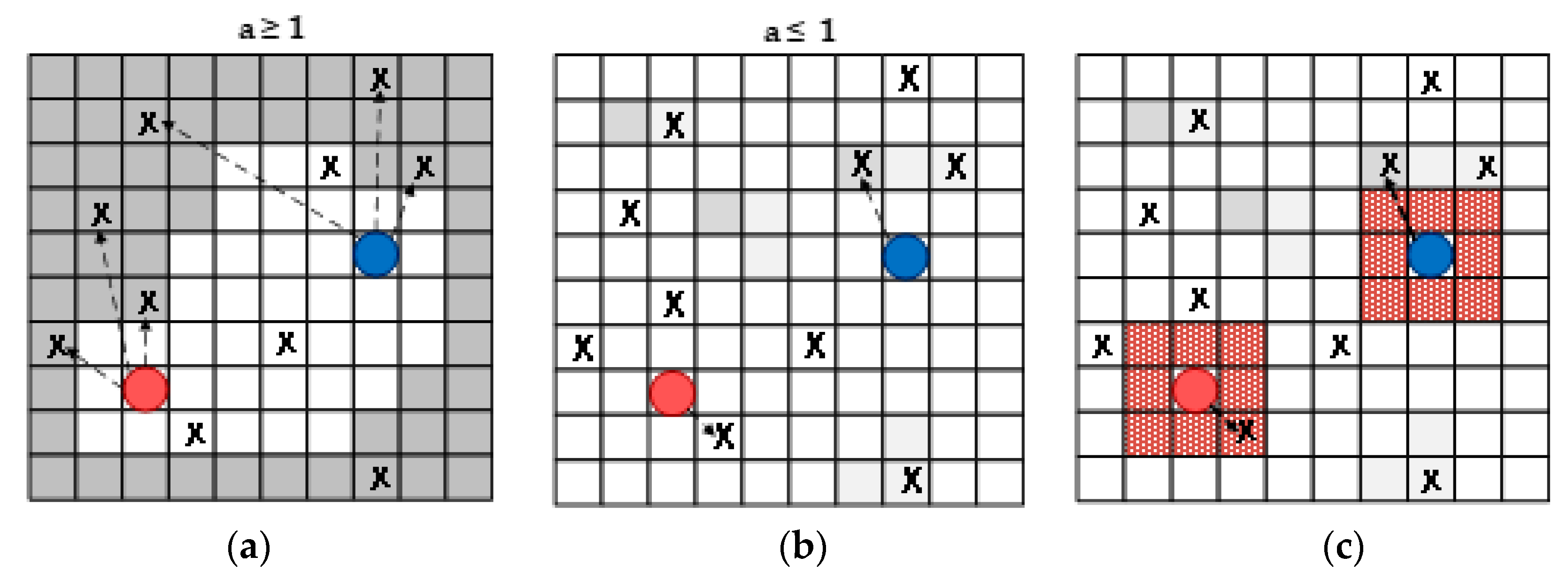
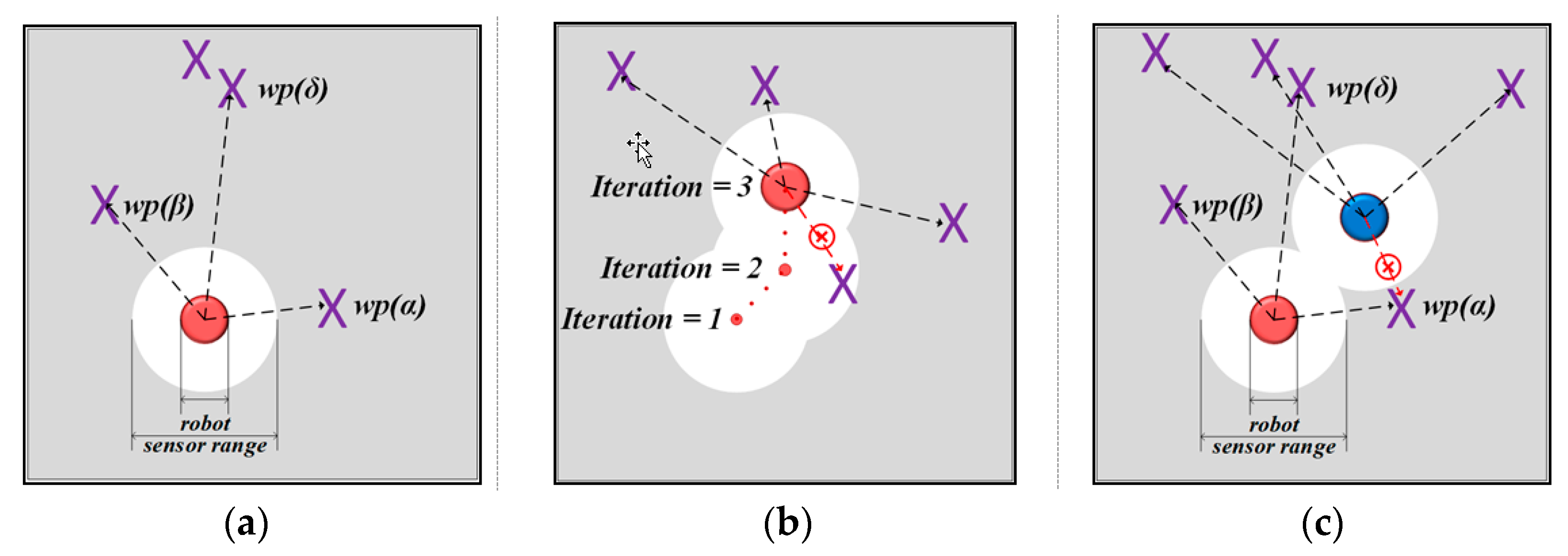
Using the MOGWO exploration, we defined two objectives for optimization, namely the maximization of the search for new area and the minimization of the inaccuracy of the explored map. It can be said that the search process is divided into two stages (Figure 1). They switch during the simulation run depending on the value of the GWO parameter. If the value is greater than one, it searches occluded space. If the value is less than one, it increases the map accuracy by repeated visits in the explored space. It needs to be emphasized that the occupancy grid map with probabilistic values is used in this study [23].
The MOGWO exploration employs static waypoints in the simulation, which promotes the efficient exploration of an indoor simulated environment. It can be noted that the waypoints belong to the programmed logic of the algorithm and are not supposed to be used in the real environment [24]. The waypoints are grey wolf agents with some costs of probability values. In each iteration, the robots search alpha, beta, and gamma waypoints and save them in an archive wherein avoiding the selection the same non-dominated waypoints for several robots. After the selection, the robots can compute the next position, which is the closest to the average position of alpha, beta, and gamma waypoints, from among the frontier cells [25].
This paper is organized as follows: in Section 2, we briefly recall different algorithms of multi-robot exploration and evolutionary optimization techniques used in related works. In Section 3, the theory of GWO and MOGWO is presented. Section 4 and Section 5 are dedicated to the proposed MOGWO exploration and its performance. Section 6 concludes the present study.
2. Related Work
In the last two decades, many techniques have been proposed for robot exploration. Among them, there are novel fundamental, hybridized, and modified methods. In this section, studies on the different algorithms and the impact of the evolutionary optimization techniques in exploration are discussed.
Considering exploration as one of the branches in robotics, Yamauchi et al.’s frontier-based method is the pioneering work in this field [26]. From that time up to now, many frontier-based studies have appeared, most of which were hybridized or modified with success.
The coordinated multi-robot exploration (CME) is frontier-based with the emphasis on the cooperative work with a team of robots [22]. The robot’s mission is to search for maximum utility with the minimum cost that diverges the robots from each other keeping the direction to search unexplored space. The alternative coordinated method is the randomized graph approach [27,28]. It builds a roadmap in an explored area that navigates robots to move through safe paths. Recently, Alfredo et al. [29] introduced the efficient backtracking concept to the random exploration graph, preventing the same robot in visiting the same place more than once. These above-mentioned methods have the common idea of using frontier-based control.
Another approach in exploration that is completely different in theory and practice is artificial intelligence (AI). Reinforcement Learning (RL) and convolutional neural network (CNN) are such attempts, which have been proposed in previous studies [30,31,32]. The exploration-based approach on neural networks differs considerably from the frontier-based approach in terms of environment perception and control system. Visual sensors (cameras) scan a place for further computation using image-processing algorithms [33]. The output of the calculation is the interaction of the robot with the environment. Lei Tai et al. [34] conducted a survey of leading studies in mobile robotics using deep learning from perception to control systems.
Recently, a novel branch of exploration that employs nature-inspired optimization techniques has appeared. The approaches seek to enhance existing solutions to exploration. Sharma S. et al. [35] applied clustering-based distribution and bio-inspired algorithms such as PSO, Bacteria Foraging Optimization, and Bat algorithm. The clustering provides a direction of robot motion, while the nature-inspired approaches involve exploring the unknown area. The study of [36] applied a combination of PSO, fractional calculus, and fuzzy inference system. They compared their results with other six other PSO variations that showed effective multi-robot exploration. A similar waypoint concept in our study was performed in [37]. The artificial pheromone and fuzzy controllers help the multi-robot systems to navigate efficiently by distributing the search between robots and avoiding repeated visits in explored regions.
The study of [38] involved more than one optimization problem in the exploration, which is important to highlight here. The optimal solution seeks to minimize two objective functions: the variance of path lengths and the sum of the path lengths of all robots. Compared to our research, they applied the K-Means clustering algorithm instead of the bio-inspired technique used in our study.
The study of [39] presented the auto-adaptive multi-objective strategy for multi-robot exploration, where the multi-objective concept consisted of two missions: a search of uncertainties and stable communication. This work is closely related to the present work, but the focus of their research is an assessment of the communication conditions for providing efficient map coverage, which is a different perspective compared to our study.
In regard to multi-objective optimization in multi-robot systems, MOPSO [40] and multi-ACO [41] have already been applied to path planning problem. Broadly speaking, the metaheuristic algorithms are often applied in path planning problems compared to other issues, mainly, because optimization is the core study for finding a short and smooth path.
In general, MOGWO has never been applied before in mobile robotics studies.
3. Single and Multi-Objective Grey Wolf Optimizer
The section briefly describes the theories of GWO and MOGWO. The two techniques have the interconnection that one is inferred to another. Firstly, GWO will be presented, and then, the concept will be extended to the multi-objective optimization using MOGWO.
3.1. Grey Wolf Optimizer
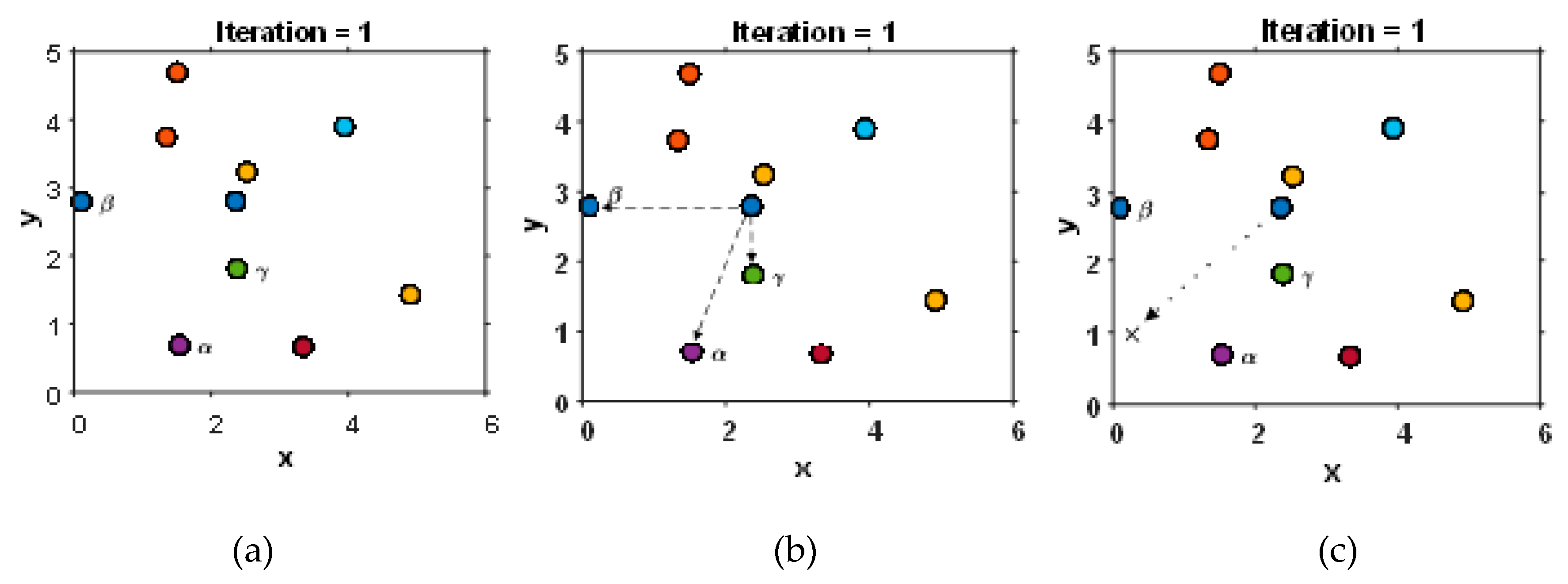
GWO is a population-based metaheuristic algorithm, which mimics the wolf hunting process. Population- and single-based optimization algorithms differ from each other in the number of agents used to carry out a search of a global optimum. Each agent is a candidate for finding a global optimum. Figure 2 shows the GWO simulation. The search begins when all agents obtain random values, where . Then, the cost function defines the best candidates among them in each iteration (Figure 2a) by equation:
Every single agent needs to compute , and then, can be found. The random and adaptive vectors, and are upgraded in each iteration.
Finally, the next agent’s position is mean value of , which Figure 2c is illustrated.
The same calculation will be repeated in each run time for every search agent.
Depending on the values of the vectors, and , also denoted as GWO parameters, the two phases make the transition between divergence (exploration) and convergence (exploitation) in the optimal solution search. The GWO parameters are calculated as follows:
where the value of decreases linearly from 2 to 0 using the update equation for iteration :
and and are random values ranging from 0 to 1.
In GWO, the parameter determines the exploration and exploitation in searching behavior. Each agent of the population performs divergence when and executes convergence from agents when . Figure 2 illustrates how the agent largely changes the next position at iterations t and t+1 by the divergence of the parameter , which is linearly decreasing.
The parameter randomly determines the exploration or exploitation tendencies without dependency on the iterations. The stochastic mechanism in GWO allows the enhanced search of optimality by reaching different positions around the best solutions.
In recent years, the GWO algorithm has been widely modified in various studies. In study [42], the authors improved the convergence speed of GWO by guiding the population using the alpha solution. In another study [43], the new operator called reflecting learning was introduced in the algorithm. It improves the search ability of GWO by the principle of light reflection in physics. The optimization was enhanced in studies [44,45,46] by random walk strategies and Levy flights distribution as well.
3.2. Multi-Objective Grey Wolf Optimizer
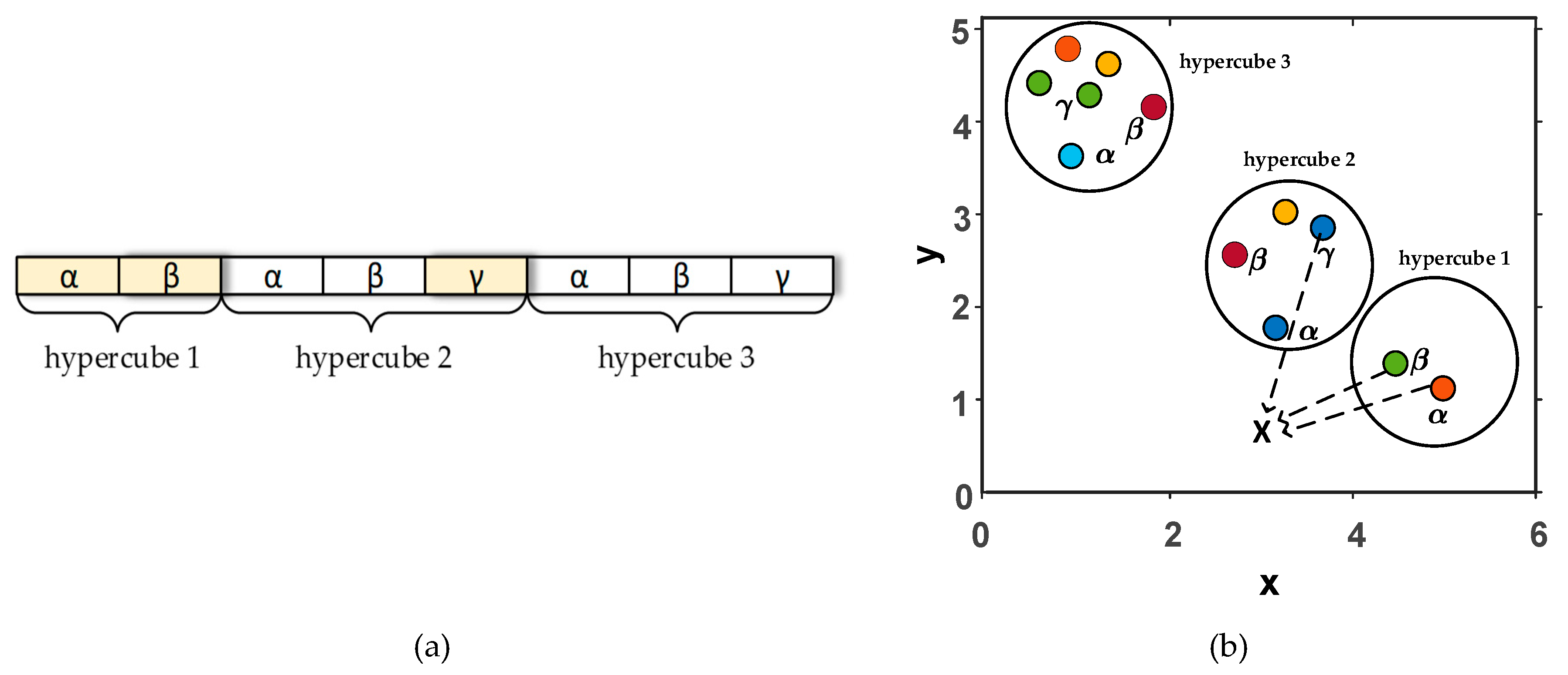
Two new components were integrated into MOGWO for performing multi-objective optimization: an archive of the best non-dominated solutions and a leader selection strategy of alpha, beta, and gamma solutions. The archive is needed for storing non-dominated Pareto solutions through the course of iterations. The archive controller has dominant sorting rules for entering new solutions and for archive states. The size of the archive is closely related to the number of objective functions, which is named segments or hypercubes. Figure 3a shows the archive of three hypercubes with the non-dominated solutions for the t-iteration.
The second component is a leader selection, which chooses the least crowded hypercube of the search space and offers available non-dominated solutions from the archive (Figure 3b). In case there are only two solutions, the third one can be taken from the second least crowded hypercube.
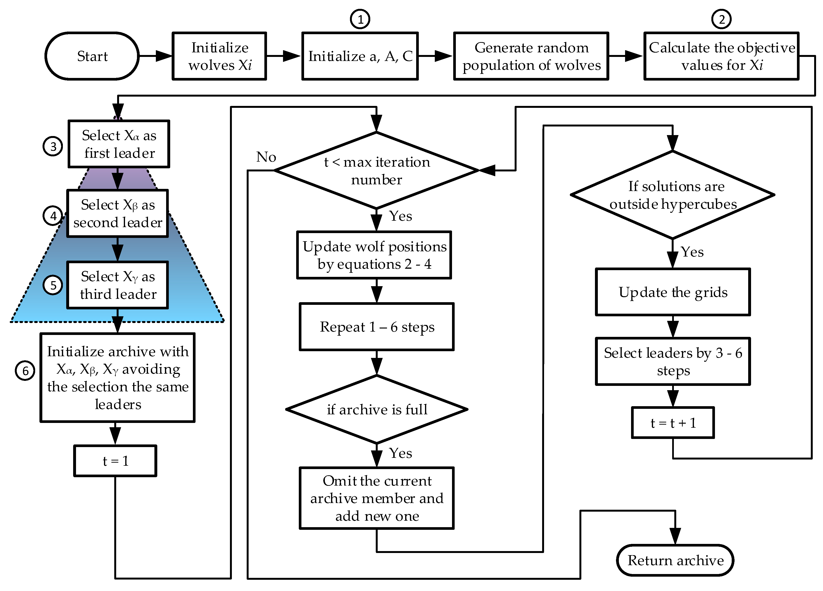
Generally, it can be said that the archive stores the best solutions for each objective function. It saves them not only as alpha, beta, and gamma agents, but also with the segment priorities, which are defined by the number of total solutions. Thus, the global best solution can be chosen among the local ones in the archive. This selection mechanism in MOGWO prevents the picking of the same leaders. In other words, it avoids stagnation in local optimal points. Figure 4 shows the full algorithm of MOGWO.
4. MOGWO Exploration for Multi-Robot System
In this section, we describe the proposed multi-robot exploration based on MOGWO optimization. First, we define the optimization problems in the exploration. As mentioned above, there are two objective functions for which the study tries to find an optimal solution. Then, the second subsection presents the approach for solving the problems using the MOGWO exploration algorithm.
4.1. Mathematical Formulation of MOOPs in the Multi-Robot Exploration
The process of searching uncertainties by a team of robots can be considered a multi-tasking system. Each robot receives the sensor reading data and upgrades the probabilities of the grid occupancy in the map. One robot should have the same task as another robot in the multi-robot system, wherein the task can be any of the following: scanning the environment using sensors, avoiding obstacles and collisions with other robots, seeking to explore new terrain, and increasing the accuracy of the map. It means that together, each single robot should provide good implementation as a multi-robot system satisfying the multi-objective functions for obtaining the best solutions.
In this paper, we formulated the objective functions of the exploration as follows:
Subject to:
where,
The first objective function in Equation (6) tries to maximize the search space by visiting various numbers of cells in the map. In a good scenario, robots should avoid explored cells. The waypoints in MOGWO exploration allow saving the direction to the unexplored part of the map. However, there are some constraints for a successful search. For example, the number of waypoints should not be too small and big. In the case when it is small, robots will stay in one point, because they do not have the tasks to drive next waypoints. If it is bigger than the total number of cells in a map, then a robot will drive around one place longer than it is needed.
After the map is explored, the second objective function tries to improve the map accuracy by reducing the probability values of the grid cells. It means once a sensor beam touches a grid cell, the cell is marked as explored. However, the signal strength projected on the cell is not identical. In the robot position, the probability value has the lowest value. In frontier cells, the values are higher according to the power of a signal.
In the subsection below, the MOGWO exploration algorithm is described extensively.
4.2. The Proposed MOGWO Exploration Algorithm
Equations (6) and (7) define the objectives of the exploration in this study. For such problems, there is no single solution that satisfies all objectives simultaneously at one time. It is not possible to explore new cells (f1) and to revisit explored cells (f2) at the same time. Based on the GWO parameter a in Equation (5), the search process is divided into two parts. When , it searches new waypoints. When , the process switches to revisiting already explored areas to improve the map accuracy. Thus, the approach serves two MOOPs in a single run-time.
Algorithm 1 demonstrates the MOGWO exploration for the multi-robot system. The process begins with the random initialization of waypoints in the search space. Their positions are set only once in the first iteration and will not be upgraded throughout the whole exploration. In line 1, it was noted that the number of waypoints should be higher than because each robot needs at least three of the best solutions for the search.
| Algorithm 1. The pseudocode of the proposed MOGWO exploration 1: Set waypoints randomly in unknown space ( 2: Set the archive is empty 3: Set initial robot position ( 4: Initialize a, A, C 5: while t is not over 6: Update A, C 7: Set the archive is empty 8: for j = 1: nRbt 9: Find current position of 10: Find frontier point (n = 1,…,8) of 11: Insert rays to the map from position 12: Calculate the distances by the objective function () 13: Calculate the probability values by objective function () for 14: if a ≥ 1 15: if is explored 16: Then, to increase cost 17: if else is unexplored 18: Then, cost 19: end if 20: Find minimum costs and save in archive 21: Find of by Equation (2) 22: Find and by Equations (3) and (4) 23: Find 24: end if 25: if a ≤ 1 26: Divide probability cost by distance cost 27: Find maximum costs and save in archive 28: Find 29: end if 30: end for 31: Reduce a 32: show map 33: end while |
The proposed algorithm uses the archive for the same purposes as MOGWO does. It allows the storage of the non-dominated solution, which prevents the repeated selection of the same waypoint by the robots. For each iteration in the loop, the robots upgrade the positions, the GWO parameters, and the positions and probability costs of the frontier cells (lines 9, 10).
Two objective functions are used for all stages (lines 12, 13). The first one calculates the distances between waypoints and robots. The second objective function computes the probability values in the waypoint positions. Thus, the waypoints have distance costs of and probability costs .
Lines 14–24 show the exploration stage for . At first, the algorithm needs to divide the waypoints into explored and unexplored ones due to the probability costs in lines 15–19. Then, it can select the unexplored and according to the distance costs (Figure 5). In lines 21 and 22, it computes the position . However, the robots cannot jump physically to the position, thus, the frontier cell, which is the closest to , is selected for the next robot position.
Lines 25–28 illustrate the exploitation stage for . It divides the probability cost by the distance cost . Afterward, it finds the maximum value of the result in line 26 and saves it in the archive. The next robot position is one of the frontier cells, which is closest to the alpha waypoint.
In line 30, the parameter is reduced from 2 to 0 iteratively. Lastly, the map is upgraded by all robots in the end of iteration.
The implementation results are performed in the next section. The multi-robot exploration by MOGWO algorithm obtained notable results, which can be observed in various conditions by adjusting the numbers of waypoints and iterations.
5. Simulation Results and Analysis
In this section, we implemented the proposed MOGWO exploration and analyzed the obtained results. As alternatives, there are varying parameters for testing the simulation performance such as the number of waypoints and the number of iterations. The parameters are used to test the algorithm performance in several ways. However, some parameters were maintained as constant throughout all the simulation runs (see Table 1).
The major goal, which we seek to attain, is to know how many iterations and how many waypoints are needed for efficient exploration. If the number of iterations is too low, the robots do not have time to explore the entire map physically considering that the size of the step in each iteration is unchanged. The same is true for the number of waypoints. They should be enough for free robot driving in the environment. In the next subsection, the experiments with certain constraints are presented, and the Pareto optimal set is proposed for the selection of the optimal solution of the environment.
5.1. Simulation Results
The analysis of the MOGWO exploration algorithm takes into consideration two aspects of the objective function: how it explores and how it improves the accuracy of the map. The experiment constraints influence the performance of the algorithm. Due to the GWO stochastic parameters, the decision-making process can be different in each simulation run. It leads us to test the algorithm performance several times with the same constraints. Based on the experiment parameters in Table 1, it can be calculated using Equation (8) that the iteration number should not be less than 60 and more than 120. In addition, for the waypoints, the range should be from 60 to 150 for three robots in a certain map size (Equations (9) and (10)). In this study, we selected the parameters as 60, 80, 100, and 120 iterations and 60, 80, 100, and 150 waypoints. Table 2 shows the results of map coverage in percentage, which is computed using the following equation:
In Table 2, it was emphasized that, for example, the maximum map coverage with a certain sequence of decisions and the constraints, 60 iterations by 60 waypoints, is 92.36%. Furthermore, the highest result among all the set of constraints used is 99.47% at the maximum allowable set of constraints.
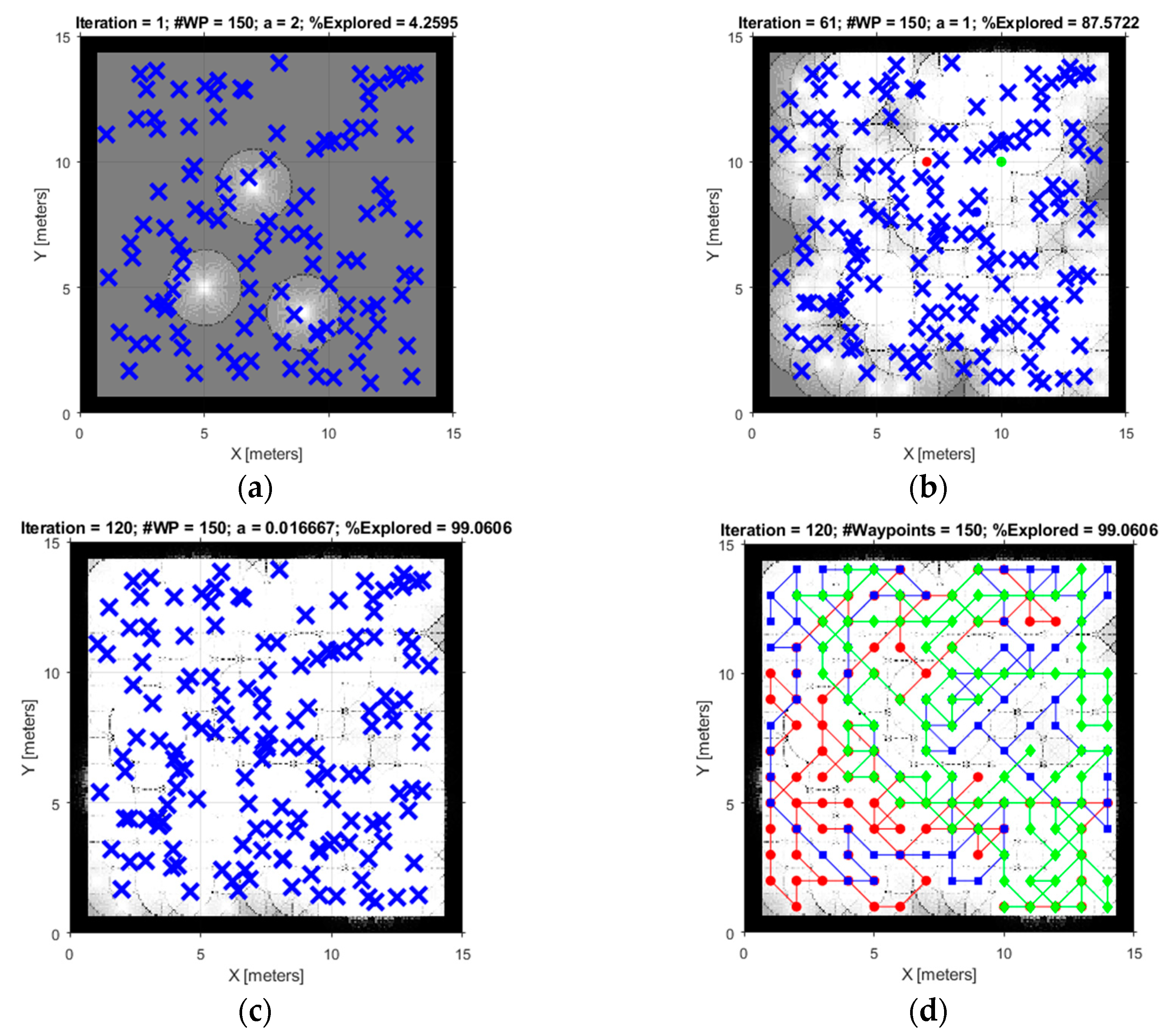
Figure 6 shows one of the simulation-runs with the constraints: 120 iterations and 150 waypoints. In the stage, 87.57% of the environment was explored in half of the total number of iterations (61). For the map in Figure 6b, it can be concluded that the robots touched all the waypoints with the sensor rays. This means that the exploration ability of the algorithm is satisfied in this stage. Figure 6c demonstrates the completed result for the stage with a total of 99.06% map coverage. The trajectories of the robots can be observed through the blue, red, and green colored lines in Figure 6d.
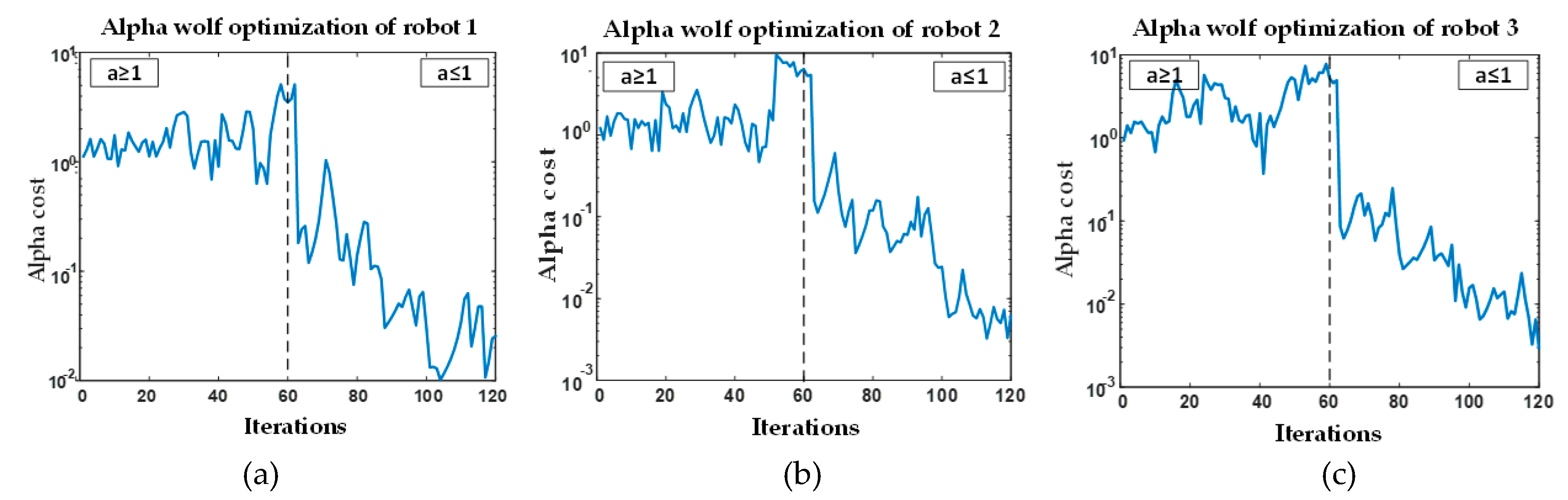
The decision-making process of each robot is presented in Figure 7. The values of alpha solutions in the simulation above (Figure 6) vary for the two stages: exploration and exploitation. It can be seen that when , the trend goes up to maximum values, and when , the simulation tries to achieve the minimum values.
5.2. The Pareto Optimality Analysis for MOGWO Exploration Algorithm
Table 2 shows numerous exploration results, which are categorized by constraints. Considering only the percentage of map coverage, it is obvious that 99.47% is the best performance. However, the exploration with 120 iterations and 150 waypoints as constraints takes the longest time, which means it is not the optimal solution.
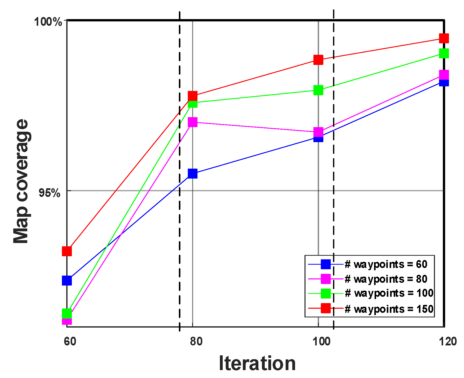
In this study, we take two factors that are important for the exploration: map coverage and time. In Figure 8, we searched for the trade-offs between the minimum number of iterations and the maximum number of map coverage. The plot was made based on the data in Table 2. The results for 120 and 60 iterations, which can be considered too long and too short for exploration, respectively, are extreme solutions. Thus, the solutions belong to the Pareto optimal front, which lies between two lines.
It can be concluded here that the optimal set lies between 80 and 100 iterations with 150 waypoints. In the next subsection, the MOGWO exploration algorithm using 150 waypoints will be compared to two other algorithms using the same environment and map coverage computation using Equation (11).
5.3. Comparison
In this subsection, the proposed MOGWO exploration was compared with the original deterministic CME algorithm [22] and the hybrid stochastic exploration algorithm based on the GWO and CME [8]. The same map and experiment parameters (Table 1) were selected for the two algorithms with 60, 80, 100, and 120 iterations as it was implemented in the MOGWO exploration algorithm in Section 5.1. It should be noted that waypoints were not applied for the other two algorithms used in the comparison.
In the experiment, the CME algorithm was run only once for each iteration class (60, 80, 100, and 120) because it does not generate any random values even when tested multiple times. By its deterministic nature, CME implements differently for every modification in the environment. For instance, the simulation runs were aborted after the 98th iteration during our experiment when one of the robots got stuck next to the wall obstacle. For the purpose of completing the exploration, the initial position of robot 2 or r2 (from Table 1) was changed from (7,9) to (6,5). From these results, we can conclude that the exploration by the deterministic CME algorithm requires fine-tuning the map parameters for successful map coverage.
The hybrid stochastic algorithm is a stochastic approach, which uses the single-based GWO algorithm. During our experiments, the simulation-runs were aborted several times due to the robot’s selection of inappropriate positions among the frontier cells. This situation occurs when the GWO parameters, A and C, oblige a robot to move into the wrong places, such as obstacles or another robot position. Fortunately, in this algorithm, the A and C parameters vary in each simulation-run, which allows us to obtain successful results.
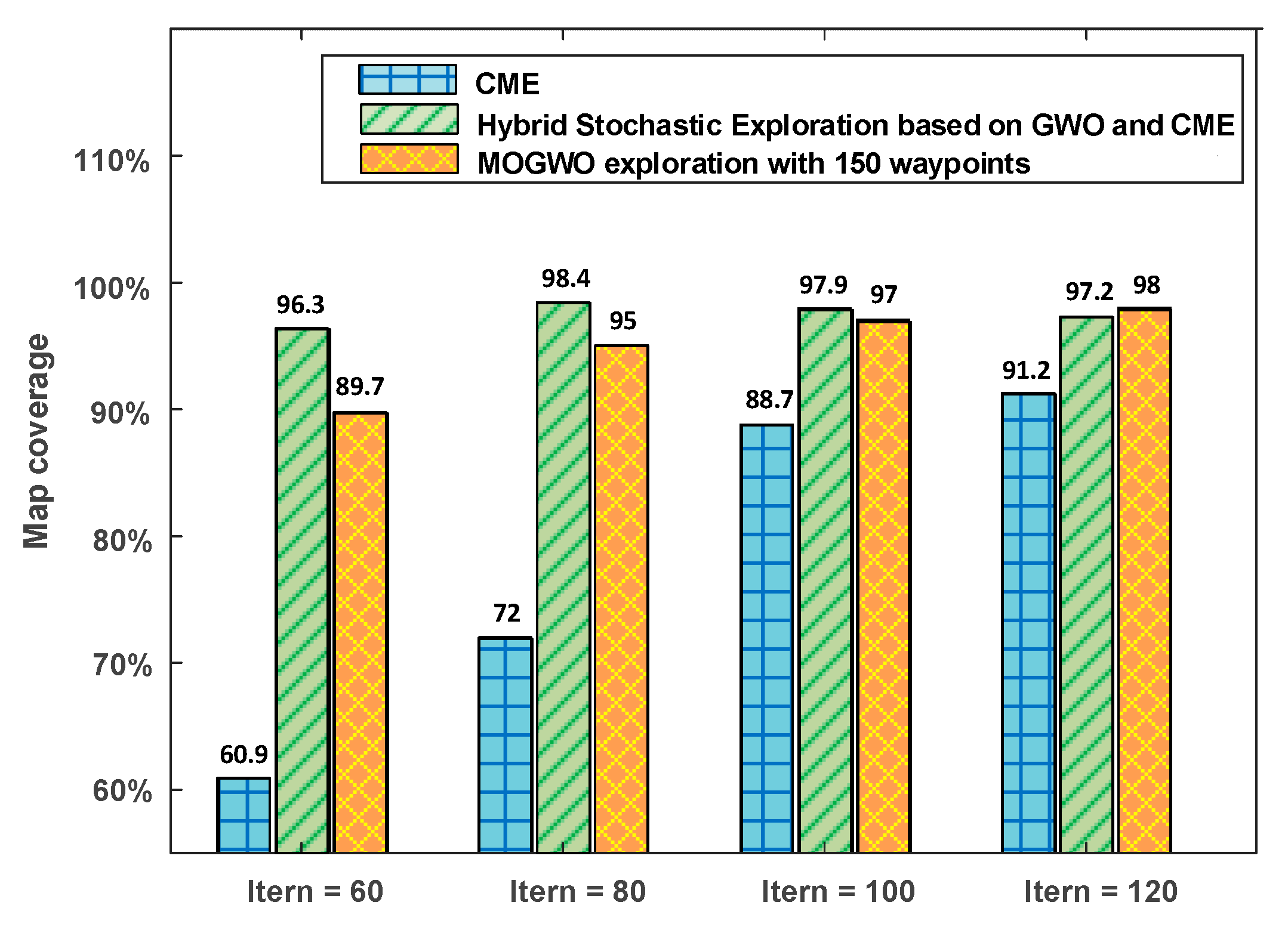
Figure 9 shows the comparison of the results obtained using the original CME, the hybrid stochastic exploration, and the MOGWO exploration with 150 waypoints. It can be seen that the deterministic CME approach has the lowest values of map coverage among all the algorithms. The proposed MOGWO algorithm does not outperform the hybrid stochastic exploration algorithm in iteration classes, 60, 80, and 100. However, it surpasses the original CME in all iteration categories and the hybrid stochastic exploration algorithm in the category of 120 iterations. Additionally, aborted simulation-runs, which are drawbacks of the CME and hybrid stochastic exploration, did not occur in the MOGWO exploration. Thus, the MOGWO exploration proved more efficient and stable compared to the other algorithms studied in this subsection.
6. Conclusions
This paper proposed a new method of solving the multi-robot exploration problem as a multi-objective problem. Two objective functions were formed: to search new terrain and to enhance the map accuracy. The use of the MOGWO algorithm enabled us to obtain high percent values of the map coverage without any aborted simulation-runs. The simulation results successfully demonstrated the capability of the MOGWO algorithm to build complete maps, which were completed within certain constraints: the number of waypoints and the number of iterations. Based on the results, the optimal solution was defined by the Pareto optimal set. Furthermore, the proposed MOGWO exploration algorithm was compared with the deterministic exploration and the hybrid stochastic exploration algorithms. The comparison showed that the proposed MOGWO exploration technique outperforms the deterministic exploration in all set of constraints and the hybrid stochastic exploration algorithm at 120 iterations and 150 waypoints.
Author Contributions
A.K. conceived and designed the algorithm. A.K., S.N. and D.Q. designed and performed the experiments. A.K., S.N. and D.Q. wrote the paper. A.K., D.Q. and S.G.L. formulated the mathematical model. S.G.L. supervised and finalized the manuscript for submission.
Funding
This work was supported by the Basic Science Research Program, through the National Research Foundation of Korea, Ministry of Science, under Grant 2017R1D1A3B04031864.
Conflicts of Interest
The authors declare no conflict of interest.
References
- Limosani, R.; Esposito, R.; Manzi, A.; Teti, G.; Cavallo, F.; Dario, P. Robotic delivery service in combined outdoor–indoor environments: Technical analysis and user evaluation. Robot. Auton. Syst. 2018, 103, 56–67. [Google Scholar] [CrossRef]
- Vidal, E.; Hernández, J.D.; Palomeras, N.; Carreras, M. Online Robotic Exploration for Autonomous Underwater Vehicles in Unstructured Environments. In Proceedings of the IEEE 2018 OCEANS-MTS/IEEE Kobe Techno-Oceans (OTO), Kobe, Japan, 28–31 May 2018; pp. 1–4. [Google Scholar]
- Deb, K. Multi-objective optimization. In Search Methodologies; Springer: Boston, MA, USA, 2014; pp. 403–449. [Google Scholar]
- Amorós, F.; Payá, L.; Marín, J.M.; Reinoso, O. Trajectory estimation and optimization through loop closure detection, using omnidirectional imaging and global-appearance descriptors. Expert Syst. Appl. 2018, 102, 273–290. [Google Scholar] [CrossRef]
- Rizk, Y.; Mariette, A.; Edward, W.T. Cooperative Heterogeneous Multi-Robot Systems: A Survey. ACM Comput. Surv. (CSUR) 2019, 52. [Google Scholar]
- Zhang, Y.; Gong, D.W.; Zhang, J.H. Robot path planning in uncertain environment using multi-objective particle swarm optimization. Neurocomputing 2013, 103, 172–185. [Google Scholar] [CrossRef]
- Pang, B.; Song, Y.; Zhang, C.; Wang, H.; Yang, R. A Swarm Robotic Exploration Strategy Based on an Improved Random Walk Method. J. Robot. 2019, 2019. [Google Scholar] [CrossRef]
- Kamalova, A.; Lee, S.G. Hybrid Stochastic Exploration Using Grey Wolf Optimizer and Coordinated Multi-Robot Exploration Algorithms. IEEE Access 2019, 7, 14246–14255. [Google Scholar]
- Fong, S.; Suash, D.; Ankit, C. A review of metaheuristics in robotics. Comput. Electr. Eng. 2015, 43, 278–291. [Google Scholar] [CrossRef]
- Wadood, A.; Khurshaid, T.; Farkoush, S.G.; Yu, J.; Kim, C.-H.; Rhee, S.-B. Nature-Inspired Whale Optimization Algorithm for Optimal Coordination of Directional Overcurrent Relays in Power Systems. Energies 2019, 12, 2297. [Google Scholar] [CrossRef]
- Kim, C.H.; Khurshaid, T.; Wadood, A.; Farkoush, S.G.; Rhee, S.B. Gray wolf optimizer for the optimal coordination of directional overcurrent relay. J. Electr. Eng. Technol. 2018, 13, 1043–1051. [Google Scholar]
- Wolpert, D.H.; Macready, W.G. No free lunch theorems for optimization. IEEE Trans. Evolut. Comput. 1997, 1, 67–82. [Google Scholar] [CrossRef] [Green Version]
- Kennedy, J. Particle swarm optimization. Encycl. Mach. Learn. 2010, 760–766. [Google Scholar]
- Gen, M.; Lin, L. Genetic Algorithms. Wiley Encyc. Comput. Sci. Eng. 2007, 1–15. [Google Scholar]
- Dorigo, M.; Di Caro, G. Ant colony optimization: A new meta-heuristic. In Proceedings of the 1999 Congress on Evolutionary Computation-CEC99, Washington, DC, USA, 6–9 July 1999. [Google Scholar]
- Seyedali, M.; Lewis, A. Grey wolf optimizer. Adv. Eng. Softw. 2014, 69, 46–61. [Google Scholar]
- Mirjalili, S.; Aljarah, I.; Mafarja, M.; Heidari, A.A.; Faris, H. Grey Wolf Optimizer: Theory, Literature Review, and Application in Computational Fluid Dynamics Problems. In Nature-Inspired Optimizers; Springer: Cham, Switzerland, 2020; pp. 87–105. [Google Scholar]
- Coello, C.A.; Lechuga, M. MOPSO: A proposal for multiple objective particle swarm optimization. In Proceedings of the 2002 Congress on Evolutionary Computation. CEC’02 (Cat. No. 02TH8600), Washington, DC, USA, 12–17 May 2002. [Google Scholar]
- Konak, A.; Coit, D.W.; Smith, A. Multi-objective optimization using genetic algorithms: A tutorial. Reliab. Eng. Syst. Saf. 2006, 91, 992–1007. [Google Scholar] [CrossRef]
- Alaya, I.; Solnon, C.; Khaled, G. Ant colony optimization for multi-objective optimization problems. In Proceedings of the 19th IEEE International Conference on Tools with Artificial Intelligence (ICTAI 2007), Washington, DC, USA, 29–31 October 2007. [Google Scholar]
- Mirjalili, S.; Saremi, S.; Mirjalili, S.M.; Coelho, L.D.S. Multi-objective grey wolf optimizer: A novel algorithm for multi-criterion optimization. Expert Syst. Appl. 2016, 47, 106–119. [Google Scholar] [CrossRef]
- Burgard, W.; Moors, M.; Stachniss, C.; Schneider, F.E. Coordinated multi-robot exploration. IEEE Trans. Robot. 2005, 21, 376–386. [Google Scholar] [CrossRef] [Green Version]
- Thrun, S. A probabilistic on-line mapping algorithm for teams of mobile robots. Int. J. Robot. Res. 2001, 20, 335–363. [Google Scholar] [CrossRef]
- Mirjalili, S.; Dong, J.S.; Lewis, A. Ant Colony Optimizer: Theory, Literature Review, and Application in AUV Path Planning. In Nature-Inspired Optimizers; Springer: Cham, Switzerland, 2020; pp. 7–21. [Google Scholar]
- Kulich, M.; Kubalík, J.; Přeučil, L. An Integrated Approach to Goal Selection in Mobile Robot Exploration. Sensors 2019, 19, 1400. [Google Scholar] [CrossRef]
- Yamauchi, B. A frontier-based approach for autonomous exploration. Cira 1997, 97. [Google Scholar]
- Franchi, A.; Freda, L.; Oriolo, G.; Vendittelli, M. A randomized strategy for cooperative robot exploration. In Proceedings of the 2007 IEEE International Conference on Robotics and Automation, Roma, Italy, 10–14 April 2007. [Google Scholar]
- Franchi, A.; Freda, L.; Oriolo, G.; Vendittelli, M. The sensor-based random graph method for cooperative robot exploration. IEEE/ASME Trans. Mechatron. 2009, 14, 163–175. [Google Scholar] [CrossRef]
- Palacios, A.T.; Sánchez, L.A.; Bedolla Cordero, J.M.E. The random exploration graph for optimal exploration of unknown environments. Int. J. Adv. Robot. Syst. 2017, 14, 1729881416687110. [Google Scholar] [CrossRef]
- Tai, L.; Liu, M. Mobile robots exploration through cnn-based reinforcement learning. Robot. Biomim. 2016, 3, 24. [Google Scholar] [CrossRef] [PubMed] [Green Version]
- Tai, L.; Li, S.; Liu, M. Autonomous exploration of mobile robots through deep neural networks. Int. J. Adv. Robot. Syst. 2017, 14. [Google Scholar] [CrossRef]
- Caley, J.A.; Lawrance, N.R.; Hollinger, G.A. Deep learning of structured environments for robot search. In Proceedings of the 2016 IEEE/RSJ International Conference on Intelligent Robots and Systems (IROS), Daejeon, South Korea, 9–14 October 2016. [Google Scholar]
- Papoutsidakis, M.; Kalovrektis, K.; Drosos, C.; Stamoulis, G. Design of an Autonomous Robotic Vehicle for Area Mapping and Remote Monitoring. Int. J. Comput. Appl. 2017, 167, 36–41. [Google Scholar] [CrossRef]
- Tai, L.; Liu, M. Deep-learning in mobile robotics-from perception to control systems: A survey on why and why not. arXiv 2016, arXiv:1612.07139. [Google Scholar]
- Sharma, S.; Shukla, A.; Tiwari, R. Multi robot area exploration using nature inspired algorithm. Biol. Inspir. Cognit. Archit. 2016, 18, 80–94. [Google Scholar] [CrossRef]
- Wang, D.; Wang, H.; Liu, L. Unknown environment exploration of multi-robot system with the FORDPSO. Swarm Evolut. Comput. 2016, 26, 157–174. [Google Scholar] [CrossRef]
- De Almeida, J.P.L.S.; Nakashima, R.T.; Neves-Jr, F.; de Arruda, L.V.R. Bio-inspired on-line path planner for cooperative exploration of unknown environment by a Multi-Robot System. Robot. Auton. Syst. 2019, 112, 32–48. [Google Scholar] [CrossRef]
- Puig, D.; García, M.A.; Wu, L. A new global optimization strategy for coordinated multi-robot exploration: Development and comparative evaluation. Robot. Auton. Syst. 2011, 59, 635–653. [Google Scholar] [CrossRef]
- Benavides, F.; Ponzoni Carvalho Chanel, C.; Monzón, P.; Grampín, E. An Auto-Adaptive Multi-Objective Strategy for Multi-Robot Exploration of Constrained-Communication Environments. Appl. Sci. 2019, 9, 573. [Google Scholar] [CrossRef]
- Thabit, S.; Mohades, A. Multi-Robot Path Planning Based on Multi-Objective Particle Swarm Optimization. IEEE Access 2019, 7, 2138–2147. [Google Scholar] [CrossRef]
- Chen, X.; Zhang, P.; Du, G.; Li, F. Ant colony optimization based memetic algorithm to solve bi-objective multiple traveling salesmen problem for multi-robot systems. IEEE Access 2018, 6, 21745–21757. [Google Scholar] [CrossRef]
- Hu, P.; Chen, S.; Huang, H.; Zhang, G.; Liu, L. Improved alpha-guided Grey wolf optimizer. IEEE Access 2018, 7, 5421–5437. [Google Scholar] [CrossRef]
- Long, W.; Wu, T.; Cai, S.; Liang, X.; Jiao, J.; Xu, M. A Novel Grey Wolf Optimizer Algorithm with Refraction Learning. IEEE Access 2019, 7, 57805–57819. [Google Scholar] [CrossRef]
- Han, T.; Wang, X.; Liang, Y.; Wei, Z.; Cai, Y. A Novel Grey Wolf Optimizer with Random Walk Strategies for Constrained Engineering Design. In Proceedings of the International Conference on Information Technology and Electrical Engineering, Bandung, Padang, Indonesia, 22–25 October 2018. [Google Scholar]
- Heidari, A.A.; Pahlavani, P. An efficient modified grey wolf optimizer with Lévy flight for optimization tasks. Appl. Soft Comput. 2017, 60, 115–134. [Google Scholar] [CrossRef]
- Gupta, S.; Deep, K. A novel random walk grey wolf optimizer. Swarm Evolut. Comput. 2019, 44, 101–112. [Google Scholar] [CrossRef]
- Fatima, A.; Javaid, N.; Anjum Butt, A.; Sultana, T.; Hussain, W.; Bilal, M.; Ilahi, M. An Enhanced Multi-Objective Gray Wolf Optimization for Virtual Machine Placement in Cloud Data Centers. Electronics 2019, 8, 218. [Google Scholar] [CrossRef]
- Sahoo, A.; Chandra, S. Multi-objective grey wolf optimizer for improved cervix lesion classification. Appl. Soft Comput. 2017, 52, 64–80. [Google Scholar] [CrossRef]
- Wu, C.; Wang, J.; Chen, X.; Du, P.; Yang, W. A novel hybrid system based on multi-objective optimization for wind speed forecasting. Renew. Energy 2020, 146, 149–165. [Google Scholar] [CrossRef]
- Qin, H.; Fan, P.; Tang, H.; Huang, P.; Fang, B.; Pan, S. An effective hybrid discrete grey wolf optimizer for the casting production scheduling problem with multi-objective and multi-constraint. Comput. Ind. Eng. 2019, 128, 458–476. [Google Scholar] [CrossRef]
- Available online: https://www.mathworks.com/help/robotics/ref/robotics.occupancygrid-class.htmlU30T (accessed on 20 July 2019).
- Kumar, N.; Vámossy, Z.; Szabó-Resch, Z.M. Robot path pursuit using probabilistic roadmap. In Proceedings of the 2016 IEEE 17th International Symposium on Computational Intelligence and Informatics (CINTI), Budapest, Hungary, 17–19 November 2016; pp. 139–144. [Google Scholar]
- Available online: https://youtu.be/b_IiUjwM-bQ (accessed on 15 July 2019).
Figure 1.
The proposed Multi-Objective Grey Wolf Optimizer (MOGWO) exploration in two stages: (a) selecting the waypoints in unexplored space with high probability values of occupancy grid map; (b) selecting the closest waypoints in explored space with high probability values proportional to the distance; (c) the next position is one of the frontier points, which is the nearest to the selected waypoint.

Figure 2.
GWO simulation at first iteration: (a) initialization of grey wolf population and searching for the non-dominated agents by the cost sphere function of Equation (1); (b) calculating the divergence of each agent positions to agents in Equation (2); and (c) calculating the next agent position by Equations (3) and (4). The position of agent will change the position in the next iteration to where .

Figure 3.
Two modules of MOGWO: (a) the archive, which consists of three hypercubes, and (b) the leader selection mechanism.
Figure 3.
Two modules of MOGWO: (a) the archive, which consists of three hypercubes, and (b) the leader selection mechanism.

Figure 4.
MOGWO algorithm.

Figure 5.
MOGWO exploration: (a) selection of the closest waypoints among ; (b) the waypoints that are located in the explored space have the lowest probability to be selected by the robot than waypoints in unknown space; (c) the best waypoints for one robots should not be duplicated for another robot.

Figure 6.
The simulation of MOGWO exploration algorithm in (a) iteration 1 with a = 2; (b) iteration 61 with a = 1; (c) the last iteration, 120, with a = 0.016; and (d) the trajectories of three robots.
Figure 6.
The simulation of MOGWO exploration algorithm in (a) iteration 1 with a = 2; (b) iteration 61 with a = 1; (c) the last iteration, 120, with a = 0.016; and (d) the trajectories of three robots.

Figure 7.
Decision-making process of the alpha solutions: (a) robot 1, (b) robot 2, and (c) robot 3.
Figure 7.
Decision-making process of the alpha solutions: (a) robot 1, (b) robot 2, and (c) robot 3.

Figure 8.
Pareto optimal set of the results of the MOGWO exploration algorithm.

Figure 9.
Comparison of three algorithms for the multi-robot exploration. The bars of the hybrid stochastic exploration algorithm based on GWO and coordinated multi-robot exploration (CME) are average values of 30 simulation-runs. The bars of the MOGWO exploration algorithm are average values taken from the row corresponding to 150 waypoints in Table 2.


Table 1.
Experimental parameters.
| Parameters | Value |
|---|---|
| Initial poses | r1 = (5,5), r2 = (7,9), r3 = (4,9) |
| Map size | 15 × 15 |
| Obstacle Width | 0.5 |
| Ray Length | 1.5 |
| Probabilities of occupancy cells | P(robotRx,yR) = 0.0010 |
| P(obstacleRx,yR) = 0.9990 | |
| P(unexploredRx,yR) = 0.5000 | |
| P(unexploredRx,yR) > P(exploredRx,yR) ≥ P(robotRx,yR) |
Table 2.
Simulation results of the MOGWO exploration in several constraints.
| Number of Waypoints | Number of Iterations | |||
|---|---|---|---|---|
| 60 | 80 | 100 | 120 | |
| 60 | 90.17 92.36 82.08 85.55 89.10 85.36 86.58 85.52 90.62 86.79 90.01 82.14 87.78 88.84 88.00 86.03 87.62 89.68 81.42 88.60 92.15 88.48 85.58 84.89 84.16 86.74 86.61 83.59 91.63 84.70 | 92.42 91.16 88.27 90.20 87.91 87.90 90.72 91.70 94.03 91.11 89.21 88.30 93.94 88.85 93.18 90.65 85.15 92.61 94.39 89.23 93.05 90.43 91.99 89.39 93.40 94.95 95.50 93.14 92.40 95.23 | 91.51 85.93 93.54 95.92 96.07 93.47 92.07 92.30 190.33 87.92 95.22 91.70 95.30 88.25 95.76 88.89 93.60 93.46 92.21 90.34 92.77 92.81 91.31 94.86 93.50 88.99 91.83 96.57 94.61 92.46 | 98.21 95.81 95.38 89.61 89.62 89.03 94.26 98.02 96.59 92.89 95.22 93.38 96.33 91.68 94.10 95.99 91.63 93.65 91.60 91.22 97.20 94.28 91.69 95.57 95.84 92.64 95.48 94.63 97.47 97.33 |
| 80 | 90.53 89.00 89.24 90.01 90.24 89.59 88.92 88.62 86.90 87.66 84.95 91.15 89.38 87.89 88.41 88.39 90.47 87.61 82.78 87.21 82.00 82.86 91.21 84.37 89.07 89.44 88.21 89.54 87.64 89.23 | 96.28 93.19 94.32 93.73 94.72 92.70 95.38 96.69 91.98 89.37 90.90 92.56 92.05 93.81 92.11 90.56 97.01 94.86 95.15 94.39 90.49 93.43 91.49 95.56 93.47 90.93 91.19 94.18 92.93 88.49 | 90.16 95.48 94.30 90.94 96.16 86.94 96.42 96.67 94.17 94.85 93.84 95.92 96.61 94.65 94.66 96.51 95.20 92.80 94.89 93.81 96.76 93.81 96.72 95.43 92.19 95.63 91.21 94.38 93.71 92.50 | 96.68 94.28 86.57 97.28 95.38 94.13 98.40 94.95 97.86 94.07 95.16 96.54 96.14 95.16 97.52 94.90 94.76 97.84 96.92 95.63 94.72 92.89 95.91 96.74 94.38 94.67 98.01 97.78 98.45 92.14 |
| 100 | 90.12 87.49 90.16 88.19 87.59 90.10 89.32 92.26 88.19 88.81 87.18 89.89 80.68 87.74 89.14 89.01 89.23 91.39 84.98 88.36 90.95 90.45 87.77 89.86 88.52 86.66 88.18 91.14 86.81 89.48 | 95.34 89.59 93.45 92.88 95.47 95.37 97.58 96.16 91.33 93.93 93.17 95.23 93.77 93.65 95.73 95.55 93.25 94.18 94.71 95.08 92.78 92.91 91.44 86.62 92.31 93.42 92.71 92.62 94.45 94.70 | 95.11 94.45 96.69 97.29 95.81 96.48 93.90 96.97 96.57 96.03 94.61 97.52 92.49 97.32 95.99 96.97 97.49 97.72 97.27 95.42 95.84 94.40 97.11 92.47 94.00 93.77 95.49 97.95 95.40 97.09 | 97.78 97.05 95.14 97.48 95.13 97.11 96.86 98.48 96.17 97.07 96.51 98.17 93.09 96.31 97.09 96.16 98.40 96.43 97.24 96.49 96.67 96.23 95.15 97.56 95.75 95.89 96.38 99.03 94.30 98.03 |
| 150 | 91.15 92.52 92.83 91.41 91.97 86.52 92.14 85.72 92.02 87.60 89.30 91.56 89.73 91.20 84.98 88.67 90.40 88.26 90.52 80.15 88.25 88.63 92.41 93.22 93.22 92.24 88.31 90.85 91.21 86.41 | 96.26 90.48 94.41 95.21 96.27 95.72 95.38 93.91 96.80 95.70 95.75 94.94 95.82 93.62 96.76 91.84 95.58 95.02 96.50 95.98 93.46 96.55 95.52 95.62 95.38 97.78 94.24 93.77 95.94 91.67 | 98.48 98.06 98.41 96.60 98.84 97.24 95.91 95.21 96.83 97.53 97.71 97.34 98.52 95.53 98.54 96.67 97.64 97.26 93.97 96.51 95.28 97.56 96.43 96.52 96.97 95.96 98.27 98.78 96.67 97.27 | 99.06 98.94 98.96 95.48 98.97 97.40 98.21 98.15 97.13 98.33 98.11 97.54 98.31 97.61 96.17 98.19 98.69 98.11 97.26 98.63 94.85 98.13 98.26 98.92 98.49 98.52 97.71 99.47 98.94 98.04 |
© 2019 by the authors. Licensee MDPI, Basel, Switzerland. This article is an open access article distributed under the terms and conditions of the Creative Commons Attribution (CC BY) license (http://creativecommons.org/licenses/by/4.0/).
Share and Cite
MDPI and ACS Style
Kamalova, A.; Navruzov, S.; Qian, D.; Lee, S.G. Multi-Robot Exploration Based on Multi-Objective Grey Wolf Optimizer. Appl. Sci. 2019, 9, 2931. https://doi.org/10.3390/app9142931
AMA Style
Kamalova A, Navruzov S, Qian D, Lee SG. Multi-Robot Exploration Based on Multi-Objective Grey Wolf Optimizer. Applied Sciences. 2019; 9(14):2931. https://doi.org/10.3390/app9142931
Chicago/Turabian StyleKamalova, Albina, Sergey Navruzov, Dianwei Qian, and Suk Gyu Lee. 2019. "Multi-Robot Exploration Based on Multi-Objective Grey Wolf Optimizer" Applied Sciences 9, no. 14: 2931. https://doi.org/10.3390/app9142931
Note that from the first issue of 2016, this journal uses article numbers instead of page numbers. See further details here.