Deep Convolutional Neural Network Model for Automated Diagnosis of Schizophrenia Using EEG Signals

Abstract

A computerized detection system for the diagnosis of Schizophrenia (SZ) using a convolutional neural system is described in this study. Schizophrenia is an anomaly in the brain characterized by behavioral symptoms such as hallucinations and disorganized speech. Electroencephalograms (EEG) indicate brain disorders and are prominently used to study brain diseases. We collected EEG signals from 14 healthy subjects and 14 SZ patients and developed an eleven-layered convolutional neural network (CNN) model to analyze the signals. Conventional machine learning techniques are often laborious and subject to intra-observer variability. Deep learning algorithms that have the ability to automatically extract significant features and classify them are thus employed in this study. Features are extracted automatically at the convolution stage, with the most significant features extracted at the max-pooling stage, and the fully connected layer is utilized to classify the signals. The proposed model generated classification accuracies of 98.07% and 81.26% for non-subject based testing and subject based testing, respectively. The developed model can likely aid clinicians as a diagnostic tool to detect early stages of SZ.

1. Introduction

In the medical field, diseases are often diagnosed by means of laboratory tests, biological markers, or by imaging modalities. However, the diagnosis of diseases encompassing psychiatric disarray is predominantly based on interviews from patients, symptoms presented, and the existence or absence of representative behavioral signs [1]. Schizophrenia (SZ) is a severe, prolonged disorder of the brain that interrupts normal thinking, speech, and the behavioral characteristics of an individual [2]. The National Institute of Mental Health views SZ as a significant contributor to disease burden, with about 2.4 million people in the United States over the age of 18 effected by it [3]. Moreover, the World Health Organization reports that more than 21 million people are affected by SZ worldwide. Schizophrenia is a manifestation of a constellation of symptoms that can include hallucinations, hearing voices that are non-existent, disorganized speech, and functional deterioration, among many others.

Environmental perils such as premature birth, low birth weight, perinatal hypoxia, exposure to an intrauterine virus at an early stage of life, and stressors related to social isolation, migrant status, and urban life at adulthood, subtly hamper brain development, which can lead to the disease [4]. Additionally, since SZ is highly genetic [5], individuals with the genes Neurogranin and Zinc Finger Protein 804A have an increased risk of developing it [6]. Quality of life is then compromised, with most SZ patients being unable to function in workplaces, 20–40% attempting suicide at least once, and between 5–10% successfully committing suicide [7]. Hence, precise and timely prognosis is desired for better treatment and for the recovery of the patient. To date, there is not an established clinical test for SZ, and diagnosis relies on behavioral markers observed by experts. Such assessments are subjective and not very accurate; they fail to capture underlying abnormalities taking place within the brain.

Neuroimaging techniques using multimodal imaging are currently used to detect SZ. Some of these modalities include magnetic resonance imaging, positron emission tomography, functional magnetic resonance imaging, and diffusion tensor magnetic resonance imaging. A combination of the above-mentioned methods may be useful when one imaging modality alone does not explicate the neurological disease of the patient [8]. However, employing a combination of imaging devices may not only be costly for implementation, but also the fusion of images acquired from two different devices may not be of sufficient quality due to motion artifacts [9]. Hence, a more cost-effective method of diagnosing SZ is needed. Electroencephalograms (EEG) are signals which characterize the electrical activity of the human brain recorded from the scalp. It would be very helpful to automatically detect neurological disorders such as epilepsy, depression [10] Parkinson’s disease [11] and Alzheimer’s disease [12,13] by computerized means. Recent studies have analyzed EEG signals for SZ diagnosis [14,15].

Table 1. Parameter details of each layer of the developed CNN model in subject base testing.

Layers	Type of Layer	No. of Neurons (Output Layer)	Kernel Size	Stride
1	Convolution	6248 × 5	3	1
2	Max pooling	3124 × 5	2	2
3	Convolution	3122 × 5	3	1
4	Max pooling	1561 × 5	2	2
5	Convolution	1559 × 5	3	1
6	Average pooling	779 × 5	2	2
7	Convolution	777 × 5	3	1
8	Average pooling	388 × 5	2	2
9	Convolution	386 × 5	3	1
10	Global Average pooling	5	-	-
11	Fully connected	2	-	-

summarizes the published studies of computer-aided detection (CAD) systems using EEG for SZ classification.

Kim et al. [16] extracted EEG recordings with 21 gold cup electrodes placed according to the 10–20 international system, as the horizontal and vertical eye movements of participants were monitored. MATLAB and EGGLAB toolboxes [17] were employed to pre-process the signals, and five frequency bands were selected for analysis. The spectral power of EEG data was computed with fast Fourier transformation, after which the EEG power deviations were studied using the analysis of variance (ANOVA) measure for each of the five frequency bands examined. The diagnostic performance of a test used to distinguish between normal and SZ patients was evaluated with receiver operating curve (ROC) analysis. The delta power was reported to have the highest classification accuracy, at 62.2%. Dvey-Aharon et al. [14] studied the EEG recordings of 50 participants using a 64 electrode array. The electrodes were placed above and beneath the right eye, and laterally with respect to the left and right eyes, to monitor vertical and horizontal eye movements, respectively. The EEG signals were pre-processed, with the raw signals being segmented into relevant intervals, and time-frequency representation was then implemented using the Stockwell transform [18]. Features were extracted from the time-frequency representation, after which certain time frames were discerned based on a set of stimuli between the time-frequency matrix representations of healthy and SZ patients. A high classification accuracy was yielded, with the best five distinct electrodes having a prediction accuracy ranging between 92.0% and 93.9%. The best electrode was found to be F2.

Johannesen et al. [19] acquired EEG recordings from participants using a 64 electrode system, and according to international standards, the patients were tasked with a memory working activity. Participants were required to press one of two response buttons, using either their right or left index finger, to indicate whether a particular letter was presented in the previous set. The signals were analyzed using the Brain Vision Analyser software and segmented via four stages of processing: pre-stimulus baseline, encoding, retention and retrieval. At each of the four stages of processing, time-frequency data (squared wavelet coefficients, binned and averaged according to correct versus incorrect response accuracy) were retrieved for the five frequency bands examined. Statistical analyses were conducted on spectral power measured at the Frontal, Central and Occipital locations. Feature selection was done using the wrapper method [20]. The 1-norm Support Vector Machine (SVM) classifier was utilized to classify correct and incorrect trials in data with the SVM Model 1, yielding a classification accuracy of 84%. The SVM Model 2 was implemented to classify normal versus SZ condition in correct trial data, achieving a classification accuracy of 87%. Santos-Mayo et al. [21] analyzed the EEG-event-related potentials(ERP) signals of participants who were involved in an auditory oddball task. The brain signals were recorded using Brain Vision equipment, in compliance with 10–20 international standards. After acquisition, the signals were pre-processed using EGGLAB, after which 16 time-domain features and four frequency-domain features were extracted per electrode, for each participant. Features were selected via linear discriminant analysis using J5, mutual information feature selection (MIFS), and double input symmetrical relevance. The Multilayer Perceptron (MLP) and SVM classifiers were employed for classification. High classification rates of 93.42% and 92.23% were achieved with the J5 MLP and J5 SVM classifiers, respectively.

Ibanez-Molina et al. [22] acquired EEG recordings from participants while they were at rest and engaged in a naming task. The Neuroscan SynAmps 32-channel amplifier was employed for the data acquirement. EEG signals at the resting phase were acquired prior to the task, while those from the task were extracted after each trial. In the resting phase, the segments were analyzed using a moving window method, after which Lempel–Ziv complexity (LZC) was computed per window. After normalization, the final LZC value was computed by calculating the average of the values obtained from the moving window method. A total of 80 EEG segments of 2 × 10³ ms were evaluated, at task, and then averaged to obtain the final Multiscale LZC value. Higher complexity values were reported in right frontal regions of patients who were at rest. Pang et al. [23] analyzed 2D time and frequency domain connectivity features and 1D intricate network features gauged from EEG signals. These features were then input to the Multi-domain connectome CNN model to obtain feature maps, which aided in the classification process. An accuracy of 93.06% was yielded.

It is notable from Table 1 that most prior studies employed machine learning techniques to diagnose SZ. However, these conventional techniques can be cumbersome, as features require manual extraction and selection prior to SZ classification. Additionally, these methods underperform when large datasets are used. Hence, we have employed a deep convolutional neural network (CNN) model to detect SZ in this study. The novelty of this method lies in the development of an eleven-layered system to distinguish between normal and SZ subjects using EEG signals. Moreover, this model circumvents the typical feature extraction and classification processes, allowing quicker yet more accurate diagnosis.

2. EEG Recording and Preprocessing

EEG signals from 14 patients with paranoid SZ, comprising seven males and seven females, with average ages of 27.9 ± 3.3 and 28.3 ± 4.1 years, respectively, were collected from the Institute of Psychiatry and Neurology in Warsaw, Poland [24]. The exclusion standards involved patients with severe neurological ailments such as Alzheimer’s, early stage SZ, and epilepsy, amongst other considerations, such as pregnancy and existence of a general medical condition. Fourteen healthy subjects within the same age group and gender proportion were recruited for the study from the same institute as well. Each participant provided informed consent to participate in the study upon receiving the study protocol.

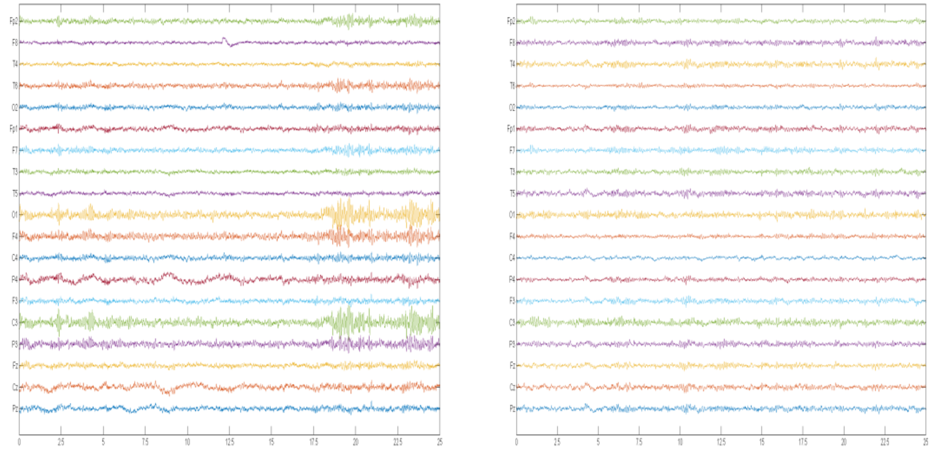
As participants remained in a relaxed state with eyes closed, fifteen minutes of EEG data was collected at a sampling rate of 250 Hz. Data was obtained via the typical International 10–20 System. The electrodes used were Fp1, Fp2, F7, F3, Fz, F4, F8, T3, C3, Cz, C4, T4, T5, P3, Pz, P4, T6, O1, O2. The signals acquired were then divided into segments, in which the signals can be considered to be stationary. Each segment consisted of a 25 s (6250 sample) window length and was normalized with Z-score, before feeding to the one-dimensional deep convolution network for training and testing. A total of 1142 EEG segments were used and each segment consisted of 6250 × 19 sampling points. Normalization was employed to scale the signals to a standard range of values, hence allowing faster convergence by the deep learning model during training. For subject-based testing and non-subject-based testing, 50 epochs and 70 epochs were fed into the network, respectively. An epoch is the dataset that passes forward and backward through a neural network once. An epoch of training for deep learning lasted between 2 to 3 s. For subject-based testing, the validation of the system is executed in three phases: training the data, validation, and testing of data, respectively. During the training phase, k-fold validation is employed, wherein the full data pool is split into fourteen equal parts (subjects). Of these subjects, twelve were used for training, one subject for validation, and one subject for testing, respectively. This process was repeated fourteen times so that all of the fourteen subjects were subjected to the training, validation, and testing phases. In non-subject based testing, the system is validated through the training and testing phases. During the training phase, ten-fold validation is employed, whereby the entire data is split into ten uniform parts. Of these, nine are used for training the model and the remaining one part is used to test. This process is reiterated such that each of the ten portions is involved in both the training and testing phases. Thereafter, 20% of the cross-validation training data is set aside for validation of the model. Figure 1 illustrates an example of EEG recordings from normal and SZ patients.

3. Deep Learning

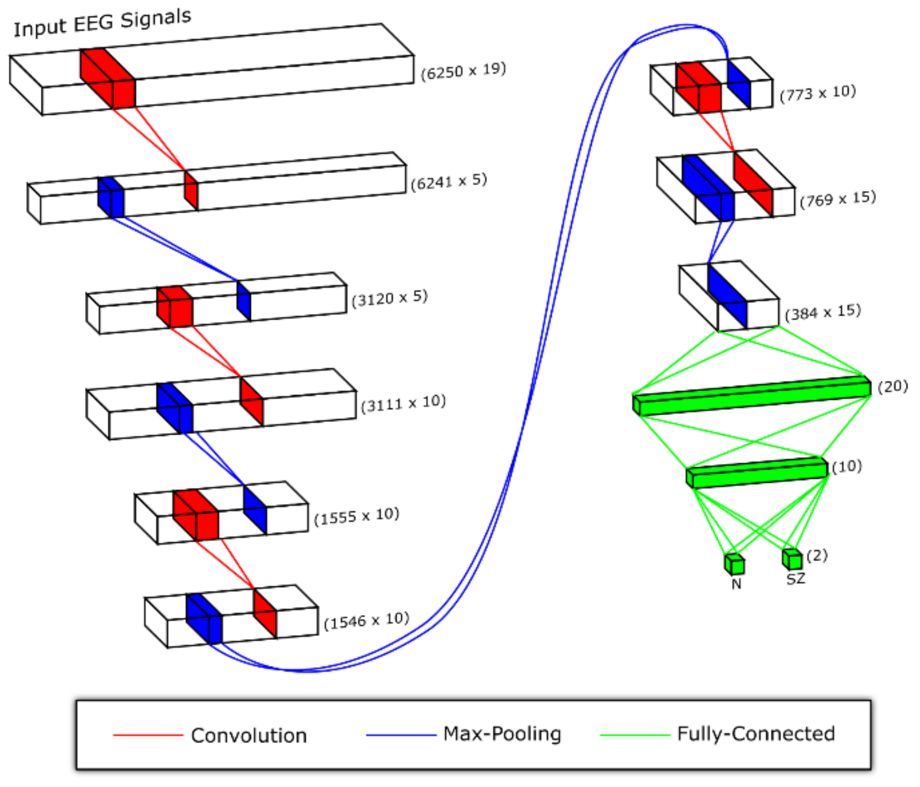
Since EEG signals are nonlinear in nature, nonlinear feature extraction techniques are often employed to differentiate between EEG signals of normal versus SZ patients [25]. Machine learning is prevalently used for pattern recognition. However, this state-of-the-art technique exhibits some impediments. It works well for simple recognition tasks [26], but in realistic settings where the features studied display substantial variability, larger training datasets are needed in order to recognize them [27]. Additionally, a model with a sizeable learning capacity enables higher level features to be studied through learning of data from large datasets as compared to the traditional machine learning techniques. Moreover, conventional techniques require features to be extracted manually. In deep learning, both the feature extraction and classification processes are conducted automatically [28,29] unlike the traditional machine learning techniques. Amongst others, CNN is the most prevalent type of deep learning network that has been exploited by researchers to identify abnormal EEG signals [30] and to study these signals to diagnose disorders such as depression [31], seizure [32], attention deficit hyperactivity disorder [33] and autism [34]. In this study, an eleven-layer deep CNN model has been implemented to discern between normal and SZ classes for non-subject based testing and subject based testing, respectively. Figure 2 and Figure 3 illustrate the models used for non-subject based testing and subject based testing, respectively.

3.1. Convolutional Neural Network

The CNN is a complex network which comprises many masked layers and parameters. The three main tiers in the network are the convolution, max pooling, and fully connected layers [35]. The CNN undergoes a training protocol wherein the convolutional layer uses different sized kernels to interpret the input signal. During convolution, features are extracted from input signals, with the feature maps formed thereafter for the next layer [36]. To normalize the training data, the batch normalization layer is then exercised so that it flows between the middle layers. This helps to expedite and boost the learning process. Max pooling shrinks the size of the feature map, as it yields only the highest number in every kernel. The output from the convolutional and pooling layers portray the top features of the input data. The fully-connected layer then categorizes the input data into the various classes based on the training data. Each neuron in the max pooling and fully-connected layers are connected, whereby the output accurately forecasts the outcome of the input signal as normal or not [37,38].

The system generally learns better with increasing depth of the network; however deeper networks may prolong computational time. Yet, in our study, careful consideration was taken in designing a network that merits a more rapid calibration time. The best classification result is yielded from parameters which are calibrated during training.

3.2. Proposed CNN Architecture

Figure 2 and Figure 3 highlight the architectures proposed in this study. Subject-based testing and non-subject based testing involve different approaches. CNN architecture of subject-based testing uses average pooling layer to obtain smoother features and global average pooling layer at the end to provide more generalized predictions, while the non-subject based testing is a classical CNN architecture that consists of convolution, max pooling and fully connected layers. These structural differences help to enable the model to generalize better during the training phase, depending on the partitioned training and testing data. The non-subject based testing model tends to perform well as we may be using the same subject data for training as well as testing. However, when data are separated based on subject, the classification model needs to learn well the generalized features, in order to classify the new subject data correctly. Hence different architectures of CNN were used.

To improve generalization for subject based testing, dropout is applied to layers 4 and 6 during training, with a dropout rate of 0.5 (meaning that there is 0.5 probability that a neuron will be dropped out during training) but in non-subject based testing, dropout is applied to layers 9 and 10 with a dropout rate of 0.5. Table 1 details the layers used. In subject based testing, Adam optimization [39] parameters, with a learning rate of 0.001, are employed with the Leaky Rectifier Linear Unit (LeakyRelu) and their function is used as the activation functions for layers 1, 3, 5, 7, 9 and 11, respectively. Max pooling is employed after convolution to extract the most crucial features. The average pooling layer is applied after max pooling, to better smooth the features. Subsequently, the global average pooling layer is used instead of the dense layer, in order to obtain a more generalized model. Global average pooling has the upper hand over the dense layer as it does not contain any trainable parameters, thus reducing the likelihood of overfitting. All of the factors are fine-tuned based on the training set that provides the optimal training accuracy. The number of filters and kernel size were determined via the brute force technique. Classification was then done with the help of the fully-connected layer.

In non-subject based testing, Adam optimization parameters with a learning rate of 0.0001 are used with LeakyRelu and Softmax functions for layers 1, 3, 5, 7, 9, 10 and 11, respectively. Max pooling is applied after convolution at each stage to extract the most important features.

Table 2. Parameter details of each layer of the developed CNN model in non-subject based testing.

Layers	Type of Layer	No. of Neurons (Output Layer)	Kernel Size	Stride
1	Convolution	6241 × 5	10	1
2	Max pooling	3120 × 5	2	2
3	Convolution	3111 × 10	10	1
4	Max pooling	1555 × 10	2	2
5	Convolution	1546 × 10	10	1
6	Max pooling	773 × 10	2	2
7	Convolution	769 × 15	5	1
8	Max pooling	384 × 15	2	2
9	Fully connected	20	-	-
10	Fully connected	10	-	-
11	Fully connected	2	-	-

highlights the details of all layers used. The model with the best validation accuracy was considered during training and testing. Classification was then done with the help of the fully-connected layer.

3.3. Results

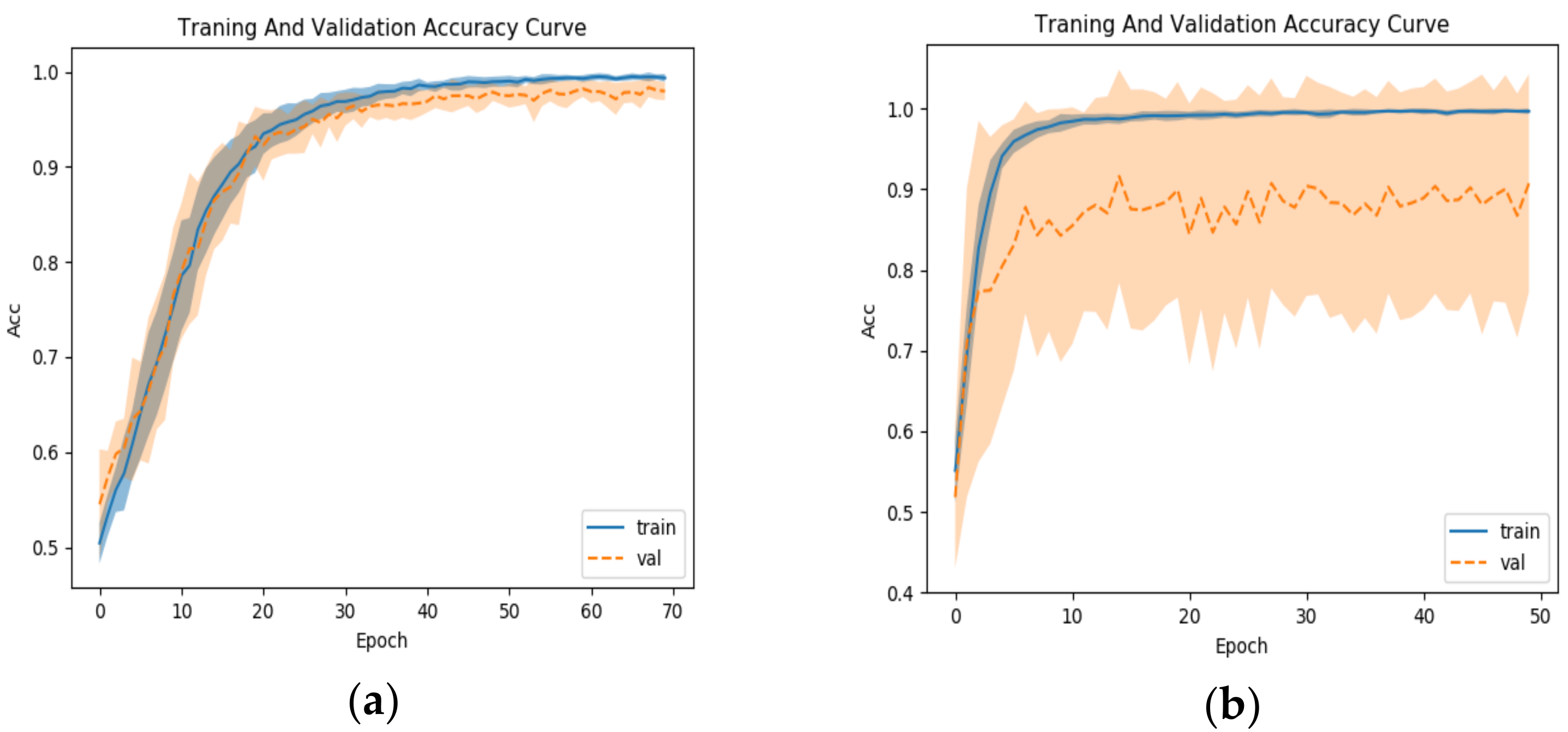
The CNN network employed in this study was designed using Two Intel Xeon 2.40 GHz (E5620) processors with 24 GB RAM and the Intel(R) Xeon(R) CPU E5-2650 v4 2.20GHz (2 processors), 384 GB RAM and NVIDIA Quadro K4200. Accuracy, sensitivity, positive predictive value, and specificity were utilized as the assessment parameters.

Table 3. Classification result per fold for subject based testing.

Fold	Accuracy (%)	PPV (%)	Sensitivity (%)	Specificity (%)
1	87.14	100.00	72.73	100.00
2	100.00	100.00	100.00	100.00
3	51.35	100.00	5.26	100.00
4	100.00	100.00	100.00	100.00
5	94.44	100.00	88.57	100.00
6	65.15	100.00	20.69	100.00
7	69.66	66.67	98.11	27.78
8	77.78	95.45	58.33	97.22
9	55.42	56.10	97.87	0.00
10	55.13	0.00	0.00	97.73
11	98.89	100.00	98.15	100.00
12	72.15	100.00	48.84	100.00
13	100.00	100.00	100.00	100.00
14	96.67	95.56	100.00	88.24

and

Table 4. Classification result per fold for non-subject based testing.

Fold	Accuracy (%)	PPV (%)	Sensitivity (%)	Specificity (%)
1	96.52	98.36	95.24	98.08
2	99.13	100.00	98.41	100.00
3	99.13	100.00	98.41	100.00
4	96.52	95.38	98.41	94.23
5	100.00	100.00	100.00	100.00
6	98.26	100.00	96.83	100.00
7	94.69	95.16	95.16	94.12
8	98.23	98.39	98.39	98.04
9	99.12	100.00	98.39	100.00
10	99.12	100.00	98.39	100.00

show the classification result per fold for subject based testing and non-subject based testing, respectively. The best diagnostic performance for the subject based testing is achieved with a learning rate of 0.001 while that of the non-subject based testing it is 0.0001. Figure 4a,b indicate the performance of the network with dropout layers. It is notable that the accurateness of the training set does not deviate substantially from that of the validation set in Figure 4a, when dropout is added to layers 9 and 10 during training for non-subject base testing. However, in Figure 4b, the accuracy of the training set is far better than that of the validation set, when dropout is added to layers 4 and 6 during training for the subject base testing. The proposed architecture generated high accuracy, sensitivity, specificity, and positive predictive values of 98.07%, 97.32%, 98.17%, 98.45% and 81.26%, 75.42%, 87.59%, 87.59%, for the non-subject based testing and subject based testing, respectively. It is apparent that non-subject based testing using 10-fold yields results of higher accuracy compared to subject based testing using 14-fold. Figure 5 shows the confusion matrix result. Based on Figure 5a, it is evident that 13.18% of healthy subjects are miscategorized as SZ patients and 23.32% of healthy subjects are incorrectly classified as SZ patients. In Figure 5b, 1.56% of healthy subjects are miscategorized as SZ patients and of 2.24% healthy subjects are wrongly classified as SZ patients.

4. Discussion

4.1. Comparison with Related Work

Among related work, Kim et al. [16] exploited feature extraction methods on the different brain waves and obtained an accuracy of 62.2% on the delta frequency band. Dvey-Aharon et al. [14] also explored feature extraction methods on beta brain waves and obtained an accuracy between 91.5% and 93.9%. Johannesen et al. [19] analyzed five brain waves using a software program and employed statistical analysis and feature selection. Two SVM models were then implemented for classification, with accuracies of 84% and 87% yielded for models 1 and 2, respectively. Santos-Mayo et al. [21] extracted features by employing feature extraction methods and selected features via linear discriminant analyses. Classification accuracies of 93.42% and 92.23% were achieved with the J5 MLP and J5 SVM classifiers, respectively. Ibanez-Molina et al. [21] used the moving window method to compute Multiscale LZC to analyze brain signals. The study revealed that higher complexity values were present in right frontal regions of patients who were at rest. Pang et al. [23] employed the Multi-domain connectome CNN model to classify extracted features with an accuracy of 93.06%. It can be noted from

Table 5. Summarized studies of computer-aided detection (CAD) systems using EEG for SZ classification.

Authors	Number of Features	Techniques	Number of Participants	Classification Results
Kim et al. [16], 2015	-	▪ Spectral power of EEG computed with Fast Fourier Transformation using MATLAB (covariates) ▪ Delta, Theta, Alpha 1 and 2, Beta frequency bands analysed. ▪ Analysis of variance (ANOVA), ROC analysis. ▪ QEEG parameters	Normal: 90 healthy subjects SZ: 90 patients	Best classification Acc: Delta frequency band, 62.2%.
Dvey-Aharon et al. [14], 2015	-	▪ Time-frequency transformation ▪ Feature-Optimisation ▪ Beta2 band frequencies ▪ Leave one out cross validation	Normal: 25 healthy subjects SZ: 25 patients	Best electrodes that differentiate the 2 classes: F2, FC3 Classification Acc: between 91.5% and 93.9%.
Johannesen et al. [19], 2016	60 features per participant	▪ Theta 1 and 2, alpha, beta and gamma frequency bands analysed during a working memory task. ▪ Brain Vision Analyser software to analyse signals ▪ Support vector machine (SVM) to build EEG classifiers ▪ Regression-based analyses used to validate SVM models.	Normal: 12 healthy subjects SZ: 40 patients	Model 1: Achieved 84% accuracy in classifying SZ and healthy individuals. Model 2: Achieved 87% classification accuracy in discriminating healthy and SZ patients.
Santos-Mayo et al. [21], 2017	20 per subject	▪ P3b brain signals ▪ Time, frequency domain features ▪ Channel grouping ▪ J5, mutual information feature selection (MIFS) or DISR feature selection algorithms ▪ SVM, Multilayer perceptron (MLP) classifiers	Normal: 31 healthy subjectsSZ: 16 patients	Using 15 Hz-J5-MLP Acc: 93.42 %Sen: 87.27% Spe: 96.73% Using 35 Hz-J5-SVM Acc: 92.23% Sen: 88.38% Spe: 94.99%
Ibanez-Molina et al. [22], 2018	-	▪ EEG signals analysed at rest and during picture naming. ▪ Neuroscan SynAmps 32-channel amplifier. ▪ Lempel–Ziv complexity (LZC), Multiscale LZC. ▪ Feature selection using J5, MIFS, DISR.	Normal: 17 healthy subjects SZ: 18 patients	Healthy subjects had lesser errors made compared to patients. Higher complexity values were found inpatients, in right frontal regions at rest but no differences were found between the two groups during the naming activity. Higher complexity values were observed in SZ patients at rest, compared to at task.
Pang et al. [23], 2019	-	▪ Multi-domain connectome CNN model ▪ 2D time and frequency domain connectivity features gauged from EEG signals ▪ 1D intricate network features gauged from EEG signals. ▪ Feature maps obtained for classification via features fed into CNN.	Normal: 39 healthy subjects SZ: 45 patients	Acc: 93.06%
Present work	-	▪ 11-layered deep CNN model ▪ Subject base testing using 14-fold ▪ Non-subject base testing using 10-fold	Normal: 14 healthy subjects SZ: 14patients	Non-subject base testing: Acc: 98.07% Sen: 97.32% Spe: 98.17% Ppv: 98.45% Subject base testing: Acc: 81.26% Sen: 75.42% Spe: 87.59% Ppv: 87.59%

Acc—accuracy, Sen—sensitivity, Spe—specificity, Ppv—positive predictive value.

that the current state-of-the-art techniques can be employed to classify SZ accurately. Comparing the different techniques discussed, it is evident that the highest accuracy is yielded for the classification of SZ using the CNN deep learning algorithm. In non-subject based testing, the segments used for training and testing are split randomly, wherein the subjects are not truly separated, resulting in higher accuracy, as compared to subject based testing, wherein the segments are not randomly split. Hence, using 10-fold validation [40,41] for non-subject based testing generated more accurate results as compared to 14-fold validation for subject based testing. The model developed in our study and described herein could potentially also be used to diagnose other neurological disorders such as Alzheimer′s, Parkinson’s disease, and epilepsy. Apart from the CNN model, other deep learning methods such as long short-term memory (LSTM) and autoencoders could also be explored in the diagnosis of SZ.

4.2. Merits and Drawbacks of the New Paradigm

The main advantages of the proposed system include:

(1)

An eleven-layered CNN model has been developed to accurately assess SZ patients versus controls.

(2)

The CNN model does the extraction, selection, and classification processes automatically.

(3)

The model is validated with the highly graded 10-fold cross validation technique.

(4)

High accuracy with a small data size is an attestation to the robustness of the system.

Despite its high classification accuracy, the proposed system does exhibit some limitations. The main disadvantages of the proposed system are:

(1)

The CNN model was developed using a small data pool of 14 healthy subjects and 14 SZ patients.

(2)

Compared to the traditional machine learning techniques, CNN is costly to compute.

5. Future Work

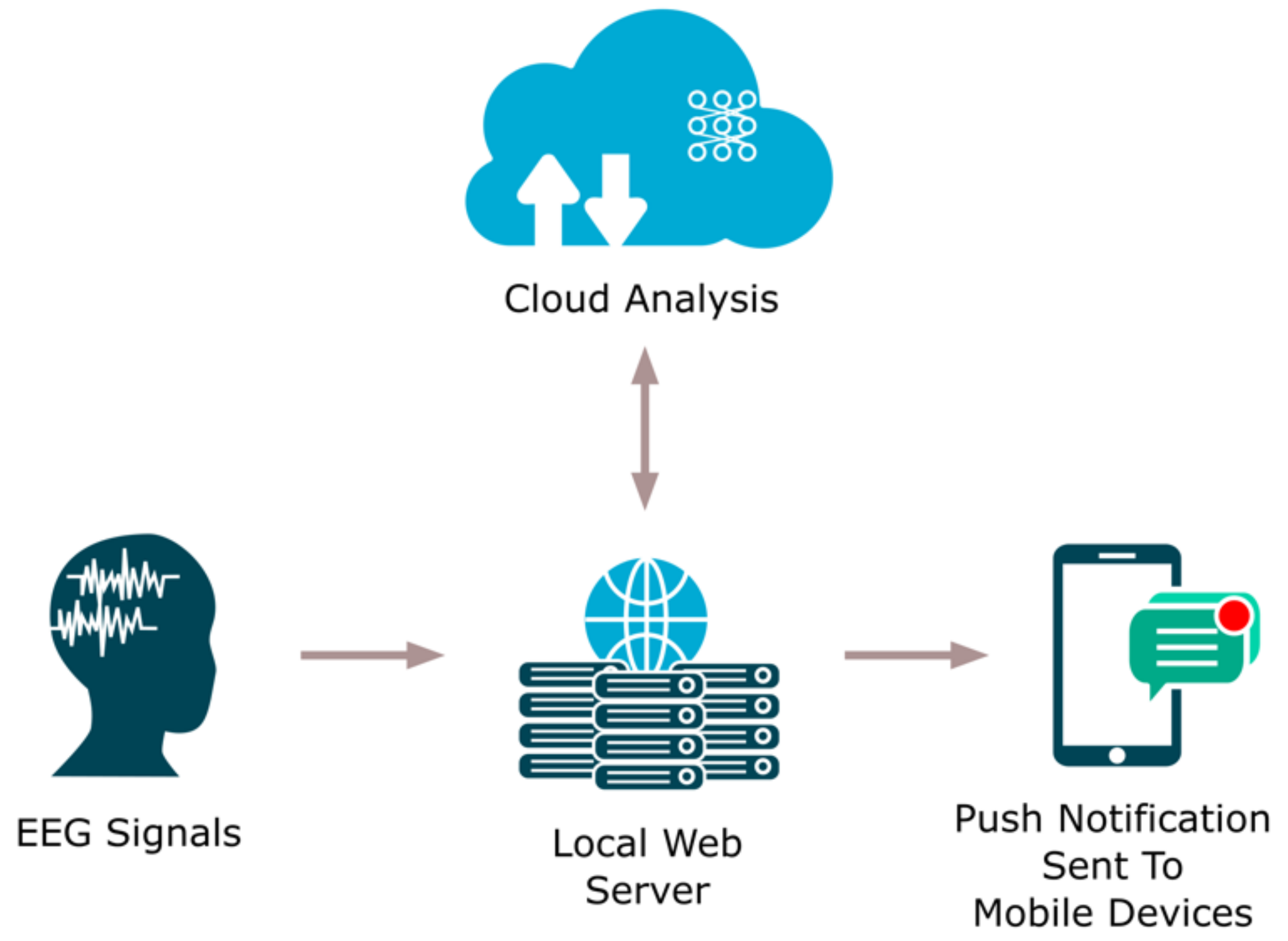
To improve the efficacy of our CAD system, we propose adding a web-based detection component to the existing model. Figure 6 highlights how the added component would work. This method taps the Internet for SZ patient diagnostics. The EEG signals gathered from patients would be saved in the server within the clinic or hospital and sent to cloud, wherein the developed CNN model is positioned. The diagnostic result is then ported to the clinic or hospital via the cloud. Additionally, this technique has an edge over others, as the diagnostic result can also be sent directly to the patient via a push notification ported to mobile devices. With the implementation of this system, the task of healthcare professionals can be made easier.

6. Conclusions

An eleven-layered CNN model was proposed to detect SZ using EEG signals. High classification accuracies of 98.07% and 81.26% were obtained for non-subject based testing and subject based testing, respectively, despite the small data pool. With the proposed technique, exhaustive screening of SZ patients to alert for behavioral markers of the disease is not required, as the model is satisfactory in automatically assisting with the diagnosis. This robust system is foreseen to be a windfall to clinicians as a diagnostic tool, aiding them in SZ assessment. In the near future, we intend to use a larger dataset to test our model, and also plan to combine the web-based cloud method to identify the early stages of SZ.

References

- Savio, A.; Charpentier, J.; Termenon, M.; Shinn, A.K.; Graña, M. Neural classifiers for schizophrenia diagnostic support on diffusion imaging data. Neural Netw. World 2010, 20, 935–949. [Google Scholar]
- Chatterjee, I.; Agarwal, M.; Rana, B.; Lakhyani, N.; Kumar, N. Bi-objective approach for computer-aided diagnosis of schizophrenia patients using fMRI data. Multimed. Tools Appl. 2018, 77, 26991–27015. [Google Scholar] [CrossRef]
- Wing, J.K. Recent advances in understanding schizophrenia. Disabil. Rehabil. 1979, 1, 79–82. [Google Scholar] [CrossRef]
- Boydell, J.; van Os, J.; McKenzie, K.; Murray, R.M. The association of inequality with the incidence of schizophrenia-An ecological study. Soc. Psychiatry Psychiatr. Epidemiol. 2004, 39, 597–599. [Google Scholar] [CrossRef] [PubMed]
- Clark, A. Gene expression as a complex trait. Comp. Biochem. Physiol. Part A Mol. Integr. Physiol. 2003, 124, 2003. [Google Scholar] [CrossRef]
- Williams, H.J.; Norton, N.; Dwyer, S.; Moskvina, V.; Nikolov, I.; Carroll, L.; Georgieva, L.; Williams, N.M.; Morris, D.W.; Quinn, E.M.; et al. Fine mapping of ZNF804A and genome-wide significant evidence for its involvement in schizophrenia and bipolar disorder. Mol. Psychiatry 2010, 16, 429. [Google Scholar] [CrossRef] [PubMed]
- Tibbetts, P.E. Principles of cognitive neuroscience. Second Edition /Principles of neuroscience. Fifth Edition. Q. Rev. Biol. 2013, 88, 139–140. [Google Scholar] [CrossRef]
- Boeve, B.F.; Lowe, V.J.; Weigand, S.D.; Wiste, H.J.; Senjem, M.L.; Knopman, D.S.; Shiung, M.M.; Gunter, J.L.; Boeve, B.F.; Kemp, B.J.; et al. Serial PIB and MRI in normal, mild cognitive impairment and Alzheimer’s disease: Implications for sequence of pathological events in Alzheimer’s disease. Brain 2009, 132, 1355–1365. [Google Scholar]
- Wehrl, H.F.; Amend, M.; Thielcke, A. Multimodal Imaging and Image Fusion. In Small Animal Imaging: Basics and Practical Guide; Kiessling, F., Pichler, J.B., Hauff, P., Eds.; Cham Springer International Publishing: Berlin/Heidelberg, Germany, 2017; pp. 491–507. [Google Scholar]
- Acharya, U.R.; Sudarshan, V.K.; Adeli, H.; Santhosh, J.; Koh, J.E.; Puthankatti, S.D.; Adeli, A. A novel depression diagnosis index using nonlinear features in EEG signals. Eur. Neurol. 2015, 74, 79–83. [Google Scholar] [CrossRef]
- Oh, S.L.; Hagiwara, Y.; Raghavendra, U.; Yuvaraj, R.; Arunkumar, N.; Murugappan, M.; Acharya, U.R. A deep learning approach for Parkinson’s disease diagnosis from EEG signals. Neural Comput. Appl. 2018. [Google Scholar] [CrossRef]
- Hampel, H.; Frank, R.; Broich, K.; Teipel, S.J.; Katz, R.G.; Hardy, J.; Herholz, K.; Bokde, A.L.; Jessen, F.; Hoessler, Y.C.; et al. Biomarkers for Alzheimer’s disease: Academic, industry and regulatory perspectives. Nat. Rev. Drug Discov. 2010, 9, 560–574. [Google Scholar] [CrossRef]
- Gandal, M.J.; Edgar, J.C.; Klook, K.; Siegel, S.J. Gamma synchrony: Towards a translational biomarker for the treatment-resistant symptoms of schizophrenia. Neuropharmacology 2012, 62, 1504–1518. [Google Scholar] [CrossRef] [Green Version]
- Dvey-Aharon, Z.; Fogelson, N.; Peled, A.; Intrator, N. Schizophrenia detection and classification by advanced analysis of EEG recordings using a single electrode approach. PLoS ONE 2015, 10, e0123033. [Google Scholar] [CrossRef]
- Boostani, R.; Sadatnezhad, K.; Sabeti, M. An efficient classifier to diagnose of schizophrenia based on the EEG signals. Expert Syst. Appl. 2009, 36, 6492–6499. [Google Scholar] [CrossRef]
- Kim, J.W.; Lee, Y.S.; Han, D.H.; Min, K.J.; Lee, J.; Lee, K. Diagnostic utility of quantitative EEG in un-medicated schizophrenia. Neurosci. Lett. 2015, 589, 126–131. [Google Scholar] [CrossRef]
- Delorme, A.; Makeig, S. EEGLAB: an open source toolbox for analysis of single-trial EEG dynamics including independent component analysis. J. Neurosci. Methods 2004, 134, 9–21. [Google Scholar] [CrossRef] [Green Version]
- Stockwell, R.G.; Mansinha, L.; Lowe, R.P. Localization of the complex spectrum: the S transform. IEEE Trans. Signal Process 1996, 44, 998. [Google Scholar] [CrossRef]
- Chen, C.M.A.; Jiang, R.; Kenney, J.G.; Bi, J.; Johannesen, J.K. Machine learning identification of EEG features predicting working memory performance in schizophrenia and healthy adults. Neuropsychiatr. Electrophysiol. 2016, 2, 1–21. [Google Scholar]
- Guyon, I. An Introduction to Variable and Feature Selection. J. Mach. Learn. Res. 2003, 3, 1157–1182. [Google Scholar]
- Santos-Mayo, L.; San-José-Revuelta, L.M.; Arribas, J.I. A Computer-Aided Diagnosis System With EEG Based on the P3b Wave During an Auditory Odd-Ball Task in Schizophrenia. IEEE Trans. Biomed. Eng. 2017, 64, 395–407. [Google Scholar] [CrossRef]
- Ibáñez-Molina, A.J.; Lozano, V.; Soriano, M.F.; Aznarte, J.I.; Gómez-Ariza, C.J.; Bajo, M.T. EEG multiscale complexity in schizophrenia during picture naming. Front. Physiol. 2018, 9, 1–12. [Google Scholar] [CrossRef]
- Phang, C.R.; Ting, C.M.; Noman, F.; Ombao, H. Classification of EEG-Based Brain Connectivity Networks in Schizophrenia Using a Multi-Domain Connectome Convolutional Neural Network. arXiv 2019, arXiv:1903.08858. [Google Scholar]
- Olejarczyk, E.; Jernajczyk, W. Graph-based analysis of brain connectivity in schizophrenia. PLoS ONE 2017, 12, e0188629. [Google Scholar] [CrossRef]
- Hornero, R.; Abasolo, D.; Jimeno, N.; Sanchez, C.I.; Poza, J.; Aboy, M. Variability; regularity; complexity of time series generated by schizophrenic patients and control subjects. IEEE Trans. Biomed. Eng. 2006, 53, 210–218. [Google Scholar] [CrossRef]
- LeCun, Y.; Huang, F.J.; Bottou, L. Learning methods for generic object recognition with invariance to pose and lighting. In Proceedings of the 2004 IEEE Computer Society Conference on Computer Vision and Pattern Recognition; CVPR 2004, Washington, DC, USA, 27 June–2 July 2004; Volume 2, pp. 97–104. [Google Scholar]
- Krizhevsky, A.; Sutskever, I.; Hinton, G.E. ImageNet Classification with Deep Convolutional Neural Networks. In Proceedings of the 25th International Conference on Neural Information Processing Systems, Lake Tahoe, Nevada, 3–6 December 2012. [Google Scholar]
- Acharya, U.R.; Fujita, H.; Lih, O.S.; Hagiwara, Y.; Tan, J.H.; Adam, M. Automated detection of arrhythmias using different intervals of tachycardia ECG segments with convolutional neural network. Inf. Sci. 2017, 405, 81–90. [Google Scholar] [CrossRef]
- Acharya, U.R.; Fujita, H.; Lih, O.S.; Adam, M.; Tan, J.H.; Chua, C.K. Automated detection of coronary artery disease using different durations of ECG segments with convolutional neural network. Knowl. Based Syst. 2017, 132, 62–71. [Google Scholar] [CrossRef]
- Yıldırım, Ö.; Baloglu, U.B.; Acharya, U.R. A deep convolutional neural network model for automated identification of abnormal EEG signals. Neural Comput. Appl. 2018, 1–12. [Google Scholar] [CrossRef]
- Acharya, U.R.; Oh, S.L.; Hagiwara, Y.; Tan, J.H.; Adeli, H.; Subha, D.P. Automated EEG-based screening of depression using deep convolutional neural network. Comput. Methods Programs Biomed. 2018, 161, 103–113. [Google Scholar] [CrossRef]
- Acharya, U.R.; Oh, S.L.; Hagiwara, Y.; Tan, J.H.; Adeli, H. Deep convolutional neural network for the automated detection and diagnosis of seizure using EEG signals. Comput. Biol. Med. 2018, 100, 270–278. [Google Scholar] [CrossRef]
- Sridhar, C.; Bhat, S.; Acharya, U.R.; Adeli, H.; Bairy, G.M. Diagnosis of attention deficit hyperactivity disorder using imaging and signal processing techniques. Comput. Biol. Med. 2017, 88, 93–99. [Google Scholar] [CrossRef]
- Bhat, S.; Acharya, U.R.; Adeli, H.; Bairy, G.M.; Adeli, A. Autism: cause factors, early diagnosis and therapies. Rev. Neurosci. 2014, 25, 841–850. [Google Scholar] [CrossRef]
- Faust, O.; Hagiwara, Y.; Hong, T.J.; Lih, O.S.; Acharya, U.R. Deep learning for healthcare applications based on physiological signals: A review. Comput. Methods Programs Biomed. 2018, 161, 1–13. [Google Scholar] [CrossRef]
- Lecun, Y.; Bengio, Y.; Hinton, G. Deep learning. Nature 2015, 521, 436–444. [Google Scholar] [CrossRef]
- Scherer, D.; Müller, A.; Behnke, S. Evaluation of pooling operations in convolutional architectures for object recognition. Lect. Notes Comput. Sci. 2010, 6354 LNCS Pt 3, 92–101. [Google Scholar]
- Serre, T.; Wolf, L.; Poggio, T. Object recognition with features inspired by visual cortex. In Proceedings of the 2005 IEEE Computer Society Conference on Computer Vision and Pattern Recognition; CVPR 2005, San Diego, CA, USA, USA, 20–25 June 2005; pp. 994–1000. [Google Scholar]
- Kingma, D.P.; Ba, J.L. Adam: A Method for Stochastic Optimisation. arXiv 2014, arXiv:1412.6980. [Google Scholar]
- Seymour, G. Predictive Inference, Monographs on Statistics and Applied Probability; Routledge: Abingdon, UK, 1993. [Google Scholar]
- Schaffer, C. Technical Note: Selecting a Classification Method by Cross-Validation. Mach. Learn. 1993, 13, 135–143. [Google Scholar] [CrossRef]
Figure 1.
Illustration of normal (left) and Schizophrenia (SZ) (right) Electroencephalograms (EEG) recordings. (X axis: seconds, Y axis: channels).
Figure 2.
The proposed convolutional neural network (CNN) model for non-subject based testing.
Figure 3.
The proposed CNN model for subject based testing.
Figure 4.
Accuracy versus different epoch plot for (a) non-subject based testing and (b) subject based testing.
Figure 5.
Confusion matrix of (a) non-subject based testing and (b) subject based testing.
Figure 6.
Illustration of the proposed cloud model.