Concrete Cracks Detection Based on FCN with Dilated Convolution


1
Hunan Provincial Key Laboratory of Intelligent Processing of Big Data on Transportation, School of Computer and Communication Engineering, Changsha University of Science and Technology, Changsha 410114, China
2
School of Information Science and Engineering, Fujian University of Technology, Fuzhou 350118, China
3
School of Civil Engineering, Changsha University of Science and Technology, Changsha 410114, China
4
Rattanakosin International College of Creative Entrepreneurship, Rajamangala University of Technology Rattanakosin, Nakhon Pathom 73170, Thailand
*
Author to whom correspondence should be addressed.
Appl. Sci. 2019, 9(13), 2686; https://doi.org/10.3390/app9132686
Submission received: 4 June 2019
/
Revised: 27 June 2019
/
Accepted: 29 June 2019
/
Published: 1 July 2019
(This article belongs to the Section Optics and Lasers)
Abstract
:In civil engineering, the stability of concrete is of great significance to safety of people’s life and property, so it is necessary to detect concrete damage effectively. In this paper, we treat crack detection on concrete surface as a semantic segmentation task that distinguishes background from crack at the pixel level. Inspired by Fully Convolutional Networks (FCN), we propose a full convolution network based on dilated convolution for concrete crack detection, which consists of an encoder and a decoder. Specifically, we first used the residual network to extract the feature maps of the input image, designed the dilated convolutions with different dilation rates to extract the feature maps of different receptive fields, and fused the extracted features from multiple branches. Then, we exploited the stacked deconvolution to do up-sampling operator in the fused feature maps. Finally, we used the SoftMax function to classify the feature maps at the pixel level. In order to verify the validity of the model, we introduced the commonly used evaluation indicators of semantic segmentation: Pixel Accuracy (PA), Mean Pixel Accuracy (MPA), Mean Intersection over Union (MIoU), and Frequency Weighted Intersection over Union (FWIoU). The experimental results show that the proposed model converges faster and has better generalization performance on the test set by introducing dilated convolutions with different dilation rates and a multi-branch fusion strategy. Our model has a PA of 96.84%, MPA of 92.55%, MIoU of 86.05% and FWIoU of 94.22% on the test set, which is superior to other models.
1. Introduction
As a part of structures such as bridges, and dams, concrete plays an important role. The stability of concrete determines the safety of people’s lives and property. Unfortunately, due to various factors such as climate and load, concrete is corroded rapidly, resulting in cracks, spalling, and other damages that endanger structures’ safety. Therefore, it is necessary to inspect and maintain concrete-poured structures effectively. In the early maintenance strategy, field survey is the main way of inspection, which will consume a lot of manpower and material resources. In addition, the work itself is extremely dangerous, a little carelessness will cause casualties. Automatic concrete damage detection can intelligently report the damage degree of the structures, greatly reduce the expenditures of manpower and material resources, and provide more scientific evidence for the maintenance of the structures. Therefore, the automatic damage detection of concrete has gradually become a research hotspot.
With the development of computer vision, more and more damage detection algorithms based on computer vision have been developed [1,2,3]. Deep convolution neural network (DCNN) is one of the most popular technologies at present. Compared with the traditional detection algorithm, the detection algorithm based on DCNN has more advantages, and more and more researchers are devoted to the research of concrete damage detection algorithm based on DCNN [4,5,6]. In the field of concrete crack detection, many researchers classify image patches by convolution neural network (CNN) to obtain the approximate location of cracks. Some researchers exploit CNN model to regress the bounding boxes of cracks. In addition, some researchers regard concrete crack detection as a semantic segmentation task, i.e., classifying pixel points to obtain crack locations.
Fully Convolutional Networks for semantic segmentation (FCN) [7] has been applied to solve challenges in multidisciplinary fields, such as automatic driving [8] and remote sensing image segmentation [9]. In this paper, a full convolution network based on dilated convolution for concrete crack detection is proposed, which includes an encoding stage and a decoding stage. In the encoding stage, a residual network called Resnet-18 [10] is first utilized to extract the feature map of the input image, and then the dilated convolutions [11] with different dilation rates is exploited to extract the feature maps with different receptive fields. After that, the feature maps are further fused to obtain more semantic information feature maps. In the decoding stage, the fused feature maps from encoder are up-sampled by using the deconvolutions until the size is the same as the input image. After that, the Pixels of up-sampling feature maps are classified by the SoftMax function. To evaluate the performance of the algorithm, we tested it on the public dataset [12]. Unfortunately, the dataset has no semantic information at pixel level, so we selected 600 images from the dataset for manual annotation, and divided the labeled dataset into training set, verification set and test set, with data volumes of 400, 100, and 100 respectively. We first train the proposed model on the training set, and evaluate the performance of the proposed model on the test set after the training. For the sake of evaluating the performance of the algorithm effectively, we introduce the common evaluation indexes for semantic segmentation [13]: Pixel Accuracy (PA), Mean Pixel Accuracy (MPA), Mean Intersection over Union (MIoU), and Frequency Weighted Intersection over Union (FWIoU).
2. Related Work
With the development of sensing technology, it is widely used in concrete damage detection. Ng et al. [14] used non-destructive electromagnetic (EM) device to detect cracks. More specifically, Ng et al. [14] used ground penetrating radar (GPR) with 2 GHz high frequency bipolar antenna to scan reinforced concrete beams to detect cracks. Taghavipour et al. [15] proposed a mounted Smart Aggregate (SA)-based approach for real-time health monitoring of existing reinforced concrete beams, which effectively assessed the cracking state of reinforced concrete beams according to the peak power spectral density and damage index obtained at multiple sensor locations. Voigt et al. [16] proposed a non-destructive detection method based on remote sensing technology to evaluate the data acquired by the Terrestrial Laser Scanner (TLS) to detect cracks and mass loss in concrete.
As computer vision has made remarkable achievements in various fields, such as object tracking [17,18,19,20], remote sensing image processing [21], and style transfer [22], more and more researchers focus on the research of concrete damage detection based on computer vision. The concrete damage detection methods based on computer vision is mainly divided into traditional image processing-based methods and deep convolutional neural network-based methods.
As for those methods based on traditional image processing, low-level visual features such as edge, shape and structure information are extracted, and then the features are used for detecting concrete damages [23,24,25]. Calderón et al. [23] developed a method for searching and measuring cracks in RGB images of concrete components. The algorithm uses a couple of digital image processing tools to detect crack width and direction. Generally, concrete images only contain damaged and non-damaged parts. Non-damaged parts are the major mode of the gray-scale histogram. Therefore Dinh et al. [24] detects concrete cracks by handling histogram threshold to extract regions of interest from the images. Also using the gray information, Nhat-Duc [1] proposed a gray intensity adjustment method, which improved the detection results of cracks by adjusting gray intensity. In order to alleviate the influence of illumination and complex background, and reduce the situation of fracture detection results, Qu et al. [25] proposed an improved image crack detection algorithm based on the percolation model. Firstly, the skeleton extraction algorithm based on directional chain code was used to extract the crack skeleton, and then the part of the fractured cracks is reconnected by the region expansion-based algorithm. Liu et al. [2] proposed a crack detection framework based on multi-scale enhancement and visual features to improve the robustness of crack detection in complex background. Most of the traditional image processing-based methods focus on crack detection under non-complex conditions. However, the real concrete images have a lot of noise and complex background. Therefore, it is a challenging task for this kind of algorithm to separate the crack from the background.
Because of the great success of deep convolutional neural networks (DCNN) [26,27,28,29,30,31,32,33], more and more concrete damage detection algorithms based on DCNN have been proposed [34]. These algorithms can be summarized into three categories: image patch classification method, boundary box regression method and semantic segmentation method.
2.1. The Methods Based on Image Patch Classification
The main idea of this kind of algorithm is to build an image classifier with excellent performance, which can classify image patches well. Wang et al. [35] apply CNN to detect pavement cracks and use Principal Component Analysis (PCA) to analyze the skeleton of crack. Chen et al. [36] proposed a deep learning framework called NB-CNN based on CNN and Naïve Bayes data fusion scheme, which can analyze a single video frame and detect cracks. Cha et al. [37] construct a CNN architecture with 8 layers and use pictures taken under uncontrolled conditions to train. This classifier has high precision in both training set and verification set. Kim et al. [38] proposed an automatic detection technique for crack surface morphology of concrete surfaces based on CNN, which is evaluated by processing images taken in the field and real-time video frames taken by an unmanned aerial vehicle. Because of the automatic learning ability of CNN, Cha et al. [4] constructed a deep CNN architecture to detect concrete cracks. The proposed method combined with sliding window can detect cracks on images with pixel size greater than 256 × 256. Li et al [39] proposed a two-stage crack detection method based on convolution neural network. Specifically, the predictor of small receptive field is used in the first detection stage, and a larger receptive field predictor is used in the second stage to improve the detection result. This kind of algorithm divides the image into patches by sliding window, and then classifies the image patches. The position of the sliding window is taken as the position of the crack. These patches often contain a large amount of non-crack information, so for the whole image, the obtained crack position is relatively rough.
2.2. The Methods Based on Boundary Box Regression
This kind of algorithm uses CNN to regress the coordinates of the bounding box of cracks, generally regressing the coordinates of the center point, the height and the width of bounding boxes. Cha et al. [6] proposed a faster region-based convolution neural network (faster R-CNN)-based structural vision detection method, which provides a very fast test speed. Similarly, Cheng et al. [40] developed a faster algorithm based on faster R-CNN [29] for automated detection of sewer pipe defects. Xue et al. [41] proposed a FCN model for classification. More specifically, the algorithm exploits a FCN to extract features from images, and then utilizes a region proposal network and position-sensitive region of interest pooling to detect. The detection result of this kind of algorithm is the boundary box of the crack, which is often relatively large, resulting in a small proportion area of crack in the boundary box.
2.3. The Methods Based on Semantic Segmentation
This kind of method classifies each pixel of the image, that is, whether a pixel is a crack or not. Liu et al. [42] proposed a U-Net based concrete crack detection method, which has high efficiency and robustness, and can identify crack locations under various conditions (such as illumination, complex background, and width of cracks), Zhang et al. [43] proposed an efficient CNN-based architecture called CrackNet for automatic pavement crack detection on 3D asphalt surfaces. The model fundamentally ensures the perfect accuracy of pixels by using newly developed constant image width and height technology for all layers. Dung et al. [44] proposed a crack detection method based on FCN, which uses a deep convolutional network named VGG [26] as an encoder. Yang et al. [45] used FCN to solve the problem that different cracks cannot be identified and measured simultaneously at pixel level. More specifically, FCN is used to semantically identify and segment pixels with different scales. The segmentation result is represented by a single pixel width skeleton to quantitatively measure the morphological characteristics of cracks and provide valuable crack indicators. This kind of algorithm classifies every pixel of the image and can detect the location of cracks more accurately.
According to the above mentioned, the crack positions obtained by image patch classification and bounding box regression methods are relatively rough. Compared with these algorithms, more accurate crack location information can be obtained by classifying pixels. Some work [46] has proved that FCN is an excellent deep learning framework. Compared with other deep learning algorithms, FCN is an end-to-end, pixel-to-pixel network, which is very efficient and suitable for semantic segmentation. Therefore, we design a concrete crack segmentation model based on FCN. Unlike the concrete crack semantic segmentation algorithm based on VGG, we utilize the Resnet-18 as the backbone network. On the one hand, the Resnet-18 has deeper network layer, which can theoretically extract features with more semantic information. On the other hand, the Resnet-18 has fewer parameters, reducing the overhead of computing resources. Down-sampling, an important part of most network, usually results in the loss of information. Considering the loss of information caused by down-sampling, we design dilated convolutions [11] and a multi-branch feature fusion strategy to alleviate this problem. Considering that most concrete crack datasets only have image-level labels and lack pixel-level labels, we expand the dataset [12], and create a dataset with semantic information at pixel level through manual labeling.
In general, our contributions are as follows:
(1) Considering the tradeoff between accuracy and computation, we select Resnet-18 as the backbone network. Our experiments on Resnet-18, Resnet-50 and VGG show that Resnet-18 has fewer parameters and requires fewer computing resources.
(2) Dilated convolutions with different dilation rates and multi-branch feature fusion strategy are designed, which further optimizes the feature map extracted by Resnet and makes the model have better performance.
(3) According to the actual application requirements, the concrete crack detection problem is modeled as a semantic segmentation task, which more accurately extracts the crack location and shape. The evaluation indicators of semantic segmentation algorithm are introduced, which reasonably evaluate the performance of crack detection.
(4) We expand the dataset [12]. More specifically, we manually annotated 600 images at pixel level to create pixel semantic dataset. In our experiment, 400 samples are used as training set, the verification set and test set are both 100 samples.
3. The Proposed Model
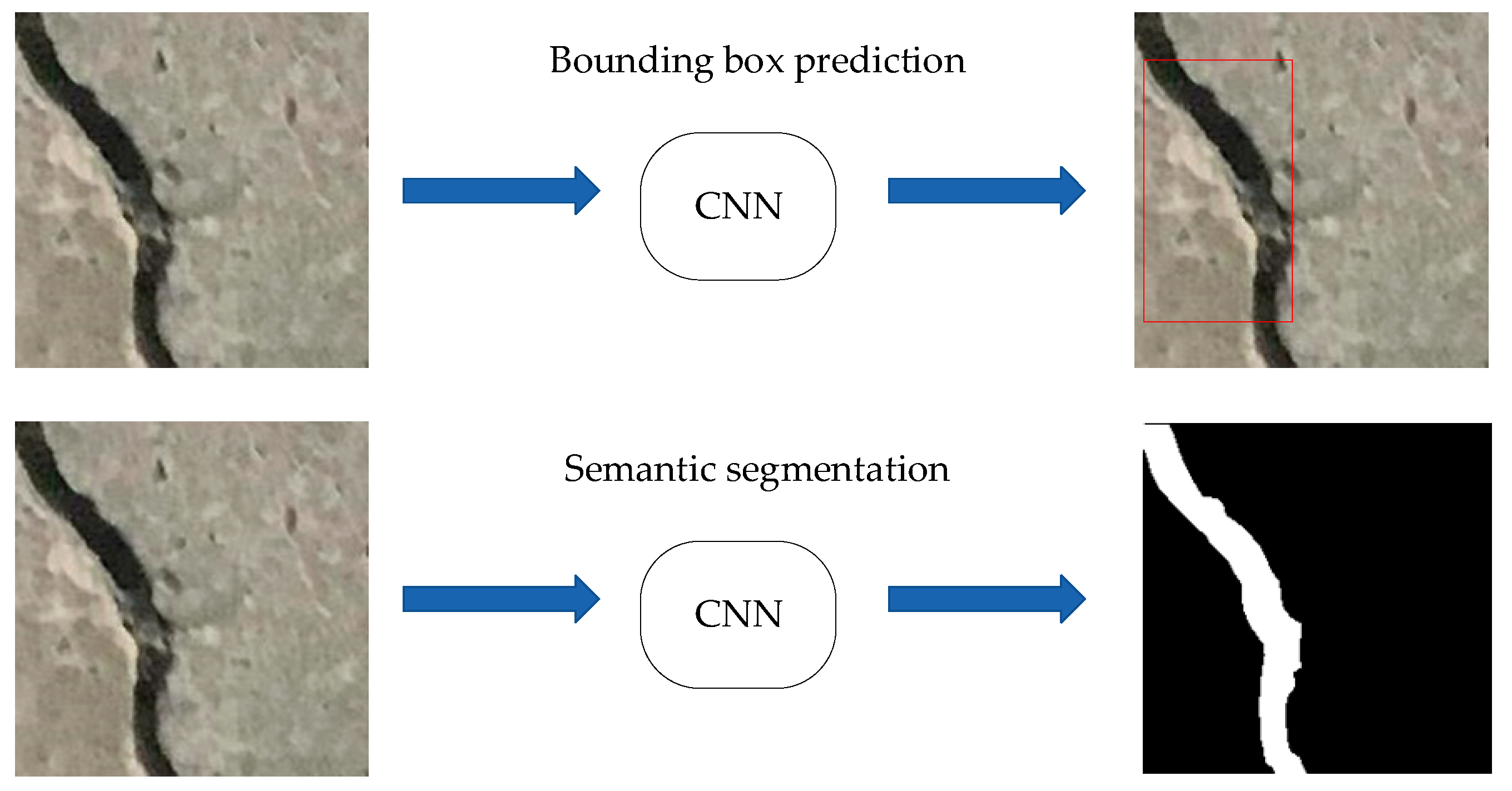
Generally, the detection task is to identify the targets and predict their coordinate positions. Concrete cracks have the characteristics of being long and bending, which make it difficult to predict the bounding box of the cracks. In addition, even if the bounding box of the crack is predicted, it usually contains a large amount of background information. Therefore, we transform concrete crack detection into semantics segmentation, that is, to distinguish whether the crack is a crack or not at the pixel level. As shown in Figure 1, a binary image is obtained after the input image is processed by CNN. The white part is concrete crack and the black part is non-crack. More details about the model are introduced in Section 3.1.
3.1. Model Description
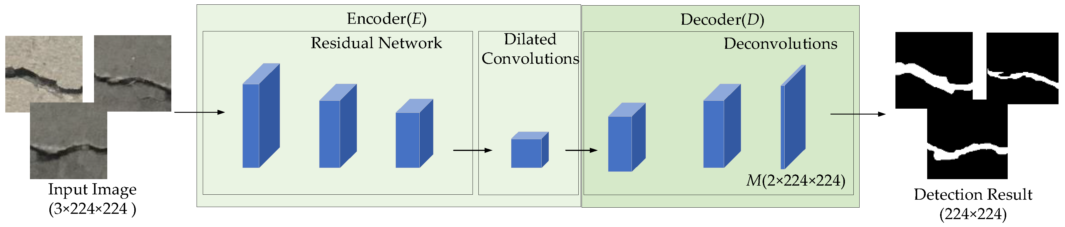
Inspired by FCN, a classical semantics segmentation algorithm, we propose a full convolution network based on dilated convolution for concrete crack detection, which consists of encoder E and decoder D. As shown in Figure 2, the encoder consists of residual network and dilated convolutions, while the decoder consists of deconvolutions. The encoder is used to extract feature maps from input images, which is a down-sampling process. After that, the feature extracted by encoder is enlarged by the decoder, and the final output is the probability maps with the same size as the input images. The whole model can be expressed as:
In Equation (1), represents the parameters of the encoding module E, represents the parameters of the decoding module D, M is a probability map with 2 channels, in which the value of each position represents the probability of crack and non-crack.
3.1.1. The Encoder
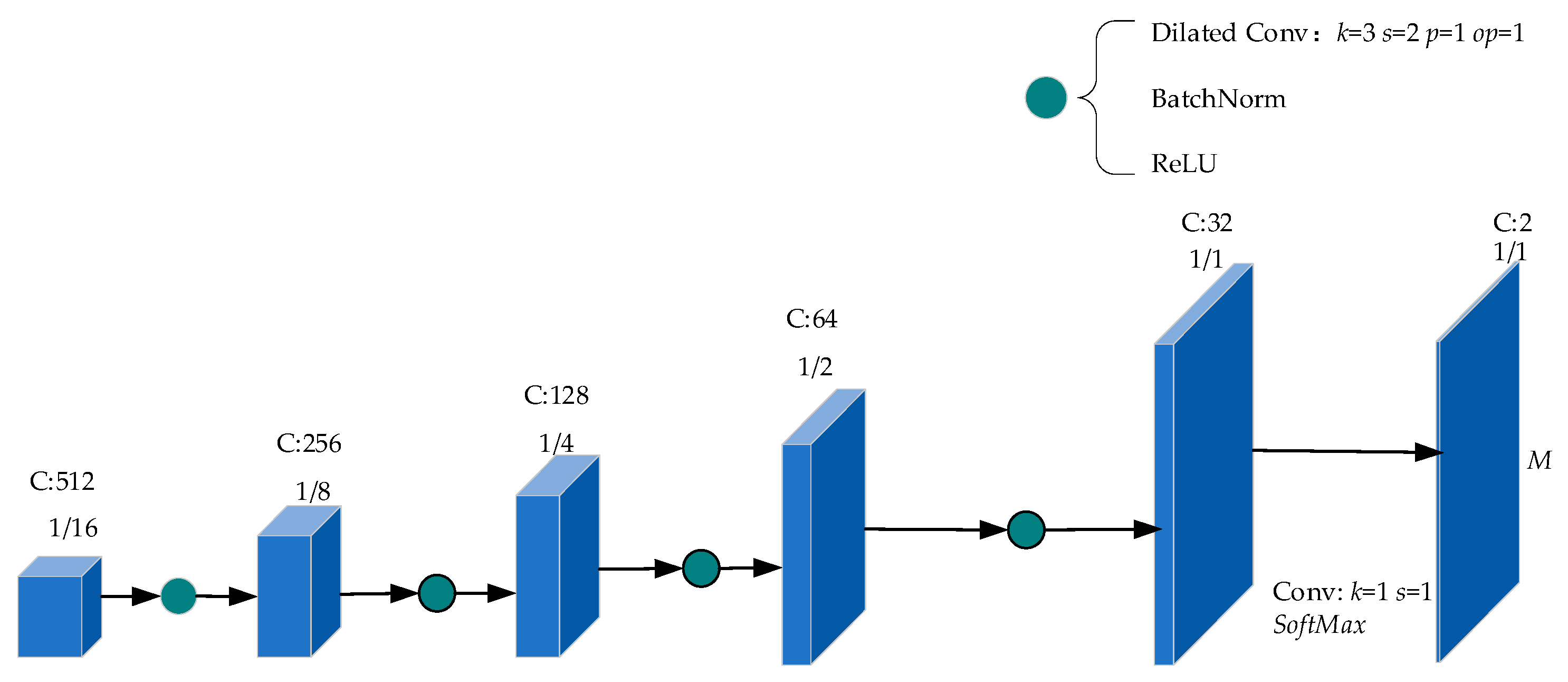
The encoder consisted of a residual network and several dilated convolutions as shown in Figure 3. The blue cube represents the feature maps. If there was no special explanation, the paddings of convolution and pooling were set to 0. As can be seen from Figure 3, the input image passed through a convolution layer with a convolution kernel k of size 7 × 7, a stride s of 2 and a padding p of 3, which was followed by BatchNorm, ReLU, and AvgPool. It should be noted that k, s, p of the AvgPool were 3, 2, and 1 respectively. The feature maps F0 obtained at this moment have 64 channels, the height and width of F0 are 1/4 of the input image. F1 with 64 Channels was obtained by extracting features from F0 through 2 residual blocks. It should be noted that F1 was the same size as F0. To obtain F2, F1 was processed by two residual blocks and AvgPool that had a kernel of size 2 × 2 and a stride of 2 in turn. Similar operations were performed on F2 to obtain F3. Then F3 was processed by two residual blocks to obtain F4, it should be noted that the process from F3 to F4 did not use AvgPool, which reduced information loss and retained more information. As the final output of the encoder, F5 had a complex manufacturing process, which was composed of the feature maps of the output of five branches: (1) The output was obtained by processing F2 with AvgPool that had a kernel k of size 2 × 2 and a stride s of 2; (2) The output was obtained by processing F4 with a composition layer composed of a BatchNorm, a ReLU, and a convolution that had a kernel k of size 1 × 1 and a stride s of 1. (3) The output was obtained by processing F4 with a composition layer composed of a BatchNorm, a ReLU, and a dilated convolution that had a kernel k of size 3 × 3, a stride s of 1, a padding p of 6, and a dilation rate d of 6. (4) The output was obtained by processing F4 with a composition layer composed of a BatchNorm, a ReLU, and a dilated convolution that had a kernel k of size 3 × 3, a stride s of 1, a padding p of 12, and a dilation rate d of 12. (5) The output was obtained by processing F4 with a composition layer composed of a BatchNorm, a ReLU, and a dilated convolution that had a kernel k of size 3 × 3, a stride s of 1, a padding p of 18, and a dilation rate d of 18. The feature maps obtained from these five branches were concatenated, and then a convolution with kernel k of size 1 × 1 and stride s of 1 was used for fusing the feature maps. After that, the feature maps flowed through BatchNorm and ReLU in turn. The height and width of the fused feature maps F5 are 1/16 of the input image. F5 served as the output of the encoder and the input of the decoder.
3.1.2. Residual Block
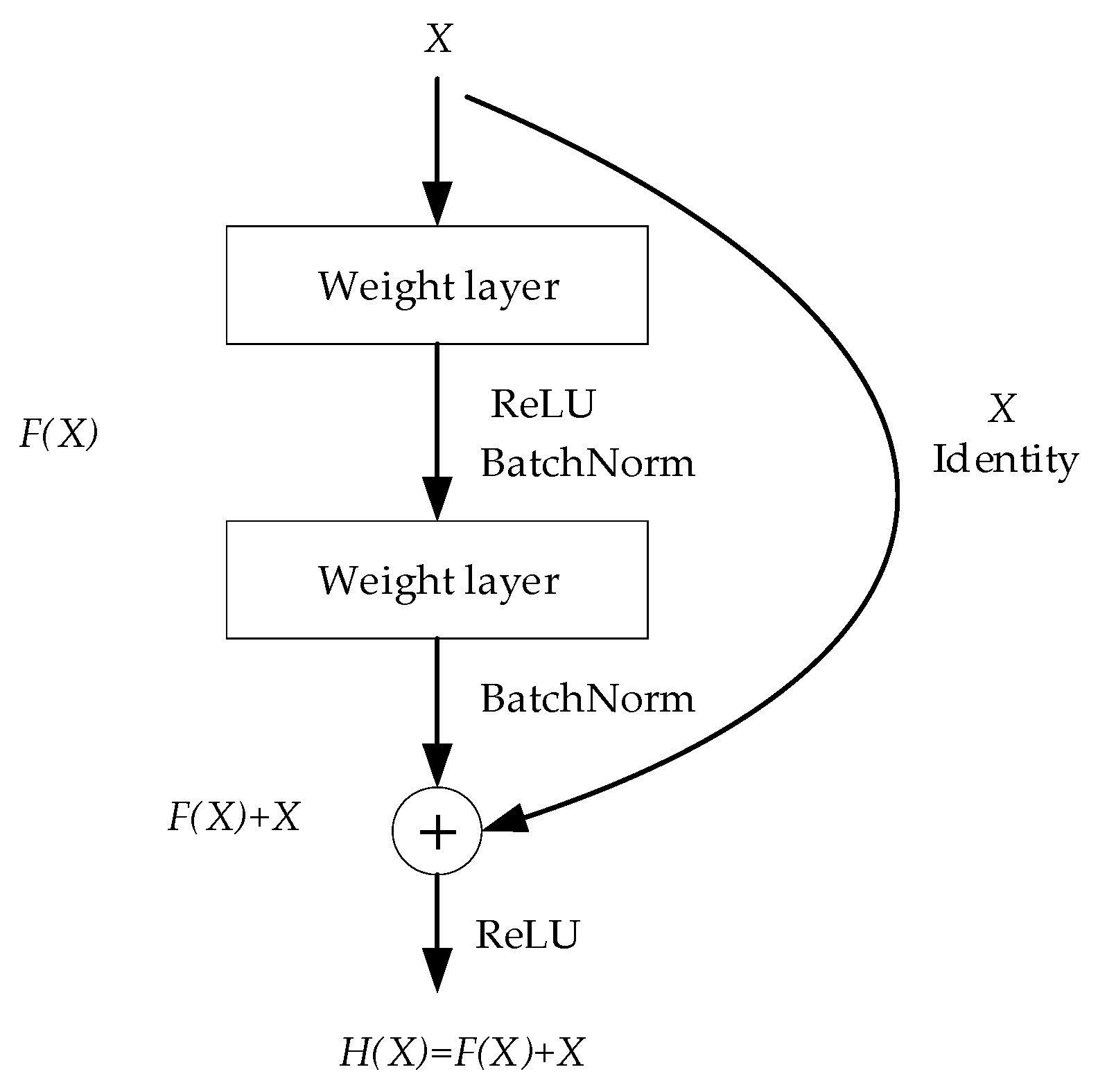
The residual network was proposed in 2015 [10], which is mainly to solve the problems of difficult training and network degradation in deep networks. The residual network is mainly composed of residual blocks. As shown in Figure 4, we denoted the expected mapping as. The stacked non-linear layers fit another mapping of . The design of the residual block was based on the assumption that it is easier to optimize the residual mapping than the original, unreferenced mapping. In extreme cases, if an identity mapping is optimal, it was much easier to push the residual to zero than to fit an identity mapping with stacked non-linear layers.
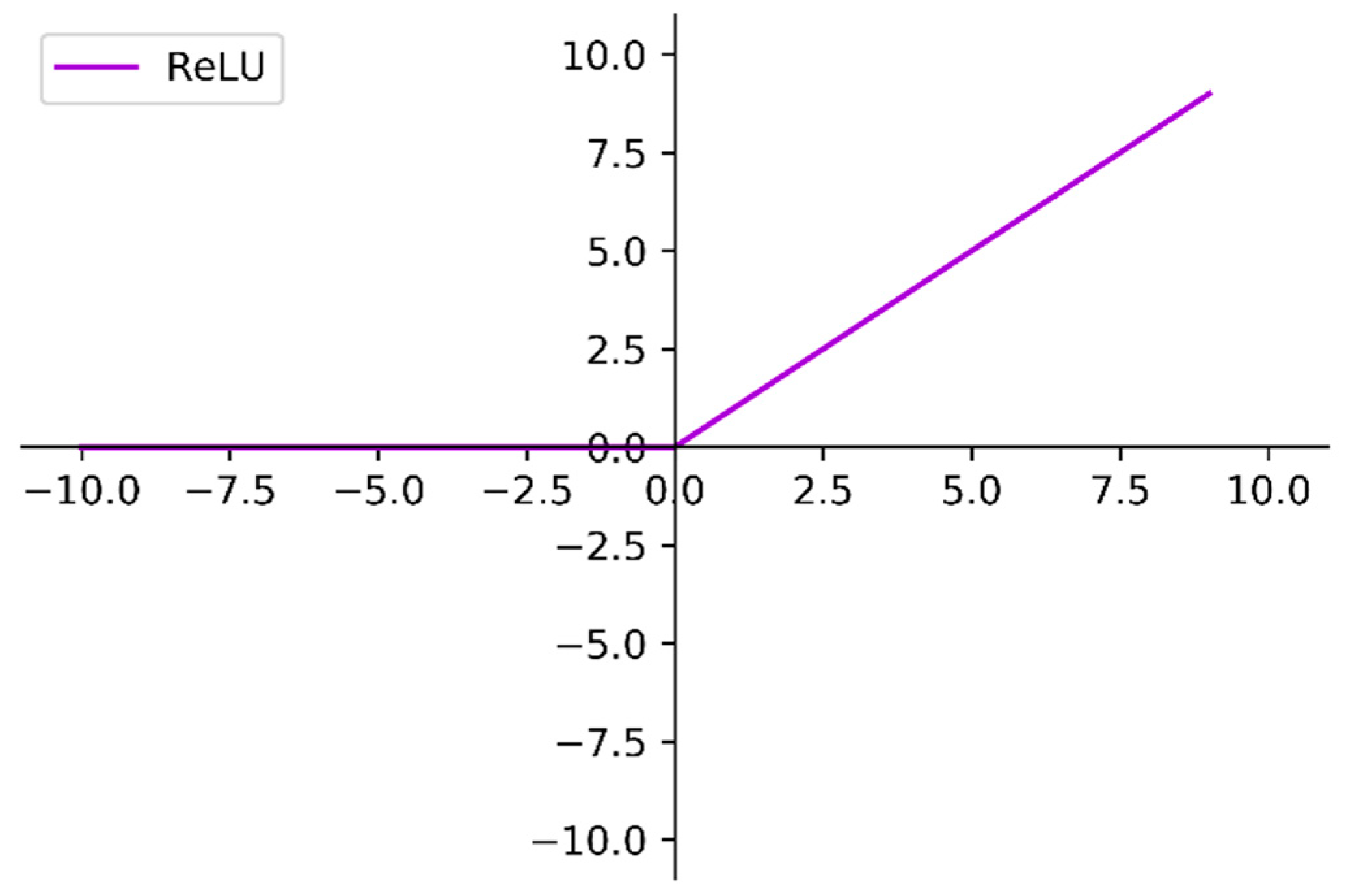
In the stacked nonlinear layers, the Rectified Linear Unit (ReLU) [47] was used as an activation function can improve the nonlinear expression capability of the network:
In Equation (2), represents the feature map in the network. After ReLU mapping, the values greater than 0 in the feature map are retained and the values less than or equal to 0 are set to 0. The visualization of ReLU is shown in Figure 5.
In the process of training, the distribution of data flowing in the network will gradually shift or change, thus slowing down the training process. In order to alleviate this problem, we used BatchNorm [48] technology to force the data back to more standard distribution. On the one hand, the problem of gradient disappearance was avoided. On the other hand, the training speed was greatly increased. The algorithm is described as follows: assume that B = {x1, x2, ..., xn} is a collection with n images, first calculate the expectation of B:
Then calculate the variance of B:
Then normalize B:
Finally, we get the normalized result by further processing :
In Equation (5), and are the parameters to be learned. A more detailed introduction to BatchNorm can be obtained from the literature [48].
3.1.3. Dilated Convolution
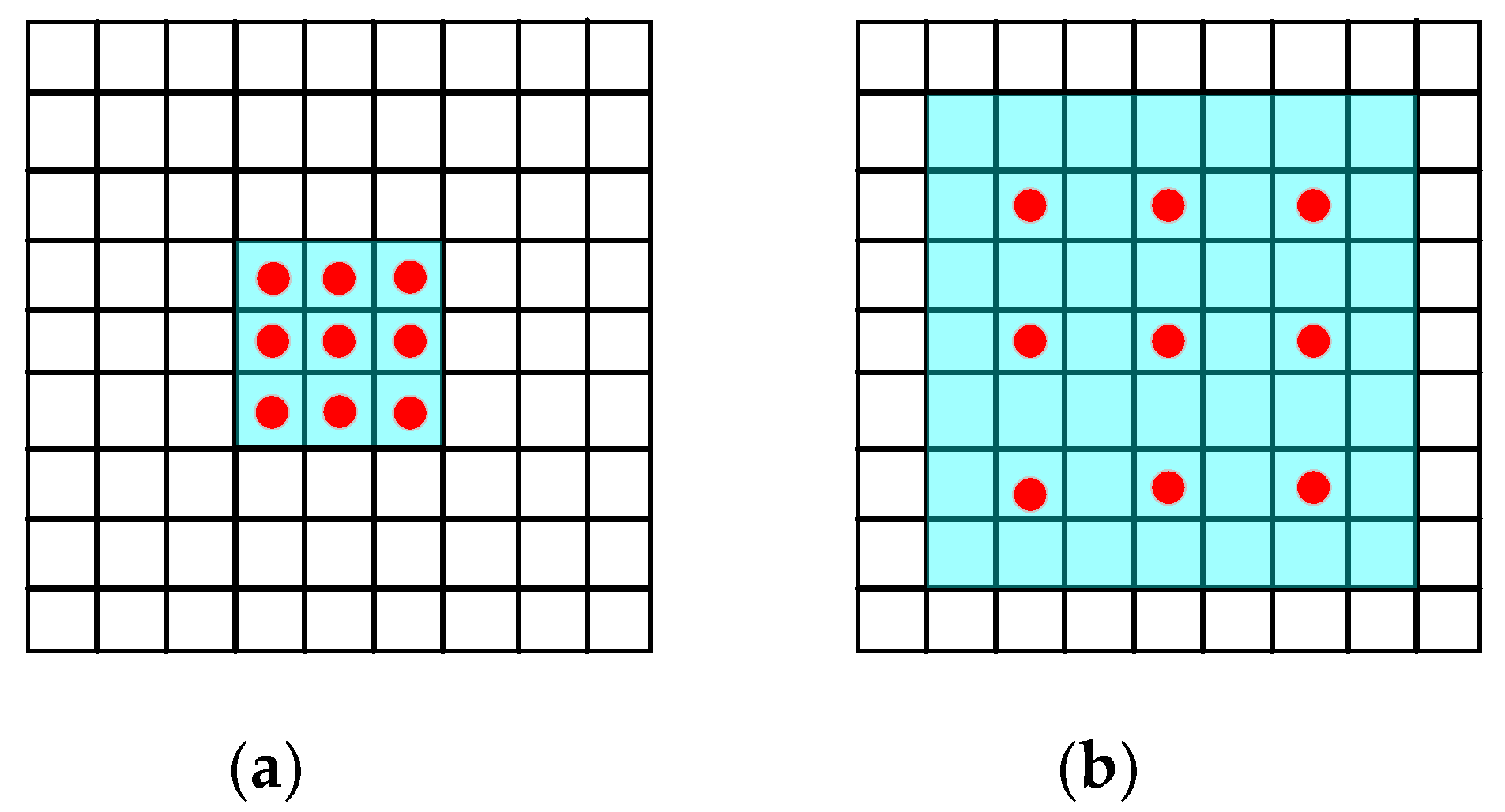
By increasing the dilation rate to control the receptive field of convolution on the traditional convolution, the dilated convolution [11] was designed, which is essentially the same as the traditional convolution. Different from the traditional convolution, the number of parameters of dilated convolution does not increase with the expansion of receptive field. The dilated convolution is shown in Figure 6. As can be seen from Figure 6b, the receptive field of the dilated convolution with a kernel k of size 3 × 3 and dilation rate d of 2 is of size 7 × 7, but has only 9 parameters, i.e., parts with red dot, which were actually involved in the calculation. The receptive field was controlled by the dilation rate of the dilated convolution. The dilated convolution degenerated into the traditional convolution when the dilation ratio d was set to 1, as shown in Figure 6a. Generally, to expand the receptive field, most networks usually use down-sampling, which is why pixel information is lost, resulting in errors. Dilated convolution can alleviate this problem. As shown in Figure 3, we did not perform down-sampling in the process from F3 to F4. We captured the feature maps of various receptive fields from F4 using dilated convolutions with various dilation rates, then obtained feature maps with more semantic information by fusing the feature maps with different receptive fields.
3.1.4. The Decoder
From the description above, it can be known that the feature maps F5 with 512 channels generated by the encoder are 1/16 of the input image. To enlarge the feature maps, we used decoder consist of stacked deconvolutions that are shown in Figure 7 to up-sample F5. For convenience of description, we refer to deconvolution, BatchNorm, and ReLU as an atomic operation, in which the feature maps flow through deconvolution, BatchNorm, and ReLU in turn. For each deconvolution, the convolution kernel k is size of size 3 × 3, the stride s is 2, the padding p is 1, and the output padding op is 1. Each deconvolution layer will double the size of the feature maps and reduce the number of channels by half. As can be seen from Figure 7, the feature map generated after 4 atomic operations is the same size as the input image. In order to obtain the required probability map M, we use a convolution layer with a convolution kernel k of 1, a stride s of 1 to map the feature maps into a 2-channel feature map, and then the SoftMax function is used to map the pixel category probability.
3.2. Loss Function
In general, the classification tasks use cross entropy loss:
In Equation (7), is the real category of pixels at the (i, j) position, . The quantity of neural network’s parameter is often too large, which easily leads to over-fitting and limits the generalization ability of the model. In order to alleviate this problem, we regularize the model parameters. The ultimate loss is as follows:
In Equation (8), represents the parameter of the model and represents the weight decay rate that is set to 1 × 10⁻⁵ in our experiment.
3.3. Parameter Optimization
Gradient descent is a classical algorithm for parameter optimization of deep convolution neural networks, which is described as follows:
In Equation (9), represents learning rate. As can be seen Equation (9), the updating of parameter a depends on the loss of the current batch image, which is unstable. To solve this problem, we introduce momentum.
In Equation (10), represents momentum, and represents velocity. In our experiment, is set to 0.001, is set to 0.9. It should be noted that is set to 0 at the beginning of training. Parameter of the model is updated according to Equation (10). From Equations (9) and (10), it can be found that the momentum simulates the inertia of moving objects, that is, the current update direction is obtained by fine-tuning the stored gradient through the gradient of the current training data, which can improve the stability of learning and speed up the training.
3.4. Training and Testing
In the experiment, the dataset is divided into training set, verification set and test set. First, the model is trained on the training set for 400 epochs. After the training, the model is tested on a test set. It should be mentioned that we use the mini-batch processing technology during the training, that is, in each iteration, we process a batch of samples at the same time, and the final loss is obtained by calculating the average loss of samples. The training and testing process are shown in Figure 8, and the training process is described as Algorithm 1.
| Algorithm 1 Model training algorithm |
| Input:I //Training sample set //The parameters of the model |
| 1: , , 2: for I = 1:400 do 3: // is obtained by randomly dividing I by batch size that is set // to 64 in our experiment. consists of all samples of one batch. 4: for s in S do 5: Calculate by forward processing s; 6: Calculate by using SoftMax to process ; 7: Calculate L according to Equation (7); 8: Calculate according to Equation (10); 9: Update according to Equation (11); 10: end for 11: end for 12: return |
| Output: // The parameters of the model |
4. Experiments
4.1. Dataset
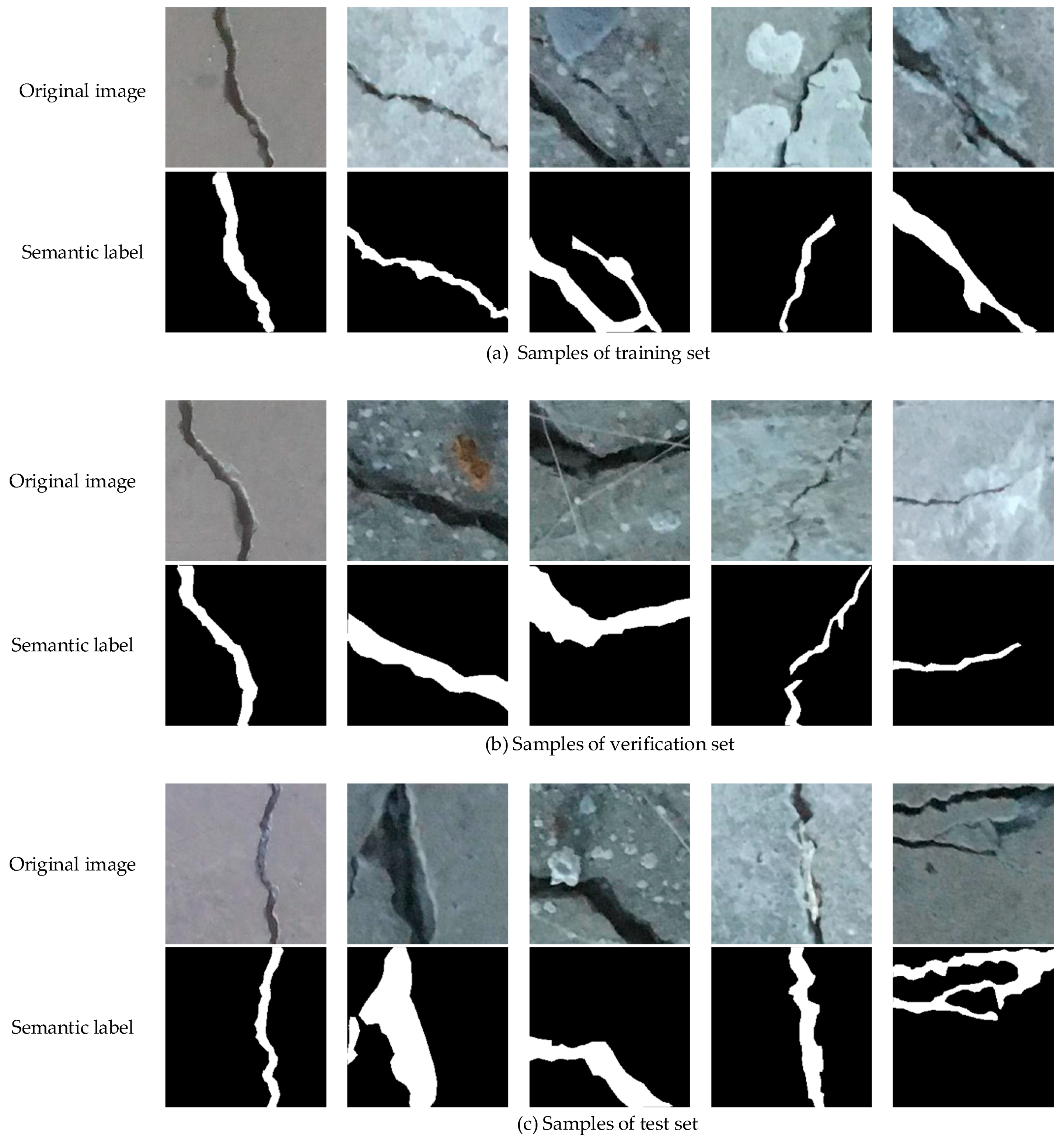
To evaluate the performance of the model, we used an open source concrete crack classification dataset [12], in which the images came from various METU campus buildings. The original dataset was divided into two categories, positive samples of cracks and negative samples of cracks. Each category had 20,000 images, with a total of 40,000 images. Each image had 227 × 227 pixels and 3 channels, namely RGB. Similar to some excellent concrete datasets with only image-level labels [49], the original dataset did not have pixel-level semantic labels and could not meet the requirements of segmentation tasks. Therefore, we created a suitable dataset based on the original dataset. The specific steps were as follows: (1) 600 images including cracks were selected from the dataset. (2) The 600 images were manually labeled to obtain pixel-level semantic labels. As shown in Figure 9, the black part is the background and the white part is the crack. It should be noted that all the semantic labels were marked by 4 students using the tool named “labelme” for about 2 weeks. In order to ensure the accuracy of the labels as much as possible, a more professional person made the final examination. (3) The dataset is divided into three parts: training set, verification set and test set, in which the training set was allocated 400 samples and the verification set and test set were both 100 samples. Some samples of different sets are shown in Figure 9. We used the training set to train the model and the verification set to observe the performance of the model during the training. The model parameters were saved after completing the training and the performance of the model was evaluated using test set.
4.2. Evaluation Indicators
In order to effectively evaluate the performance of the model, we introduced some commonly-used indicators [34] in semantic segmentation as the performance indicators of the model. These indicators included PA (Pixel Accuracy), MPA (Mean Pixel Accuracy), MIoU (Mean Intersection over Union), and FWIoU (Frequency Weighted Intersection over Union). We assumed that there were a total of k + 1 classes, from L0 to Lk, which contained the background. represents the number of pixels that belong to class i but are predicted to be class j. PA is the proportion of correctly marked pixels to total pixels:
MAP is a simple promotion of PA, which calculates the proportion of correctly classified pixels in each class, and then computes the average of all categories:
MIoU, as a standard measure of semantic segmentation, calculates the ratio of intersection and union of two sets, which can be transformed into the sum of positive true number ratio, false negative number ratio and false positive number ratio. IoU is calculated on each category and then averaged:
FWIoU is an improvement on MIoU, which weights the importance of each class according to its frequency of occurrence.
4.3. Experimental Preparation
4.3.1. Experimental Environment
All experiments were implemented on a GPU server. The CPU of the GGP server was Intel(R) Xeon(R) CPU E5-2640 v4, its main frequency was 2.40 GHz, the memory was 128 GB, the graphics card was GeForce GTX 1080Ti, and the display memory was 11 GB. The operating system was Ubuntu 16.04.5 LTS, and the open source framework for deep learning we used was pytorch1.0.1.
4.3.2. Experimental Design
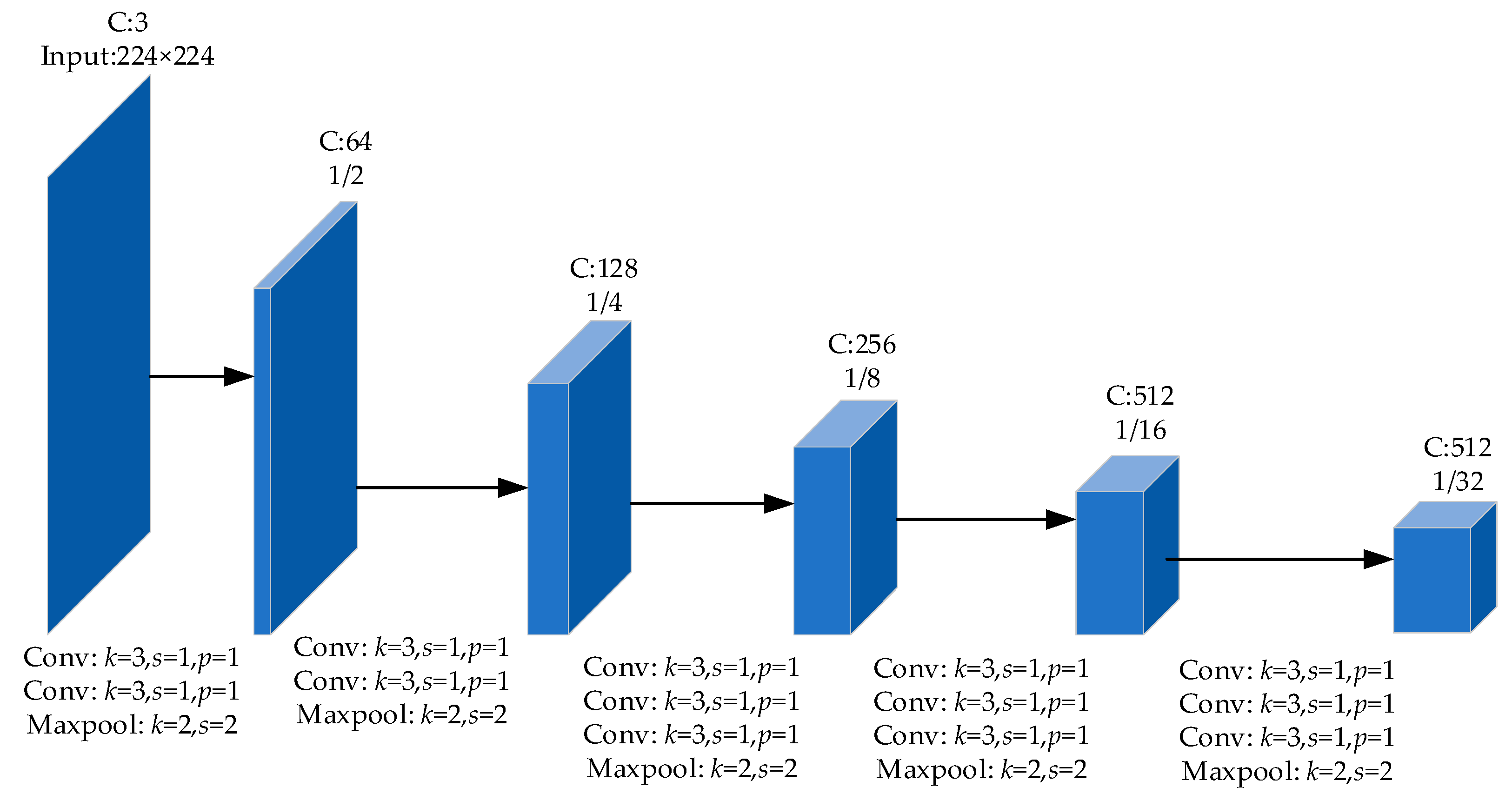
In order to select the backbone network and verify the effectiveness of the algorithm, we designed four models for experiments: (1) The model called FCN-Resnet-18, which removed dilated convolution and feature fusion, and only retained residual network as encoder. As shown in Figure 3, the feature maps F4 were the output of the encoder. (2) The model called FCN-Resnet-50, which is similar to FCN-Resnet-18. The only difference between FCN-Resnet-50 and FCN-Resnet-18 is that the residual network in FCN-Resnet-50 has more layers. In FCN-Resnet-50, we utilized Resnet-50 as the backbone network, and the specific structure can be seen from [10]. It should be noted that AvgPool was used for down-sampling, which ensured that the down-samplings of Renset-50 were consistent with down-samplings of Resnet-18 we used. (3) The model called FCN-VGG, which is a classical semantic segmentation algorithm and uses VGG16 as an encoder. (4) The proposed model, which combines Resnet-18 and dilated convolutions that have different dilation rates as the encoder. That is to say, the proposed model is an improved version of FCN-Resnet-18. The encoder structure is shown in Figure 3. It should be further explained that, unlike the proposed model, FCN-Resnet-18 and FCN-Resnet-50 performed down-sampling before outputting the feature maps F4, that is, the feature maps output from the encoder of FCN-Resnet-18 and FCN-Resnet-50 were 1/32 of the input image. Similarly, the feature maps output by the encoder of FCN-VGG were 1/32 of the input image. In order to be able to access the up-sampling module, a deconvolution layer was used to enlarge the feature maps with a size of 1/32 of the input image, so that their size became 1/16 of the input image after the deconvolution layer. It should be noted that the deconvolution layer used includes deconvolution, BatchNorm, and ReLU. The encoder VGG is shown in Figure 10. The comparison of parameters, layers, and training time of different models is show in Table 1. It should be noted that the training time in seconds refers to the time required to complete training of 400 epochs. In addition, the number of network layers we counted included convolution layer, average pooling layer, and deconvolution layer.
4.3.3. The Hyper Parameters
In our experiment, the parameters that needed to be set manually included learning rate, weight decay rate, batch size, and the epochs of training. As mentioned before, we set the learning rate to 0.001 and the weight decay rate to 1 × 10⁻⁵. In order to fully train the parameters of the network, we set the epochs of training to 400 and the batch size to 64. It should be noted that the super parameters used in all models are the same to ensure the fairness of the experiment as much as possible.
4.4. Results and Analysis
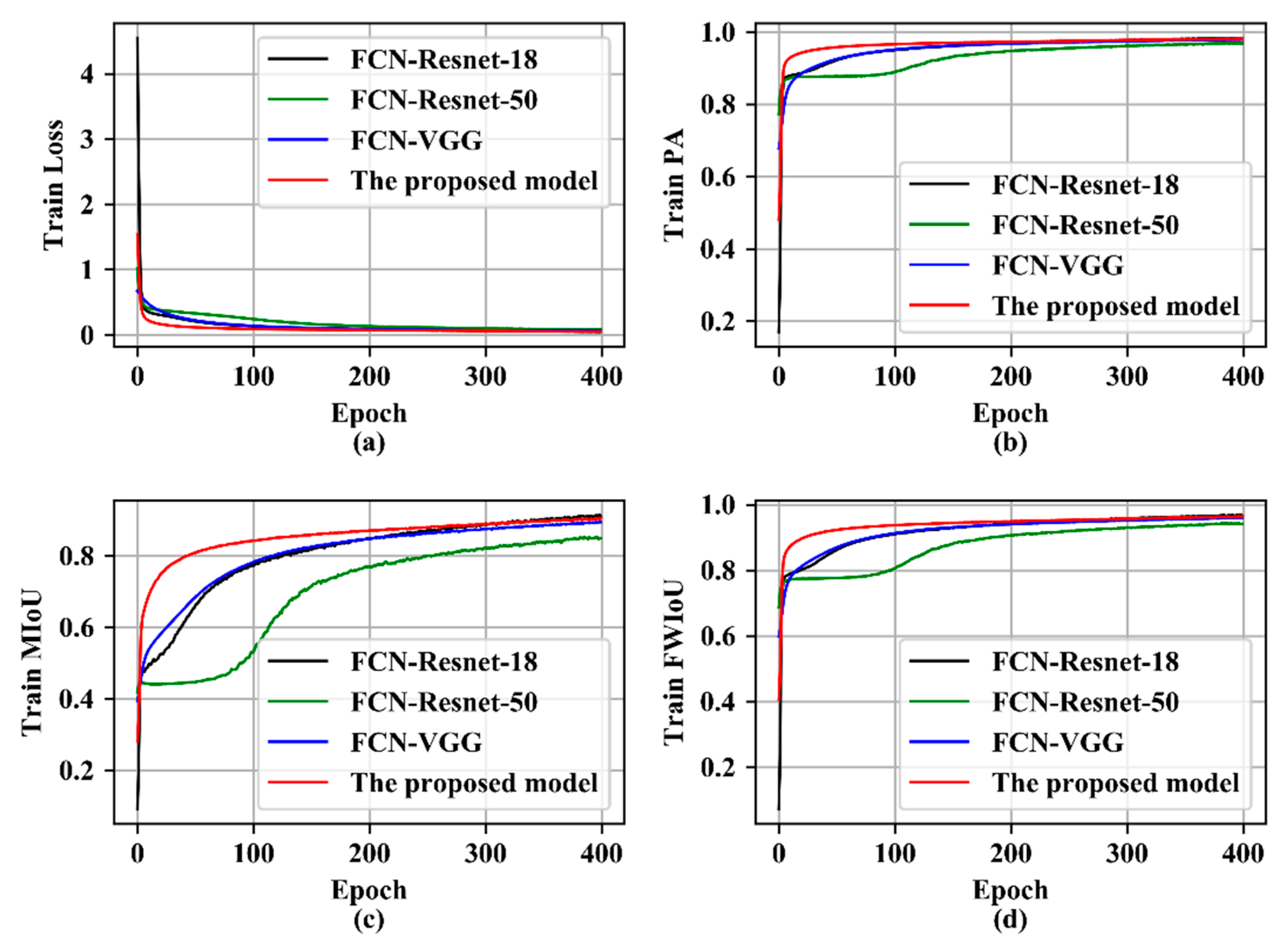
Performance on the training set. According to the indicators shown in Figure 11, the proposed model performs best. Figure 11a shows the convergence of each model in the training phase. It can be found that compared with other models, the loss of the proposed model can be reduced very low after a small number of epochs. This shows that, on the one hand, the proposed model has stronger fitting ability, on the other hand, the proposed model can generate more efficient gradient information. From the change of PA shown in Figure 11b, it can be found that the PA of the proposed model rises fastest, which also shows that the proposed model has stronger fitting ability. As can be seen from Figure 11c, the MIoU of FCN-Resnet-50 is the worst, and other models are almost the same at the 400th epoch. It should also be pointed out that the proposed model achieves a higher MIoU at a faster speed. The same situation also occurs in Figure 11d. As can be seen from Figure 11, all models can fit the training dataset, that is, as the training progresses, each model can learn something from the dataset. This shows that it is feasible to model concrete crack detection as a semantic segmentation of cracks. Compared with other models, the proposed model has a faster learning speed. We speculate that the design of multiple branches makes the model accept more gradient information, thus speeding up the fitting speed. Although FCN-Resnet-50 has more layers, its performance is relatively poor, which shows that deeper networks are not necessarily better than shallow networks. We suspect that the degradation of FCN-Resnet-50 may be the cause. The proposed model is improved on the basis of FCN-Resnet-18, and its performance is better than FCN-Resnet-18, which proves that the dilated convolutions with different dilation rates and the multi-branch fusion strategy are effective.
4.4.1. Performance on Validation Set
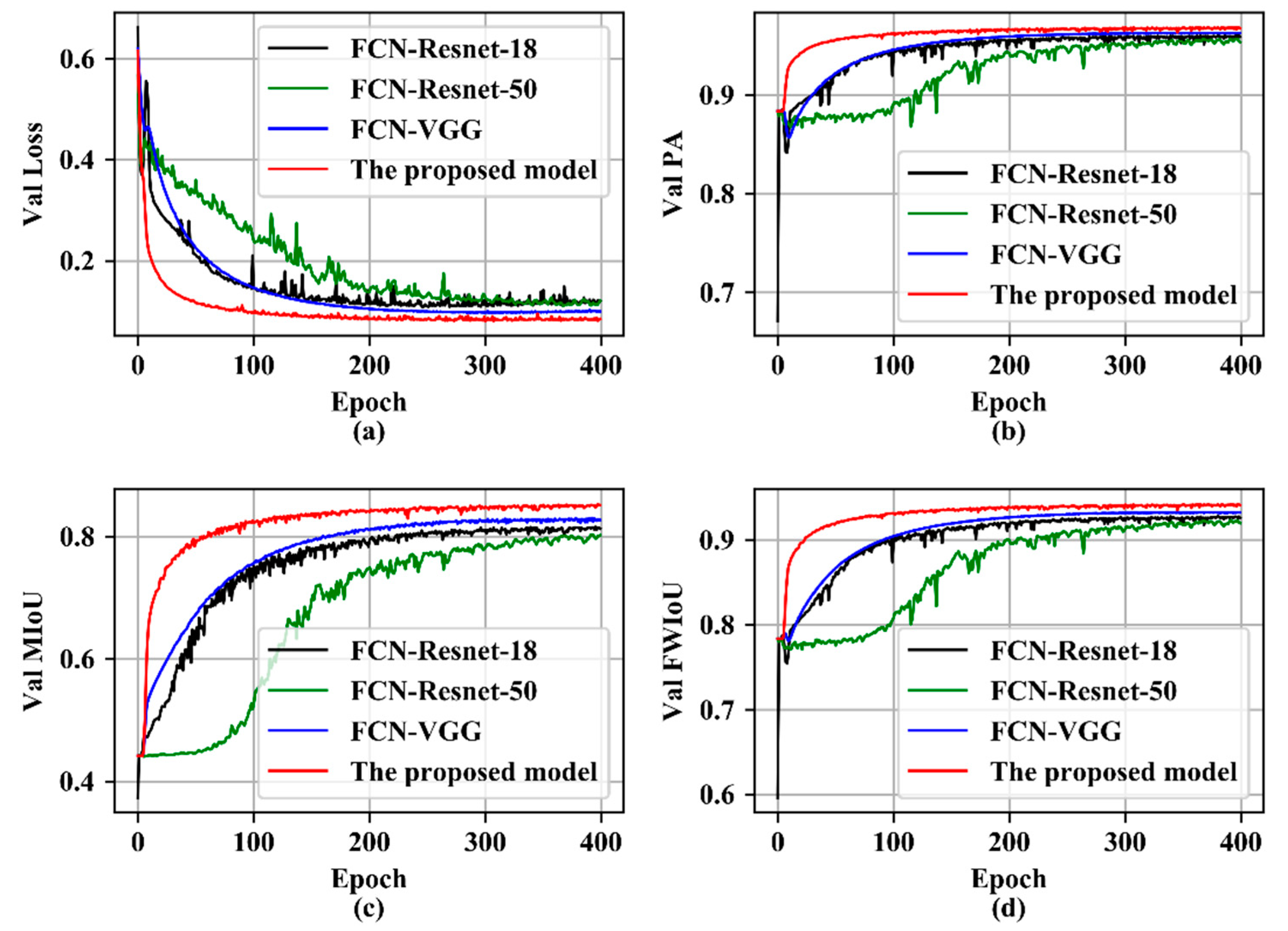
Compared with the performance on the training set, the performance on the verification set can better reflect the generalization ability of the model. According to the indexes of Figure 12, the proposed model performed better on the verification set. As shown in Figure 12a, the loss of the proposed model on the verification set decreased fastest. After training of 400 epochs, the loss of the proposed model was the lowest, followed by FCN-VGG. The final losses of FCN-Resnet-18 and FCN-Resnet-50 were the same. In the training process, the losses of FCN-Resnet-18 and FCN-Resnet-50 had great fluctuations. Although Figure 11a reports that all models had similar losses, it can be seen from Figure 12a that the generalization ability of FCN-Resnet-18 and FCN-Resnet-50 is deficient. As shown in Figure 12b, the PA of FCN-Resnet-18 and FCN-Resnet-50 had obvious fluctuations. After training of 400 epochs, the PA of FCN-Resnet-18, FCN-Resnet-50 and FCN-VGG were similar, but there was still a gap with the proposed model. From the situation shown in Figure 12c, the performance difference of each model was more obvious. The best was the proposed model, followed by FCN-VGG, then FCN-Resnet-18, and finally FCN-Resnet-50. On the verification set, both the proposed model and FCN-VGG were relatively stable, while the proposed model could achieve better MIoU. The same situation also occurred in FWIoU, as shown in Figure 12d. By comparing Figure 12 with Figure 11, it is obvious that the generalization ability of the proposed model is the best, which proves the effectiveness of dilated convolutions with different dilation rates and the multi-branch fusion strategy.
4.4.2. Performance on Test Sets
In order to further verify the performance of the model, all models are tested on the test set. The compared model parameters are all obtained through the training of 400 epochs on the training set. The test results are shown in Table 2. As can be seen from Table 1, although FCN-Resnet-50 has more layers than FCN-Resnet-18, FCN-Resnet-18 was more competitive than FCN-Resnet-50. Compared with FCN-VGG, the performance of FCN-Resnet-18 was slightly worse. By designing dilated convolutions with different dilation rates and a multi-branch fusion strategy to improve FCN-Resnet-18, the proposed model had better performance. Compared with FCN-Resnet-18, all Indicators were improved, especially MIoU. More importantly, the performance of the improved model exceeded that of FCN-VGG, which proves the effectiveness of the dilated convolutions with different dilation rates and multi-branch feature fusion strategy.
4.4.3. Effect Shown
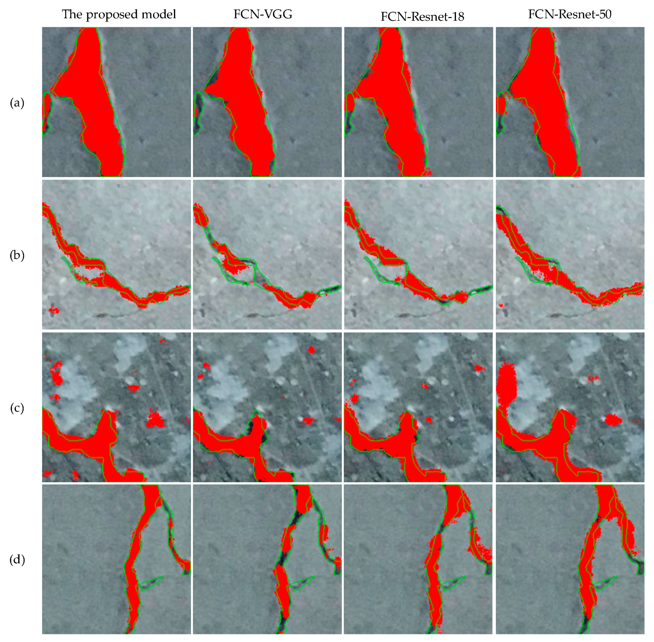
As shown in Figure 13, the segmentation results of each model. The pixels surrounded by the green curve are manually marked pixels belonging to cracks. The red part is the pixel inferred by the model as belonging to the crack. It should be noted that the segmentation result of the model is a binary image, that is, the pixels not belonging to cracks are marked as 0 and the pixels belonging to cracks are marked as 1. In order to obtain the display effect as shown in the figure, we used the segmented binary image as a mask. Corresponding to the position of 1 in the mask, the R channel of the original image is set to 255, while the G channel and B channel are both set to 0. As can be seen from Figure 13, the segmentation result of the proposed model was the best. As shown in Figure 13a, for cracks with large area, several models can segment cracks well. It should be pointed out that the segmentation result of the proposed model was closer to that of manual annotation. In addition, it can be seen in Figure 13a that FCN-VGG, FCN-Resnet-18 and FCN-Resnet-50 did not segment cracks with small area well, especially FCN-VGG. The same situation also occurs in Figure 13b,d. The reason is that excessive down-sampling leads to loss of details, thus the original semantic information cannot be decoded. Compared with other models, the proposed model has one less down-sampling operation, then the dilated convolutions with different dilation rates and a multi-branch fusion strategy were designed so that the receptive field was expanded while the detail information was preserved, which alleviated the problem of detail loss to some extent. As shown in Figure 13b, for the proposed model, some fine cracks could also be segmented. It should be pointed out that the proposed model also had incomplete segmentation of fine cracks, as shown in Figure 13d, which also shows that the proposed model had the problem of missing details, but it was not as serious as other models. As shown in Figure 13c, for scenes with relatively complex backgrounds, each model had the problem of wrong segmentation. The reason is that our dataset is relatively simple and lacks training samples under complex background, thus causing erroneous segmentation.
5. Conclusions
The detection of concrete cracks has extremely important practical application value, which can greatly reduce human and material resources. In order to accurately obtain the location and shape of concrete cracks, we modeled crack detection as a semantic segmentation task. Considering the loss of details caused by down-sampling in the traditional concrete crack segmentation algorithm based on FCN, we designed dilated convolutions with different dilation rates and a multi-branch fusion strategy. Because Resnet-18 has fewer parameters and requires fewer computing resources, we used Resnet-18 as the basic network. After removing the last down-sampling of Resnet-18, we introduced dilated convolution with different dilation rates, and then fused the features of different branches. Experiments showed that the design of dilated convolution with different dilation rates and the multi-branch feature fusion strategy can alleviate the problem of detail loss to some extent. From the experimental results of FCN-Resnet-18 and FCN-Resnet-50, the segmentation performance did not improve with the increase of network layers. Because the dataset is relatively simple and lacks semantic label samples with complex backgrounds, the proposed model suffers from erroneous segmentation when dealing with images with complex backgrounds. In addition, our model still has a lot of room for improvement for details loss. Our future work will explore the construction of a complex dataset with pixel semantic labels.
Author Contributions
Conceptualization, J.Z. and C.L.; Methodology, C.L.; Software, C.L.; Validation, C.L., J.Z, L.W., J.W., and X.-G.Y.; Formal Analysis, C.L.; Investigation, C.L.; Resources, L.W.; Data Curation, X.Y.; Writing—Original Draft Preparation, C.L.; Writing—Review and Editing, J.Z.; Visualization, C.L.; Supervision, J.Z.; Funding Acquisition, J.W.
Funding
This research was funded in part by the National Natural Science Foundation of China under Grant Nos. 61772454, 61811540410 and 61811530332, the Scientific Research Fund of Hunan Provincial Education Department under Grant No. 16A008, the Postgraduate Scientific Research Innovation Fund of Hunan Province under Grant No. CX2018B565, the "Double First-class" International Cooperation and Development Scientific Research Project of Changsha University of Science and Technology under Grant No. 2019IC34, and the Postgraduate Training Innovation Base Construction Project of Hunan Province under Grant No. 2017-451-30.
Acknowledgments
We are grateful to Çağlar Fırat Özgenel who provide the dataset (Concrete Crack Images for Classification, http://dx.doi.org/10.17632/5y9wdsg2zt.1).
Conflicts of Interest
The authors declare no conflict of interest.
References
- Nhat-Duc, H. Detection of Surface Crack in Building Structures Using Image Processing Technique with an Improved Otsu Method for Image Thresholding. Adv. Civ. Eng. 2018. [Google Scholar] [CrossRef]
- Liu, X.; Ai, Y.; Scherer, S. Robust Image-Based Crack Detection in Concrete Structure Using Multi-Scale Enhancement and Visual Features. In Proceedings of the IEEE International Conference on Image Processing, Beijing, China, 17–20 September 2017; pp. 2304–2308. [Google Scholar]
- Dorafshan, S.; Thomas, R.J.; Maguire, M. Benchmarking Image Processing Algorithms for Unmanned Aerial System-Assisted Crack Detection in Concrete Structures. Infrastructures 2019, 4, 19. [Google Scholar] [CrossRef]
- Cha, Y.; Choi, W.; Büyüköztürk, O. Deep Learning-Based Crack Damage Detection Using Convolutional Neural Networks. Comput.-Aided Civil Infrastruct. Eng. 2017, 32, 361–378. [Google Scholar] [CrossRef]
- Dorafshan, S.; Thomas, R.; Coopmans, C.; Maguire, M. Deep Learning Neural Networks for sUAS-Assisted Structural Inspections: Feasibility and Application. In Proceedings of the International Conference on Unmanned Aircraft Systems, 650 N. Pearl Str., Dallas, TX, USA, 2–15 June 2018; pp. 874–882. [Google Scholar]
- Cha, Y.; Choi, W.; Suh, G.; Mahmoudkhani, S.; Büyüköztürk, O. Autonomous Structural Visual Inspection Using Region-Based Deep Learning for Detecting Multiple Damage Types. Comput.-Aided Civil Infrastruct. Eng. 2018, 33, 731–747. [Google Scholar] [CrossRef]
- Long, J.; Shelhamer, E.; Darrell, T. Fully Convolutional Networks for Semantic Segmentation. In Proceedings of the IEEE Conference on Computer Vision and Pattern Recognition, Boston, MA, USA, 7–12 June 2015; pp. 3431–3440. [Google Scholar]
- Teichmann, M.; Weber, M.; Zöllner, M.; Cipolla, R.; Urtasun, R. MultiNet: Real-time Joint Semantic Reasoning for Autonomous Driving. In Proceedings of the IEEE Intelligent Vehicles Symposium, Changshu, Suzhou, China, 26–30 September 2018; pp. 1013–1020. [Google Scholar]
- Kampffmeyer, M.; Salberg, A.; Jenssen, R. Semantic Segmentation of Small Objects and Modeling of Uncertainty in Urban Remote Sensing Images Using Deep Convolutional Neural Networks. In Proceedings of the IEEE Conference on Computer Vision and Pattern Recognition Workshops, Las Vegas, NV, USA, 26–30 June 2016; pp. 680–688. [Google Scholar]
- He, K.; Zhang, X.; Ren, S.; Ren, S. Deep Residual Learning for Image Recognition. In Proceedings of the IEEE Conference on Computer Vision and Pattern Recognition, Las Vegas, NV, USA, 26–30 June 2016; pp. 770–778. [Google Scholar]
- Chen, L.; Papandreou, G.; Schroff, F.; Adam, H. Rethinking Atrous Convolution for Semantic Image Segmentation. arXiv 2017, arXiv:1706.05587. [Google Scholar]
- Concrete Crack Images for Classification. Available online: https://data.mendeley.com/datasets/5y9wdsg2zt/1 (accessed on 1 June 2019).
- Alberto, G.; Sergio, O.; Sergiu, O.; Victor, V.; Jose, G. A Review on Deep Learning Techniques Applied to Semantic Segmentation. arXiv 2017, arXiv:1704.06857. [Google Scholar]
- Ng, H.; Hashim, M.; Jaw, S. Building Concrete Cracks Detection Using Image-Based Nondestructive Geotechnical Technique. In Proceedings of the Asian Conference on Remote Sensing 2014: Sensing for Reintegration of Societies, Nay Pyi Taw, Myanmar, 27–31 October 2014. [Google Scholar]
- Taghavipour, S.; Kharkovsky, S.; Kang, W.; Samali, B.; Mirza, O. Detection and Monitoring of Flexural Cracks in Reinforced Concrete Beams Using Mounted Smart Aggregate Transducers. Smart Mater. Struct. 2017, 26. [Google Scholar] [CrossRef]
- Voigt, B.; Bordin, F.; Gorkos, P.; Veronez, M. Detection of Cracks and Loss of Mass in Concrete Through 3D Point Clouds Generated by Terrestrial Laser Scanner. In Proceedings of the International Conference on Bridge Maintenance, Safety and Management, Foz do Iguaçu, Brazil, 26–30 June 2016; pp. 1840–1845. [Google Scholar]
- Chen, Y.; Wang, J.; Xia, R.; Zhang, Q.; Cao, Z.; Yang, K. The Visual Object Tracking Algorithm Research Based on Adaptive Combination Kernel. J. Ambient Intell. Humaniz. Comput. 2019, (in press). [Google Scholar] [CrossRef]
- Zhang, J.; Jin, X.; Sun, J.; Wang, J.; Sangaiah, A. Spatial and Semantic Convolutional Features for Robust Visual Object Tracking. Multimed. Tools Appl. 2018, in press. [Google Scholar] [CrossRef]
- Zhang, J.; Wu, Y.; Jin, X.; Li, F.; Wang, J. A Fast Object Tracker Based on Integrated Multiple Features and Dynamic Learning Rate. Math. Probl. Eng. 2018, 2018, 1–14. [Google Scholar] [CrossRef] [Green Version]
- Zhang, J.; Jin, X.; Sun, J.; Wang, J.; Li, K. Dual Model Learning Combined with Multiple Feature Selection for Accurate Visual Tracking. IEEE Access. 2019, 7, 43956–43969. [Google Scholar] [CrossRef]
- Zhang, J.; Lu, C.; Li, X.; K, H.; W, J. A Full Convolutional Network Based on DenseNet for Remote Sensing Scene Classification. Math. Biosci. Eng. 2019, 16, 3345–3367. [Google Scholar] [CrossRef]
- Gatys, L.; Ecker, A.; Bethge, M. Image Style Transfer Using Convolutional Neural Networks. In Proceedings of the IEEE Conference on Computer Vision and Pattern Recognition, Las Vegas, NV, USA, 26–30 June 2016; pp. 2414–2423. [Google Scholar]
- Calderón, L.; Bairan, J. Crack Detection in Concrete Elements from RGB Pictures Using Modified Line Detection Kernels. In Proceedings of the Intelligent Systems Conference, London, UK, 7–8 September 2017; pp. 799–805. [Google Scholar]
- Dinh, T.; Ha, Q.; La, H. Computer Vision-Based Method for Concrete Crack Detection. In Proceedings of the International Conference on Control, Automation, Robotics and Vision, Phuket, Thailand, 13–15 November 2016. [Google Scholar]
- Qu, Z.; Guo, Y.; Ju, F.; Liu, L.; Lin, L.D. The Algorithm of Accelerated Cracks Detection and Extracting Skeleton by Direction Chain Code in Concrete Surface Image. Imaging Sci. J. 2016, 64, 119–130. [Google Scholar] [CrossRef]
- Karen, S.; Andrew, Z. Very Deep Convolutional Networks for Large-Scale Image Recognition. arXiv 2015, arXiv:1409.1556. [Google Scholar]
- Zhou, S.; Liang, W.; Li, J.; Kim, J. Improved VGG Model for Road Traffic Sign Recognition. CMC-Comput. Mat. Contin. 2018, 57, 11–24. [Google Scholar] [CrossRef]
- Russakovsky, O.; Deng, J.; Su, H.; Krause, J.; Satheesh, S.; Ma, S.; Huang, Z.; Karpathy, A.; Khosla, A.; Bernstein, M.; et al. ImageNet Large Scale Visual Recognition Challenge. Int. J. Comput. Vis. 2015, 115, 211–252. [Google Scholar] [CrossRef] [Green Version]
- Ren, S.; He, K.; Girshick, R.; Sun, J. Faster R-CNN: Towards Real-Time Object Detection with Region Proposal Networks. IEEE Trans. Pattern Anal. Mach. Intell. 2017, 39, 1137–1149. [Google Scholar] [CrossRef] [Green Version]
- Zhou, S.; Ke, M.; Luo, P. Multi-Camera Transfer GAN for Person Re-Identification. J. Vis. Commun. Image Represent. 2019, 59, 393–400. [Google Scholar] [CrossRef]
- Tu, Y.; Lin, Y.; Wang, J.; Kim, J. Semi-Supervised Learning with Generative Adversarial Networks on Digital Signal Modulation Classification. CMC-Comput. Mat. Contin. 2018, 55, 243–254. [Google Scholar]
- Zeng, D.; Dai, Y.; Li, F.; Sherratt, R.; Wang, J. Adversarial Learning for Distant Supervised Relation Extraction. CMC-Comput. Mat. Contin. 2018, 55, 121–136. [Google Scholar]
- Long, M.; Zeng, Y. Detecting Iris Liveness with Batch Normalized Convolutional Neural Network. CMC-Comput. Mat. Contin. 2019, 58, 493–504. [Google Scholar] [CrossRef]
- Kasthurirangan, G. Deep Learning in Data-Driven Pavement Image Analysis and Automated Distress Detection: A Review. Data 2018, 3, 28. [Google Scholar] [Green Version]
- Wang, X.; Hu, Z. Grid-Based Pavement Crack Analysis Using Deep Learning. In Proceedings of the International Conference on Transportation Information and Safety, Banff, AB, Canada, 8–10 August 2017; pp. 917–924. [Google Scholar]
- Chen, F.; Jahanshahi, M. NB-CNN: Deep Learning-Based Crack Detection Using Convolutional Neural Network and Naïve Bayes Data Fusion. IEEE Trans. Ind. Electron. 2018, 65, 4392–4400. [Google Scholar] [CrossRef]
- Cha, Y.; Choi, W. Vision-Based Concrete Crack Detection Using a Convolutional Neural Network. In Proceedings of the IMAC Conference and Exposition on Structural Dynamics, Garden Grove, CA, USA, 1–2 February 2016; pp. 71–73. [Google Scholar]
- Kim, B.; Cho, S. Automated Vision-Based Detection of Cracks on Concrete Surfaces Using a Deep Learning Technique. Sensors. 2018, 18, 1–18. [Google Scholar] [CrossRef] [PubMed]
- Li, Y.; Zhao, W.; Zhang, X.; Zhou, Q. A Two-Stage Crack Detection Method for Concrete Bridges Using Convolutional Neural Networks. IEICE Trans. Inf. Syst. 2018, 101, 3249–3252. [Google Scholar] [CrossRef]
- Cheng, J.; Wang, M. Automated Detection of Sewer Pipe Defects in Closed-Circuit Television Images Using Deep Learning Techniques. Autom. Constr. 2018, 95, 155–171. [Google Scholar] [CrossRef]
- Xue, Y.; Li, Y. A Fast Detection Method via Region-Based Fully Convolutional Neural Networks for Shield Tunnel Lining Defects. Comput.-Aided Civ. Infrastruct. Eng. 2018, 33, 638–654. [Google Scholar] [CrossRef]
- Liu, Z.; Cao, Y.; Wang, Y.; Wang, W. Computer Vision-Based Concrete Crack Detection Using U-net Fully Convolutional Networks. Autom Constr. 2019, 104, 129–139. [Google Scholar] [CrossRef]
- Zhang, A.; Wang, K.; Li, B.; Yang, E.; Dai, X.; Peng, Y.; Fei, Y.; Liu, Y.; Li, J.; Chen, C. Automated Pixel-Level Pavement Crack Detection on 3D Asphalt Surfaces Using a Deep-Learning Network. Comput.-Aided Civ. Infrastruct. Eng. 2017, 32, 805–819. [Google Scholar] [CrossRef]
- Dung, C.; Anh, L. Autonomous Concrete Crack Detection Using Deep Fully Convolutional Neural Network. Autom. Constr. 2019, 99, 52–58. [Google Scholar] [CrossRef]
- Yang, X.; Li, H.; Yu, Y.; Luo, X.; Huang, T.; Yang, X. Automatic Pixel-Level Crack Detection and Measurement Using Fully Convolutional Network. Comput.-Aided Civil Infrastruct. Eng. 2018, 33, 1090–1109. [Google Scholar] [CrossRef]
- Pandiyan, V.; Murugan, P.; Tjahjowidodo, T.; Caesarendra, W.; Manyar, O.; Then, D. In-Process Virtual Verification of Weld Seam Removal in Robotic Abrasive Belt Grinding Process Using Deep Learning. Robot. Comput. -Integr. Manuf. 2019, 57, 477–487. [Google Scholar] [CrossRef]
- Nair, V.; Hinton, G. Rectified Linear Units Improve Restricted Boltzmann Machines. In Proceedings of the International Conference on Machine Learning, Haifa, Israel, 21–25 June 2010; pp. 807–814. [Google Scholar]
- Ioffe, S.; Szegedy, C. Batch Normalization: Accelerating Deep Network Training by Reducing Internal Covariate Shift. In Proceedings of the International Conference on Machine Learning, Lile, France, 6–11 July 2015; pp. 448–456. [Google Scholar]
- SDNET2018: A Concrete Crack Image Dataset for Machine Learning Applications. Available online: https://digitalcommons.usu.edu/all_datasets/48/ (accessed on 16 June 2019).
Figure 1.
Detection of concrete cracks. CNN: convolution neural network.

Figure 2.
The framework of the model.

Figure 3.
The encoder.

Figure 4.
The residual block.

Figure 5.
The visualization of the ReLU.

Figure 6.
Dilated Convolution. (a) is a dilated convolution with a kernel k of size 3 × 3 and a dilation rate d of 1. (b) is a dilated convolution with a kernel k of size 3 × 3 and dilation rate d of 2. The light blue part is the receptive field of the convolution, and the red part is the parameter actually used for calculation.

Figure 7.
The decoder.

Figure 8.
Training and testing process.

Figure 9.
Semantic label dataset of concrete crack. (a) Shows some samples from training set used in the experiment. (b) Shows some samples from verification set used in the experiment. (c) Shows some samples from test set used in the experiment.
Figure 9.
Semantic label dataset of concrete crack. (a) Shows some samples from training set used in the experiment. (b) Shows some samples from verification set used in the experiment. (c) Shows some samples from test set used in the experiment.

Figure 10.
The framework of VGG.

Figure 11.
The results on training set. (a) Shows the change of the loss of each model on the training set with training epoch. (b) Shows the change of the Pixel Accuracy (PA) of each model on the training set with training epoch. (c) Shows the change of the Mean Intersection over Union (MIoU) of each model on the training set with training epoch. (d) Shows the change of the Frequency Weighted Intersection over Union (FWIoU) of each model on the training set with training epoch.

Figure 12.
The results on validation set. (a) Shows the change of the loss of each model on the validation set with training epoch. (b) Shows the change of the PA of each model on the validation set with training epoch. (c) Shows the change of the MIoU of each model on the validation set with training epoch. (d) Shows the change of the FWIoU of each model on the validation set with training epoch.

Figure 13.
The segmentation results of each model. Row (a) shows the result of segmentation of crack with large area. Row (b) shows the result of segmentation of crack with smaller area. Row (c) shows the results of segmentation of crack with relatively complex background. Row (d) shows the segmentation results of segmentation of crack with bifurcation.


Table 1.
Comparison of parameters, layers and training time of different models.
| Model | Training Time (s) | Number of Layers | Parameters (Millions) |
|---|---|---|---|
| The Proposed Model | 2756.91 | 29 | 14.38 |
| FCN-VGG | 3139.70 | 19 | 18.64 |
| FCN-Resnet-18 | 2049.80 | 29 | 15.10 |
| FCN-Resnet-50 | 2866.19 | 62 | 34.51 |
Table 2.
The performance of all model.
| Model | PA | MPA | MIoU | FWIoU |
|---|---|---|---|---|
| FCN-Resnet-50 | 95.53 | 91.36 | 82.01 | 92.20 |
| FCN-Resnet-18 | 96.10 | 89.75 | 82.79 | 92.90 |
| FCN-VGG | 96.41 | 90.27 | 83.90 | 93.40 |
| The proposed model | 96.84 | 92.55 | 86.05 | 94.22 |
© 2019 by the authors. Licensee MDPI, Basel, Switzerland. This article is an open access article distributed under the terms and conditions of the Creative Commons Attribution (CC BY) license (http://creativecommons.org/licenses/by/4.0/).
Share and Cite
MDPI and ACS Style
Zhang, J.; Lu, C.; Wang, J.; Wang, L.; Yue, X.-G. Concrete Cracks Detection Based on FCN with Dilated Convolution. Appl. Sci. 2019, 9, 2686. https://doi.org/10.3390/app9132686
AMA Style
Zhang J, Lu C, Wang J, Wang L, Yue X-G. Concrete Cracks Detection Based on FCN with Dilated Convolution. Applied Sciences. 2019; 9(13):2686. https://doi.org/10.3390/app9132686
Chicago/Turabian StyleZhang, Jianming, Chaoquan Lu, Jin Wang, Lei Wang, and Xiao-Guang Yue. 2019. "Concrete Cracks Detection Based on FCN with Dilated Convolution" Applied Sciences 9, no. 13: 2686. https://doi.org/10.3390/app9132686
Note that from the first issue of 2016, this journal uses article numbers instead of page numbers. See further details here.