Calibration for Sample-And-Hold Mismatches in M-Channel TIADCs Based on Statistics

Abstract

Time-interleaved analog-to-digital converter (TIADC) is a good option for high sampling rate applications. However, the inevitable sample-and-hold (S/H) mismatches between channels incur undesirable error and then affect the TIADC’s dynamic performance. Several calibration methods have been proposed for S/H mismatches which either need training signals or have less extensive applicability for different input signals and different numbers of channels. This paper proposes a statistics-based calibration algorithm for S/H mismatches in M-channel TIADCs. Initially, the mismatch coefficients are identified by eliminating the statistical differences between channels. Subsequently, the mismatch-induced error is approximated by employing variable multipliers and differentiators in several Richardson iterations. Finally, the error is subtracted from the original output signal to approximate the expected signal. Simulation results illustrate the effectiveness of the proposed method, the selection of key parameters and the advantage to other methods.

1. Introduction

Time-interleaved analog-to-digital converters (TIADCs) perform high-throughput A/D conversions without loss of dynamic performance if all channels have identical electronic characteristics [1]. In reality, electronic mismatches, which periodically modulate the input signal and degrade the output signal’s dynamic performance, are inevitable. In recent years, methods have been put forward to mitigate timing mismatches [2,3,4,5,6,7,8,9,10,11,12,13,14,15,16,17], bandwidth mismatches [18,19], frequency response mismatches [20,21,22,23,24,25,26,27,28,29,30] (frequency response mismatch contains the gain, timing and bandwidth mismatches altogether), and nonlinearity mismatches [31,32,33,34]. To consider all kinds of mismatches, ref. [35,36] propose the joint calibration methods. This paper is an extended version of our paper published in 2018 41st International Conference on Telecommunications and Signal Processing (TSP) [37].

1.1. Review of Literature

Foreground methods. In [18,36], the mismatch coefficients are identified with the help of training signals, which is more accurate than the background methods but requires interruption of the normal operation. An additional channel is needed to assist the calibration in [36], which brings about additional hardware cost.

Background methods. In [19], a test tone is injected near the Nyquist frequency for the coefficient estimation. The drawback of this semi-blind method is that the input signal can only occupy the middle part of a Nyquist band, causing a low utilization of the frequency band. In [27], the coefficients are tracked with the help of low-pass filters and fractional delay filters, whose bandwidth utilization efficiency is a little higher than [19]. An input-free band (IFB) is utilized in [23,35] for the coefficient identification in 2-channel TIADCs. This method consumes fewer resources than [27], but it fails for some narrow-band signals, which will be further explained in Section 5.3. The in-phase/quadrature (I/Q) mismatch calibration technique is borrowed for dual- and quad-channel TIADC’s frequency response mismatch calibration in [24,25]. However, when the input signal contains mainly sinusoidal components, the calibration is less satisfactory, which will be further explained in Section 5.3.

Among others, ref. [3,5] propose timing mismatch identification algorithms based on wide sense stationary (WSS) property and modulo M quasi-stationary property of the input signal, but they do not mention the calibration of the S/H mismatch.

1.2. Contribution of the Paper

This paper proposes a statistics-based calibration method for S/H mismatches in M-channel TIADCs. First of all, a cost function is established assuming the WSS and modulo M quasi-stationary properties of the input signal, and the mismatch coefficients are identified by eliminating the cost function in a least-mean-square (LMS) sense. Next, the error is approximated with the aid of multipliers and differentiators, and Richardson iteration is employed to achieve higher precision. At last, the signal is calibrated by suppressing the error. The resource consumption of the proposed method is higher compared with the IFB-based method and the I/Q-based method, but the proposed method can apply to extensive types of signals and numbers of channels whereas the other two methods cannot.

1.3. Outline

The remaining paper is organized as follows. The model of the TIADC with bandwidth mismatches is illustrated in Section 2. Since the compensation structure is utilized in the identification, the compensation is considered first in Section 3. Then the identification algorithm is treated in Section 4. The simulations and the comparisons with the IFB-based method and the I/Q-based method are presented in Section 5. Finally, the conclusion is given in Section 6.

2. The Model

The sampling rate of the TIADC is denoted as $f_s$. The analog input signal $x(t)$, is assumed to be band-limited to $f_s/2$, indicating that $x(t)$ can be perfectly recovered from the uniform-sampling samples $x[n]=x(nT)$, $T_s=1/f_s$. As the focus of this paper is the bandwidth mismatch, it is assumed that other types of mismatches have been removed by the methods mentioned in Section 1.

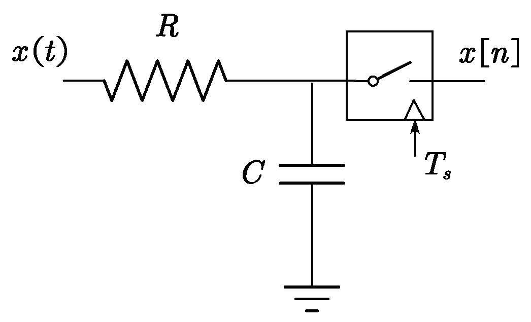
The S/H circuit is usually modeled by a first-order RC filter which is illustrated in Figure 1 [18,38]. The circuit is essentially a low-pass filter with the $-3$ dB bandwidth ${\Omega }_c=1/RC$. (“R” is the equivalent resistance of the circuit, and “C” is the equivalent capacitance.) In reality, the values for R and C differ between channels owing to variations in the manufacture, and they change slowly due to the fluctuation in temperature and voltage.

The transfer function of the m-th channel’s S/H circuit can be expressed as (1)

$$H_m\left(j\Omega \right)=\frac{1}{1+j\Omega \frac{1+{\beta }_m}{{\Omega }_c}},$$

(1)

where ${\beta }_m$ is the mismatch coefficient and ${\Omega }_c$ is the $-3$ dB bandwidth of the reference channel.

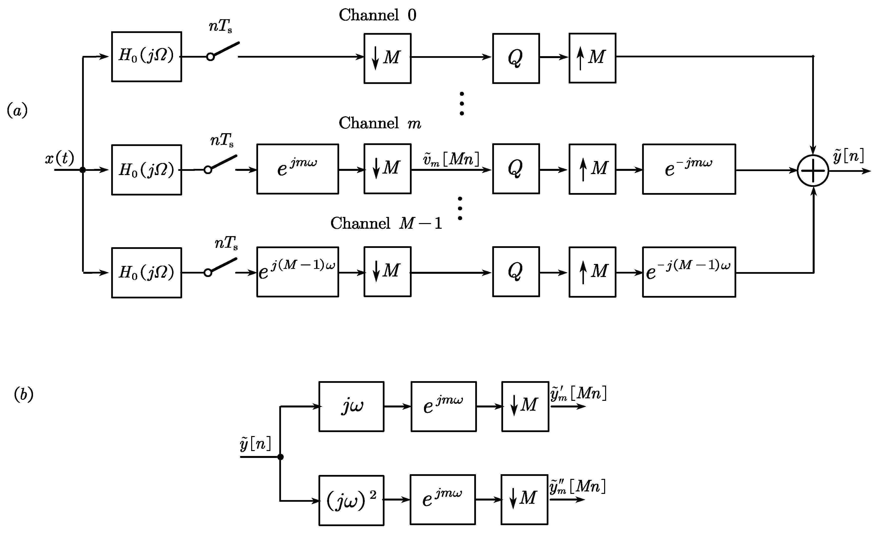
The M-channel TIADC’s model can be described as Figure 2.

To investigate the influence which bandwidth mismatch has on the dynamic performance of the TIADC, the discrete-time Fourier transform (DTFT) of downsampled signals $v_m[Mn]$ (defined in Figure 2) are

$$V_m\left(e^{jM\omega }\right)=\frac{1}{M}\sum _{k=0}^{M-1}{H}_m\left(e^{j\left(\omega -\frac{2k\pi }{M}\right)}\right)e^{j\left(\omega -\frac{2k\pi }{M}\right)}X\left(e^{j\left(\omega -\frac{2k\pi }{M}\right)}\right),$$

(2)

where

$$H_m(e^{j\omega })=H_m(j\Omega T_s),-\pi <\omega <\pi ,$$

(3)

and $X\left(e^{j\omega }\right)$ is the DTFT of signal $x[n]$. Then the DTFT of the TIADC’s output signal is

$$\begin{array}{c}\hfill Y\left(e^{j\omega }\right)=\sum _{m=0}^{M-1}{Y}_m\left(e^{j\omega }\right)=\sum _{m=0}^{M-1}{V}_m\left(e^{jM\omega }\right)e^{-jm\omega },\end{array}$$

(4)

where $Y_m\left(e^{j\omega }\right)$ is the DTFT of $y_m[n]$ defined in Figure 2.

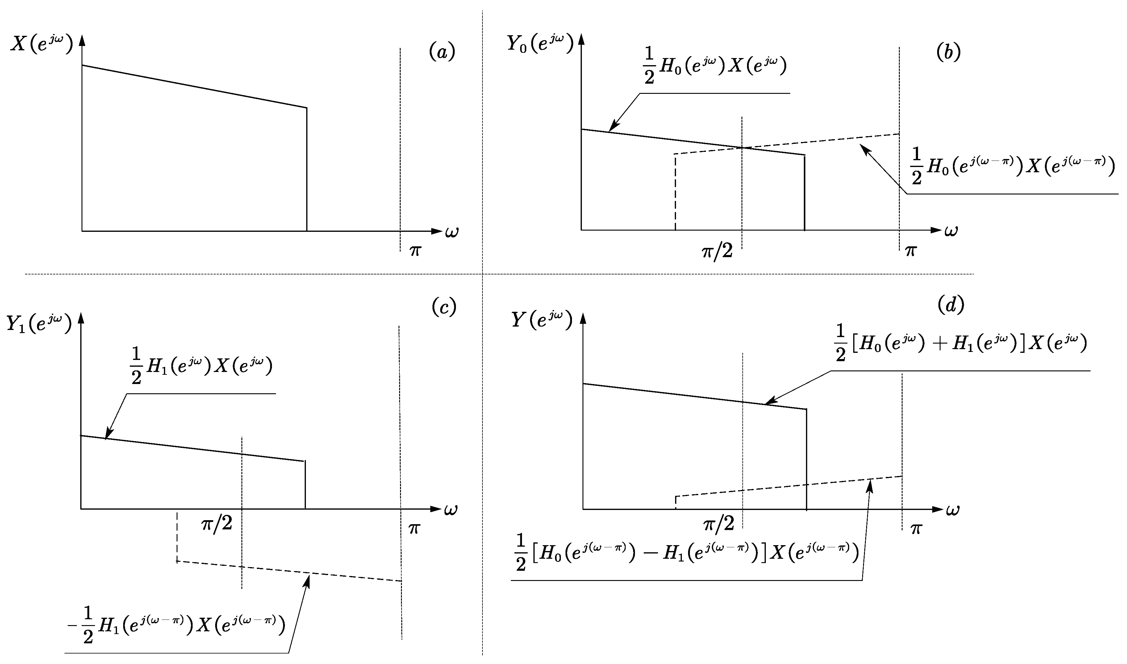
Taking 2-channel TIADC for instance, (4) is reduced to

$$\begin{array}{cc}\hfill Y\left(e^{j\omega }\right)& =Y_0\left(e^{j\omega }\right)+Y_1\left(e^{j\omega }\right)=V_0\left(e^{j2\omega }\right)+V_1\left(e^{j2\omega }\right)e^{-j\omega }\hfill \\ & =\frac{1}{2}\left[H_0\left(e^{j\omega }\right)+H_1\left(e^{j\omega }\right)\right]X\left(e^{j\omega }\right)+\frac{1}{2}\left[H_0\left(e^{j\left(\omega -\pi \right)}\right)-H_1\left(e^{j\left(\omega -\pi \right)}\right)\right]X\left(e^{j\left(\omega -\pi \right)}\right),\hfill \end{array}$$

(5)

where the first term is the linear distortion of the input spectrum, and the second term is the error spectrum. The two spectra are symmetric around frequency $\pi /2$, which is shown in Figure 3.

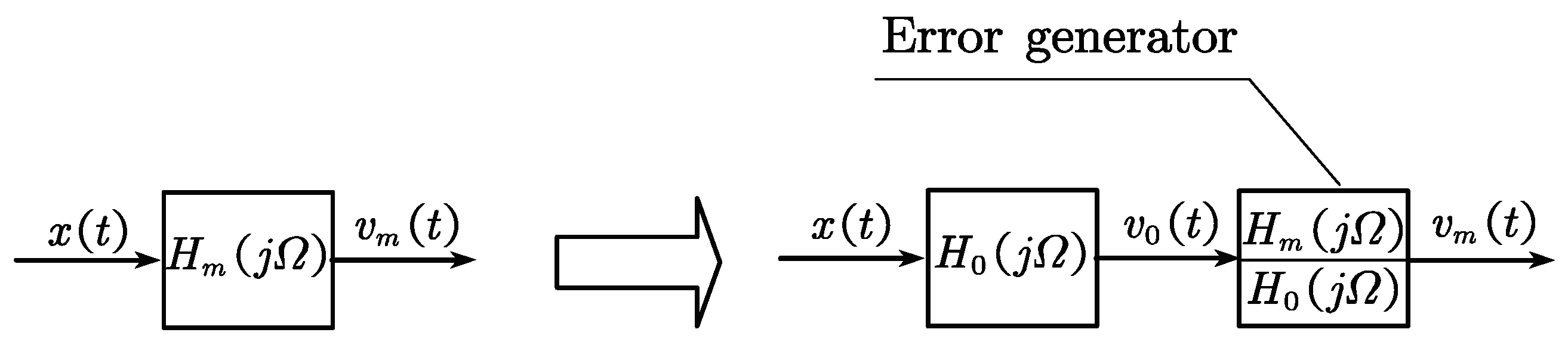
Like in a single ADC, there’s no need to explicitly equalize the frequency response, and it is not obligatory here for a TIADC [21,22]. So Channel 0 can be chosen as the reference channel (${\beta }_0=0$), and the filter $H_m(j\Omega )$ ($m\ne 0$) can be divided into two cascaded filters as is depicted in Figure 4. The bandwidth mismatch error can be regarded as the effect of an error generator whose transfer function is $H_m\left(j\Omega \right)/H_0\left(j\Omega \right)$.

To simplify the compensation, we try to use polynomials to approximate the transfer function of the error generator. Then the transfer function can be expressed in 2-order Taylor series as [39]

$$\frac{H_m\left(j\Omega \right)}{H_0\left(j\Omega \right)}=\frac{1+j\Omega \frac{1}{{\Omega }_c}}{1+j\Omega \frac{1+{\beta }_m}{{\Omega }_c}}\approx 1-j\Omega \frac{{\beta }_m}{{\Omega }_c}+{\left(j\Omega \right)}^2\frac{{\beta }_m\left(1+{\beta }_m\right)}{{\Omega }_c^2},$$

(6)

where $j\Omega$ is the frequency response of a differentiator. Usually, the bandwidth mismatch is small enough that 2-order Taylor series are sufficient to approximate the transfer function [21,22,29].(When the mismatch is larger, higher-order terms of Taylor series are needed. For example, in [22] where ${\Omega }_c=4\pi f_s$ and ${\beta }_m$ is around ${10}^{-3}$, the third order terms of Taylor series is needed.)

Then $v_m[Mn]$ (defined in Figure 2) can be expressed as (7)

$$\begin{array}{c}\hfill v_m\left[Mn\right]\approx {\tilde{v}}_m\left[Mn\right]-\frac{{\beta }_m}{{\omega }_c}{\tilde{y}}_m^{{}^{\prime }}\left[Mn\right]+\frac{{\beta }_m\left(1+{\beta }_m\right)}{{\omega }_c^2}{\tilde{y}}_m^{{}^{″}}\left[Mn\right]={\tilde{v}}_m\left[Mn\right]+e_m\left[Mn\right].\end{array}$$

(7)

The meanings of ${\tilde{v}}_m\left[Mn\right]$, ${\tilde{y}}_m^{{}^{\prime }}\left[Mn\right]$ and ${\tilde{y}}_m^{{}^{″}}\left[Mn\right]$ are given in Figure 5. Now our task is to cancel the error by identifying the mismatch coefficient ${\beta }_m$ and approximating the error $e_m[Mn]$.

3. Mismatch Compensation

Since the compensation structure is utilized in the identification, the compensation is firstly considered. When the mismatch coefficient ${\widehat{\beta }}_m$ is identified (which is described in detail in Section 4), the error $e_m[Mn]$ in (7) can be generated in theory. In practice, however, no prior knowledge about the desirable signal $\tilde{y}\left[n\right]$ (defined in Figure 5) is available. One widely acceptable solution is to approximate it by $y\left[n\right]$ [6,7,22,28].

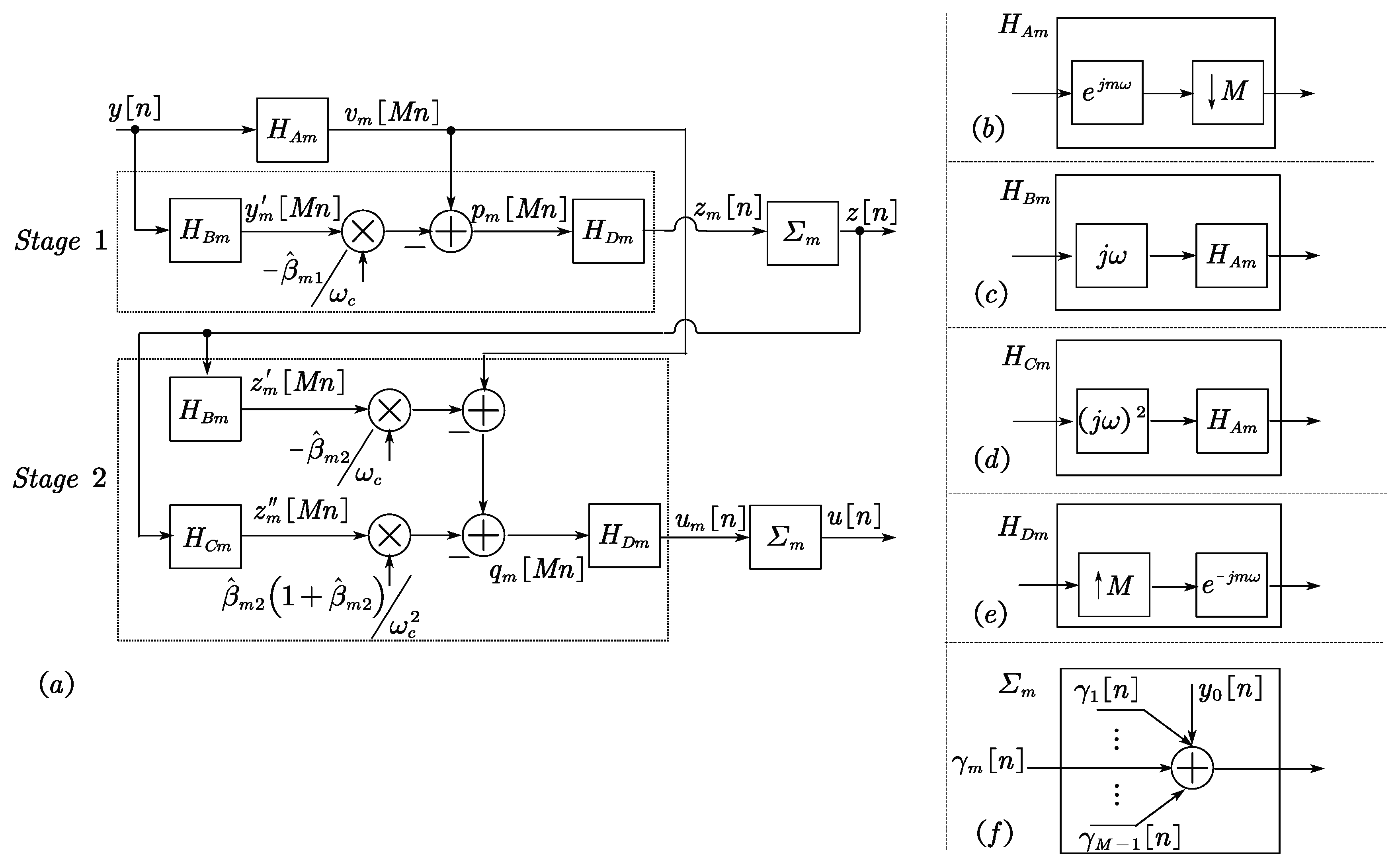
The Richardson iteration structure illuminated in Figure 6 is introduced for high precision compensation [40]. In Stage 1, we try to generate the 1st-order term of Taylor series in (7) using the output signal $y\left[n\right]$ and then eliminate it from the original output signal. Then the compensated down-sampled signal of Channel m is

$$\begin{array}{cc}\hfill p_m\left[Mn\right]& =v_m\left[Mn\right]+\frac{{\widehat{\beta }}_{m1}}{{\Omega }_c}{y}_m^{{}^{\prime }}\left[Mn\right]\hfill \\ & ={\tilde{v}}_m\left[Mn\right]+\frac{{\widehat{\beta }}_{m1}-{\beta }_m}{{\Omega }_c}{\tilde{y}}_m^{{}^{\prime }}\left[Mn\right]+\frac{{\beta }_m\left(1+{\beta }_m-{\widehat{\beta }}_{m1}\right)}{{\Omega }_c^2}{\tilde{y}}_m^{{}^{″}}\left[Mn\right]+o\left({\tilde{y}}_m^{{}^{″}}\left[Mn\right]\right),\hfill \end{array}$$

(8)

where ${\widehat{\beta }}_{m1}$ is the identified coefficient for ${\beta }_m$ in Stage 1, and $o\left({\tilde{y}}_m^{{}^{″}}\left[Mn\right]\right)$ is higher order differential of ${\tilde{y}}_m\left[Mn\right]$ which is too weak to consider. Comparing (8) with (7), $p_m\left[Mn\right]$ is closer to ${\tilde{v}}_m\left[Mn\right]$ than $v_m\left[Mn\right]$, where the detailed derivation is given in [22,40]. Such being the case, we can use $p_m\left[Mn\right]$ instead of $v_m\left[Mn\right]$ for further approximation to ${\tilde{v}}_m\left[Mn\right]$ in the error cancellation of Stage 2.

In Stage 2, we try to approximate the 1st- and 2nd-order terms of Taylor series in (7). Note that the generated error should be subtracted from the original signal $v_m\left[Mn\right]$ to further suppress the distortion. Then the compensated down-sampled signal of Channel m is denoted as

$$\begin{array}{c}{q}_m\left[Mn\right]=v_m\left[Mn\right]+\frac{{\widehat{\beta }}_{m2}}{{\Omega }_c}{z}_m^{{}^{\prime }}\left[Mn\right]-\frac{{\widehat{\beta }}_{m2}\left(1+{\widehat{\beta }}_{m2}\right)}{{\Omega }_c^2}{z}_m^{{}^{″}}\left[Mn\right]\hfill \\ ={\tilde{v}}_m\left[Mn\right]+\frac{{\widehat{\beta }}_{m2}-{\beta }_m}{{\Omega }_c}{\tilde{y}}_m^{{}^{\prime }}\left[Mn\right]+\frac{\left(1+{\beta }_m-{\widehat{\beta }}_{m1}\right)\left({\beta }_m-{\widehat{\beta }}_{m2}\right)-{\widehat{\beta }}_{m2}^2}{{\Omega }_c^2}{\tilde{y}}_m^{{}^{″}}\left[Mn\right]+o\left({\tilde{y}}_m^{{}^{″}}\left[Mn\right]\right),\hfill \end{array}$$

(9)

where ${\widehat{\beta }}_{m2}$ is the identified coefficient for ${\beta }_m$ in Stage 2. The error is further suppressed in Stage 2 compared with Stage 1.

More stages are needed if the mismatch is larger or higher precision is required. For instance, in Stage 3, the 1st-, 2nd-, and 3rd-order terms of the Taylor’s series can be approximated using $u[n]$, and are then subtracted from $y[n]$ to get a signal closer to the expected one.

4. Coefficient Identification

The coefficient identification is based on the statistical properties of the input signals. Most real-life signals are WSS and modulo M quasi-stationary, whose definitions are given below [3,5].

Definition 1.

Wide-Sense Stationary

A discrete-time signal $u[k]$ is said to be WSS if its 1st and 2nd moments are time-invariant. That is

$$m_u=\underset{N\to \infty }{\lim }\frac{1}{N}\sum _{k=1}^{N}E\left(u\left[k\right]\right),$$

(10)

and

$$R_u\left[n\right]=\underset{N\to \infty }{\lim }\frac{1}{N}\sum _{k=1}^{N}E\left(u\left[k+n\right]u\left[k\right]\right),$$

(11)

where $E(·)$ is the expectation.

Definition 2.

Modulo M Quasi-Stationary

Assume

$${\overline{f}}_{u_{i_1},u_{i_2},\cdots }=\underset{N\to \infty }{\lim }\frac{1}{N}\sum _{t=1}^{N}f\left(u_{i_1}\left[t\right],u_{i_2}\left[t\right],\cdots \right),i_1,i_2,\cdots =0,1,\cdots ,M-1$$

(12)

exists for a function $f(·,·,\cdots )$. Then u is modulo M quasi-stationary with respect to f if

$${\overline{f}}_{i_1,i_2,\cdots }={\overline{f}}_{\left\{\left(i_1+l\right)\mathrm{mod}M,\left(i_2+l\right)\mathrm{mod}M,\cdots \right\}},l\in Z.$$

(13)

(“mod” is the remainder operator, and “Z” is the set of integers.) The modulo M quasi-stationary property guarantees that the input signal manifests the same statistical properties for all channels in the time-interleaved system.

Assume $x[n]$ is WSS and modulo M quasi-stationary with respect to the function $f(x_i,x_{i-1})={(x_i-x_{i-1})}^2$. Then the down-sampled signal for Channel m is denoted as

$$v_m\left[Mn\right]=A_{m}x\left(Mn{T}_s+t_m\right),m=0,1,2,\cdots ,M-1,$$

(14)

where

$$A_m=\frac{1}{\sqrt{1+{\left(\frac{\left(1+{\beta }_m\right)\omega }{{\Omega }_c}\right)}^2}}$$

(15)

is the magnitude response of the filter $H_m(e^{j\omega })$, and

$$t_m=-\frac{1}{\omega }\arctan \left(\frac{\left(1+{\beta }_m\right)\omega }{{\Omega }_c}\right),s.t.t_m\in \left(-\frac{\pi }{2},\frac{\pi }{2}\right)$$

(16)

is the phase response of the filter $H_m(e^{j\omega })$.

Then the mean squared difference between the down-sampled signals of adjacent channels is

$$\begin{array}{cc}\hfill D_{v_m,v_{m-1+\left|\lfloor \frac{m-1}{M}\rfloor \right|·M}}=& \underset{N\to \infty }{\lim }\frac{1}{N}\sum _{n=1}^N{\left(v_m\left[Mn\right]-v_{m-1+\left|\lfloor \frac{m-1}{M}\rfloor \right|·M}\left[M\left(n+\lfloor \frac{m-1}{M}\rfloor \right)\right]\right)}^2\hfill \\ \hfill =& \left(A_m+A_{m-1+\left|\lfloor \frac{m-1}{M}\rfloor \right|·M}\right){\sigma }^2-2A_m{A}_{m-1+\left|\lfloor \frac{m-1}{M}\rfloor \right|·M}{R}_x\left(T_s+t_m-t_{m-1+\left|\lfloor \frac{m-1}{M}\rfloor \right|M}\right),\hfill \\ & m=0,1,\cdots ,M-1,\hfill \end{array}$$

(17)

where $\lfloor ·\rfloor$ is the floor operator, and $|·|$ is the absolution operator. In (17), ${\sigma }^2$ stands for the variance of the signal $x[n]$

$${\sigma }^2=\underset{N\to \infty }{\lim }\frac{1}{N}\sum _{n=0}^N{x}^2\left[n\right],$$

(18)

and $R_x(·)$ means the autocorrelation of the signal $x[n]$

$$R_x\left(\tau \right)=\underset{N\to \infty }{\lim }\frac{1}{N}\sum _{n=0}^{N}x\left[n\right]x\left[n+\tau \right].$$

(19)

When $m>1$, (17) becomes

$$D_{v_m,v_{m-1}}=\underset{N\to \infty }{\lim }\frac{1}{N}\sum _{n=1}^N{\left(v_m\left[Mn\right]-v_{m-1}\left[Mn\right]\right)}^2,m=1,\cdots ,M-1.$$

(20)

When $m=0$, (17) becomes

$$D_{v_0,v_{M-1}}=\underset{N\to \infty }{\lim }\frac{1}{N}\sum _{n=1}^N{\left(v_0\left[Mn\right]-v_{M-1}\left[M\left(n-1\right)\right]\right)}^2.$$

(21)

The value of (17) varies with the bandwidth mismatch ${\beta }_m$.

LMS algorithm is adopted to estimate ${\beta }_m$. By considering all the distinctions between the mean squared differences indicated by (17), the loss function can be established as

$$P=\sum _{i=1}^{M-1}\sum _{j=0}^{i-1}{\left(D_{v_i,v_{i-1+\left|\lfloor \frac{i-1}{M}\rfloor \right|·M}}-D_{v_j,v_{j-1+\left|\lfloor \frac{j-1}{M}\rfloor \right|·M}}\right)}^2.$$

(22)

Only when all ${\beta }_m=0$, the cost function $P=0$.

In Stage 1, the identified coefficient ${\widehat{\beta }}_1$ is searched as the following four steps.

Step 1: Calculate the mean squared differences between adjacent channels’ compensated signals as (In practice, the limit expressed in (17) cannot be realized, and it is approximated by a batch of finite samples instead [3,5].)

$$D_{p_i,p_{i-1+\left|\lfloor \frac{i-1}{M}\rfloor \right|·M}}=\frac{1}{N}\sum _{n=1}^N{\left(p_i\left[Mn\right]-p_{i-1+\left|\lfloor \frac{i-1}{M}\rfloor \right|·M}\left[M·\left(n+\lfloor \frac{i-1}{M}\rfloor \right)\right]\right)}^2,$$

(23)

where $p_0[Mn]=v_0[Mn]$.

Step 2: Calculate the cost function as

$$P=\sum _{i=1}^{M-1}\sum _{j=0}^{i-1}{\left(D_{p_i,p_{i-1+\left|\lfloor \frac{i-1}{M}\rfloor \right|·M}}-D_{p_j,p_{j-1+\left|\lfloor \frac{j-1}{M}\rfloor \right|·M}}\right)}^2,$$

(24)

which is also shown in Figure 7.

Step 3: Calculate the partial differential of ${\widehat{\beta }}_{m1}$ as

$$\begin{array}{cc}\hfill \frac{\partial P\left(k\right)}{\partial {\widehat{\beta }}_{m1}\left(k\right)}=& 2\sum _{i=m+2}^{M-1}\sum _{j=m}^{i-1}\left(D_{p_i,p_{i-1}}-D_{p_j,p_{j-1}}\right)\left(-\frac{\partial D_{p_j,p_{j-1}}}{\partial {\widehat{\beta }}_{m1}\left(k\right)}\right)\hfill \\ & +2\sum _{i=m}^{m+1}\sum _{j=0}^{m-1}\left(D_{p_i,p_{i-1}}-D_{p_j,p_{j-1+\left|\lfloor \frac{i-1}{M}\rfloor \right|·M}}\right)·\frac{\partial D_{p_i,p_{i-1}}}{\partial {\widehat{\beta }}_{m1}\left(k\right)}\hfill \\ & +2\left(D_{p_{m+1},p_m}-D_{p_m,p_{m-1}}\right)·\left(\frac{\partial D_{p_{m+1},p_m}}{\partial {\widehat{\beta }}_{m1}\left(k\right)}-\frac{\partial D_{p_m,p_{m-1}}}{\partial {\widehat{\beta }}_{m1}\left(k\right)}\right)\hfill \end{array},$$

(25)

$$\frac{\partial D_{p_{m+1},p_m}}{\partial {\widehat{\beta }}_{m1}\left(k\right)}=\frac{2}{N}\sum _{n=1}^N\left(p_{m+1}\left[Mn\right]-p_m\left[Mn\right]\right)·\left(-\frac{\partial p_m}{\partial {\widehat{\beta }}_{m1}\left(k\right)}\right),$$

(26)

$$\frac{\partial D_{p_m,p_{m-1}}}{\partial {\widehat{\beta }}_{m1}\left(k\right)}=\frac{2}{N}\sum _{n=1}^N\left(p_m\left[Mn\right]-p_{m-1}\left[Mn\right]\right)·\frac{\partial p_m}{\partial {\widehat{\beta }}_{m1}\left(k\right)},$$

(27)

$$\frac{\partial p_m}{\partial {\widehat{\beta }}_{m1}\left(k\right)}=\frac{y_m^{{}^{\prime }}\left[Mn\right]}{{\Omega }_c},$$

(28)

where k means the k-th searching loop and $m=1,2,\cdots ,M-1$.

Step 4: Update the coefficients as

$${\widehat{\beta }}_{m1}\left(k+1\right)={\widehat{\beta }}_{m1}\left(k\right)-\mu \frac{dP\left(k\right)}{d{\widehat{\beta }}_{m1}\left(k\right)},$$

(29)

where $\mu$ is the searching step.

In Stage 2, the identification procedure is similar to the above four steps except that $q_m[Mn]$ is used instead of $p_m[Mn]$. The partial derivative $\partial q_m\left[Mn\right]/\partial {\widehat{\beta }}_{m2}\left(k\right)$ used in Step 3 is

$$\frac{\partial q_m\left[Mn\right]}{\partial {\widehat{\beta }}_{m2}\left(k\right)}=\frac{z_m^{{}^{\prime }}\left[Mn\right]}{{\Omega }_c}-\frac{\left(2{\widehat{\beta }}_{m2}\left(k\right)+1\right)z_m^{{}^{″}}\left[Mn\right]}{{\Omega }_c^2}.$$

(30)

Moreover, it should be noted that before the identification, notch filters with notch frequencies at $m·f_s/(2M)$ are needed to exclude the error caused by coherent sampling, where $m=1,2,\cdots ,M-1$.

5. Simulation and Comparison

A quantizer of 14 bits is utilized in the simulations below. The filters are designed by “firpm” function in MATLAB^©, which uses the Parks-McClellan optimal equiripple design algorithm. The $-3$ dB bandwidth of Channel 0 is ${\Omega }_c=6\pi f_s$. We define a term for sinusoidal signals to indicate the dynamic performance of the TIADC: the Largest-Signal-to-largest-Spurious-component-Ratio (LSSR).

$$\mathrm{LSSR}\left(\mathrm{dBc}\right)=10{\log }_{10}\frac{\max \left(P_{signal,i}\right)}{\max \left(P_{spurious,j}\right)},$$

(31)

where $P_{signal,i}$ is the power of the i-th sinusoidal component in the DFT spectrum, and $P_{spurious,j}$ is the power of the j-th spurious component including harmonic component. For a single-tone sinusoid, the LSSR is equal to the spurious-free dynamic range (SFDR).

5.1. Effectiveness

We evaluate the effectiveness of the proposed approach by simulating two cases.

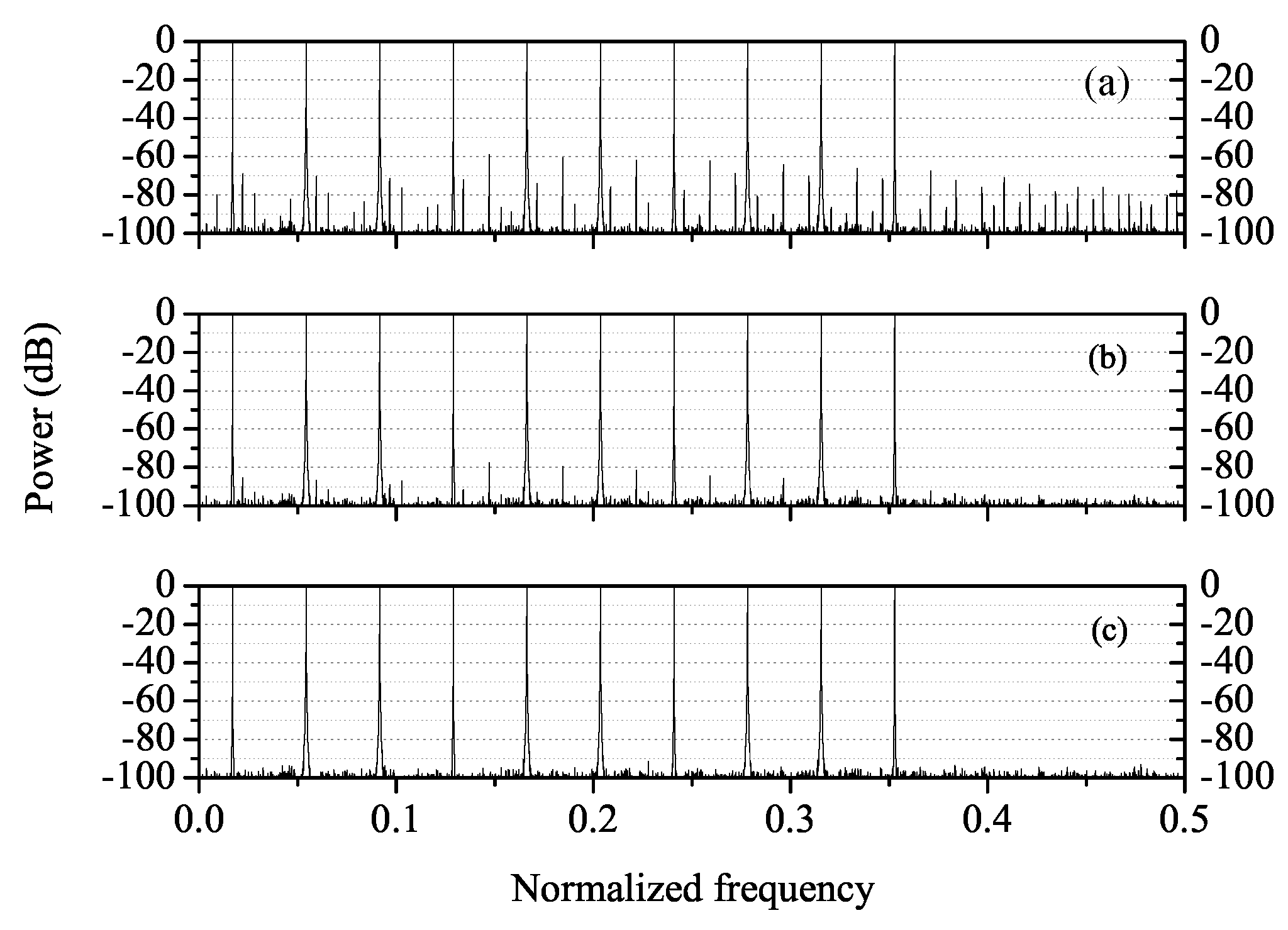
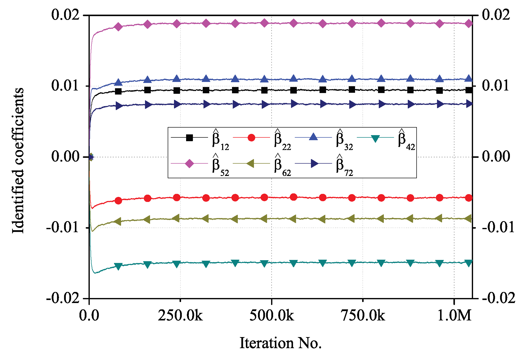
In the first case, an 8-channel TIADC is simulated. The parameters are set as

Table 1. Simulation parameters.

Frequency Range	Signal Type	Batch Size	Differentiator Order
$0\sim 0.4f_s$	10-tone sinusoid	$N=512$	$N_d=20$

and

Table 2. Mismatch coefficients.

${\mathit{\beta }}_{\mathbf{1}}$	${\mathit{\beta }}_{\mathbf{2}}$	${\mathit{\beta }}_{\mathbf{3}}$	${\mathit{\beta }}_{\mathbf{4}}$	${\mathit{\beta }}_{\mathbf{5}}$	${\mathit{\beta }}_{\mathbf{6}}$	${\mathit{\beta }}_{\mathbf{7}}$
$0.01$	$-0.005$	$0.012$	$-0.014$	$0.02$	$-0.008$	$0.008$

. The output power spectra are demonstrated in Figure 8. The higher vertical lines up to 0 dB stand for the desirable input signals, while the lower vertical lines are the bandwidth mismatch induced errors which should be suppressed below the noise floor. The signal-to-noise-and-distortion (SINAD) is 62.15 dB and the LSSR is 59.07 dBc before calibration, while they are enhanced to 74.95 dB and 77.53 dBc after Stage 1 calibration, and then to 75.78 dB and 91.39 dBc after Stage 2 calibration. The identified coefficients in Stage 2 calibration plotted in Figure 9 and those in Table 2 are close but not identical, because we use $y[n]$ and $z[n]$ to approximate the error rather than $\tilde{y}[n]$ in (8) and (9). Therefore, the algorithm proposed in this paper can accurately identify the mismatch coefficients without much prior information of the input signal other than its WSS and modulo 8 quasi-stationary properties.

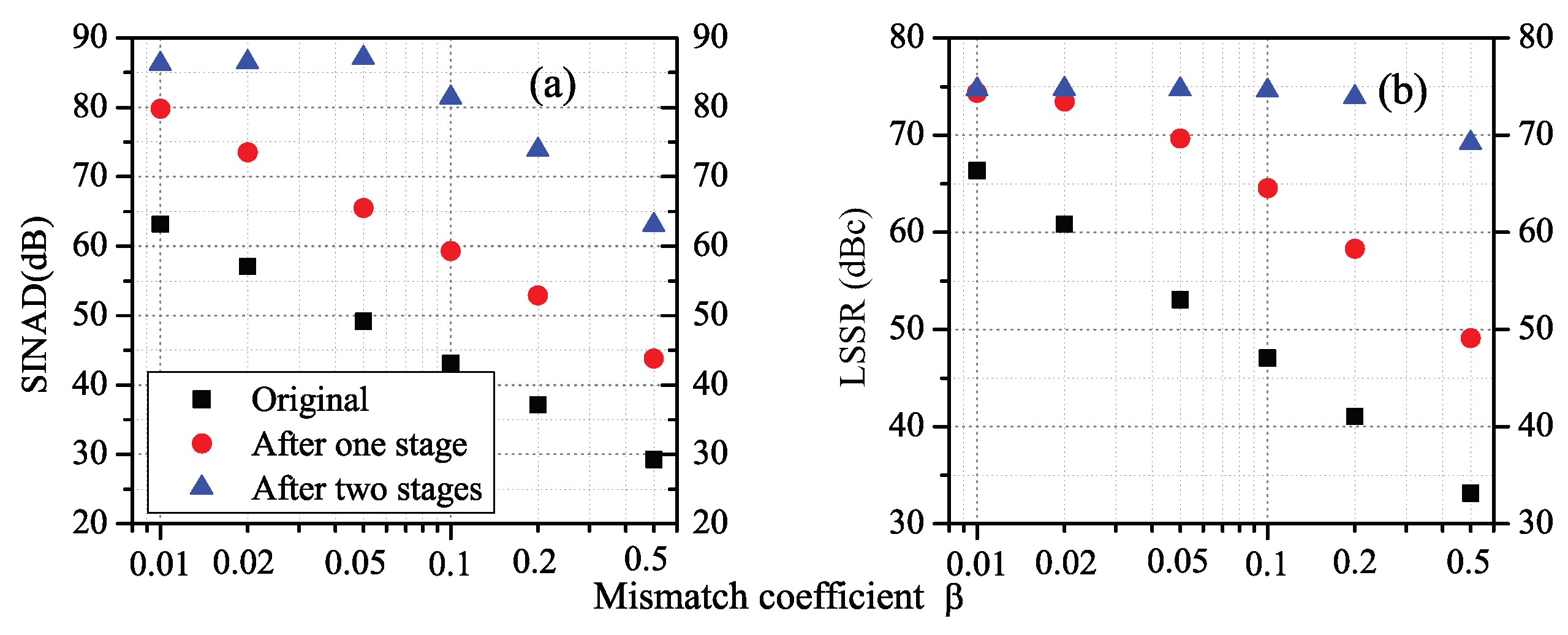
In the second case, the performance enhancement for different mismatch coefficients in a 2-channel TIADC is illustrated. Parameters are set as

Table 3. Simulation parameters.

Frequency Range	Signal Type	Batch Size	Differentiator Order
$0\sim 0.45f_s$	10-tone sinusoids	$N=$ 16,384	$N_d=60$

. The performance before and after calibration are depicted in Figure 10, showing that our algorithm works well under circumstances of different mismatch levels. Theoretically, larger promotion should have been achieved at smaller mismatch circumstance where the error in the compensation resulted from approximating y or z to $\tilde{y}$ is smaller (ref. (8) and (9)). Whereas actually in Figure 10, the SINAD and the LSSR initially increase with the decreasing mismatch and then saturate at certain values. This is because the quantization bits of the TIADC limit the further improvement. By increasing the quantization bits, a higher promotion can be achieved, and the SINAD and LSSR will saturate at larger values.

In this subsection, the calibration method performs well for an 8-channel TIADC and a 2-channel TIADC with different mismatch coefficients.

5.2. Parameter Selection

We show the differentiator order selection and the batch size selection by simulating two cases. A 2-channel TIADC with the mismatch coefficient $\beta =0.2$ is used for these two cases.

In the first case, the effect which the differentiator order has on the algorithm performance is surveyed. Simulation parameters except the differentiator order are set as Table 3. The results are depicted in Figure 11. One can achieve better SINAD and LSSR along with higher differentiator’s order. A 40-order differentiator is enough when the mismatch coefficient is below 0.2 and input spectrum occupies the lower $90\%$ fraction of the Nyquist band. Moreover, the differentiator’s order also has a connection with its pass-band (PB) width. For example, a 20-order differentiator is enough if the input signal only occupies the lower $80\%$ fraction of the Nyquist band.

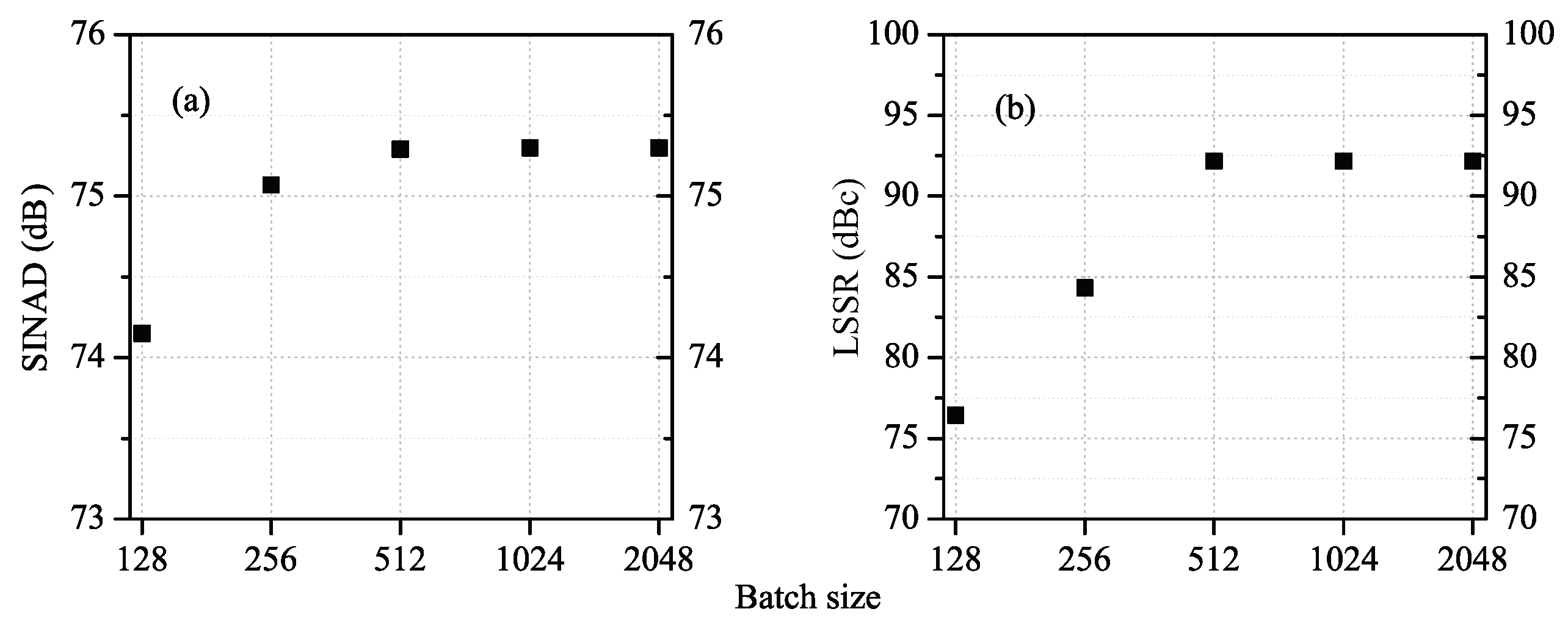
In the second case, the effect which the batch size for coefficient identification has on the calibration precision is surveyed. The input signal is set as Table 3, and the differentiator order is set as 40. The results are depicted in Figure 12. One can achieve better SINAD and LSSR along with larger batch size for identification, because the cost function is established under the circumstance where $N\to \infty$ as (17). However, the resource consumption also increases with the batch size. Batch size of 512 is moderate for both dynamic performance and resource consumption.

In this subsection, we show the connection between the calibration precision and the differentiator order or the batch size. Eventually, differentiator order of 20 and batch size of 512 are selected for moderate dynamic performance and resource consumption.

5.3. Comparisons

In this section, we choose the IFB-based method [23,35] and the I/Q-based method [24,25] for comparison which are better than other methods both in bandwidth efficiency and complexity. A 2-channel TIADC is used for the following two cases.

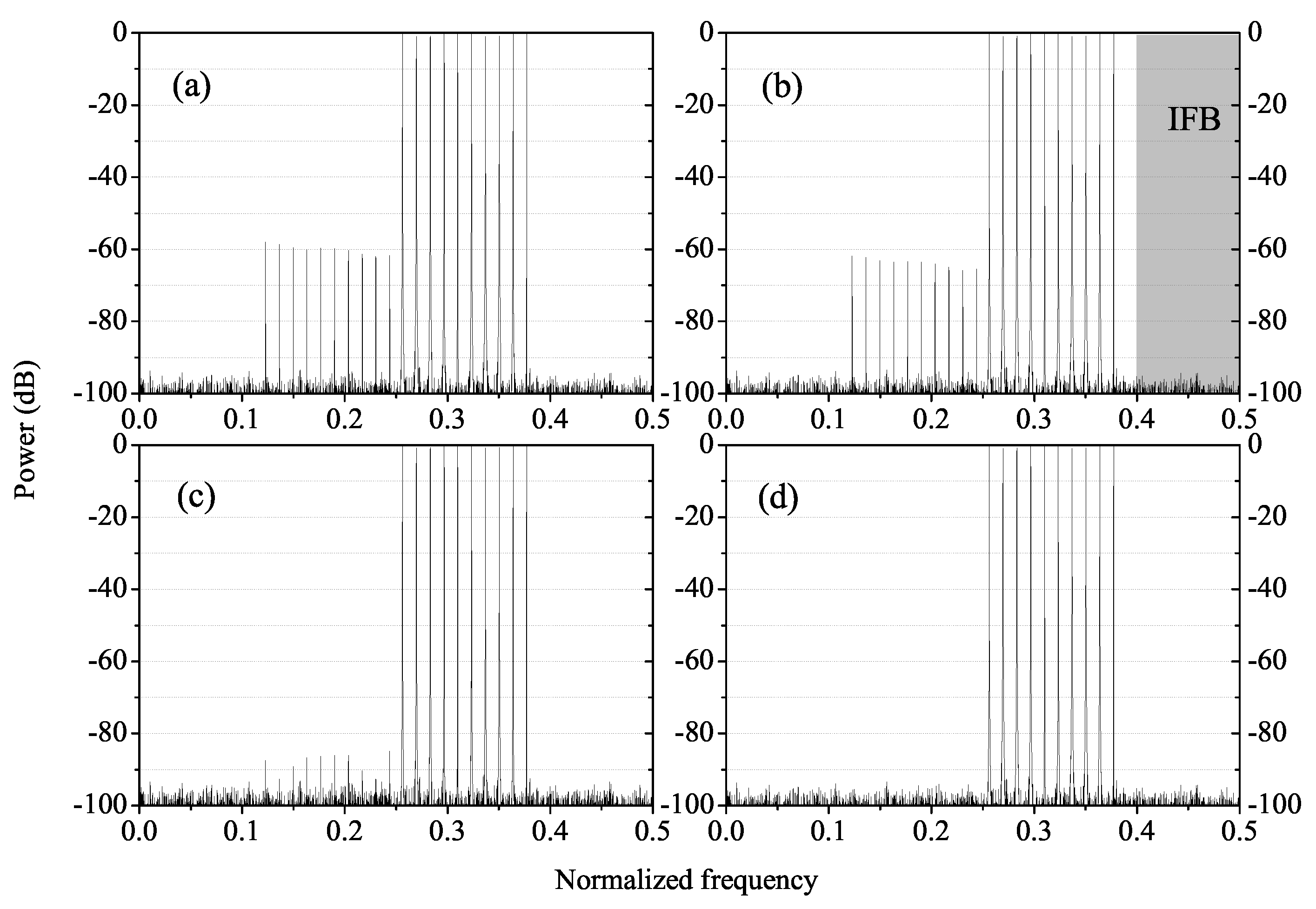
In the first case, the LSSR improvements of the three methods are compared. The parameters are set as

Table 4. Common simulation parameters for LSSR improvement comparison.

Frequency Range	Signal Type	Mismatch Coefficient
$0.26\sim 0.38f_s$	10-tone sinusoids	$\beta =0.02$

,

Table 5. Simulation parameters for the high-pass filter in the input-free band (IFB) method.

Order	PB Cut-Off Frequency	SB Cut-Off Frequency	PB Attenuation	SB Attenuation
$N_{hp}=40$	$0.495f_s$	$0.4f_s$	$-1$ dB	$-115$ dB

Note: (1) “PB” is the abbreviation for pass-band. (2) “SB” is the abbreviation for stop-band.

,

Table 6. Simulation parameters for the I/Q method.

Hilbert Filter Order	Hilbert Filter PB	Compensation Filter Order
$N_{hb}=10$	$0.075f_s\sim 0.425f_s$	$N_{cp}=2$

and

Table 7. Simulation parameters for the proposed method.

Batch Size	Differentiator Order
$N=512$	$N_d=20$

, and the differentiators used in the IFB method and our method are identical. The output power spectra are demonstrated in Figure 13. The SINAD is 59.39 dB and the LSSR is 58.00 dBc before calibration, and they are slightly enhanced to 62.89 dB and 61.77 dBc using the IFB-based method, and they are enhanced to 75.08 dB and 84.95 dBc using the I/Q-based method, and they are enhanced to 77.34 dB and 93.05 dBc employing the method proposed in this paper.

For the IFB-based method, an input-free band is created in the frequency spectrum by oversampling where the mismatch-induced error exists without input signal. By exerting a high-pass filter whose passband coincides with the IFB, the mismatch coefficients can be identified. However, in this case, the error spectrum does not appear in the IFB and the identification fails (ref. Figure 13b). For some other kinds of narrow-band signals, the IFB-based method cannot also work.

For the I/Q-based method, the TIADC’s output signal is converted to a complex signal with frequency shift, which is similar to the homodyne receiver’s output signal with I/Q mismatch, and the I/Q mismatch calibration technique is used to calibrate the TIADC’s mismatch. The compensation filter’s coefficients are determined by restoring the complex signal’s circularity. However, in this case where the signals are multi-tone sinusoids, there is no remarkable difference between the circularity of the signal without mismatch and that of the signal with mismatch, and therefore the calibration cannot suppress the error to the noise floor. For some other types of signals mainly composed of sinusoids, the I/Q-based method also cannot work. So compared with the other two methods, our method has more extensive applicability for different types of signals.

In the second case, the resource consumptions are compared among the three methods when the same error attenuation is achieved after calibration. The multiplications used in one loop of calibration is chosen as the indicator. The input signal is set as

Table 8. Input signal for resource consumption comparison.

Signal Type	Carrier Frequency	Duration/Sample
16-QAM	$0.05f_s$	10

so that all the methods can work effectively. $\beta =0.08$. The variables $N_d$, $N_{hp}$, $N_{cp}$, $N_{hb}$ and N are defined in Table 1, Table 5 and Table 6.

The resource consumption for the I/Q-based method is calculated as follows. $\langle 1\rangle$ It needs $0.5N_{hb}$ multiplications to pass the output signal through the Hilbert filter because the filter’s taps are anti-symmetric with a null center tap. $\langle 2\rangle$ It needs $4(N_{cp}+1)$ multiplications to compensate the signal, since both the signal and the filter taps are complex, and multiplying two complex numbers actually needs four multiplications of real numbers. $\langle 3\rangle$ It consumes $4(N_{cp}+1)$ multiplications to update the compensation filter’s taps. Adding $\langle 1\rangle$ to $\langle 3\rangle$, the total number of multiplications needed in one calibration iteration is

$$8N_{cp}+0.5N_{hb}+8.$$

(32)

Here, $N_{hb}=10$ and $N_{cp}$ is set to be 0, which results in 13 multiplications in total.

The IFB-based method and the proposed method use the common compensation technique and the consumption is calculated as follows. For simplicity, only the first Richardson iteration is considered for both the IFB method and ours. $\langle 4\rangle$ It needs $0.5N_d$ multiplications to get $v^{{}^{\prime }}[2n]$ because the differentiator’s taps are anti-symmetric with a null center tap. $\langle 5\rangle$ It requires 1 multiplication to scale $v^{{}^{\prime }}[2n]$ with estimated coefficients as (8).

The consumption of the identification procedure for the IFB-based method is calculated as follows. $\langle 6\rangle$ It consumes $(0.5N_h+1)$ multiplications to filter $z[n]$ due to the anti-symmetric property of the high-pass filters’ taps. $\langle 7\rangle$ It requires 2 multiplications to update ${\widehat{\beta }}_1$. Adding $\langle 4\rangle$ to $\langle 7\rangle$, the total number of multiplications needed in one calibration loop is

$$0.5\left(N_d+N_{hp}\right)+3.$$

(33)

Here, $N_d=20$ and $N_{hp}=40$, which results in 33 multiplications in total.

The consumption of the identification procedure for the proposed method is calculated as follows. $\langle 8\rangle$ It takes $2N$ multiplications to calculate $D_{v_1,v_0}$ and $D_{v_0,v_1}$ as (17). $\langle 9\rangle$ It requires $(2N+1)$ multiplications to calculate $\partial P/\partial {\widehat{\beta }}_1$ as (25) to (28). $\langle 10\rangle$ It requires 1 multiplication to update ${\widehat{\beta }}_1$. (All the constant coefficients used in (17), and (25) to (28) can be combined together into the step $\mu$, so only one multiplication is needed to consider them all.) Adding $\langle 4\rangle$ to $\langle 5\rangle$ and $\langle 8\rangle$ to $\langle 10\rangle$, the total number of multiplications needed in one calibration loop is

$$4N+0.5N_d+2.$$

(34)

Here, $N_d=20$ and N is set to be 32, which results in 140 multiplications in total.

The comparison results of the above two cases are shown in

Table 9. Comparisons between the proposed method, the IFB-based method, and the I/Q based method.

Method	LSSR Improvement	Resource Consumption	Channel No.
This paper	35.05 dBc	141	M
IFB-based method [23,35]	3.77 dBc	42	2
I/Q-based method [24,25]	26.95 dBc	13	2 or 4

. The proposed method in this paper is more complex compared with the other two methods when calibrating the same signals, but this method can apply to more types of signals and more channels whereas the other two methods cannot.

6. Conclusions

This paper proposes a statistics-based calibration method for S/H mismatches in M-channel TIADCs. The mismatch coefficients are identified by eliminating the statistical differences between channels using the LMS algorithm. The mismatch-induced errors are approximated using multipliers and differentiators, and are eliminated from the original output samples afterwards. Although the complexity is higher compared with the IFB-based method and the I/Q-based method, the proposed algorithm in this paper has more extensive applicability for different signals and different numbers of channels.

There are three circumstances where our method should be given priority. When the signal’s bandwidth is unknown or is narrow to some extent, it is more reliable to use our method than the IFB-based method. When the signal’s components are unknown or the signal is mainly composed of sinusoids, our method can provide higher calibration precision than the I/Q-based method. When the number of channels is more than four, only our method can work.

To realize our method in a real-time way, a full-parallel structure can be employed in FPGAs. For instance in [30], fast FIR algorithm is used to parallelize the differentiators, which can make the FPGA’s low clock frequency more compatible with the TIADC’s high sampling rate and reduce the power consumption meanwhile. The batch size N can also be reduced since the accumulation in (23) can be shifted into the iteration process of (29) and (30) at the cost of more iterations. Furthermore, for the high sampling rate, the extra iterations do not bring much longer convergence time.

References

- Black, W.; Hodges, D. Time interleaved converter arrays. IEEE J. Solid-State Circuits 1980, 6, 1022–1029. [Google Scholar] [CrossRef]
- Jamal, S.M.; Fu, D.; Chang, N.; Hurst, P.J.; Lewis, S.H. A 10-b 120-Msample/s time-interleaved analog-to-digital converter with digital background calibration. IEEE J. Solid-State Circuits 2002, 12, 1618–1627. [Google Scholar] [CrossRef]
- Elbornsson, J.; Gustafsson, F.; Eklund, J.E. Blind adaptive equalization of mismatch errors in a time-interleaved A/D converter system. IEEE Trans. Circuits Syst. I Regul. Pap. 2003, 1, 151–158. [Google Scholar] [CrossRef]
- Jamal, S.M.; Fu, D.; Singh, M.P.; Hurst, P.J.; Lewis, S.H. Calibration of sample-time error in a two-channel time-interleaved analog-to-digital converter. IEEE Trans. Circuits Syst. I Regul. Pap. 2004, 1, 130–139. [Google Scholar] [CrossRef]
- Elbornsson, J.; Gustafsson, F.; Eklund, J.E. Blind equalization of time errors in a time-interleaved ADC system. IEEE Trans. Signal Process. 2005, 4, 1413–1424. [Google Scholar] [CrossRef]
- Chi, H.L.; Hurst, P.J.; Lewis, S.H. A Four-Channel Time-Interleaved ADC With Digital Calibration of Interchannel Timing and Memory Errors. IEEE J. Solid-State Circuits 2010, 10, 2091–2103. [Google Scholar] [CrossRef]
- Matsuno, J.; Yamaji, T.; Furuta, M.; Itakura, T. All-Digital Background Calibration Technique for Time-Interleaved ADC Using Pseudo Aliasing Signal. IEEE Trans. Circuits Syst. I Regul. Pap. 2013, 5, 1113–1121. [Google Scholar] [CrossRef]
- Li, D.; Zhu, Z.; Zhang, L.; Yang, Y. A background fast convergence algorithm for timing skew in time-interleaved ADCs. Microelectron. J. 2016, 45–52. [Google Scholar] [CrossRef]
- Mafi, H.; Yargholi, M.; Yavari, M. Digital Blind Background Calibration of Imperfections in Time-Interleaved ADCs. IEEE Trans. Circuits Syst. I, Regul. Pap. 2017, 99, 1–11. [Google Scholar] [CrossRef]
- Chen, S.; Wang, L.; Zhang, H.; Murugesu, R.; Dunwell, D.; Carusone, A.C. All-digital calibration of timing mismatch error in time-interleaved analog-to-digital converters. IEEE Trans. VLSI Syst. 2017, 9, 2552–2560. [Google Scholar] [CrossRef]
- Liu, S.; Lv, N.; Ma, H.; Zhu, A. Adaptive semiblind background calibration of timing mismatches in a two-channel time-interleaved analog-to-digital converter. Analog Integr. Circ. Signal 2017, 1, 1–7. [Google Scholar] [CrossRef]
- Liu, S.; Lyu, N.; Cui, J.; Zou, Y. Improved Blind Timing Skew Estimation Based on Spectrum Sparsity and ApFFT in Time-Interleaved ADCs. IEEE Trans. Instr. Meas. 2018. [Google Scholar] [CrossRef]
- Lin, C.Y.; Wei, Y.H.; Lee, T.C. A 10-bit 2.6-GS/s Time-Interleaved SAR ADC With a Digital-Mixing Timing-Skew Calibration Technique. IEEE J. Solid-State Circuits 2018, 5, 1508–1517. [Google Scholar] [CrossRef]
- Li, D.; Zhu, Z.; Ding, R.; Liu, M.; Yang, Y.; Sun, N. A 10-bit 600-MS/s Time-Interleaved SAR ADC With Interpolation-Based Timing Skew Calibration. IEEE Trans. Circuits Syst. II Exp. Briefs 2018. [Google Scholar] [CrossRef]
- Wang, X.; Li, F.; Jia, W.; Wang, Z. A 14-bit 500MS/s Time-Interleaved ADC with Autocorrelation-Based Time Skew Calibration. IEEE Trans. Circuits Syst. II Exp. Briefs 2018. [Google Scholar] [CrossRef]
- Qiu, Y.; Liu, Y.; Zhou, J.; Zhang, G.; Chen, D.; Du, N. All-Digital Blind Background Calibration Technique for Any Channel Time-Interleaved ADC. IEEE Trans. Circuits Syst. I Regul. Pap. 2018, 8, 2503–2514. [Google Scholar] [CrossRef]
- Yang, K.; Wei, W.; Shi, J.; Zhao, Y.; Huang, W. A fast TIADC calibration method for 5GSPS digital storage oscilloscope. IEICE Electron. Exp. 2018, 9. [Google Scholar] [CrossRef]
- Tsai, T.H.; Hurst, P.J.; Lewis, S.H. Bandwidth mismatch and its correction in time-interleaved analog-to-digital converters. IEEE Trans. Circuits Syst. II Exp. Briefs 2005, 10, 1133–1137. [Google Scholar] [CrossRef]
- Satarzadeh, P.; Levy, B.C.; Hurst, P.J. Adaptive semiblind calibration of bandwidth mismatch for two-channel time-interleaved ADCs. IEEE Trans. Circuits Syst. I Regul. Pap. 2009, 9, 2075–2088. [Google Scholar] [CrossRef]
- Johansson, H.; Lowenborg, P. A Least-Squares Filter Design Technique for the Compensation of Frequency Response Mismatch Errors in Time-Interleaved A/D Converters. IEEE Trans. Microw. Theory Tech. 2008, 11, 1154–1158. [Google Scholar] [CrossRef]
- Vogel, C.; Mendel, S. A Flexible and Scalable Structure to Compensate Frequency Response Mismatches in Time-Interleaved ADCs. IEEE Trans. Circuits Syst. I Regul. Pap. 2009, 11, 2463–2475. [Google Scholar] [CrossRef]
- Johansson, H. A polynomial-based time-varying filter structure for the compensation of frequency-response mismatch errors in time-interleaved ADCs. IEEE J. Sel. Top. Signal Process. 2009, 3, 384–396. [Google Scholar] [CrossRef]
- Saleem, S.; Vogel, C. Adaptive blind background calibration of polynomial-represented frequency response mismatches in a two-channel time-interleaved ADC. IEEE Trans. Circuits Syst. I Regul. Pap. 2011, 6, 1300–1310. [Google Scholar] [CrossRef]
- Singh, S.; Anttila, L.; Epp, M.; Schlecker, W.; Valkama, M. Analysis, Blind Identification, and Correction of Frequency Response Mismatch in Two-Channel Time-Interleaved ADCs. IEEE Trans. Microw. Theory Tech. 2015, 5, 1721–1734. [Google Scholar] [CrossRef]
- Singh, S.; Anttila, L.; Epp, M.; Schlecker, W.; Valkama, M. Frequency Response Mismatches in 4-channel Time-Interleaved ADCs: Analysis, Blind Identification, and Correction. IEEE Trans. Circuits Syst. I Regul. Pap. 2015, 9, 2268–2279. [Google Scholar] [CrossRef]
- Bonnetat, A.; Hode, J.M.; Ferre, G.; Dallet, D. Correlation-Based Frequency-Response Mismatch Compensation of Quad-TIADC Using Real Samples. IEEE Trans. Circuits Syst. II Exp. Briefs 2015, 8, 746–750. [Google Scholar] [CrossRef]
- Teyou, G.K.D.; Petit, H.; Loumeau, P. Adaptive and digital blind calibration of transfer function mismatch in time-interleaved ADCs. Proc. NEWCAS 2015, 1–4. [Google Scholar] [CrossRef]
- Bonnetat, A.; Hode, J.M.; Ferre, G.; Dallet, D. An Adaptive All-Digital Blind Compensation of Dual-TIADC Frequency-Response Mismatch Based on Complex Signal Correlations. IEEE Trans. Circuits Syst. II Exp. Briefs 2016, 9, 821–825. [Google Scholar] [CrossRef]
- Liu, H.; Wang, Y.; Li, N.; Xu, H. An Adaptive Blind Frequency Response Mismatches Calibration Method for Four-Channel TIADCs Based on Channel Swapping. IEEE Trans. Circuits Syst. II Exp. Briefs 2016, 99, 625–629. [Google Scholar] [CrossRef]
- Liu, G.; Wang, Y.; Liu, X.; Liu, H.; Li, N. Efficient Real-Time Blind Calibration for Frequency Response Mismatches in Two-Channel TI-ADCs. IEICE Electron. Exp. 2018, 12. [Google Scholar] [CrossRef]
- Wang, Y.; Xu, H.; Johansson, H.; Sun, Z.; Wikner, J.J. Digital estimation and compensation method for nonlinearity mismatches in time-interleaved analog-to-digital converters. Digital Signal Process. 2015, 130–141. [Google Scholar] [CrossRef]
- Wang, Y.; Johansson, H.; Xu, H.; Diao, J. Bandwidth-efficient calibration method for nonlinear errors in M-channel time-interleaved ADCs. Analog Integr. Circ. Signal 2015, 2, 275–288. [Google Scholar] [CrossRef]
- Liu, H.; Wang, Y.; Li, N.; Xu, H. A Calibration Method for Nonlinear Mismatches in M-Channel Time-Interleaved Analog-to-Digital Converters Based on Hadamard Sequences. Appl. Sci. 2016, 11, 362. [Google Scholar] [CrossRef]
- Liu, X.; Xu, H.; Liu, H.; Wang, Y. An efficient blind calibration method for nonlinearity mismatches in M-channel TIADCs. IEICE Electron. Exp. 2017, 11. [Google Scholar] [CrossRef]
- Wang, Y.; Johansson, H.; Xu, H.; Sun, Z. Joint Blind Calibration for Mixed Mismatches in Two-Channel Time-Interleaved ADCs. IEEE Trans. Circuits Syst. I Regul. Pap. 2015, 6, 1508–1517. [Google Scholar] [CrossRef]
- Huang, G.; Yu, C.; Zhu, A. Analog assisted multichannel digital postcorrection for time-interleaved ADCs. IEEE Trans. Circuits Syst. II Exp. Briefs 2017, 8, 773–777. [Google Scholar] [CrossRef]
- Liu, X.; Xu, H.; Wang, Y.; Li, N.; Liu, G.; Tian, Q. Statistics-Based Correction Method for Sample-and-Hold Mismatch in 2-Channel TIADCs. Proc. TSP 2018, 771–774. [Google Scholar] [CrossRef]
- Kurosawa, N.; Kobayashi, H.; Maruyama, K.; Sugawara, H.; Kobayashi, K. Explicit analysis of channel mismatch effects in time-interleaved ADC systems. IEEE Trans. Circuits Syst. I Fundam. Theory Appl. 2001, 3, 261–271. [Google Scholar] [CrossRef]
- Stewart, J. The title of the cited contribution. In Calculus, 7th ed.; Thomson Learning: Stamford, CA, USA, 2007; pp. 32–58. [Google Scholar]
- Tertinek, S.; Vogel, C. Reconstruction of nonuniformly sampled bandlimited signals using a differentiator-multiplier cascade. IEEE Trans. Circuits Syst. I Regul. Pap. 2008, 8, 2273–2286. [Google Scholar] [CrossRef]
Figure 1.
RC model of sample-and-hold circuits.
Figure 2.
The model of an M-channel time-interleaved analog-to-digital converters (TIADC) with bandwidth mismatches. (The “” module is a down-sampler of factor M, while the “” module is an up-sampler of factor M. The “Q” module is the quantizer.)
Figure 3.
The spectra of a 2-channel TIADC with bandwidth mismatch. (a) The input spectrum. (b) The output spectrum of Channel 0. (c) The output spectrum of Channel 1. (d) The output spectrum of the TIADC.
Figure 4.
The filter can be divided into two cascaded filters.
Figure 5.
(a) is obtained through a TIADC without mismatches. (b) and are the subsequences of signal ’s first differential and second differential, respectively. The is a first-order differentiator, and is a second-order differentiator.
Figure 6.
(a) The compensation structure using Richardson iteration. (b) The details of block . (c) The details of block . (d) The details of block . (e) The details of block . (f) The details of block , where represents for z or u in (a).
Figure 7.
The calculation of the cost function in Stage 1. (“” is the square operation, and “” is the averaging operation).
Figure 8.
Output power spectra of the 8-channel TIADC (a) without calibration, (b) after Stage 1 calibration, and (c) after Stage 2 calibration.
Figure 9.
Identified coefficients for the 8-channel TIADC in Stage 2 calibration.
Figure 10.
The (a) signal-to-noise-and-distortion (SINAD) and (b) Largest-Signal-to-largest- Spurious-component-Ratio (LSSR) for different mismatch coefficients before and after calibration.
Figure 11.
The (a) SINAD and (b) LSSR after two stages of calibration for different orders of differentiators.
Figure 12.
The (a) SINAD and (b) LSSR after two stages of calibration for different batch sizes.
Figure 13.
Output power spectra of the 2-channel TIADC (a) without calibration, (b) calibrated using the IFB-based method, (c) calibrated using the I/Q-based method, and (d) calibrated using the method in this paper.