A Novel Connectivity Factor for Morphological Characterization of Membranes and Porous Media: A Simulation Study on Structures of Mono-Sized Spherical Particles

 ,
,
Abstract
:
1. Introduction
2. Description of the System
3. Simulation Settings
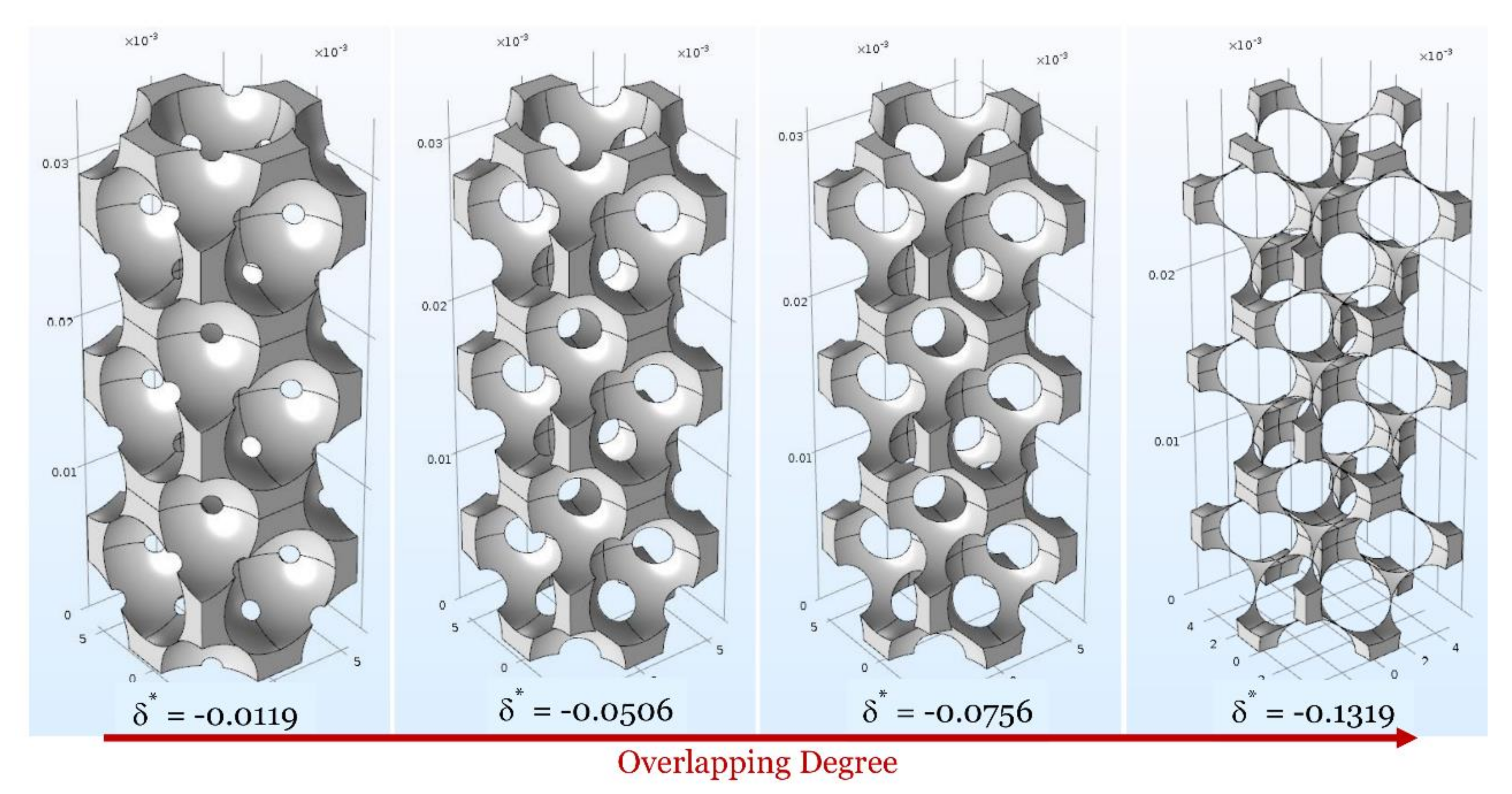
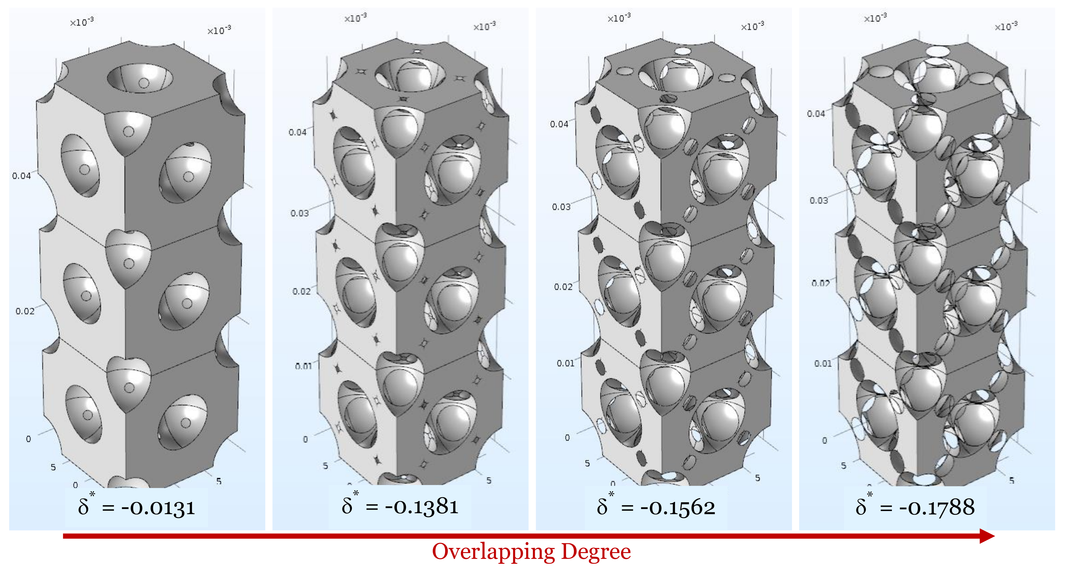
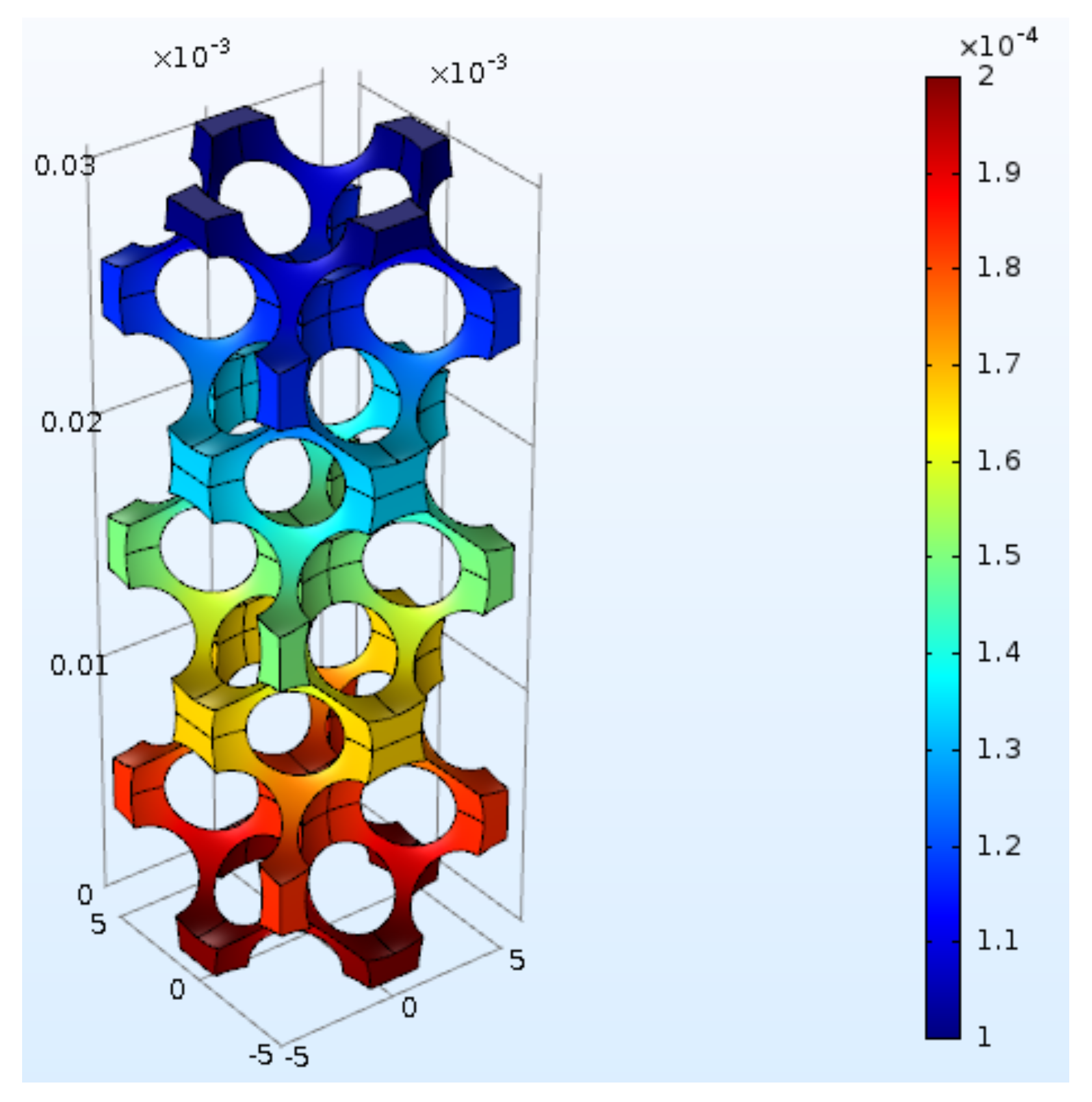
3.1. Stacks of Unit Cells
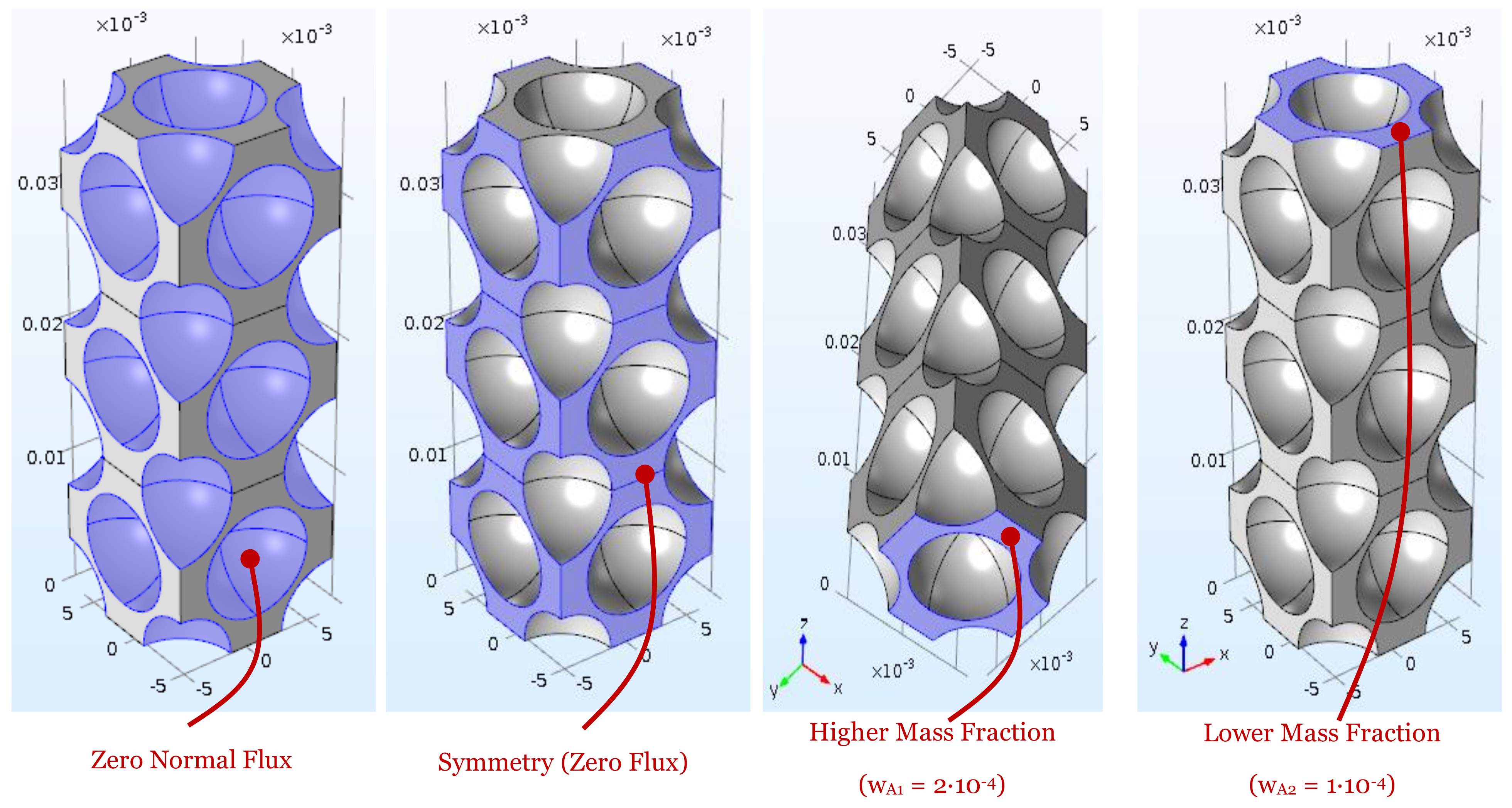
3.2. Computational Fluid Dynamic Approach
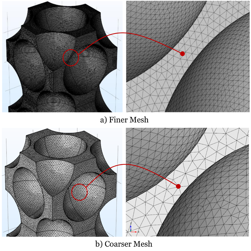
3.3. Mesh Setup
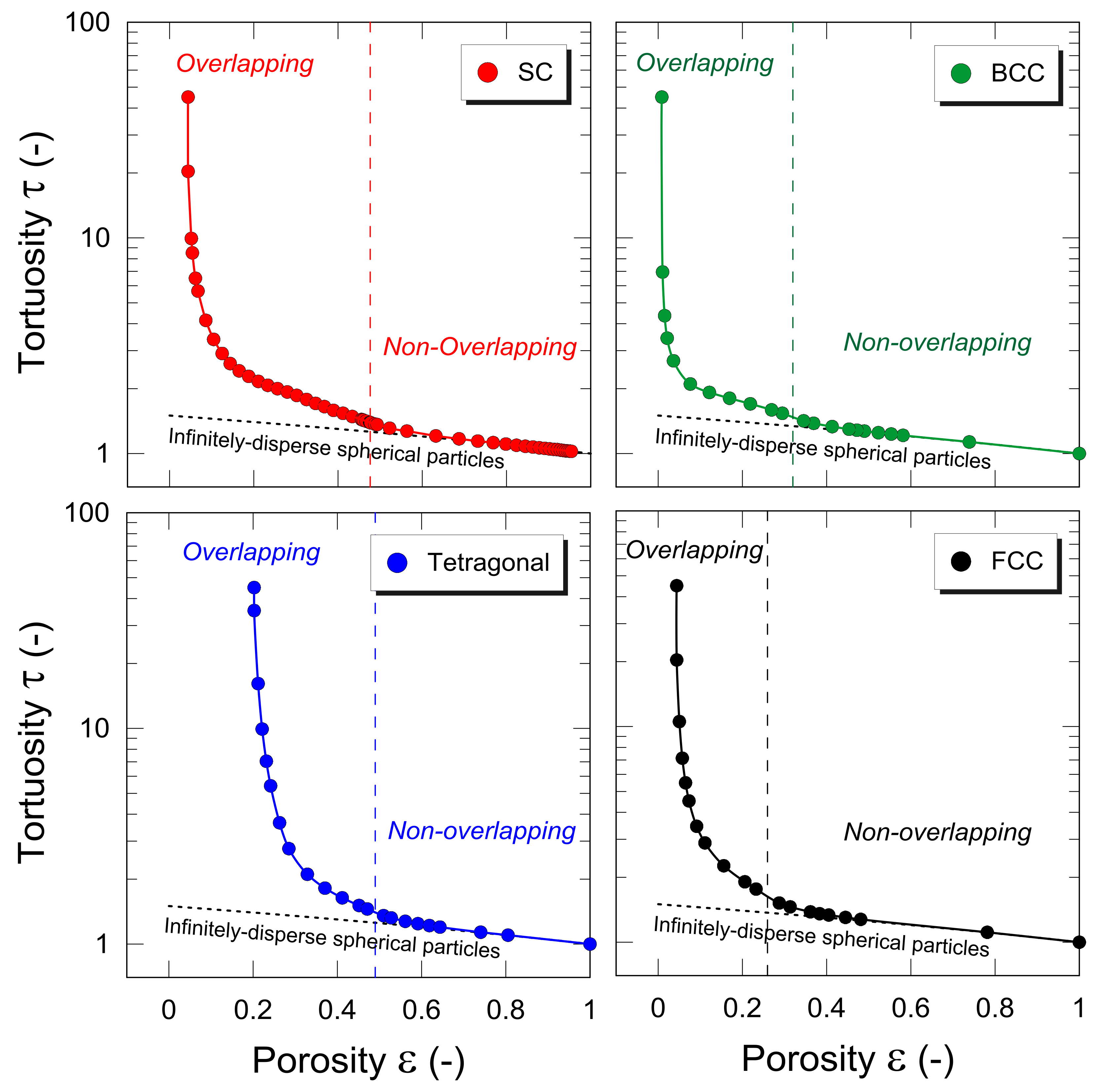
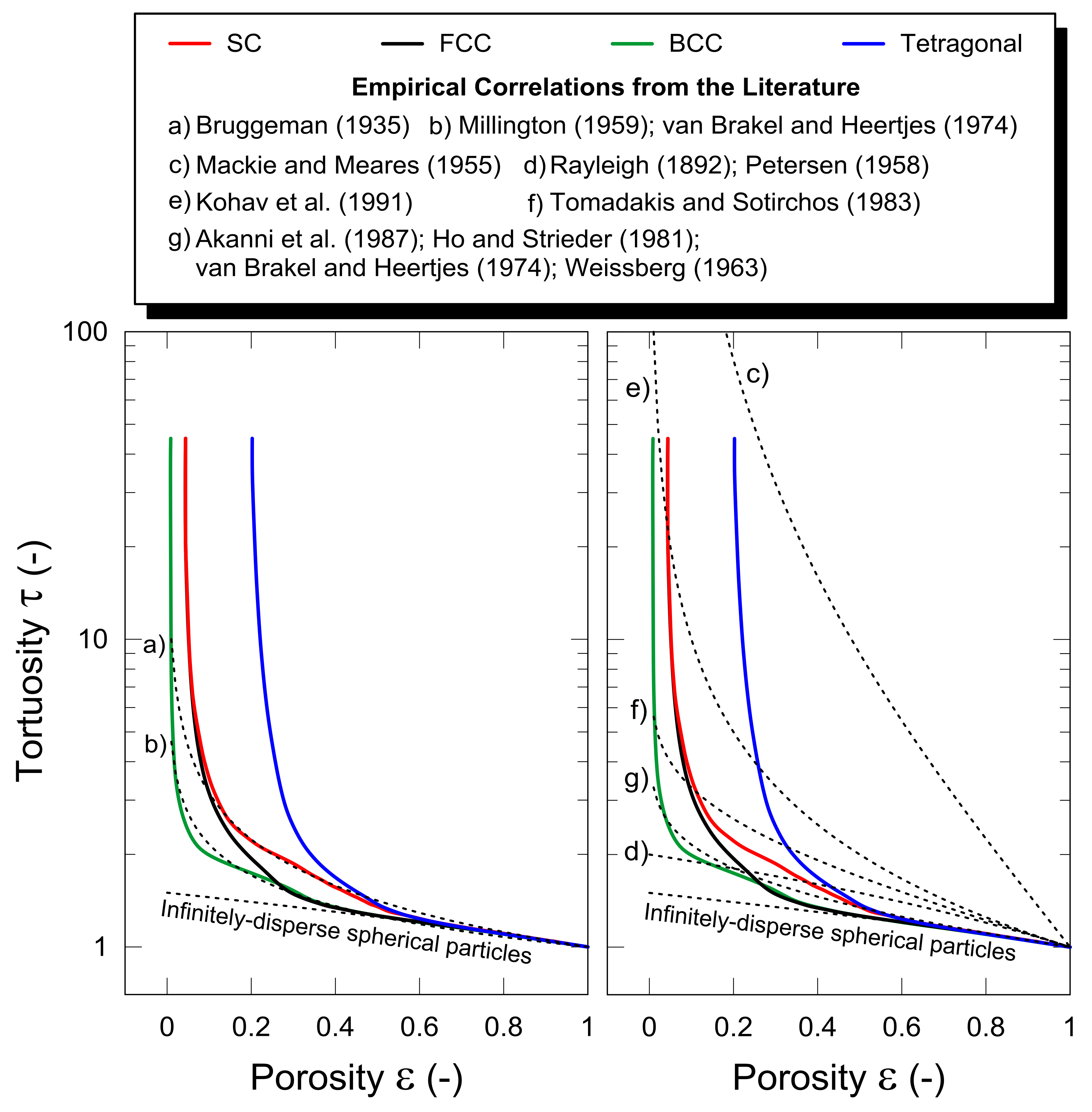
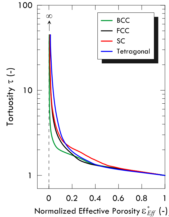
4. Results and Discussion
5. Conclusions
Acknowledgments
Author Contributions
Conflicts of Interest
References
- Chiappetta, G.; Clarizia, G.; Drioli, E. Theoretical analysis of the effect of catalyst mass distribution and operation parameters on the performance of a Pd-based membrane reactor for water-gas shift reaction. Chem. Eng. J. 2008, 136, 373–382. [Google Scholar] [CrossRef]
- Li, A.; Lim, C.J.; Grace, J.R. Staged-separation membrane reactor for steam methane reforming. Chem. Eng. J. 2008, 138, 452–459. [Google Scholar] [CrossRef]
- Caravella, A.; Di Maio, F.P.; Di Renzo, A. Computational Study of Staged Membrane Reactor Configurations for Methane Steam Reforming: I. Optimization of Stage Lengths. AIChE J. 2010, 56, 248–258. [Google Scholar] [CrossRef]
- Caravella, A.; Di Maio, F.P.; Di Renzo, A. Computational Study of Staged Membrane Reactor Configurations for Methane Steam Reforming: II. Effect of Number of Stages and Catalyst Amount. AIChE J. 2010, 56, 259–267. [Google Scholar] [CrossRef]
- Caravella, A.; Di Maio, F.P.; Di Renzo, A. Optimization of membrane area and catalyst distribution in a permeative-stage membrane reactor for methane steam reforming. J. Membr. Sci. 2008, 321, 209–221. [Google Scholar] [CrossRef]
- Lichtner, A.Z.; Jauffrès, D.; Roussel, D.; Charlot, F.; Martin, C.L.; Bordia, R.K. Dispersion, connectivity and tortuosity of hierarchical porosity composite SOFC cathodes prepared by freeze-casting. J. Eur. Ceram. Soc. 2015, 35, 585–595. [Google Scholar] [CrossRef]
- Promentilla, M.A.B.; Sugiyama, T.; Hitomi, T.; Takeda, N. Quantification of tortuosity in hardened cement pastes using synchrotron- based X-ray computed microtomography. Cement Concrete Res. 2009, 39, 548–557. [Google Scholar] [CrossRef]
- Guo, P. Dependency of Tortuosity and Permeability of Porous Media on Directional Distribution of Pore Voids. Transp. Porous Media 2012, 95, 285–303. [Google Scholar] [CrossRef]
- Kong, W.; Zhang, Q.; Gao, X.; Zhang, J.; Chen, D.; Su, S. A Method for Predicting the Tortuosity of Pore Phase in Solid Oxide Fuel Cells Electrode. Int. J. Electrochem. Sci. 2015, 10, 5800–5811. [Google Scholar]
- Popova, L.; van Dusschoten, D.; Nagel, K.A.; Fiorani, F.; Mazzola, B. Plant root tortuosity: An indicator of root path formation in soil with different composition and density. Ann. Bot. 2016, 118, 685–698. [Google Scholar] [CrossRef] [PubMed]
- Manickam, S.S.; Gelb, J.; McCutcheon, J.R. Characterization of Thin Film Composite Membranes Using Porosimetry and X-ray Microscopy. Microsc. Microanal. 2013, 19, 634–635. [Google Scholar] [CrossRef]
- Wiedenmann, D.; Keller, L.; Holzer, L.; Stojadinovic, J.; Munch, B.; Suarez, L.; Fumey, B.; Hagendorfer, H.; Bronnimann, R.; Modregger, P.; et al. Three-Dimensional Pore Structure and Ion Conductivity of Porous Ceramic Diaphragms. AIChE J. 2013, 59, 1446–1457. [Google Scholar] [CrossRef]
- Landesfeind, J.; Hattendorff, J.; Ehrl, A.; Wall, W.A.; Gasteiger, H.A. Tortuosity Determination of Battery Electrodes and Separators by Impedance Spectroscopy. J. Electrochem. Soc. 2016, 163, A1373–A1387. [Google Scholar] [CrossRef]
- Epstein, N. On Tortuosity and the Tortuosity Factor in Flow and Diffusion through Porous Media. Chem. Eng. Sci. 1989, 44, 777–779. [Google Scholar] [CrossRef]
- Ghanbarian, B.; Hunt, A.G.; Ewing, R.P.; Sahimi, M. Tortuosity in porous media—A critical review. Soil Sci. Soc. Am. J. 2013, 77, 1461–1477. [Google Scholar] [CrossRef]
- Carman, P.C. Fluid flow through a granular bed. Trans. Inst. Chem. Eng. 1937, 15, 150–167. [Google Scholar] [CrossRef]
- Carman, P.C. Flow of Gases through Porous Media; Academic Press: New York, NY, USA, 1956. [Google Scholar]
- Scheidegger, A.E. The Physics of Flow through Porous Media; University of Toronto Press: Toronto, ON, Canada, 1974. [Google Scholar]
- Kim, J.H.; Ochoa, J.A.; Whitaker, S. Diffusion in anisotropic media. Transp. Porous Media 1987, 2, 327–356. [Google Scholar] [CrossRef]
- Whitaker, S. Simultaneous heat, mass and momentum transfer in porous media: A theory of drying. Adv. Heat Transf. 1977, 13, 119–203. [Google Scholar]
- Quintard, M. Diffusion in isotropic and anisotropic porous systems: Three- dimensional calculations. Transp. Porous Media 1993, 11, 187–199. [Google Scholar] [CrossRef]
- Quintard, M.; Whitaker, S. Transport in ordered and disordered porous media: Volume-averaged equations, closure problems and comparison with experiments. Chem. Eng. Sci. 1993, 48, 2537–2564. [Google Scholar] [CrossRef]
- Gao, H.Y.; He, Y.H.; Zou, J.; Xu, N.P.; Liu, C.T. Tortuosity factor for porous FeAl intermetallics fabricated by reactive synthesis. Trans. Nonferr. Met. Soc. China 2012, 22, 2179–2183. [Google Scholar] [CrossRef]
- Pisani, L. Simple Expression for the Tortuosity of Porous Media. Transp. Porous Media 2011, 88, 193–203. [Google Scholar] [CrossRef]
- Caravella, A.; Hara, S.; Obuchi, A.; Uchisawa, J. Role of the bi-dispersion of particle size on tortuosity in isotropic structures of spherical particles by three-dimensional computer simulation. Chem. Eng. Sci. 2012, 84, 351–371. [Google Scholar] [CrossRef]
- Maxwell, J.C. Treatise on Electricity and Magnetism, 2nd ed.; Clarendon Press: Oxford, UK, 1881; Volume I. [Google Scholar]
- Neale, G.H.; Nader, W.K. Prediction of transport processes within porous media, Diffusive flow processes within a homogeneous swarm of spherical particles. AlChE J. 1973, 19, 112–119. [Google Scholar] [CrossRef]
- Solorzano, E.; Pardo-Alonso, S.; Brabant, L.; Vicente, J.; Van Hoorebeke, L.; Rodríguez-Pérez, M.A. Computational Approaches for Tortuosity Determination in 3D Structures. In Proceedings of the 1st International Conference on Tomography of Materials and Structures (ICTMS 2013), Ghent, Belgium, 1–5 July 2013; pp. 71–74. Available online: https://biblio.ugent.be/publication/4178455/file/4178457.pdf (accessed on 17 February 2018).
- Wang, P. Lattice Boltzmann Simulation of Permeability and Tortuosity for Flow through Dense Porous Media. Math. Prob. Eng. 2014. [Google Scholar] [CrossRef]
- Anovitz, L.M.; Cole, D.R. Characterization and Analysis of Porosity and Pore Structures. Rev. Mineral. Geochem. 2015, 80, 61–164. [Google Scholar] [CrossRef]
- Berg, C.F. Permeability Description by Characteristic Length, Tortuosity, Constriction and Porosity. Transp. Porous Media 2015, 103, 381–400. [Google Scholar] [CrossRef]
- Annunziata, R.; Kheirkhah, A.; Aggarwal, S.; Hamrah, P.; Trucco, E. A Fully Automated Tortuosity Quantification System with Application to Corneal Nerve Fibres in Confocal Microscopy Images. Med. Image Anal. 2016, 32, 216–232. [Google Scholar] [CrossRef] [PubMed] [Green Version]
- Deepagoda, T.K.K.C.; Moldrup, P.; Yoshikawa, S.; Kawamoto, K.; Komatsu, T.; Rolston, D.E. The gas-diffusivity-based Buckingham tortuosity factor from pF 1 to 6.91 as a soil structure fingerprint. In Proceedings of the 19th World Congress of Soil Science, Soil Solutions for a Changing World, Brisbane, Australia, 1–6 August 2010; pp. 2008–2011. [Google Scholar]
- Vallavh, R. Modeling Tortuosity in Fibrous Porous Media using Computational Fluid Dynamics. Ph.D. Thesis, North Carolina State University, Raleigh, NC, USA, 2009. [Google Scholar]
- Chen-Wiegart, Y.C.K.; Demike, R.; Erdonmez, C.; Thornton, K.; Barnett, S.A.; Wang, J. Tortuosity characterization of 3D microstructure at nano-scale for energy storage and conversion materials. J. Power Sources 2014, 249, 349–356. [Google Scholar] [CrossRef]
- Moldrup, P.; Olesen, T.; Komatsu, T.; Schjonning, P.; Rolston, D.E. Tortuosity, Diffusivity, and Permeability in the Soil Liquid and Gaseous Phases. Soil Sci. Soc. Am. J. 2001, 65, 613–623. [Google Scholar] [CrossRef]
- Kim, A.S.; Chen, H. Diffusive tortuosity factor of solid and soft cake layers: A random walk simulation approach. J. Membr. Sci. 2006, 279, 129–139. [Google Scholar] [CrossRef]
- Rezanezhad, F.; Quinton, W.L.; Price, J.S.; Elrick, D.; Elliot, T.R.; Heck, R.J. Examining the effect of pore size distribution and shape on flow through unsaturated peat using 3-D computed tomography. Hydrol. Earth Syst. Sci. Discuss. 2009, 6, 3835–3862. [Google Scholar] [CrossRef]
- Matyka, M.; Khalili, A.; Koza, Z. Tortuosity-porosity relation in porous media flow. Phys. Rev. E 2008, 78, 026306. [Google Scholar] [CrossRef] [PubMed]
- Luquot, L.; Rodriguez, O.; Gouze, P. Experimental Characterization of Porosity Structure and Transport Property Changes in Limestone Undergoing Different Dissolution Regimes. Transp. Porous Media 2014, 101, 507–532. [Google Scholar] [CrossRef]
- Shen, L.; Chen, Z. Critical review of the impact of tortuosity on diffusion. Chem. Eng. Sci. 2007, 62, 3748–3755. [Google Scholar] [CrossRef]
- Melo, L.F. Biofilm physical structure, internal diffusivity and tortuosity. Water Sci. Technol. 2005, 52, 77–84. [Google Scholar]
- Promentilla, M.A.B.; Sugiyama, T. Studies on 3D Micro-Geometry and Diffusion Tortuosity of Cement-Based Materials Using X-ray Microtomography. In Proceedings of the 32nd Conference on Our World in Concrete & Structures, Singapore, 28–29 August 2007. [Google Scholar]
- Mackie, J.S.; Meares, P. The diffusion of electrolytes in a cation exchange resin membrane. Proc. R. Soc. A 1955, 232, 498–509. [Google Scholar] [CrossRef]
- Elias-Kohav, T.; Moshe, S.; Avnir, D. Steady-state diffusion and reactions in catalytic fractal porous media. Chem. Eng. Sci. 1991, 46, 2787–2798. [Google Scholar] [CrossRef]
- Rayleigh, L. On the influence of obstacles arranged in rectangular order upon the properties of a medium. Philos. Mag. 1892, 34, 481–489. [Google Scholar] [CrossRef]
- Bruggeman, D.A. Berechnung verschiedener physikalischer Konstanten von heterogenen Substanzen. I. Dielektrizitätskonstanten und Leitfähigkeiten der Mischkörper aus isotropen Substanzen. Ann. Phys. 1935, 24, 636–664. [Google Scholar] [CrossRef]
- Petersen, E.E. Diffusion in a pore of varying cross section. AIChE J. 1958, 4, 343–345. [Google Scholar] [CrossRef]
- Millington, R.J. Gas diffusion in porous media. Science 1959, 130, 100–102. [Google Scholar] [CrossRef] [PubMed]
- Tomadakis, M.M.; Sotirchos, S.V. Transport properties of random arrays of freely overlapping cylinders with various orientation distributions. J. Chem. Phys. 1983, 98, 616–626. [Google Scholar] [CrossRef]
- van Brakel, J.; Heertjes, P.M. Analysis of diffusion in macroporous media in terms of a porosity, a tortuosity and a constrictivity factor. Int. J. Heat Mass Transf. 1974, 17, 1093–1103. [Google Scholar] [CrossRef]
- Weissberg, H. Effective diffusion coefficients in porous media. J. Appl. Phys. 1963, 34, 2636–2639. [Google Scholar] [CrossRef]
- Akanni, K.A.; Evans, J.W.; Abramson, I.S. Effective transport coefficients in heterogeneous media. Chem. Eng. Sci. 1987, 42, 1945–1954. [Google Scholar] [CrossRef]
- Ho, F.G.; Strieder, W. A variational calculation of the effective surface diffusion coefficient and tortuosity. Chem. Eng. Sci. 1981, 36, 253–258. [Google Scholar] [CrossRef]


| Mesh | τ (-) |
|---|---|
| Finer | 1.35535 |
| Coarser | 1.35674 |
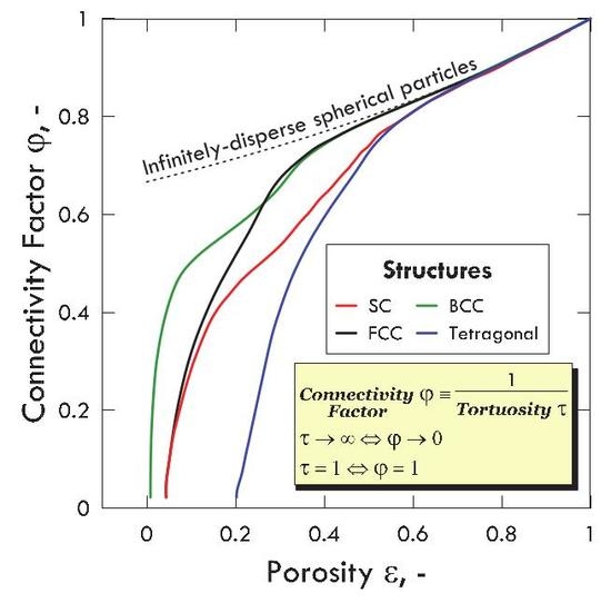
| Structure | εLim |
|---|---|
| SC | 0.035498 |
| BCC | 0.005956 |
| FCC | 0.036110 |
| Tetragonal | 0.191913 |
| Expression | Range of Application | References |
|---|---|---|
| Porous structures with a hyperbola of revolution as a pore model | Rayleigh (1892) [46] Petersen (1958) [48] | |
| Composite heterogeneous porous media | Bruggeman (1935) [47] | |
| Partially saturated homogeneous isotropic monodisperse sphere packing | Millington (1959) [49] van Brakel and Heertjes (1974) [51] | |
| Overlapping spheres | Akanni et al. (1987) [53] Ho and Strieder (1981) [54] van Brakel and Heertjes (1974) [51] Weissberg (1963) [52] | |
| Random arrays of freely overlapping cylinders | Tomadakis and Sotirchos (1983) [50] | |
| Catalytic fractal porous media | Kohav et al. (1991) [45] | |
| Cation-exchange resin membrane | Mackie and Meares (1955) [44] |
© 2018 by the authors. Licensee MDPI, Basel, Switzerland. This article is an open access article distributed under the terms and conditions of the Creative Commons Attribution (CC BY) license (http://creativecommons.org/licenses/by/4.0/).
Share and Cite
Bellini, S.; Azzato, G.; Grandinetti, M.; Stellato, V.; De Marco, G.; Sun, Y.; Caravella, A. A Novel Connectivity Factor for Morphological Characterization of Membranes and Porous Media: A Simulation Study on Structures of Mono-Sized Spherical Particles. Appl. Sci. 2018, 8, 573. https://doi.org/10.3390/app8040573
Bellini S, Azzato G, Grandinetti M, Stellato V, De Marco G, Sun Y, Caravella A. A Novel Connectivity Factor for Morphological Characterization of Membranes and Porous Media: A Simulation Study on Structures of Mono-Sized Spherical Particles. Applied Sciences. 2018; 8(4):573. https://doi.org/10.3390/app8040573
Chicago/Turabian StyleBellini, Stefano, Giulia Azzato, Monia Grandinetti, Virgilio Stellato, Giuseppe De Marco, Yu Sun, and Alessio Caravella. 2018. "A Novel Connectivity Factor for Morphological Characterization of Membranes and Porous Media: A Simulation Study on Structures of Mono-Sized Spherical Particles" Applied Sciences 8, no. 4: 573. https://doi.org/10.3390/app8040573