Path Planning Method for Manipulators Based on Improved Twin Delayed Deep Deterministic Policy Gradient and RRT*

Abstract

This paper proposes a path planning framework that combines the experience replay mechanism from deep reinforcement learning (DRL) and rapidly exploring random tree star (RRT*), employing the DRL-RRT* as the path planning method for the manipulator. The iteration of the RRT* is conducted independently in path planning, resulting in a tortuous path and making it challenging to find an optimal path. The setting of reward functions in policy learning based on DRL is very complex and has poor universality, making it difficult to complete the task in complex path planning. Aiming at the insufficient exploration of the current deterministic policy gradient DRL algorithm twin delayed deep deterministic policy gradient (TD3), a stochastic policy was combined with TD3, and the performance was verified on the simulation platform. Furthermore, the improved TD3 was integrated with RRT* for performance analysis in two-dimensional (2D) and three-dimensional (3D) path planning environments. Finally, a six-degree-of-freedom manipulator was used to conduct simulation and experimental research on the manipulator.

1. Introduction

The utilization of multi-degree-of-freedom manipulators is prevalent across various industries including aerospace and industrial manufacturing and so on. The study of path planning problem in complex environments is a crucial aspect in the field of robot control technology. At present, some path planning methods commonly employed include the A* algorithm based on graph traversals [1], the probabilistic roadmap method (PRM) algorithm based on probability sampling [2] and rapidly exploring random tree star (RRT*) utilizing a random sampling technique [3,4]. Informed RRT* uses a heuristic function to guide exploration toward the target region by optimizing the sampling process [5]. RRT*-Smart enhances the optimization speed of paths near obstacle turning points by incorporating path optimization and intelligent sampling techniques within RRT* [6]. The node generation strategy of the Gaussian mixture model RRT* (GMM-RRT*) algorithm utilizes a target-biased policy, resulting in shorter path length [7]. The P-RRT*-connect [8] combines the bidirectional artificial potential field with RRT*, which reduces the time and decreases the number of iterations. The Real-Time RRT* (RT-RRT*) [9] introduces an online tree rewiring strategy, it can find paths to new targets more quickly. These methods exhibit robust environmental exploration abilities, asymptotic optimality and consume fewer computational resources. However, these methods explore the environment randomly and hardly use valuable previous iterative experience to guide sampling. This characteristic may lead to these methods unable to find more optimized solutions.

The introduction of Deep Q-network (DQN) by [10] marked a milestone in the field. DRL has achieved remarkable advancements in many fields [11,12,13]. DRL empowers agents to conduct autonomous exploration and leverage the experience gained from prior explorations to inform subsequent behavioral decisions. With the advent of DRL, robots are now capable of self-directed learning. The Refs. [14,15] proposed a path planning method of improved learning policy based on different experience depth requirements at different learning stages. Marcin et al used deep deterministic policy gradient (DDPG) [16] and hindsight experience replay (HER) to train the manipulator in a simulated environment [17]. Gu [18] used a policy learning algorithm with deep Q-function to train physical robots. Lin [19] used recurrent neural network and DDPG to predict the collision-free path. Yang [20] proposed a new deep Q-learning method, which was applied to the push and grasp of objects by manipulators. Li [21] proposed a DRL that integrates automatic entropy adjustment. Kim [22] designed a motion planning algorithm that uses TD3 [23] with HER to enhance sample efficiency.

Some advanced DRL algorithms possess certain limitations. Pan [24] used the Boltzmann Softmax operator to estimate the value function, which increased computational costs and involved an amount of parameter adjustment. The policy of DRL is driven by reward during learning, successful learning relies on the design of reward functions and an action selection policy to ensure exploration and exploitation [25]. The universality of the reward function is typically low, and its design poses significant challenges. In the presence of obstacles, employing a general distance-based reward function often leads to policy learning failures [26]. Li [27] layered the DRL model to avoid the construction of complex reward functions. The task or policy model is divided into upper and lower layers to mitigate the coupling between the update formula and the challenging convergence of the reward function [28].

The challenge of applying DRL to path planning tasks remains significant. The current trend is to combine DRL with traditional path planning methods. The traditional path planning methods, such as RRT and PRM, possess robust sampling and search abilities, enabling them to provide reference paths or intermediate waypoints for DRL. In turn, DRL accomplishes the point-to-point task between each pair of nodes so that agents can obtain a smoother path [29]. Sampling path planning methods does not need a reward function in complex environment and has a higher success rate than does the DRL, it can be used to provide a successful experience reference for DRL, and DRL can use these experiences to exert exploration ability and finally complete the learning of the path planning strategy. Gao [30] combined TD3 with PRM, this can decompose the path into multiple local paths, improve development efficiency. Li [21] proposed traditional path planners with DRL to obtain the path in Cartesian space. Florensa [31] decomposed complex problems into multiple subproblems and explored maze paths using dynamic programming. Chiang et al. [32] regarded PRM and RRT as global path planning methods, respectively, and searched for intermediate path points of DRL in indoor navigation. The waypoint selection of some fusion methods is influenced by traditional path planning. To address the above issues, the contributions are outlined as follows:

• In order to improve the ability of DRL algorithm to balance exploration and development, an improved TD3 algorithm was designed and evaluated.
• Aiming at the problems existing in robot path planning, a path planning method is proposed that combines the exploration abilities of sampling-based RRT* and the experience replay mechanism of DRL algorithm.
• The simulation environment of path optimization based on DRL-RRT* is built.

The remaining sections of this paper are organized as follows: Section 2 presents the implementation principle of the proposed CDTD3 algorithm. Section 3 provides a detailed description of the DRL-RRT* path planning algorithm. Section 4 reports the path planning verification in a simulation environment. Section 5 outlines the experimental verification of the manipulator path planning using CDTD3-RRT*. Section 6 concludes the paper.

2. Improved TD3 Algorithm

2.1. Reinforcement Learning

Reinforcement learning (RL) are generally described using the Markov decision process (MDP) [33], and a tuple $M=(S,\mathcal{A},r,p,\gamma )$ can be used to describe MDP, where $S$ and $\mathcal{A}$ represent a set of states and actions, $p$ is the probability of transition from the current state to the next state, $r$ is the reward given by environmental changes for state transition, and $\gamma \in (0,1)$ is a discount used to determine reward priority. At time step $t$, for a given state $s\in S$, the agent can obtain $r$ by selecting action $a\in \mathcal{A}$ based on policy $\mu$ and transfer to the next state $s_{i+1}\in S$. The goal of the agent is to maximize the discounted return $R_t={\displaystyle {\sum }_{i=t}^T{\gamma }^{i-t}r(s_i,a_i)}$ [23], which can be measured by value function $Q$ shown in Equation (1).

$$Q^{\mu }(s,a)={\mathrm{E}}_{\mu }[R_t|s,a]$$

(1)

2.2. Algorithm Structure

The actor-critic structure DRL algorithm TD3 [23] for continuous control is advanced. Similar to popular DRL such as soft actor critical (SAC) [34], TD3 uses the double network structure of actor and critic. Both the current actor network ${\mu }_{\theta }(s)$ and the current critic network $Q_{{\omega }_k}(s,a)$ (k = 1, 2) have a corresponding target network, during the implementation, only ${\mu }_{\theta }(s)$ and $Q_{{\omega }_k}(s,a)$ participate in parameter update while the target actor network ${\mu }_{{\theta }^{\prime }}(s)$ and the target critic network $Q_{{{\omega }^{\prime }}_k}(s_{i+1},a^{\prime })$ (k = 1, 2) are used to store the parameters of the corresponding target network at the previous time. ${\mu }_{{\theta }^{\prime }}(s)$ and $Q_{{{\omega }^{\prime }}_k}(s_{i+1},a^{\prime })$ do not completely copy the parameters of their corresponding original network when storing them; instead, a soft update method shown in Equation (2) is adopted.

$$\left\{\begin{array}{l}{\theta }^{\prime }=\tau \theta +(1-\tau ){\theta }^{\prime }\\ {{\omega }^{\prime }}_k=\tau {\omega }_k+(1-\tau ){{\omega }^{\prime }}_k\end{array}\right.$$

(2)

where $\tau \in (0,1)$. $\theta$ and ${\theta }^{\prime }$ represent the network parameters of ${\mu }_{\theta }(s)$ and ${\mu }_{{\theta }^{\prime }}(s)$, respectively. ${\omega }_k$ and ${{\omega }^{\prime }}_k$ correspond to $Q_{{\omega }_k}(s,a)$ and $Q_{{{\omega }^{\prime }}_k}(s_{i+1},a^{\prime })$, respectively.

TD3 select an action based on policy ${\mu }_{\theta }(s_i)$ in the $s_i$. Due to the deterministic policy adopted by TD3, a certain proportion of random noise is added in the exploration phase to improve the exploration ability of the agent. The output of $a_i$ is shown in Equation (3).

$$a_i={\mu }_{\theta }(s_i)+\delta$$

(3)

where $\delta \sim \mathcal{N}(0,\sigma )$ represents a Gaussian distribution with a mean of 0 and variance $\sigma$. To limit the action, $a$ is cropped as $a_{low}<a<a_{high}$. The concept of off-policy DRL is to fully utilize previous experience memory, these algorithms usually have a large experience replay buffer $\mathcal{B}$, which is used to store information such as state, action, reward, and next state for each step. When updating the actor network and critic network, the required parameter sequence $\mathrm{\Gamma }=(s_i,a_i,r_i,s_{i+1})$ in the update equation will be obtained by sampling from the $\mathcal{B}$, and the objective function can be calculated using Equations (4) and (5).

$$y_i=r_i+\gamma \underset{k=1,2}{\min }{Q}_{{{\omega }^{\prime }}_k}(s_{i+1},a^{\prime })$$

(4)

$$a^{\prime }={\mu }_{{\theta }^{\prime }}(s_{i+1})+\xi$$

(5)

where $r_i$ is the reward, and $a^{\prime }$ represents the output of the network ${\mu }_{{\theta }^{\prime }}(s_{i+1})$ with noise $\xi$ and $\xi \sim \mathcal{N}(0,\tilde{\sigma })$ denoting a Gaussian distribution, which is clipped to $(-c,c)$ $c>0$. Adding clipped noise to the actions by ${\mu }_{{\theta }^{\prime }}(s_{i+1})$ is a regularization method that can be used to alleviate overfitting in the output of $Q_{{{\omega }^{\prime }}_k}(s_{i+1},a^{\prime })$. In Equation (4), the values of two target networks $Q_{{{\omega }^{\prime }}_k}(s_{i+1},a^{\prime })$ is minimized to reduce bias; otherwise, the update of the current critic network can be performed with Equation (6) to minimize the loss ${\mathcal{L}}_{\omega }$.

$${\mathcal{L}}_{\omega }=\frac{1}{N}{{\displaystyle \sum _{i=0}^N[y_i-Q_{{\omega }_k}(s_i,a_i)]}}^2$$

(6)

where $N$ is the number of batches sampled from $\mathcal{B}$. In deterministic policy gradient RL [35], the policy parameters are updated by calculating the sampled policy gradient. Equation (7) can be used to update the current actor network.

$${\mathcal{L}}_{\theta }=\frac{1}{N}{\displaystyle \sum _{i=0}^N[{\nabla }_a{Q}_{{\omega }_1}(s_i,a){|}_{a={\mu }_{\theta }(s_i)}{\nabla }_{\theta }{\mu }_{\theta }(s_i)]}$$

(7)

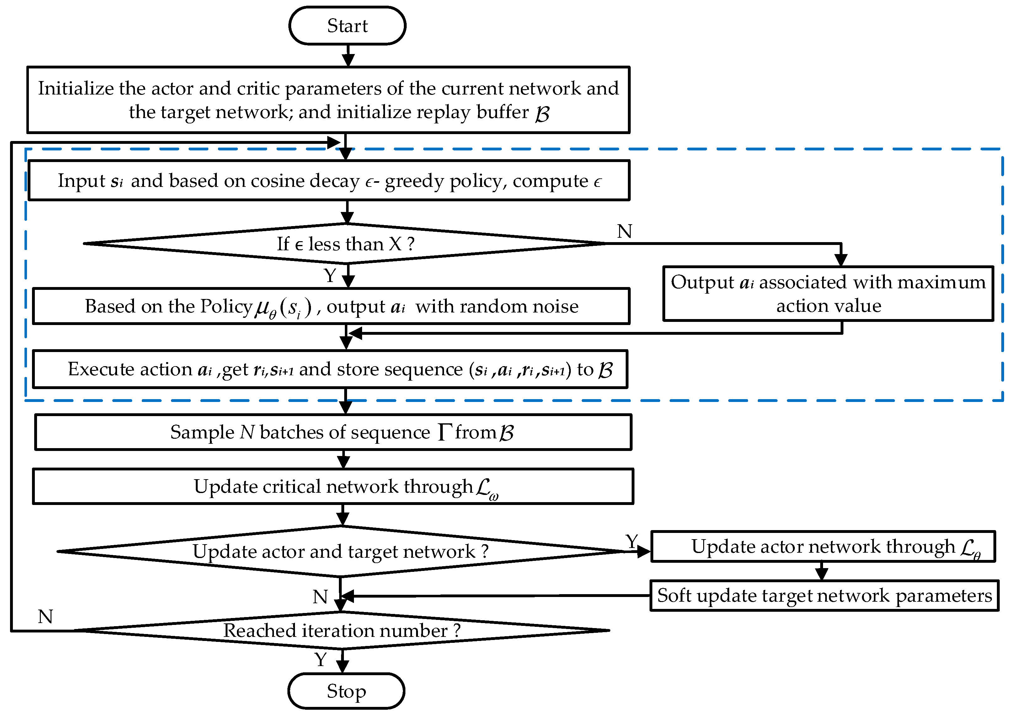
As shown in Equation (3), although adding a certain proportion of noise in the exploration stage of TD3 can increase a certain exploration ability, the deterministic policy plays a dominant role in the policy learning exploration, which still limits the early exploration of the agent. In order to enhance the exploration ability of the agent, ϵ-greedy is a commonly used policy for balancing exploitation and exploration. The ϵ-greedy policy is shown in Equation (8), which shows that when the agent makes a decision, there is a small probability of positive ϵ will randomly selecting an unknown action, and a probability of (1 − ϵ) will selecting the action with the largest action value among the existing actions.

$${\mu }_{\theta }(s_i)=\left\{\begin{array}{l}\frac{ϵ}{\left|A\right|}+1-ϵ , if a=\arg \max Q(s_i,a_i)\\ \frac{ϵ}{\left|A\right|} , \hspace{1em}\hspace{1em}\hspace{1em}if a\ne \arg \max Q(s_i,a_i)\end{array}\right.$$

(8)

A standard RL algorithm must include exploration and exploitation. Exploration helps the agent fully understand state space and select the other unknown action, and exploitation helps the agent find the optimal action to maximize the expected return at the present moment. Inspired by these methods, TD3 is combined with ϵ-greedy policy. In order to enhance the exploration ability of agent in the early stage and make more stable use of the exploration in the later stage, the decay of ϵ-greedy policy is used and combined with TD3. The ϵ-greedy policy proposed based on cosine decay as shown in Equation (9).

$$ϵ=\lambda (c+\cos (\frac{\pi t}{i}))$$

(9)

where $\lambda \in (0,0.5)$, c is a constant greater than 1, $i$ is training steps, and $t$ is the current step value. After combining TD3 with the ϵ-greedy policy of cosine decay, the method of action selection shown in Equation (3) can be changed to the form shown in Equation (10).

$$a_i=\left\{\begin{array}{cc}{\mu }_{\theta }(s_i)+\delta ,& if ϵ\le \mathrm{X}\\ \tilde{\delta },& if ϵ>\mathrm{X}\end{array}\right.$$

(10)

where $\mathrm{X}$ is the uniform distribution on [0,1); and $\tilde{\delta }\sim (0,{\sigma }^{\prime })$ is a random number conforming to a Gaussian distribution with a mean of 0 and a standard deviation of ${\sigma }^{\prime }$; it is common to set ${\sigma }^{\prime }$ to a number associated with the maximum action. The flow of the cosine decay TD3 (CDTD3) algorithm is shown in Figure 1.

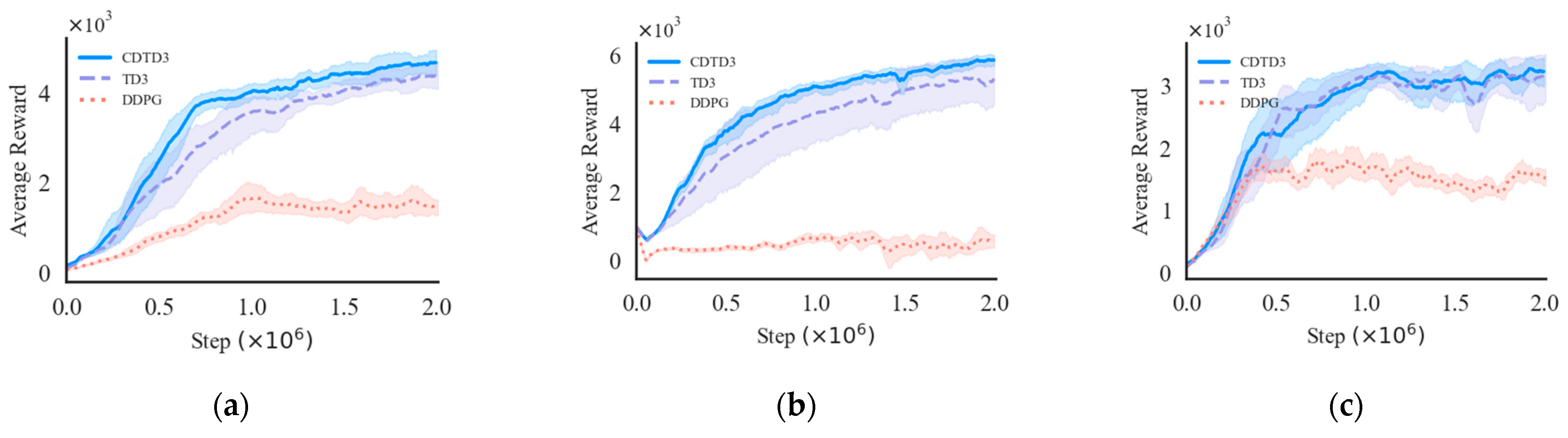
The performance of CDTD3 was tested in MuJoCo through the OpenAI Gym interface. The original task set was used during testing without modifying the environment and reward function. Except for the individual characteristics of the algorithms, other settings remained the same. Each algorithm was run 10 times under different random seeds. The number of training steps in each task was two million steps. The results are shown in Figure 2, including the results of three different DRL algorithms running on three different robot tasks in MuJoCo. The dimensions of the robot’s joints in Figure 2a–c from more to less, and the specified task difficulty ranges from hard to easy. The x-axis is the number of steps, while the y-axis is the average return of ten evaluations per five thousand steps for the current task under two million training steps. The shaded area in the Figure 2 represents the maximum and minimum value intervals with test data smoothed by convolution, while the solid line represents the average of ten experimental results.

In Figure 2c, the robust exploratory ability of CDTD3 does not significantly contribute to relatively simple tasks. However, in the scenarios illustrated in Figure 2a,b, CDTD3 exhibits a superior ability to explore actions with higher rewards and to rapidly incorporate them into decision-making process compared to the TD3. CDTD3 has strong exploration ability and adaptability to tasks, which makes policy learning more efficient.

3. The Improved Path Planning Method

RRT* has the characteristics of continuous iteration and path replanning in the environment. However, due to its random nature, each exploration or iteration of RRT* is independent of each other, so the new node positions generated by each iteration may be different, leading to a tortuous and suboptimal path. The reward function in DRL plays a pivotal role in shaping the learning effectiveness of the agent. It is imperative to define an appropriate reward function for each task to guide the agent toward successful task completion. The variation of the task can also easily lead to the failure of the reward function.

Currently, there are many improved variations of RRT*, such as informed RRT* [5], RRT*-Smart [6], and real-time RRT* [9], which have advantages in specific scenarios. However, they still face the problem of independent exploration and iteration. Additionally, introducing target biasing methods in RRT* can yield favorable results, and this approach is relatively easier to implement and debug compared to algorithms such as informed RRT*. Based on these issues, a path planning framework that combines the strengths of DRL and RRT* have been proposed, and is built on the basis of RRT* with target bias.

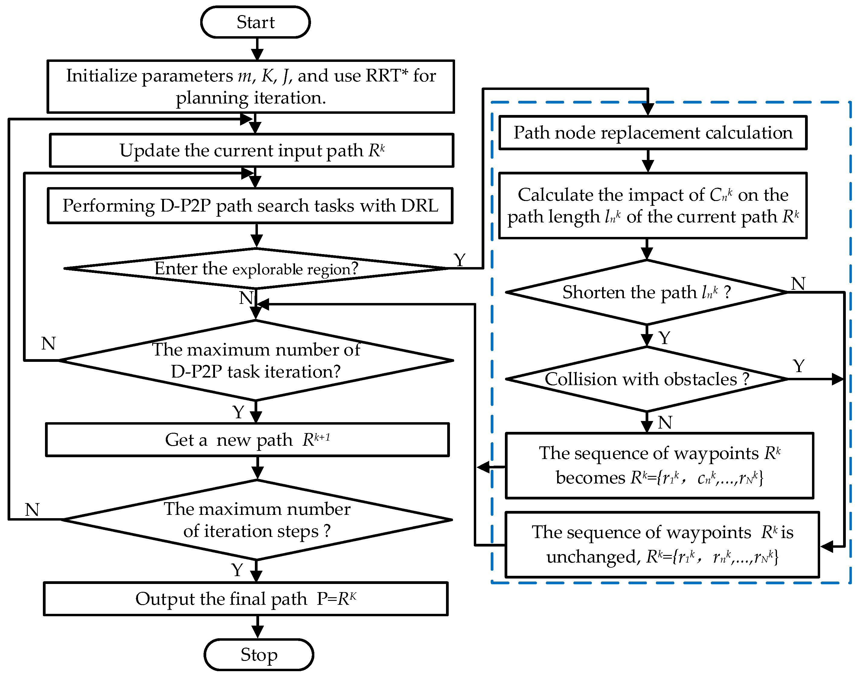
Performing a path search between two adjacent waypoints is called a dynamic point-to-point (D-P2P) task. The agent defines a spherical range centered at the intermediate waypoint as an explorable region and performs a D-P2P task between the preceding and following waypoint. The initial base path $R^0=\{{r_1}^0,{r_2}^0,\dots ,{r_N}^0\}$ is obtained by RRT*, $N$ is the total number of waypoints. The length of the original path can be characterized as $l_0^1={\displaystyle {\sum }_{n=1}^{N-1}\left|r_n^1{r}_{n+1}^1\right|}$, where $\left|r_n^1{r}_{n+1}^1\right|$ represents the Euclidean distance between waypoints $r_n^1$ and $r_{n+1}^1$.The steps of the DRL-RRT* algorithm is described as follows.

Step 1: Initialization. The number of iterations for RRT* is m, DRL path search task is K times. D-P2P task for each iteration is J = N − 2 groups. Using RRT* for planning iteration.

Step 2: Using DRL for path search tasks. When the agent first enters the $j$$th$ $(1\le j\le J)$ explorable region in a certain steps, the position $c_j^k$ is retained as the end position of this D-P2P task, and the waypoint replacement task in Step 3 is performed. If the explorable region is not accessed in the specified number of steps, go to Step 4.

Step 3: The procedure of waypoint replacement. The first waypoint replacement is considered, resulting in point $c_2^1$ being obtained after completion of the D-P2P task; then, the impacts of $r_2^1$ and $c_2^1$ on the original path are computed individually. If $c_2^1$ makes the path shorter, $c_2^1$ replaces $r_2^1$, and the length becomes $l_0^1=\left|r_1^1{c}_2^1\right|+\left|c_2^1{r}_3^1\right|+{\displaystyle {\sum }_{n=3}^{N-1}\left|r_n^1{r}_{n+1}^1\right|}$. The waypoints of the path become $R^1=\{{\mathrm{r}}_1^1,c_2^1,\dots ,r_N^1\}$; at the same time, $c_2^1$ also serves as the starting position for the next D-P2P task; otherwise, the original path is unchanged.

Step 4: Termination condition check for a round of DRL search task. If D-P2P task iteration is larger than the iterative number J, break to Step 2.

Step 5: Get the new path $R^{k+1}$. Assuming that only $c_2^1$ can shorten the path during the first iteration (k = 1), the path for the second iteration is $R^2=\{{\mathrm{r}}_1^2,{\mathrm{r}}_2^2,\dots ,r_N^2\}=\{{\mathrm{r}}_1^1,c_2^1,\dots ,r_N^1\}$.

Step 6: Terminating condition check. If the iteration is larger than K, the path explored is retained as $P=R^K$, and the algorithm stops. Otherwise, restart from Step 2.

RRT* with DRL is utilized by Kontoudis [29]; however, the waypoints were unchanged during the process. Reference [30] employed TD3 and PRM as a path planning method, in such cases, the final path is highly influenced by the original path, limiting the effectiveness of the DRL in path planning. In contrast, in the proposed DRL-RRT*, DRL optimizes the underlying path planned by RRT* by automatically adjusting the intermediate nodes of the path. Consequently, potential optimizations can be explored, allowing for direct modification of the underlying path. Reference [21] combined improved DRL with RRT*, and optimized the path by adjusting the intermediate waypoints. In contrast, the proposed method calculates the path replacement as soon as the intermediate waypoints are explored, and the path replacement method is simpler. Base on the planning results of RRT*, the policy learning and experience replay mechanism of DRL are combined to obtain a better path. Figure 3 illustrates the flow of the proposed DRL-RRT* path optimization algorithm.

In each iteration of length optimization, the agent using DRL performs a D-P2P path search task. In each task, the reward function is designed as follows:

$$r=\left\{\begin{array}{cc}\frac{\alpha }{e^{-\rho d}},& other\\ 0,& if collsion\end{array}\right.$$

(11)

where d is the distance between the agent and the goal. To ensure an appropriate reward value in D-P2P tasks, constants $\alpha$ and $\rho$ are introduced to limit its magnitude. It is crucial to keep $0<\rho <1$ to avoid potential issues such as vanishing or exploding gradients.

4. Simulation Analysis

When the DRL-RRT* is used for path optimization simulation in 2D and 3D obstacle environments, the success rate of each path iteration optimization is expressed as follows:

$$\eta =\frac{1}{K}\frac{1}{J}{\displaystyle \sum _{k=1}^K{\displaystyle \sum _{j=1}^J{\zeta }_j^k}}\times 100\%$$

(12)

where $K$ represents the number of path search tasks performed by DRL, J represents the number of groups for D-P2P tasks, and ${\zeta }_j^k\in \{0,1\}$. If the agent can reach the endpoint of the current task in the maximum step size of the $j$ D-P2P tasks in $k$ times iteration, then ${\zeta }_j^k=1$; otherwise, ${\zeta }_j^k=0$.

4.1. Analysis of the 2D Simulation Environment

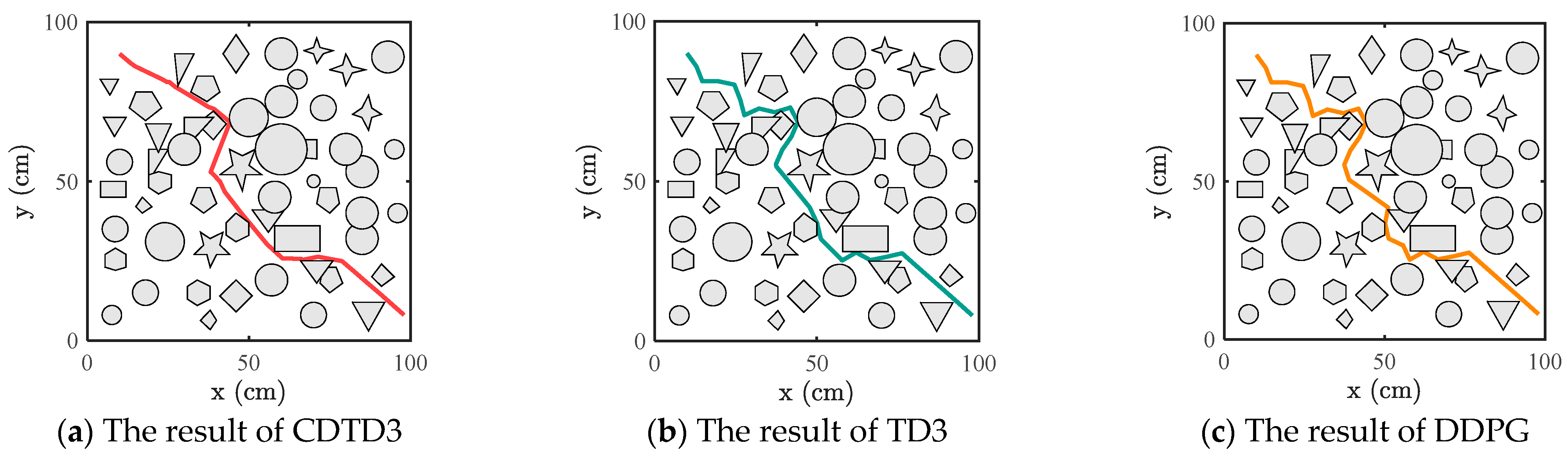
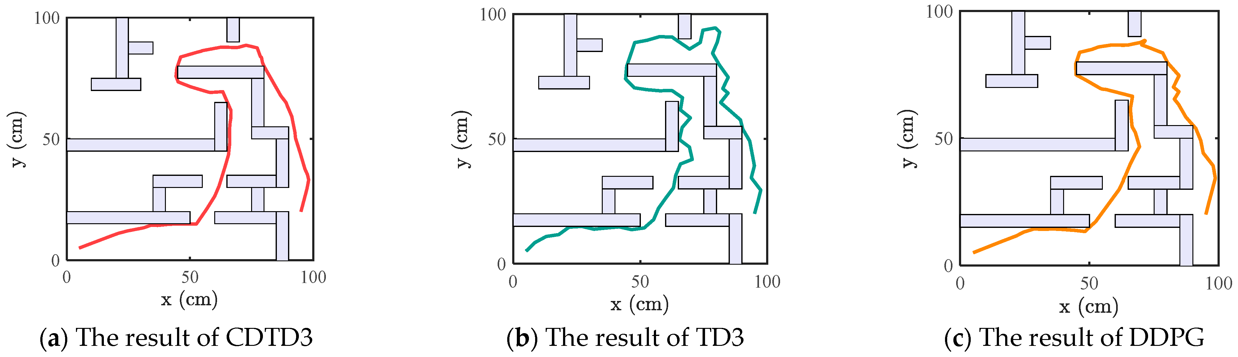
The size of the 2D complex obstacle environment was 100 (cm²), and the simulation environment was configured with obstacles of diverse shapes is depicted in Figure 4, the lines represent the paths and the gray geometric objects represent obstacles. The starting position was (10, 90), and the target position was (98, 8). In order to fully utilize the exploration ability of RRT*, a target bias strategy is introduced in RRT*, which makes the sampling point equal to the target point with a certain probability $p$ and randomly samples with a probability of $(1-p)$.

RRT* was first used for 10,000 iterations in the 2D simulation scenario. Then, CDTD3, TD3, and DDPG are used for 100 iterations of path optimization experiments on the DRL-RRT* algorithm, respectively. Iteration steps K in each experiment was 200, and the steps in each D-P2P task was 200. Among the 100 times experiments of each algorithm in each environment, different experiments were configured with different random seeds. The resulting path is shown in Figure 4, and the path optimized using the CDTD3 demonstrated improvements in terms of both path length and smoothness, closely resembling a straight line throughout most of the obstacle-free sections.

As DDPG and TD3 use a deterministic policy, they are prone to premature convergence to local optima with fixed actions during the continuous exploration and optimization process, making it difficult to explore better policy. They performed worse than did CDTD3 in terms of path length and success rate. The addition of a random exploration mechanism in CDTD3 enhances the exploration ability of the deterministic policy DRL and prevents premature convergence to local optima which includes fixed action selection. This feature can help the agent to be more inclined to explore the environment in the early stage of the task so as to explore a better policy. In certain obstacle-free spaces, CDTD3 explored and identified more optimal waypoints. By replacing intermediate waypoints through point substitution, the originally curved paths become straighter and the length of the path is shortened.

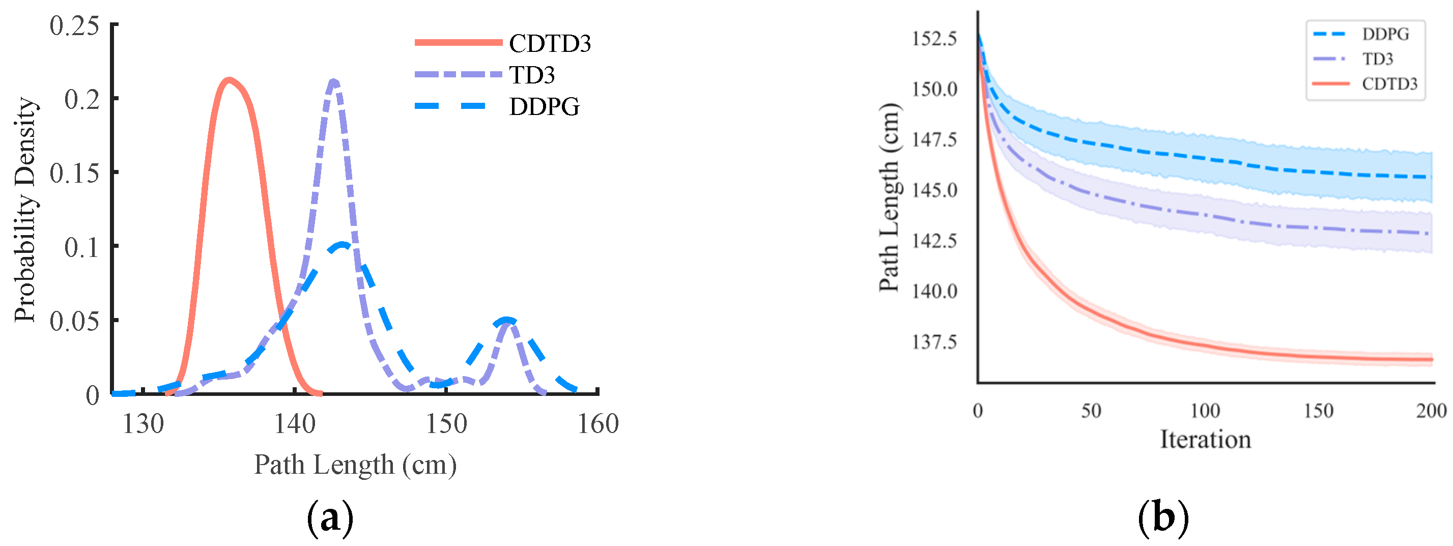
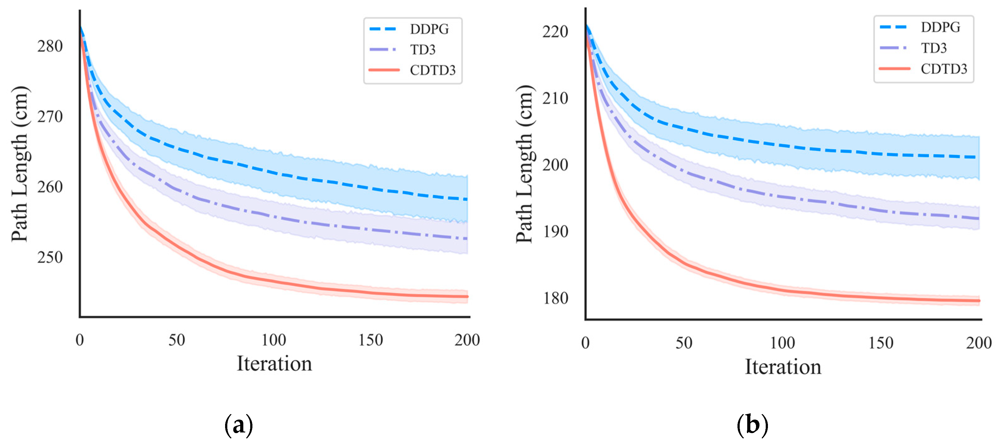
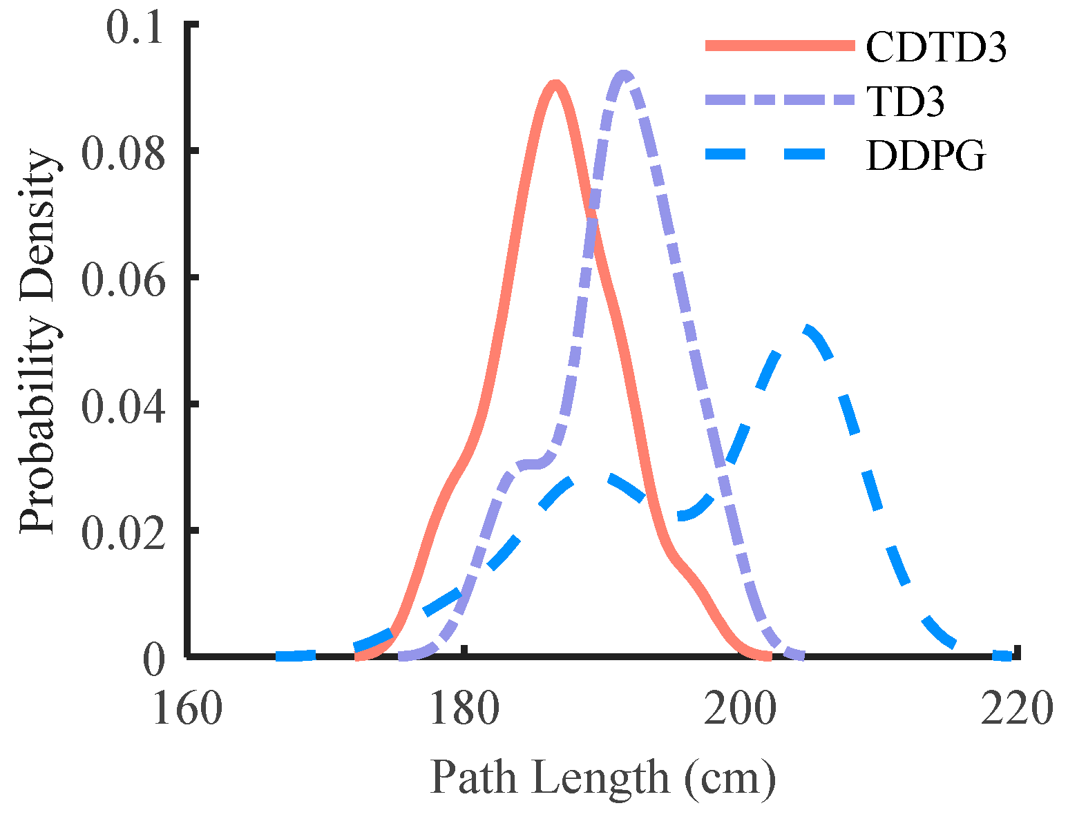
The results shown in Figure 5a represent the probability density. The x-axis represents the path length, while the y-axis represents the percentage of distribution. The curve represents the distribution of the path lengths from multiple experiments. From the probability density curve, it can be observed that, under the influence of CDTD3, the majority of results were concentrated in the region of the smaller path lengths. The distribution was relatively dense, and the final results exhibited less fluctuation, indicating a higher level of stability. The results of TD3 and DDPG were more dispersed and distributed in the region of larger path lengths. The relationship between the changes in path length obtained by the three algorithms is illustrated in Figure 5b. As the number of iteration steps increases, the path length undergoes continuous optimization and reduction., CDTD3 demonstrates superior ability to explore a more optimal path compared to TD3 and DDPG in most experimental cases, resulting in shorter path lengths and greater consistency with each optimization.

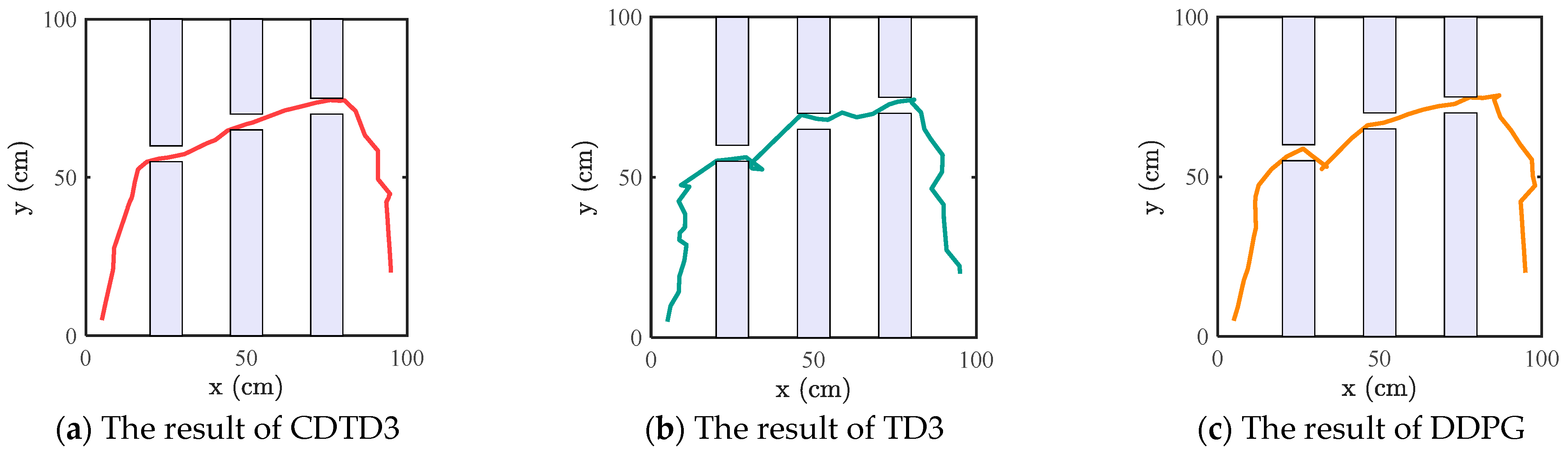
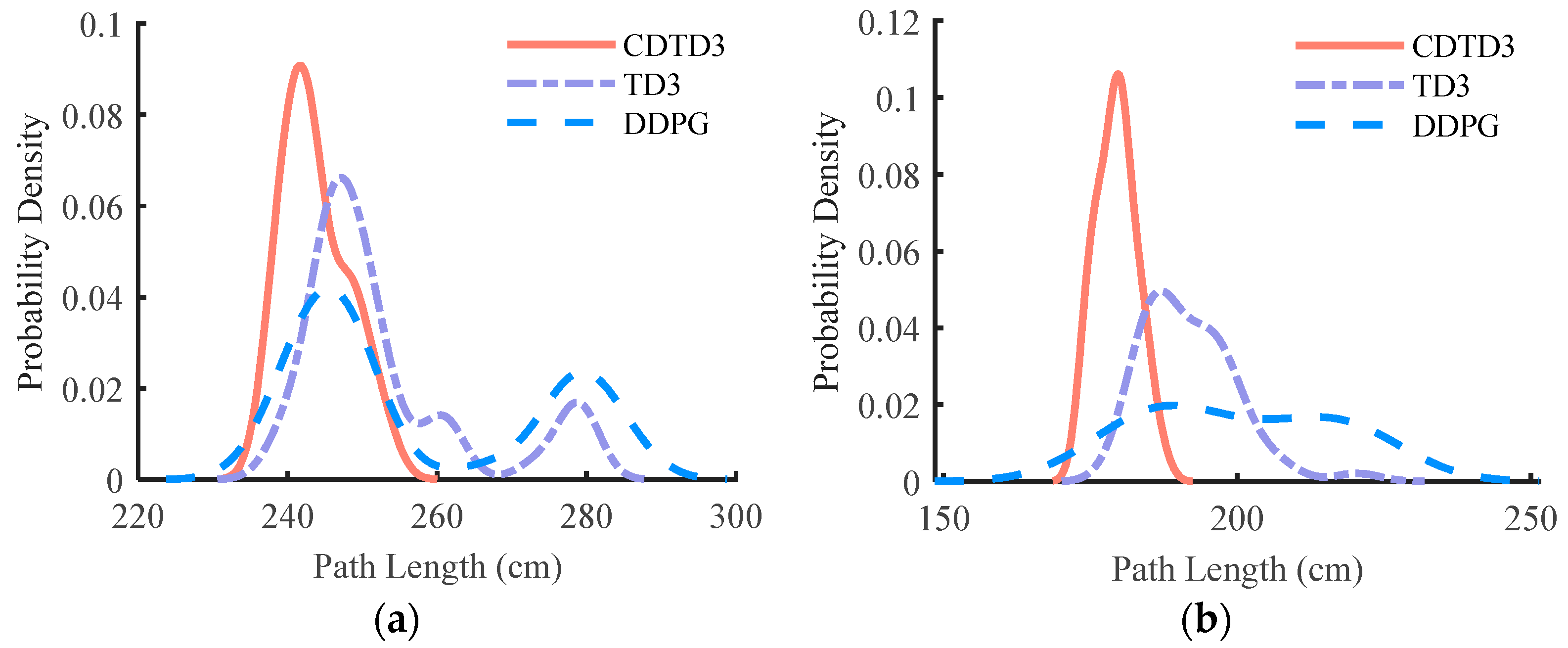
The simulations for the maze space and the narrow space environment as shown in Figure 6 and Figure 7 is designed, the lines represent the paths and the purple geometric objects represent obstacles. The starting point and obstacles were set differently. In the narrow space environment depicted in Figure 7, the distance between the two obstacles vertically was less than 10 cm. The obstacle avoidance path connecting the starting point and the target point needed to pass through all the narrow channels. The path explored by RRT* tended to be more winding; however, by using CDTD3 to optimize the path, continuously adjusting the intermediate waypoints, even in the case of a narrow space with a relatively singular path, the optimized path by CDTD3 still demonstrated advantages. It appeared more straight and shorter in the overall path. The probability density statistics of the path length in maze space and narrow space are illustrated in Figure 8, while Figure 9 depicts the changes in the path. Aligning with the outcomes observed in the complex obstacle space, CDTD3 outperformed in these two cases.

The simulation results in the three environments were analyzed. The mean and variance in

Table 1. Mean and variance statistics of path length in the 2D simulation environment.

Algorithm	Index	Complex Obstacle	Maze Space	Narrow Space
CDTD3	Mean (cm)	136.60	244.32	179.55
	Variance	2.59	20.51	12.39
TD3	Mean (cm)	142.81	252.56	191.88
	Variance	23.79	127.29	75.65
DDPG	Mean (cm)	145.62	258.12	201.08
	Variance	38.44	278.97	260.86

correspond to the outcomes of 100 experiments. The original path lengths were 154.1 cm, 284.7 cm, and 222.1 cm, respectively, while the path lengths optimized by CDTD3 were 136.6 cm, 244.4 cm, and 179.55 cm, respectively. The success rate of path iteration and the results of path reduction rate are presented in

Table 2. Optimization success rate and path reduction rate of the 2D simulation environment.

Algorithm	Index	Complex Obstacle	Maze Space	Narrow Space
CDTD3	Success rate	91.3%	87.3%	95.6%
	Reduction rate	11.4%	14.2%	19.14%
TD3	Success rate	88.2%	85.5%	98.7%
	Reduction rate	7.4%	10.2%	13.59%
DDPG	Success rate	76.2%	79.5%	86.8%
	Reduction rate	5.5%	73.2%	9.44%

, where the reduction rate represents the percentage reduction to the RRT* path length. The success rates of CDTD3 performing point-to-point tasks in the three environments were 91.3%, 87.3%, and 95.6%, respectively, which were better than those of TD3 and DDPG, owing to the random exploration mechanism of CDTD3 algorithm.

CDTD3 is combined with RRT* and RRT, respectively; and conducted 100 simulations in complex obstacle and maze environments. The settings of RRT remained consistent with those of RRT*, except for the inherent characteristics of their respective. The simulation results are shown in

Table 3. Results of CDTD3-RRT* and CDTD3-RRT in the 2D simulation environment.

Algorithm	Index	Complex Obstacle	Maze Space
CDTD3-RRT*	Mean (cm)	136.6	244.32
	Variance	2.59	20.51
	Reduction rate	11.4%	14.2%
CDTD3-RRT	Mean (cm)	154.9	258.92
	Variance	8.49	51.56
	Reduction rate	10.8%	19.3%

. Using CDTD3-RRT* could achieve a superior path due to the advantageous features offered by RRT*. This characteristic led to an improved initial path, resulting in a shorter final path. In the maze environment, the reduction rate of CDTD3-RRT was better than that of CDTD3-RRT*, but the final path length was not as good as that of CDTD3-RRT* since the path of the original RRT was longer than that of RRT*. Nevertheless, favorable outcomes can still be achieved using the proposed method.

In the complex obstacle space and maze space, CDTD3-RRT* was compared with two more advanced path planning methods, including the artificial potential field with informed RRT* (APF-IRRT*) [36], the adjustable probability and sampling area RRT algorithm (APS-RRT) [37].

Table 4. Comparison of the path planning in the 2D simulation environment.

Algorithm	Index	Complex Obstacle	Maze Space
CDTD3-RRT*	Mean (cm)	136.6	244.32
	Variance	2.59	20.51
APF-IRRT*	Mean (cm)	171.13	312.15
	Variance	200.33	316.21
APS-RRT	Mean (cm)	167.32	315.18
	Variance	191.35	322.69

presents the performance comparison of CDTD3-RRT* under 100 experiments. It can be seen that CDTD3-RRT* has significant advantages under the path length. Owing to the powerful sampling and search ability of RRT* and the optimization ability of CDTD3, APS-RRT and APF-IRRT* use limited exploration range operations in the two complex environments, which is not conducive to obtaining better paths.

4.2. Analysis of the 3D Simulation Environment

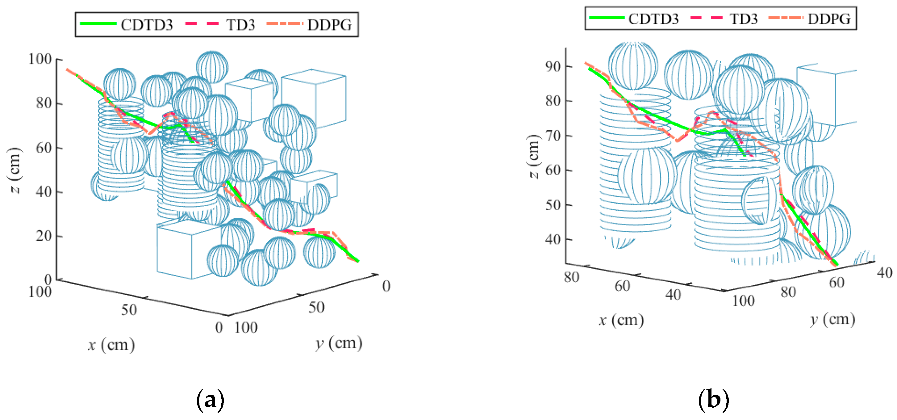
In order to verify the performance of the CDTD3-RRT* path planning method in 3D complex obstacle environments, a 3D space simulation environment was designed, with size of 100 (cm³). The environment is shown in Figure 10a, Figure 10b is locally enlarged, and multiple obstacles of different sizes and shapes were set up in the environment.

RRT* was first used for 5000 iterations with the starting position at (6, 6, 6) and the target position at (98, 96, 95). DRL were used to carry out 50 simulation experiments on the DRL-RRT*, each experiment was conducted under different random seeds, and each experiment had 400 iterations. The length of each point-to-point task was 400 steps.

The simulation results are shown in

Table 5. Results of the 3D complex obstacle space simulation.

Algorithm	Mean(cm)	Variance	Success Rate	Reduction Rate
CDTD3	186.61	20.09	94.35%	10.6%
TD3	191.23	20.21	91.78%	8.2%
DDPG	197.29	79.93	62.43%	4.4%

. The average path lengths for 50 repeated experiments were 186.61 cm, 191.23 cm, and 197.29 cm, respectively. Figure 11 shows the relationship between path length and algorithms. The random policy was added to the CDTD3 to further optimize the performance of the algorithm. In the 3D environment, CDTD3 consistently discovered shorter paths across multiple experiments, leading to reduced path length and higher success rates for D-P2P tasks.

5. Simulation and Experiment of Manipulator Path Planning

5.1. Evaluation Index of Path Planning

The accuracy and stability of path planning algorithms require certain indicators for evaluation. Typically, the root mean square error (RMSE) analysis method is employed to quantify the deviation between the desired value $x_i$ and actual value $y_i$ of the manipulator trajectories. The RMSE is expressed as follows:

$$RMSE=\sqrt{\frac{1}{n}{\displaystyle \sum _{i=1}^n{(x_i-y_i)}^2}}$$

(13)

The success rate of position deviation is used to measure the discrepancy between the actual target position and the set target position. The distance $d_i$ between the actual target $(x_i,y_i,z_i)$ and the set target $(\overline{x},\overline{y},\overline{z})$ is calculated as follows:

$$d_i=\sqrt{{(x_i-\overline{x})}^2+{(y_i-\overline{y})}^2+{(z_i-\overline{z})}^2}$$

(14)

The success rate of the position deviation in the experiment can be expressed by:

$$G=\frac{1}{N}{\displaystyle \sum _{i=1}^n{g}_i}$$

(15)

where $N$ is the number of experiments; $g_i\in \{0,1\}$; if $d_i<\phi$, then $g_i=1$, otherwise $g_i=0$. $\phi$ is a threshold that can be used to measure the relationship between $d_i$ and $G$.

5.2. Experiment and Simulation Research on the Application of Manipulator Path Planning

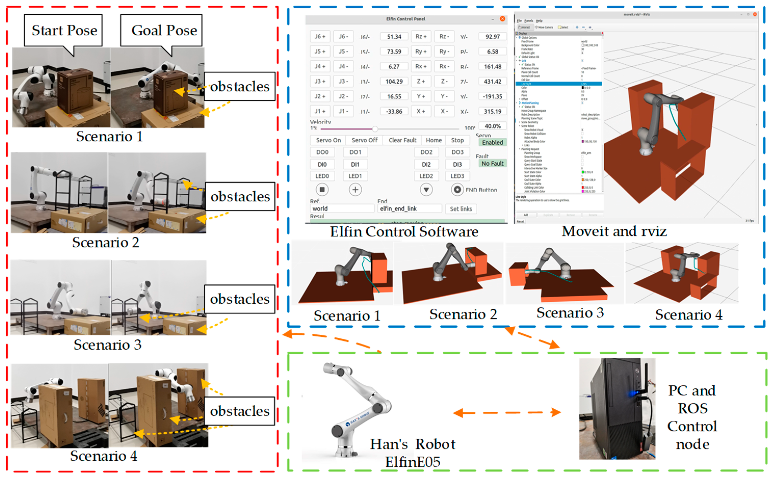
A manipulator experimental platform was established as shown in Figure 12 to verify the feasibility of the proposed method in the practical manipulator. The hardware of the experimental platform included the 6-DOF manipulator Han’s Robot Elfin E05, the supporting tools and the computer were equipped with the Ubuntu20 operating system. ROS Noetic MoveIt 1 is an open-source robotic motion planning framework for robot motion planning and control. It provides collision checking and control functionalities, integrating collision detection libraries such as the Flexible Collision Library (FCL), which is used to detect collisions between the robot and the environment or other objects.

Manipulator simulations were conducted to test the path planning. The use of the simulation environment allowed us to perform multiple experiments under different scenarios, conditions, and parameter settings to ensure the rationality and feasibility of the planned paths, reducing the wear and tear on the manipulator in real-world experiments. The simulation environment shown in Figure 12 was established for the obstacle avoidance path planning task of the manipulator using Rviz and MoveIt1. The simulation environment consisted of four different obstacle environments and various starting positions and target positions, all of which closely resembled real-world scenarios.

In the CDTD3 algorithm, $\lambda =0.1$, $c=1$, and $i=100$. A total of 100 simulation experiments were conducted on the manipulator. The average length of the executed path in the joint space and the success rate of planning execution results are presented in

Table 6. The results of manipulator simulation.

Algorithm	Index	Scenario 1	Scenario 2	Scenario 3	Scenario 4
CDTD3-RRT*	Mean (cm)	146.3	56.1	108.7	90.7
	Success rate	98%	86%	92%	100%
TD3-RRT*	Mean (cm)	149.7	58.8	108.5	94.1
	Success rate	99%	85%	92%	100%
DDPG-RRT*	Mean (cm)	151.0	58.9	109.4	91.1
	Success rate	98%	87%	93%	100%

, the threshold $\phi$ in the experiment was 5 (cm). According to the results in Table 6, the paths generated by CDTD3-RRT* had a good performance on different tasks, with shorter paths after planning and execution. In Scenario 3, where the task was relatively simple, the results of CDTD3 and TD3 were similar. Moreover, under four different tasks, three algorithms had a higher success rate in path planning. In the four scenarios, the paths obtained through the CDTD3-RRT* had a better length compared to those obtained through RRT*. The path reduction rates were 11.1%, 31%, 9.0%, and 20.4%, respectively.

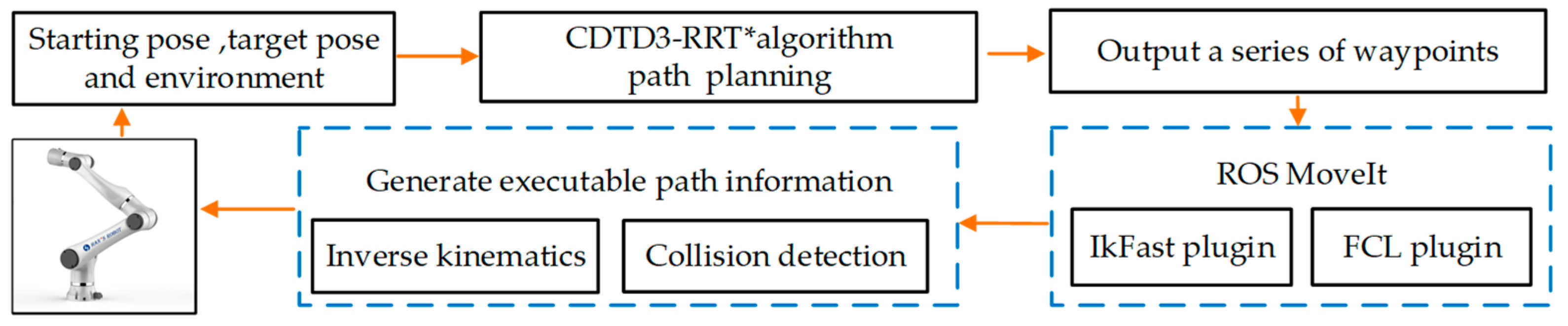
The manipulator experimental platform is shown in Figure 12. The process of obtaining the executable path of the manipulator is shown in Figure 13. When conducting path planning experiments on manipulator, given the starting pose, target pose and obstacle information. CDTD3-RRT* is first used to compute a collision-free path based on the environment. Then, the inverse kinematics solution and obstacle avoidance detection were performed using the motion planning method computed cartesian path in MoveIt1, which integrates IKFast and FCL plugin. Thus, the executable path of the joint space was calculated, and information such as joint variables required for the operation of the manipulator was output. After obtaining the executable path information, it was sent to Elfin E05 for execution. CDTD3-RRT* was tested multiple times to verify the performance in different targets. During the operation of the manipulator, a ROS node was utilized to collect real-time joint parameters, which were recorded in the file for further analysis.

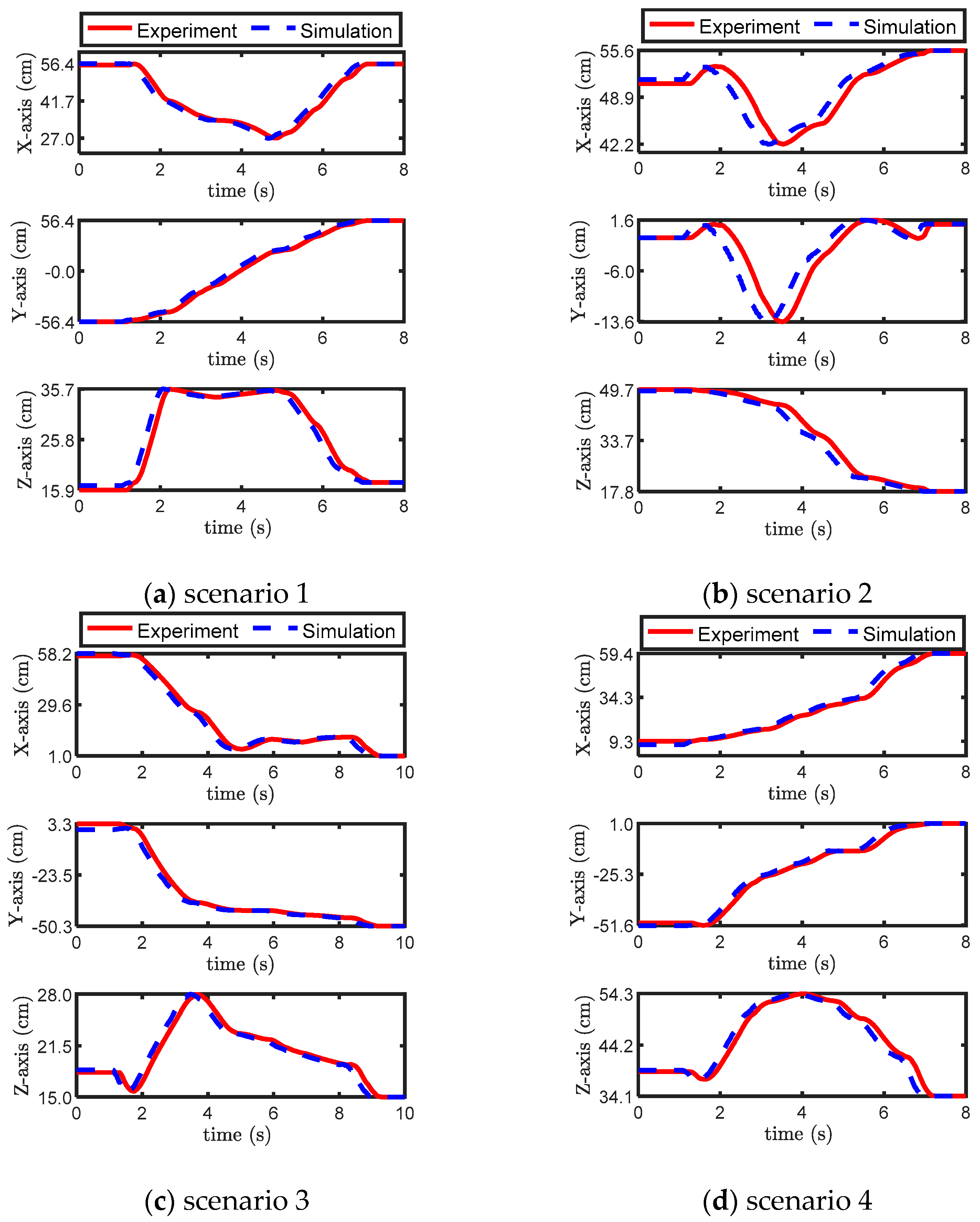
The comparison between the manipulator’s end path and the planned trajectory is illustrated in Figure 14. To accurately analyze the error, the trajectory was decomposed into three axes: the x-axis, y-axis, and z-axis. Although there were errors in each axis direction of the manipulator’s end path, the error was in a small range, which was consistent with the deviation between the actual experiment and the planned path.

According to Equation (13), the RMSE between the end effector trajectories of the four targets and the planned trajectory is calculated, including the results in three axes directions. The results shown in

Table 7. The RMSE for each direction at the manipulator’s end position.

RMSE	Scenario 1	Scenario 2	Scenario 3	Scenario 4
x-axis (cm)	2.1	3.2	2.6	1.4
y-axis (cm)	1.8	2.7	2.8	1.7
z-axis (cm)	3.1	1.3	1.7	3.1

are the average of 20 planning experiments. The results show that the proposed algorithm can complete the experimental task of manipulator path planning with high accuracy, and the error between the actual trajectory and the planned trajectory is acceptable. The actual trajectory of the manipulator during operation may have deviations from the planned results due to the inherent instability of the manipulator and the influence of prior information such as environment modeling and motion models in path planning. However, the small magnitude of the errors demonstrates that the algorithm is capable of effectively solving the path planning problem for the manipulator and achieves good effects in various tasks under different scenarios.

6. Conclusions

Based on the RRT*, this paper introduces the DRL to carry out path planning for the manipulator and seek an optimal path. To enhance the exploration ability of the TD3, an improved method called CDTD3 is proposed. Through simulation verification, this method can effectively improve the insufficient exploration in the early stage of the TD3. Moreover, a path planning method DRL-RRT* was designed that combines the random sampling mechanism of the RRT* and the experience replay mechanism of DRL.

Path planning simulations were designed to validate the optimization ability of the proposed CDTD3-RRT* on the original path. The simulation results demonstrated that in three 2D environments, the original RRT* path achieved a reduction rate of 11.4%, 14.2%, and 19.14%, respectively. The reduction rate in the 3D complex obstacle environment was 10.6%. In addition, the CDTD3 demonstrated a significant improvement in the success rate of iterative optimization and reduction rate compared with the TD3 and DDPG. Finally, an experimental platform for manipulator was established, and the application of path planning methods in obstacle avoidance path planning tasks was analyzed. The results demonstrate that the path length of CDTD3-RRT* was better than that of TD3-RRT*, and DDPG-RRT* in multiple experiments. In the four experimental scenarios, the paths obtained through the CDTD3-RRT* path planning method were more optimal in terms of length compared to the paths obtained through RRT*. The reduction rates of the paths in the four scenarios were 11.1%, 31%, 9.0%, and 20.4%, respectively, and the end path error of the manipulator conformed to the results of planning and actual execution.

References

- Lao, C.; Li, P.; Feng, Y. Path Planning of Greenhouse Robot Based on Fusion of Improved A* Algorithm and Dynamic Window Approach. Nongye Jixie Xuebao/Trans. Chin. Soc. Agric. Mach. 2021, 52, 14–22. [Google Scholar]
- Kavraki, L.E.; Svestka, P.; Latombe, J.C.; Overmars, M.H. Probabilistic roadmaps for path planning in high-dimensional configuration spaces. IEEE Trans. Robot. Autom. 1996, 12, 566–580. [Google Scholar] [CrossRef]
- Qi, J.; Yang, H.; Sun, H. MOD-RRT*: A Sampling-Based Algorithm for Robot Path Planning in Dynamic Environment. IEEE Trans. Ind. Electron. 2021, 68, 7244–7251. [Google Scholar] [CrossRef]
- Viseras, A.; Shutin, D.; Merino, L. Online information gathering using sampling-based planners and GPs: An information theoretic approach. In Proceedings of the 2017 IEEE/RSJ International Conference on Intelligent Robots and Systems (IROS), Vancouver, BC, Canada, 24–28 September 2017; pp. 123–130. [Google Scholar]
- Gammell, J.D.; Srinivasa, S.S.; Barfoot, T.D. Informed RRT*: Optimal Sampling-based Path Planning Focused via Direct Sampling of an Admissible Ellipsoidal Heuristic. In Proceedings of the 2014 IEEE/RSJ International Conference on Intelligent Robots and Systems (IROS), Chicago, IL, USA, 14–18 September 2014; pp. 2997–3004. [Google Scholar]
- Islam, F.; Nasir, J.; Malik, U.; Ayaz, Y.; Hasan, O. RRT*-Smart: Rapid convergence implementation of RRT* towards optimal solution. In Proceedings of the 2012 IEEE International Conference on Mechatronics and Automation (ICMA), Chengdu, China, 5–8 August 2012; pp. 1651–1656. [Google Scholar]
- Lv, H.; Zeng, D.; Li, X. Based on GMM-RRT* Algorithm for Path Planning Picking Kiwifruit Manipulator. In Proceedings of the 2023 42nd Chinese Control Conference (CCC), Tianjin, China, 24–26 July 2023; pp. 4255–4260. [Google Scholar]
- Xinyu, W.; Xiaojuan, L.; Yong, G.; Jiadong, S.; Rui, W. Bidirectional Potential Guided RRT* for Motion Planning. IEEE Access 2019, 7, 95046–95057. [Google Scholar] [CrossRef]
- Naderi, K.; Rajamäki, J.; Hämäläinen, P. RT-RRT*: A real-time path planning algorithm based on RRT*. In Proceedings of the Proceedings of the 8th ACM SIGGRAPH Conference on Motion in Games, New York, NY, USA, 16 November 2015; pp. 113–118. [Google Scholar]
- Mnih, V.; Kavukcuoglu, K.; Silver, D.; Rusu, A.A.; Veness, J.; Bellemare, M.G.; Graves, A.; Riedmiller, M.; Fidjeland, A.K.; Ostrovski, G.; et al. Human-level control through deep reinforcement learning. Nature 2015, 518, 529–533. [Google Scholar] [CrossRef] [PubMed]
- Dabbaghjamanesh, M.; Moeini, A.; Kavousi-Fard, A. Reinforcement Learning-Based Load Forecasting of Electric Vehicle Charging Station Using Q-Learning Technique. IEEE Trans. Ind. Inform. 2021, 17, 4229–4237. [Google Scholar] [CrossRef]
- Hao, Y.; Chen, M.; Gharavi, H.; Zhang, Y.; Hwang, K. Deep Reinforcement Learning for Edge Service Placement in Softwarized Industrial Cyber-Physical System. IEEE Trans. Ind. Inform. 2021, 17, 5552–5561. [Google Scholar] [CrossRef] [PubMed]
- Shi, H.; Shi, L.; Xu, M.; Hwang, K.S. End-to-End Navigation Strategy with Deep Reinforcement Learning for Mobile Robots. IEEE Trans. Ind. Inform. 2020, 16, 2393–2402. [Google Scholar] [CrossRef]
- Bae, H.; Kim, G.; Kim, J.; Qian, D.; Lee, S. Multi-Robot Path Planning Method Using Reinforcement Learning. Appl. Sci. 2019, 9, 3057. [Google Scholar] [CrossRef]
- Lv, L.; Zhang, S.; Ding, D.; Wang, Y. Path Planning via an Improved DQN-Based Learning Policy. IEEE Access 2019, 7, 67319–67330. [Google Scholar] [CrossRef]
- Lillicrap, T.P.; Hunt, J.J.; Pritzel, A.; Heess, N.; Erez, T.; Tassa, Y.; Silver, D.; Wierstra, D. Continuous control with deep reinforcement learning. arXiv 2015, arXiv:1509.02971. [Google Scholar]
- Andrychowicz, M.; Wolski, F.; Ray, A.; Schneider, J.; Fong, R.; Welinder, P.; McGrew, B.; Tobin, J.; Abbeel, P.; Zaremba, W. Hindsight Experience Replay. arXiv 2017, arXiv:1707.01495. [Google Scholar]
- Gu, S.; Holly, E.; Lillicrap, T.; Levine, S. Deep reinforcement learning for robotic manipulation with asynchronous off-policy updates. In Proceedings of the 2017 IEEE International Conference on Robotics and Automation (ICRA), Singapore, 29 May–3 June 2017; pp. 3389–3396. [Google Scholar]
- Lin, G.; Zhu, L.; Li, J.; Zou, X.; Tang, Y. Collision-free path planning for a guava-harvesting robot based on recurrent deep reinforcement learning. Comput. Electron. Agric. 2021, 188, 106350. [Google Scholar] [CrossRef]
- Yang, Y.; Ni, Z.; Gao, M.; Zhang, J.; Tao, D. Collaborative Pushing and Grasping of Tightly Stacked Objects via Deep Reinforcement Learning. IEEE/CAA J. Autom. Sin. 2022, 9, 135–145. [Google Scholar] [CrossRef]
- Li, X.; Liu, H.; Dong, M. A General Framework of Motion Planning for Redundant Robot Manipulator Based on Deep Reinforcement Learning. IEEE Trans. Ind. Inform. 2022, 18, 5253–5263. [Google Scholar] [CrossRef]
- Kim, M.; Han, D.-K.; Park, J.-H.; Kim, J.-S. Motion Planning of Robot Manipulators for a Smoother Path Using a Twin Delayed Deep Deterministic Policy Gradient with Hindsight Experience Replay. Appl. Sci. 2020, 10, 575. [Google Scholar] [CrossRef]
- Fujimoto, S.; van Hoof, H.; Meger, D. Addressing Function Approximation Error in Actor-Critic Methods. arXiv 2018, arXiv:1802.09477. [Google Scholar]
- Pan, L.; Cai, Q.; Huang, L. Softmax Deep Double Deterministic Policy Gradients. arXiv 2020, arXiv:2010.09177. [Google Scholar]
- Maoudj, A.; Hentout, A. Optimal path planning approach based on Q-learning algorithm for mobile robots. Appl. Soft Comput. 2020, 97, 106796. [Google Scholar] [CrossRef]
- Chiang, H.T.L.; Faust, A.; Fiser, M.; Francis, A. Learning Navigation Behaviors End-to-End with AutoRL. IEEE Robot. Autom. Lett. 2019, 4, 2007–2014. [Google Scholar] [CrossRef]
- Li, H.; Zhang, Q.; Zhao, D. Deep Reinforcement Learning-Based Automatic Exploration for Navigation in Unknown Environment. IEEE Trans. Neural Netw. Learn. Syst. 2020, 31, 2064–2076. [Google Scholar] [CrossRef]
- Francis, A.; Faust, A.; Chiang, H.T.L.; Hsu, J.; Kew, J.C.; Fiser, M.; Lee, T.W.E. Long-Range Indoor Navigation with PRM-RL. IEEE Trans. Robot. 2020, 36, 1115–1134. [Google Scholar] [CrossRef]
- Kontoudis, G.P.; Vamvoudakis, K.G. Kinodynamic Motion Planning with Continuous-Time Q-Learning: An Online, Model-Free, and Safe Navigation Framework. IEEE Trans. Neural Netw. Learn. Syst. 2019, 30, 3803–3817. [Google Scholar] [CrossRef]
- Gao, J.; Ye, W.; Guo, J.; Li, Z. Deep Reinforcement Learning for Indoor Mobile Robot Path Planning. Sensors 2020, 20, 5493. [Google Scholar] [CrossRef]
- Florensa, C.; Held, D.; Wulfmeier, M.; Zhang, M.; Abbeel, P. Reverse Curriculum Generation for Reinforcement Learning. arXiv 2017, arXiv:1707.05300. [Google Scholar]
- Chiang, H.T.L.; Hsu, J.; Fiser, M.; Tapia, L.; Faust, A. RL-RRT: Kinodynamic Motion Planning via Learning Reachability Estimators from RL Policies. IEEE Robot. Autom. Lett. 2019, 4, 4298–4305. [Google Scholar] [CrossRef]
- Uther, W. Markov Decision Processes. In Encyclopedia of Machine Learning and Data Mining; Sammut, C., Webb, G.I., Eds.; Springer: Boston, MA, USA, 2017; pp. 793–798. [Google Scholar]
- Haarnoja, T.; Zhou, A.; Abbeel, P.; Levine, S. Soft Actor-Critic: Off-Policy Maximum Entropy Deep Reinforcement Learning with a Stochastic Actor. arXiv 2018, arXiv:1801.01290. [Google Scholar]
- Silver, D.; Lever, G.; Heess, N.; Degris, T.; Wierstra, D.; Riedmiller, M. Deterministic Policy Gradient Algorithms. In Proceedings of the 31st International Conference on Machine Learning (ICML), Beijing, China, 21–26 June 2014; pp. 387–395. [Google Scholar]
- Wu, D.; Wei, L.; Wang, G.; Tian, L.; Dai, G. APF-IRRT*: An Improved Informed Rapidly-Exploring Random Trees-Star Algorithm by Introducing Artificial Potential Field Method for Mobile Robot Path Planning. Appl. Sci. 2022, 12, 10905. [Google Scholar] [CrossRef]
- Li, X.; Tong, Y. Path Planning of a Mobile Robot Based on the Improved RRT Algorithm. Appl. Sci. 2024, 14, 25. [Google Scholar] [CrossRef]
Figure 1.
Flowchart of the CDTD3 algorithm.
Figure 2.
Simulation results of CDTD3 in MuJoCo: (a) Walker2d-v4, (b) Ant-v4, and (c) Hopper-v4.
Figure 3.
Flowchart of the DRL-RRT* path planning algorithm.
Figure 4.
Simulation environment for a complex obstacle space.
Figure 5.
Simulation results of the 2D complex obstacle space. (a) The probability density of path length. (b) Diagram of the length variation during the path optimization process.
Figure 6.
Simulation environment for the maze space.
Figure 7.
Simulation environment for the narrow space.
Figure 8.
Probability density results of path length. (a) The results of the maze space. (b) The results of the narrow space.
Figure 9.
Diagram of the relationship between path length change and the algorithm. (a) The results of the maze space. (b) The results of the narrow space.
Figure 10.
3D complex obstacle environment: (a) complete 3D environment and (b) locally enlarged view of the 3D environment.
Figure 11.
Probability density of the 3D complex obstacle space simulation.
Figure 12.
The experimental platform for the manipulator.
Figure 13.
The process of generating the executable path information.
Figure 14.
The end trajectory of the manipulator.