A Phase Correction Model for Fourier Transform Spectroscopy

Abstract

In Fourier transform spectroscopy (FTS), the conventional Mertz method is commonly used to correct phase errors of recovered spectra, but it performs poorly in correcting nonlinear phase errors. This paper proposes a phase correlation method–all-pass filter (PCM-APF) model to correct phase errors. In this model, the proposed improved phase correlation method can correct linear phase errors, and all-pass filters are applied to correct the residual nonlinear phase errors. The optimization algorithm for the digital all-pass filters employs an improved algorithm which combines the subtraction-average-based optimizer (SABO) and the golden sine algorithm (Gold-SA). The proposed PCM-APF model demonstrates high correction precision, and the optimization algorithm for the filters converges faster than traditional intelligent optimization algorithms.

1. Introduction

In recent years, Fourier transform spectroscopy (FTS) has undergone significant development. It has been widely applied in various disciplines and fields such as analytical chemistry [1], hyperspectral imaging [2], frequency comb spectroscopy [3], earth sciences [4], ultrafast spectrometry [5], and so on. Traditional FTS provides interference data of spectra, requiring further processing of interferograms to obtain the desired spectral information. This includes operations such as apodization, phase correction, and fast Fourier transform, among others.

In FTS, phase correction is crucial for eliminating phase errors in the recovered spectra. Several methods, including the double-sided interferogram method, the convolution method, and the Mertz method [6,7,8], can be employed. The double-sided interferogram method calculates all data points in a double-sided interferogram, completely eliminating phase errors. However, it is highly sensitive to noise. Therefore, in the recovery of spectra, single-sided interferogram methods are commonly employed. Among them, the Mertz method and the convolution method are the most commonly used. The Mertz method is easy to compute, but it may not be as effective in correcting nonlinear phase errors. On the other hand, the convolution method can correct nonlinear phase errors, but when the phase error is substantial it may require multiple convolution operations, resulting in increased computational complexity and instability [9,10].

Using the phase correlation method to correct phase errors in FTS was first proposed by Wang in 2011 [11]. This method can reach high precision in linear phase correction. The phase correlation method involves time delay calculation of two channels of interferograms to correct linear phase errors.

A phase correction method based on all-pass filters was initially proposed by Furstenberg in 2005 [12] and improved by Li in 2015 [13], who introduced an all-pass filter–delayer–phaser (ADP) model for phase correction. The all-pass filter has a magnitude–frequency response of 1 across the entire frequency range. Therefore, it is used as a filter to correct residual phase errors in the interferogram. In this way, the amplitude of the output spectra remains stable, and only the phase is modified [12,13,14].

This paper presents a practical phase correction model called the PCM-APF model. The proposed model shows high correction accuracy and efficiency, combining the phase correlation method with all-pass filters. For filter optimization algorithm, we adopt an improved gold sine-subtraction average-based optimizer (GS-SABO) algorithm, combining the subtraction average-based optimizer (SABO) and the golden sine algorithm (Gold-SA) to optimize the parameter settings of the filters [15,16]. The PCM-APF model uses an improved phase correlation method to correct linear phase errors, while all-pass filters are used to correct the remaining phase errors.

2. Phase Correction by the Mertz Method

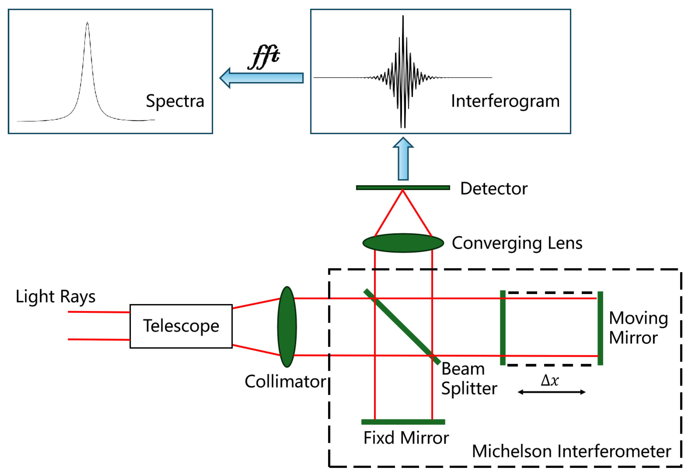
Figure 1 depicts a common imaging FTS system based on a Michelson interferometer. In FTS, the incident beam undergoes modulation within the interferometer, generating two outgoing beams with varying optical path differences. These two beams interfere on the image plane, creating interferograms. The collected interferogram and the spectra of the incident beam are related through Fourier transform:

$$B\left(\nu \right)={\int }_{-\infty }^{+\infty }I(\Delta )e^{-j2\pi \nu \Delta }d\Delta$$

(1)

$B\left(\nu \right)$ is the recovered spectrum from interferogram $I(\Delta )$, $\nu$ is the wavenumber, and $\Delta$ is the optical path difference.

In the Mertz method, small double-sided interferograms near the zero-path difference (ZPD) point, with high interference signal intensity and SNR (signal-to-noise ratio), are usually used to calculate the error phase:

$$\phi =arctan\frac{Im\left(\nu \right)}{Re\left(\nu \right)}$$

(2)

Im ($\nu$) and Re ($\nu$) are the imaginary and real parts of the spectra recovered by a small double-sided interferogram.

In this method, we assume that the error phase is a slowly varying function with respect to the wavenumber. Therefore, the small double-sided interferograms can be interpolated to the desired number of data points, which is used to guide the phase correction. The correction formula is as follows:

$$S\left(\nu \right)=R\left(\nu \right)cos\left(\phi \right(\nu \left)\right)+I\left(\nu \right)sin\left(\phi \right(\nu \left)\right)$$

(3)

R($\nu$) and I($\nu$) represent the real and imaginary parts of the original recovered spectra, respectively. $\phi \left(\nu \right)$ represents the error phase obtained from the small double-sided interferograms and S($\nu$) represents the spectra corrected by the Mertz method [9].

In sampling of interferograms, it is challenging to precisely sample the ZPD position. If the sampled ZPD point is sampled after the real ZPD position with an offset of $\epsilon$, according to the displacement property of the Fourier transform, the corresponding phase error is $\phi \left(\nu \right)=\epsilon \nu$. However, from the study of Liu [17] we know that the collected interferograms are always finite, i.e., they cannot be infinitely long, and so, do not meet the ideal time-shift property of the Fourier transform, so the phase error caused by the zero-point drift will also have nonlinear components. At the same time, the general Fourier transform spectrometer system can also produce spectra with a nonlinear phase error due to the instrument line shape (ILS) of the spectrometer, caused by optical aberrations [18].

3. Phase Correlation Method

The proposed PCM-APF model first requires the correction of linear phase errors, primarily caused by the ZPD offset. In some scholars’ research, to determine the linear phase component, they often perform linear fitting of the phase curve. In [19], polynomial fitting is used for phase correction. However, it must be considered that the phase error curve calculated by the inverse tangent function may jump if there is nonlinear phase error [20]. It is obvious that we have to unwrap the phase error curve before we can use the linear fit in this case, which increases the uncertainty and potential computation in practice; so we use the phase correlation method.

The phase correlation method is one of the most commonly used techniques for signal time-delay estimation. By calculating the cross-correlation function of two signals and identifying the location of the maximum value of the function, we can find the time delay which is equal to the distance in the x-axis between the maximum value point and the zero point [21].

In the PCM method proposed in [11], a Hanning window is applied to the interferogram initially. Subsequently, data points of equal length on both sides of the sampled point with maximum interference intensity are taken as two signals. The phase correlation method is then employed to calculate the time delay between these two signals.

Differing from the PCM method, the PCM-APF model in this paper modifies the phase correlation method used. It is essential to understand that the application of the Hanning window in the PCM method serves a purpose distinct from apodization in FTS data processing. Its function is more akin to the general phase correlation method [21,22], aiming to enhance the SNR of the selected signals. Moreover, due to the inherent asymmetry of the interferogram caused by the error phase, applying a Hanning window may lead to increased errors in time-delay estimation.

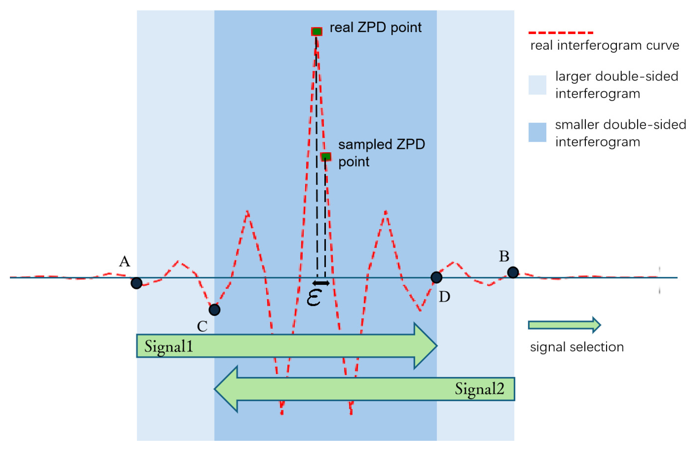
In the PCM-APF model proposed in this paper, we employ a new approach to selecting two signals. Let us assume that the collected interferogram only has ZPD-point drift, meaning it contains only linear phase error. Just like the Mertz method, we pre-define the number of data points for two small double-sided interferograms. Subsequently, we extract two small double-sided interferograms near the point of maximum interference intensity (sampled ZPD point). As illustrated in Figure 2, A and B represent the two endpoints of the larger double-sided interferogram, and similarly, C and D represent the two endpoints of the smaller double-sided interferogram. Then, we select the interference signal from point A to D as Signal1, and similarly, choose the interference signal from point B to C as Signal2. Additionally, since the selected signals are all in regions of the original interferogram with higher SNR, there is no need to apply a Hanning window to the selected signals.

Suppose the distance of the real ZPD position of the interferogram from the sampled ZPD position is $\epsilon$. By geometric considerations, it can be easily deduced that the theoretical time delay between Signal1 and Signal2 should be $2\epsilon$. In other words, by following the method described above to obtain the two interferometric signals, then using the previously mentioned phase correlation method to calculate the time delays of the two signals, and finally, dividing the result by 2, we can determine the linear ZPD-point drift of the interferogram.

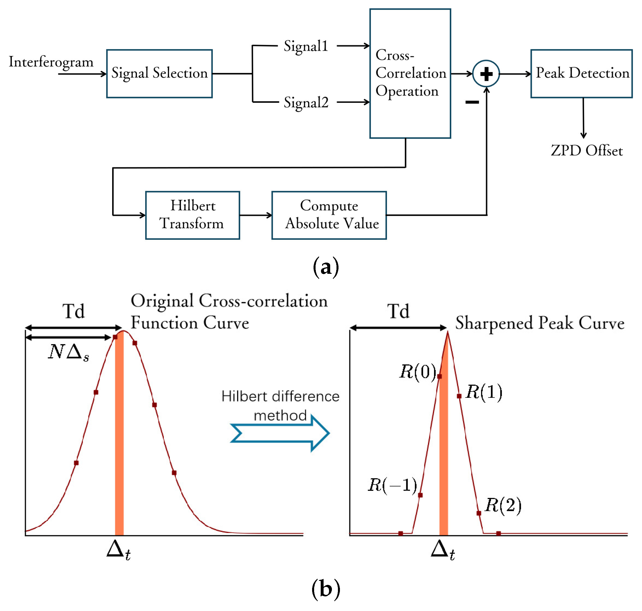
Since the method described above can only provide ZPD-point drift values in integer multiples of the sampling interval, so further sub-pixel peak estimation of the obtained cross-correlation function is needed. Wang [11] presented a fitting method for peak detection at peak positions [11,23]. In our PCM-APF model in this paper, we utilize the Hilbert difference method for sharpening the correlation peaks to achieve peak position determination. Figure 3a shows the basic process of ZPD offset calculation in proposed PCM-APF model.

The Hilbert difference method involves taking the difference between the absolute values of the cross-correlation function and its Hilbert transform. This process preserves values near the peaks while reducing the correlation of values outside the peaks. As a result, the sharpness of the main peak in the waveform of the received signal’s correlation function significantly increases [24]. After using the Hilbert difference method, the correlation peak becomes sharp and steep. Therefore, we assume that the points on the left and right sides near the peak have the same derivative values, but the point on the left is positive, while the one on the right is negative. As shown in Figure 3b, we define the maximum point and its adjacent two data points: $R(-1)$, $R\left(0\right)$, and $R\left(1\right)$ (supposing that $R\left(1\right)$>$R(-1)$). By geometric considerations, we can derive that

$${\Delta }_t=\frac{{\Delta }_s}{2}[1-\frac{\left|R\left(0\right)-R\left(1\right)\right|}{\left|R\left(0\right)-R(-1)\right|}]$$

(4)

where ${\Delta }_t$ is the distance between the sampled maximum point and the actual peak, and ${\Delta }_s$ is the sampling interval.

So the linear phase correction of this interferogram can be completed using the Mertz method. This involves processing the original interferogram using Equation (3), where the error phase is $\phi \left(\nu \right)=(N{\Delta }_s+{\Delta }_t)\nu$. $N{\Delta }_s$ represents the distance from the maximum point $R\left(0\right)$ to the y-axis, and its value is an integer multiple of the sampling interval.

4. All-Pass Filter and PCM-APF Model

4.1. Digital All-Pass Filter

Filters with amplitude responses that remain constant across the entire frequency band are called all-pass filters. An all-pass filter is an infinite impulse response (IIR) filter, and its system transfer function can be written in fractional form as follows:

$$\begin{array}{c}H\left(z\right)=\frac{a_N+a_{N-1}{z}^{-1}+a_{N-2}{z}^{-2}+\cdots +1z^{-N}}{1+a_1{z}^{-1}+a_2{z}^{-2}+\cdots +a_N{z}^{-N}}=\frac{z^{-N}Q\left(z^{-1}\right)}{Q\left(z\right)}\end{array}$$

(5)

where $Q\left(z\right)=1+a_1{z}^{-1}+a_2{z}^{-2}+\cdots +a_N{z}^{-N}$. We can further determine the zeros and poles of the all-pass filter:

$$H\left(z\right)=\frac{z^{-N}Q\left(z^{-1}\right)}{Q\left(z\right)}=\prod _{i=1}^N\frac{z^{-1}-p_i^{\ast }}{1-p_i{z}^{-1}}=\prod _{i=1}^N\frac{-p_i^{\ast }\left[z-{\left(\frac{1}{p_i}\right)}^{\ast }\right]}{z-p_i}$$

(6)

Obviously, $p_i$ and ${(1/p_i)}^{\ast }$ are a set of zeros and poles of the filter, which are conjugated to each other.

Based on previous research, we can infer that the phase response of an all-pass filter is

$$\theta \left(\omega \right)=-N\omega -2argQ\left(e^{i\omega }\right)$$

(7)

where the arg function represents the phase angle calculation using the arctan method, similar to Equation (2) [12,13].

4.2. The PCM-APF Model

The correction results of the sub-pixel phase correlation method still contains residual nonlinear phase errors. To effectively eliminate these residual errors, the use of an all-pass filter is well suited. The residual error is still calculated using the arctan function:

$${\theta }_{res}\left(\omega \right)=arctan\frac{Im\left(B^{\prime }\left(\omega \right)\right)}{Re\left(B^{\prime }\left(\omega \right)\right)}$$

(8)

where ${\theta }_{res}$ represents the nonlinear residual phase error, and $B^{\prime }\left(\omega \right)$ is the spectrum corrected after the sub-pixel phase correlation correction step. Here, $\omega$ is not the wavenumber but represents the normalized frequency, which ranges from 0 to $\pi$ radians/s, where $\pi$ radians/s corresponds to the Nyquist frequency $v_{max}$. The relationship between normalized frequency $\omega$ and wavenumber $\nu$ is as follows:

$$\omega =\pi \frac{\nu }{{\nu }_{max}}$$

(9)

Since a stable all-pass filter only generates negative phase responses, so the interferogram needs to pass through a delay line before applying the filter. This introduces a linear phase component, ensuring that the residual phase error curve values are all positive [14]. Thus, the final output error phase is

$${\theta }_{out}\left(\omega \right)={\theta }_{res}\left(\omega \right)+N_{\mathit{shift}}\omega -N\omega -2argQ\left(e^{i\omega }\right)$$

(10)

The value of the order N of the all-pass filter should depend on the smoothness of the error phase curve. N also depends on the magnitude of the residual phase error we expect for the corrected spectra. For a 3–10 degree error and a typical interferogram resulting from an absorption experiment on a rapid-scan FTIR, N = 9 will suffice [12]. In the proposed PCM-APF model, the value of N will be smaller because the interferogram is “pre-processed” by the phase correlation method before passing through the all-pass filter, in which most of the linear phase errors are removed.

We aim for a smaller value of ${\theta }_{out}$. So for an Nth-order all-pass filter, we establish an error function concerning the filter parameters and the delay order $N_{shift}$, with the expectation that the error function reaches its minimum value:

$$E\left(N_{shift},a_1,a_2,\cdots ,a_N\right)=\underset{{\omega }_a\le \omega \le {\omega }_b}{max}\left({\theta }_{out}\left(\omega \right)\right)$$

(11)

where ${\omega }_a$ and ${\omega }_b$ represent the upper and lower limits of the normalized frequencies.

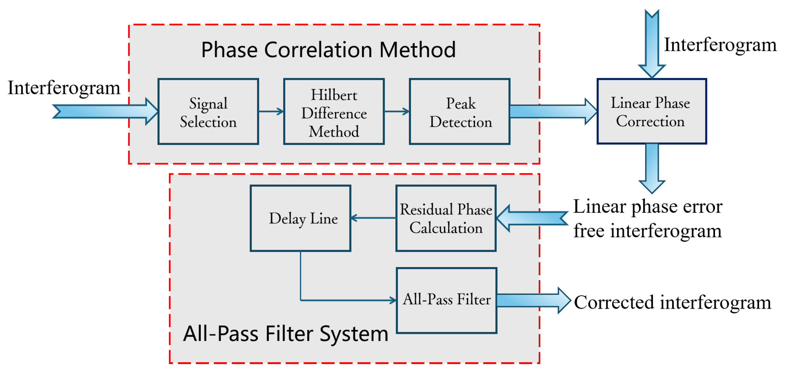
So the whole PCM-APF model for phase correction is as shown in Figure 4.

4.3. Filter Parameter Optimization Strategy

This paper uses an evolutionary algorithm to optimize Equation (11), employing a novel GS-SABO algorithm and population initialization strategies. This optimization method has a straightforward computational principle, fast convergence, and, in many engineering problems, performs better than traditional approaches like particle swarm optimization (PSO) [25].

4.3.1. SABO Algorithm

SABO is a new meta-heuristic algorithm developed by Trojovský in 2023 [15], and like most smart algorithms, it is also necessary to initialize and define a population in SABO, usually using a random function. SABO employs the arithmetic average position of all individuals in the population to update the positions of all individuals in the population. SABO accomplishes this using a specific operation, denoted as “$-v$”, where “$A-vB$” means individual B subtracts v from individual A. Its definition is as follows:

$$A-vB=sign(F\left(A\right)-F\left(B\right))(A-\overrightarrow{v}\ast B)$$

(12)

where $sign$ represents the sign function; F(A) and F(B) represent the fitness values of individuals A and B; $\overrightarrow{v}$ is a random vector with the same dimensions as the individual, where each dimension’s size is randomly chosen from the set $\{1,2\}$; and “∗” denotes the Hadamard product of two vectors.

In SABO, the displacement of any individual $X_i$ in the search space is calculated as the arithmetic average of the v-subtractions of other individuals $X_j$ relative to $X_i$. Therefore, the new position of each individual is calculated using the following formula:

$$X_i^{new}=X_i+{\overrightarrow{r}}_i\ast \frac{1}{N}\sum _{j=1}^N\left(X_i-v{X}_j\right),i=1,2,\dots ,N$$

(13)

where $\overrightarrow{r}$ is a random vector with the same dimensions as an individual, and N is the total number of individuals. $X_i^{new}$ represents the updated new position, which replaces the original position if it is better; otherwise, the original position is retained [15]:

$$X_i=\left\{\begin{array}{cc}{X}_i^{new},& F_i^{new}<F_i\\ X_i,& else\end{array}\right.$$

(14)

4.3.2. Population Initialization and Improvement Scheme

A population with good diversity in the initial stage can significantly improve the algorithm’s search efficiency. Randomly initializing individuals in the search space for the initial population can lead to poor diversity. Furthermore, since there is no prior knowledge about the global optimal solution for the optimization problem, it is essential to distribute individuals as uniformly as possible in the search space during population initialization [26].

Using chaos to generate the initial population can provide good diversity. The basic idea is to map the optimization variables to the value range within the chaos variable space using mapping rules, and then, linearly transform the obtained optimization solution back to the optimization space. There are several models for generating chaotic sequences, including logistic mapping, Chebyshev mapping, cubic mapping, ICMIC mapping, neuron mapping, sine mapping, and others [27,28]. In this paper, we use logistic mapping:

$$Y_{k+1}=4Y_k\left(1-Y_k\right)$$

(15)

Additionally, to accelerate the convergence speed of population evolution, researchers have introduced the concept of reverse learning. When applied to algorithm initialization, this involves the following steps: First, we use chaotic sequences to generate an initial population matrix. Then, we compute the reverse population of this population.

Finally, we calculate the fitness of the corresponding individuals and select the better individuals to form a new initial population, completing the population initialization process [29]. Additionally, reverse learning can also be performed after a certain number of iterations.

4.3.3. Gold-SA and the GS-SABO Algorithm

Similiar to SABO, the Gold-SA is also a meta-heuristic algorithm; it was proposed by Tanyildizi in 2017 [16]. The design of the algorithm is inspired by the sine function in mathematics; the algorithm utilizes the sine function in mathematics to perform a computational iterative optimization search; its advantages are fast convergence, good robustness, ease of implementation, and having fewer parameters and operators to regulate.

Based on the relationship between the sine function and the unit circle, Gold-SA can traverse all the values on the sine function, i.e., search for all the points on the unit circle, and at the same time, it introduces the golden section number in its position updating process to narrow down the space of the solution, so as to scan the area that may only produce good results, which largely improves the search speed and makes the search and development reach a good balance.

For Gold-SA, its individual position update formula is

$$X_i^{new}=X_i\left|sin\left(r_1\right)\right|+r_{2}sin\left(r_1\right)\left|x_1{X}_{best}-x_2{X}_i\right|$$

(16)

where $r_1$ and $r_2$ are random numbers, $r_1\in [0,2\pi ]$ and $r_2\in [0,\pi ]$; $x_1$ and $x_2$ are coefficients obtained by introducing the golden section number:

$$\begin{array}{c}{x}_1=a(1-\tau )+b\tau \hfill \\ x_2=a\tau +b(1-\tau )\hfill \end{array}$$

(17)

The initial values of a and b are $-\pi$ and $\pi$, and $\tau =(\sqrt{5}-1)/2$. Subsequently, the values of a, b, $x_1$, and $x_2$ vary with the target value. The scheme of parameter modification is detailed in [16].

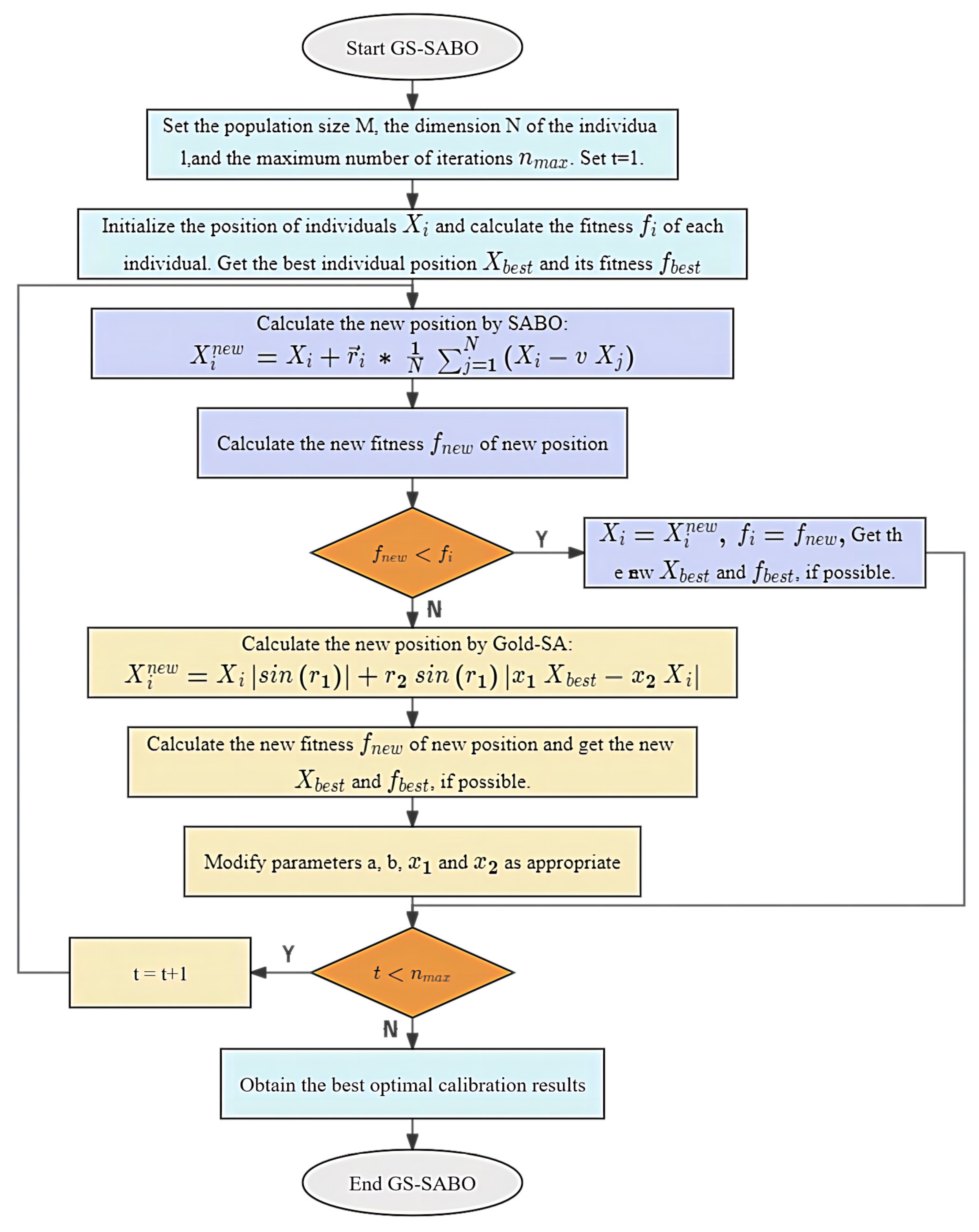
Since SABO does not utilize the global optimum at each iteration but updates the current individual using the positions of all individuals, it is easy to fall into a local optimum solution when the initialized individuals are poorly positioned, which we also verified by algorithmic replication. In order to solve this drawback, we introduce Gold-SA fused with SABO as a novel algorithm called GS-SABO: if the individual adaptation value under the current iteration does not change, the individual position is updated using Gold-SA. This will not increase the computation of the fitness value too much, but also helps the SABO algorithm to jump out the local optimal solution by using the advantage of Gold-SA in the global optimization search. The flowchart of GS-SABO is shown in Figure 5.

4.3.4. All-Pass Filter Parameter Optimization Steps

For an Nth-order all-pass filter, it has N zeros, and to ensure the stability of the filter, these zeros must lie outside the unit circle. These zeros may be on the real axis or not on the real axis. If they are not on the real axis, it requires two dimensions of a population individual to represent one zero. However, when there is a complex zero, there is always a conjugate zero symmetric about the real axis. Therefore, using two dimensions of a particle can represent a pair of complex zeros. So, for N zeros, an N-dimensional vector is needed for representation. If N is even, the odd dimensions represent the real parts of the zeros, and the even dimensions represent the imaginary parts of the zeros. If N is odd, then the first N− 1 dimensions represent complex zeros, and the last dimension represents a real zero.

The algorithm steps are as follows:

Step 1: Calculate residual phase by using Equation (8).

Step 2: Set the population size M, the dimension N of the individual in the population (the order of the filter), the allowable error e, and the maximum number of iterations $n_{max}$. If N is even, the number of complex zeros $N_{cc}=N/2$, the number of real zeros $N_r=0$; if N is odd, the number of complex zeros $N_{cc}=(N-1)/2$, the number of real zeros $N_r=1$. Set the order $N_{shift}$ of the delay line in the all-pass filter system. Set the current number of iterations t = 0.

Step 3: Set M × N initial values, and use Equation (15) to calculate the chaotic initial individual position.

Step 4: Construct complex zeros: $z_k=X_i(2k-1)+X_i\left(2k\right)j,(k=1,2,\dots N_{cc};i=1,2,\dots M)$; if N is odd, then there is also a real zero $x_i\left(N\right)$. Calculate the magnitude of each zero, and if the magnitude is less than 1 take its reciprocal as the new zero.

Step 5: Calculate the response function $Q\left(z\right)$ for each individual:

$$Q\left(z\right)=\prod _{i=1}^{N_r}\left(z_i-z^{-1}\right)\prod _{j=1}^{N_{cc}}\left(z_j-z^{-1}\right)\left(z_j^{\ast }-z^{-1}\right)$$

(18)

Calculate the output phase error by Equations (7), (8), (10), and (11).

Step 6: Calculate the inverse population of the initial population and repeat steps 4–5 using the inverse population to calculate the error function of each individual in the inverse population. Optimize a new initial population by comparing it with the size of the error function of the individuals in the initial population.

Step 7: Construct a new complex zero matrix (same as step 4). Record the size of the error function for each individual of the new initial population. Set the best individual position as $X_{best}$ and the smallest error as $f_{best}$.

Step 8: Calculate the new position of each individual in the population by using Equations (12) and (13). Calculate and record the new error function value of each individual based on the new position. And also record $X_{best}$ and $f_{best}$.

Step 9: Use Equation (14) to determine whether to update the individual position by step 8. If yes, skip to step 13.

Step 10: Calculate the new position of the current individual by using Equation (16).

Step 11: Similar to step 7, calculate the error and record the new $X_{best}$ and $f_{best}$, if possible.

Step 12: Update the Gold-SA coefficients by referring to the coefficient update method in [16].

Step 13: Compare $f_{best}$ with e. If $f_{best}$ < e, skip to step 15.

Step 14: Let $t=t+1$. If the value of t reaches the maximum number of iterations $n_{max}$, skip to step 14; otherwise, skip to step 8.

Step 15: End the iteration to obtain the optimal calibration results and filter parameter settings.

5. Simulation Experiment

5.1. Filter Optimization Algorithm Performance Comparison

In this section, we focus on comparing the improved GS-SABO algorithm with the traditional PSO algorithm when optimizing the all-pass filter parameters.

The wavenumber range of spectra in the simulation experiment was set to be 1000–4000 cm⁻¹ (maximum wave number: 15,802 cm⁻¹). The spectral phase error function was $\theta \left(\omega \right)=0.5sin\left(4\omega \right)$. The computer hardware configuration used in the simulation was 11th Gen Intel (Santa Clara, CA, USA) (R) Core (TM) i5-11300H CPU with 16 GB of memory. We calculated the size of the output phase error by using these two algorithms.

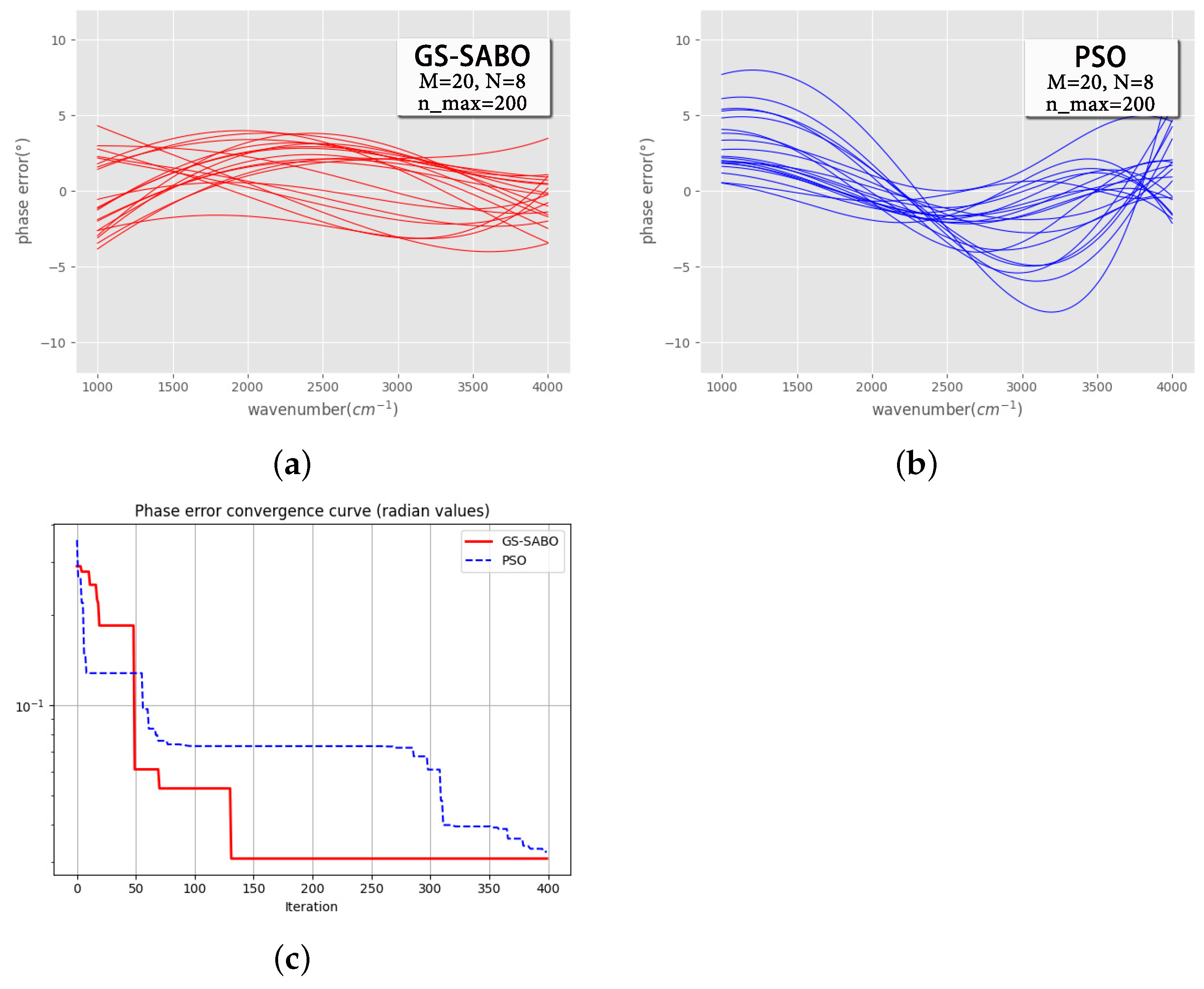
The total number of individuals M = 20, the individual dimension (all-pass filter order) N = 8, and the number of iterations $n_{max}$ = 200. Twenty repetitions of the experiment were performed for both algorithms and the output phase error results obtained are shown in Figure 6a,b. Overall, the correction using the proposed GS-SABO algorithm outperforms the conventional PSO: the average maximum phase error of GS-SABO is ${3.25}^{\circ }$ compared to ${4.43}^{\circ }$ for PSO; and GS-SABO is also better in terms of optimization stability.

We also focus on the convergence of the two algorithms in the all-pass filter optimization problem, and Figure 6c shows the convergence curves of the two algorithms within 400 iterations. Overall, the proposed GS-SABO algorithm has better optimization results, as well as optimization efficiency, with fewer iterations.

5.2. Experiments for PCM-APF Model

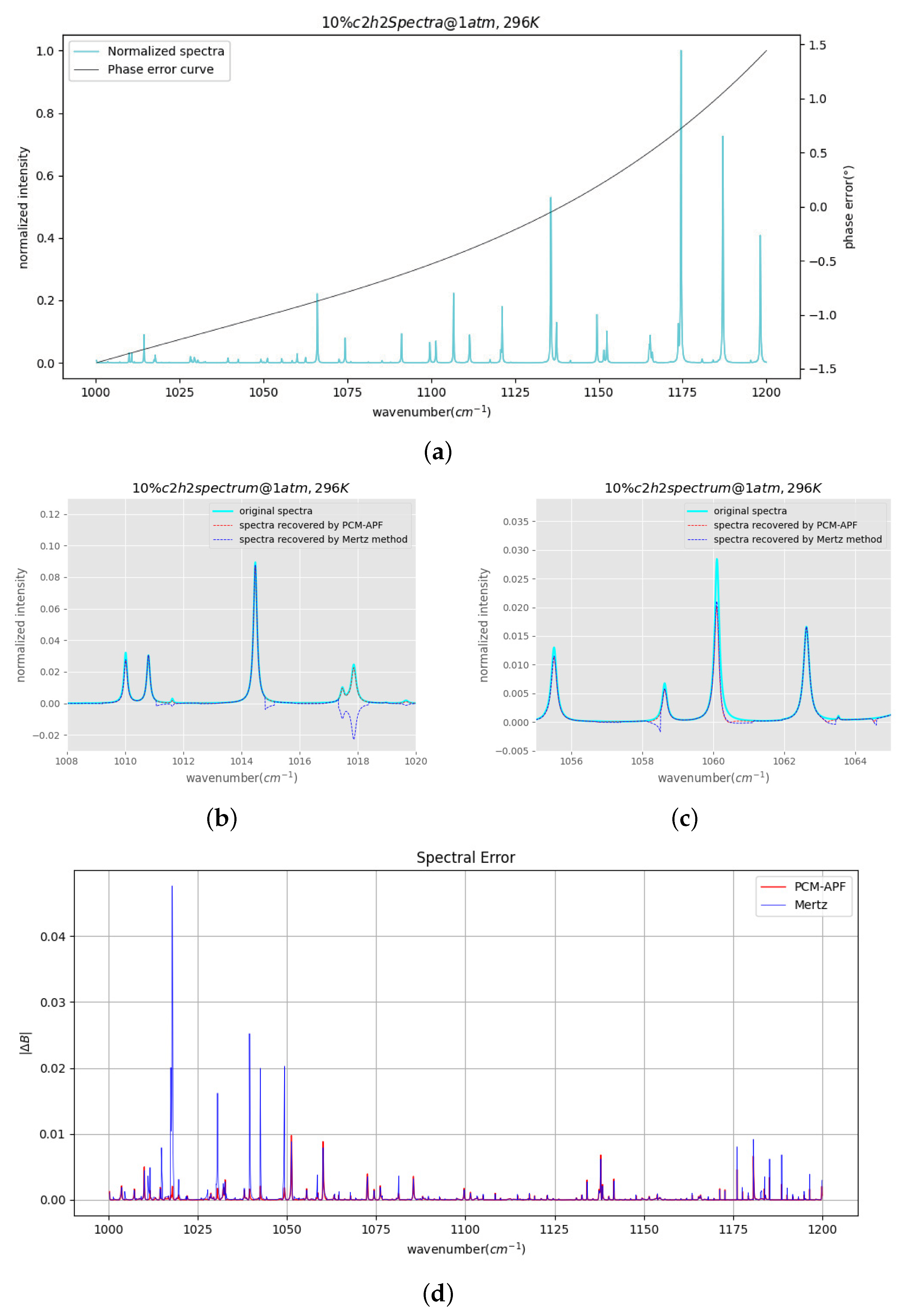
Experiments were conducted using the HITEMP database when comparing the proposed PCM-APF with the Mertz method. HAPI is the Python interface for this database, which allows for various operations such as downloading spectral lines and simulating spectra using encapsulated functions [30]. A simulated emission spectrum was created using air with $10\%$ acetylene gas under standard atmospheric conditions (296 K environmental temperature and one standard atmosphere pressure). The spectral line shape function used was Voigt, and the wavenumber range was 1000–1200 cm⁻¹. Figure 7a displays the normalized spectra after intensity normalization.

Figure 7a also shows the error phase curve (error phase function: $\phi =466.905-765.471\omega +461.631{\omega }^2-122.509{\omega }^3+12.132{\omega }^4$). The proposed PCM-APF model and the traditional Mertz method were employed to correct the nonlinear phase error (with a small number of sample points in the small double-sided interferogram, set to 128). In the PCM-APF model, we set the order of the delay line $N_{shift}=9$ and the order of the all-pass filter N = 8; for the optimization algorithm, the population size M = 20 and the number of iterations $n_{max}$ = 200, using the proposed GS-SABO algorithm.

Figure 7b,c show the spectral curves recovered using the PCM-APF model and the conventional Mertz method in different wavenumber ranges. It can be found that the spectra recovered using the Mertz method have obvious aberrations, especially at the low frequencies of the spectra, which seriously affects the quality of the recovered spectra, which also proves that the Mertz method is indeed deficient in dealing with the problem of nonlinear phase errors. However, the spectra can be well recovered using the proposed PCM-APF model. Figure 7d shows the absolute values of the normalized spectral errors recovered using these two methods. The maximum normalized spectral error of the spectra recovered using the Mertz method is about 0.047, while the value using the PCM-APF model is about 0.008, which is a huge difference, showing the great improvement of the calibration accuracy of the PCM-APF model.

Finally, the parameter settings for the filter calculated by the PCM-APF model are $\{a_0=1, a_1=-1.756691, a_2=1.301406, a_3=-0.871274, a_4=0.626228,$$a_5=-0.525851,$$a_6=-0.133867,$$a_7=0.097102$ and $a_8=-0.001376\}$.

6. Conclusions

In FTS, phase correction techniques typically utilize the well-established Mertz algorithm. However, this method exhibits limited effectiveness in correcting nonlinear phase errors. The all-pass filter technique based on the principles of IIR filtering demonstrates superior performance in terms of both correction accuracy and handling nonlinear phase errors, as convincingly demonstrated in [14]. Building upon this foundation, this paper introduces the use of the phase correlation method, commonly employed in signal delay estimation and image registration, to calculate the linear component of phase errors. The residual phase errors are then corrected using the all-pass filters. Additionally, the improved GS-SABO algorithm employed in the optimization of the filter parameters exhibits favorable properties, particularly rapid convergence.

Overall, through the theoretical analysis and simulation validation presented in this paper, it is evident that our proposed PCM-APF model for phase correction in FTS is a viable and effective approach.

References

- Fomina, P.S.; Proskurnin, M.A.; Mizaikoff, B.; Volkov, D.S. Infrared Spectroscopy in Aqueous Solutions: Capabilities and Challenges. Crit. Rev. Anal. Chem. 2023, 53, 1748–1765. [Google Scholar] [CrossRef] [PubMed]
- Bai, C.; Li, J.; Wang, G.; Lu, C.; Zhang, H.; Zhao, Y.; Zhang, W.; Fu, S. Dual-shearing interferometer for multi-modal hyperspectral imaging. Opt. Lett. 2023, 48, 2214–2217. [Google Scholar] [CrossRef] [PubMed]
- Picqué, N.; Hänsch, T.W. Frequency comb spectroscopy. Nat. Photonics 2019, 13, 146–157. [Google Scholar] [CrossRef]
- Ventura, G.D.; Marcelli, A.; Bellatreccia, F. SR-FTIR Microscopy and FTIR Imaging in the Earth Sciences. Rev. Mineral. Geochem. 2014, 78, 447–479. [Google Scholar] [CrossRef]
- Hashimoto, K.; Nakamura, T.; Kageyama, T.; Badarla, V.R.; Shimada, H.; Horisaki, R.; Ideguchi, T. Upconversion time-stretch infrared spectroscopy. Light Sci. Appl. 2023, 12, 465–474. [Google Scholar] [CrossRef] [PubMed]
- David, A.; Ifarraguerri, A. Computation of a spectrum from a single-beam Fourier-transform infrared interferogram. Appl. Opt. 2002, 41, 1181–1189. [Google Scholar] [CrossRef] [PubMed]
- Forman, M.L.; Steel, W.H.; Vanasse, G.A. Correction of asymmetric interferograms obtained in Fourier spectroscopy. J. Opt. Soc. Am. 1966, 56, 59–63. [Google Scholar] [CrossRef]
- Mertz, L. Correction of phase errors in interferograms. Appl. Opt. 1963, 2, 1332. [Google Scholar] [CrossRef]
- Griffiths, P.R.; Haseth, J.A.D. Fourier Transform Infrared Spectroscopy, 2nd ed.; John Wiley & Sons: New York, NY, USA, 2007; pp. 30–41. [Google Scholar]
- Saptari, V. Fourier Transform Spectroscopy Instrumentation Engineering; SPIE Optical Engineering Press: Bellingham, WA, USA, 2003; pp. 32–34. [Google Scholar]
- Wang, C.L.; Li, Y.S.; Liu, X.B.; Hu, B.L.; Liu, C.F. Detection and Correction of Linear Phase Error for Fourier Transform Spectrometer Using Phase Correction Method. Adv. Mater. Res. 2011, 225–226, 293–296. [Google Scholar] [CrossRef]
- Furstenberg, R.; White, J.O. Phase Correction of Interferograms Using Digital All-Pass Filters. Appl. Spectrosc. 2005, 59, 316–321. [Google Scholar] [CrossRef]
- Wu, X.; Liu, Z.; Li, H. A new model for the phase correction of interferograms. Anal. Methods 2015, 7, 2399–2405. [Google Scholar] [CrossRef]
- Furstenberg, R.; White, J.O. Error-free phase correction of interferograms using digital all-pass filters. Vib. Spectrosc. 2006, 42, 226–230. [Google Scholar] [CrossRef]
- Trojovský, P.; Dehghani, M. Subtraction-Average-Based Optimizer: A New Swarm-Inspired Metaheuristic Algorithm for Solving Optimization Problems. Biomimetics 2023, 11, 149. [Google Scholar] [CrossRef]
- Tanyildizi, E.; Demir, G. Golden Sine Algorithm: A Novel Math-Inspired Algorithm. Adv. Electr. Comput. Eng. 2017, 17, 71–78. [Google Scholar] [CrossRef]
- Liu, Y.; Zhao, Y.C.; Geng, X.R.; Tang, H.R.; Ding, C.B. Analysis of the Phase Error Non-Linearity of FTS and Discussion about Mertz Method. Spectrosc. Spectr. Anal. 2009, 29, 1809–1812. [Google Scholar]
- Huke, P.; Debus, M.; Reiners, A. Phase-correction algorithm for Fourier transform spectroscopy of a laser frequency comb. J. Opt. Soc. Am. B 2019, 36, 1260–1266. [Google Scholar] [CrossRef]
- Fulton, T.; Naylor, D. Fourier Transform Spectroscopy and Hyperspectral Imaging and Sounding of the Environment. In Proceedings of the Fourier Transform Spectroscopy and Hyperspectral Imaging and Sounding of the Environment, Lake Arrowhead, CA, USA, 1–4 March 2015. [Google Scholar]
- Zhang, P.; Zhang, Z. Rapidly changing phase error correction of Fourier transform spectrometer. Chin. J. Lasers 2012, 39, 115002. [Google Scholar]
- Zhang, X.D. Modern Signal Processing; De Gruyter: Berlin, Germany; Boston, MA, USA, 2023; pp. 300–328. [Google Scholar]
- Knapp, C.; Carter, G. The generalized correlation method for estimation of time delay. IEEE Trans. Acoust. Speech Signal Process. 1976, 24, 320–327. [Google Scholar] [CrossRef]
- Nagashima, S.; Aoki, T. A Subpixel Image Matching Technique Using Phase-Only Correlation. In Proceedings of the 2006 International Symposium on Intelligent Signal Processing and Communications, Yonago, Japan, 12–15 December 2006. [Google Scholar] [CrossRef]
- Zhang, Q.Q.; Zhang, L.H. An improved delay algorithm based on generalized cross correlation. In Proceedings of the 2017 IEEE 3rd Information Technology and Mechatronics Engineering Conference (ITOEC), Chongqing, China, 3–5 October 2017. [Google Scholar] [CrossRef]
- Shami, T.M.; El-Saleh, A.A.; Alswaitti, M.; Al-Tashi, Q.; Summakieh, M.A.; Mirjalili, S. Particle Swarm Optimization: A Comprehensive Survey. IEEE Access 2022, 10, 10031–10061. [Google Scholar] [CrossRef]
- Wang, Y.; Dang, C. An Evolutionary Algorithm for Global Optimization Based on Level-Set Evolution and Latin Squares. IEEE Trans. Evol. Comput. 2007, 11, 579–595. [Google Scholar] [CrossRef]
- Rani, G.S.; Jayan, S.; Alatas, B. Analysis of Chaotic Maps for Global Optimization and a Hybrid Chaotic Pattern Search Algorithm for Optimizing the Reliability of a Bank. IEEE Access 2023, 11, 24497–24510. [Google Scholar] [CrossRef]
- Yu, Y.; Gao, S.; Cheng, S.; Wang, Y.; Song, S.; Yuan, F. CBSO: A memetic brain storm optimization with chaotic local search. Memetic Comput. 2018, 10, 353–367. [Google Scholar] [CrossRef]
- Tizhoosh, H.R. Opposition-Based Learning: A New Scheme for Machine Intelligence. In Proceedings of the International Conference on Computational Intelligence for Modelling, Control and Automation and International Conference on Intelligent Agents, Web Technologies and Internet Commerce (CIMCA-IAWTIC’06), Sydney, NSW, Australia, 29 November–1 December 2006. [Google Scholar] [CrossRef]
- Kochanov, R.V.; Gordon, I.E.; Rothman, L.S.; Wcisło, P.; Hill, C.; Wilzewski, J.S. HITRAN Application Programming Interface (HAPI): A comprehensive approach to working with spectroscopic data. J. Quant. Spectrosc. Radiat. Transf. 2016, 177, 15–30. [Google Scholar] [CrossRef]
Figure 1.
An imaging FTS system based on a Michelson interferometer.
Figure 2.
A schematic representation of the selection of two signals in PCM-APF model.
Figure 3.
(a) ZPD offset calculation process in proposed PCM-APF model. (b) The line shape changes in Hilbert difference method and peak detection.