Evaluation of the Urban Weather Generator on the City of Toulouse (France)

Abstract

This article addresses the simulation of urban air temperatures with a focus on evaluating the Urban Weather Generator (UWG) model over Toulouse, France. As urban temperatures, influenced by factors like urbanization, anthropogenic heat release, and complex urban geometry, exhibit an urban heat island (UHI) effect, understanding and mitigating UHI become crucial. With increasing global warming and urban populations, aiding urban planners necessitates accurate simulations requiring data at the canyon level. The paper evaluates UWG’s performance in simulating air temperatures under realistic conditions, emphasizing an operational context and a non-specialist user’s perspective. The evaluation includes selecting the most suitable meteorological station, assessing the impact of the rural station choice, and conducting a sensitivity analysis of input parameters. The validation demonstrates good agreement, with a mean bias error (MBE) of $0.02$ °C and a root mean square error (RMSE) of $1.73$ °C. However, we highlight the fact that UWG performs better in a densely urbanized area, and exhibits limitations in sensitivity to urban surface parameter variations, particularly in less urbanized areas.

1. Introduction

In the context of global environmental changes, the urban heat island (UHI) effect becomes increasingly important with potentially dramatic impacts on human health, biodiversity, air quality, Ref. [1] and other important considerations. City dwellers try to counterbalance the UHI effect with air conditioning, and the energy consumption is then also affected by negative feedback impacts (anthropogenic heat).

Furthermore, energy consumption for space cooling has more than tripled since 1990 [2], with over two billion air conditioners installed worldwide [3]. It is estimated that up to one-quarter to half of the energy used in hot and humid climates is for air conditioning [4]. Therefore, it is of prime importance to understand what causes this phenomenon to occur in the urban landscape to help city planners adapt to new areas able to limit UHI.

With the rapid growth of urban sprawl observed for decades, it becomes increasingly crucial to develop tools to understand and monitor this phenomenon. The UHI effect occurs when cities experience higher air temperatures than their rural surroundings.

Thus, to investigate the impact of urban characteristics on UHI, it is necessary to spatialize air temperature information. However, measuring urban air temperatures is a challenging issue since it is influenced in general by a variety of factors, both natural and anthropic (solar radiation, precipitation, atmospheric movements, human activities, etc.). Urban air temperatures strongly depend on the environment (building, vegetation, traffic, water body, etc.) and the scale at which it is studied from a building to a city level. It is also important to highlight that, faced with the difficulty of extracting precise air temperature measurements, perceptual research has been performed to derive qualitative criteria able to interpret the inconveniences caused by UHI (see [5] for a list of indexes and associated techniques to estimate them). As a consequence, many studies have been developed either to (i) simulate urban temperatures with physical models (see [6] for a recent review); (ii) monitor them with the implementation of local networks ([7,8] or based on crowdsourcing [9]), or (iii) make statistical models that mix local information (land cover, urban morphology) with local measurements to generate maps of UHI [10,11,12]. The reader can find in [13,14,15,16] recent reviews on UHI prediction approaches.

In an application context, and inspired by the description in various review papers, simulation approaches can be classified into three main categories [17]:

• Building-scale models: like EUReCA [18] (relies on energy balance applied to the building volume)
• Micro-scale models: for example, Solene microclimate [19] and Laser-F [20,21] (both based on a modeling of the urban surface geometry at a metric resolution, the Solene microclimate is coupled with an urban airflow model)
• City-scale models (of the order of $100\mathrm{m}$ resolution): among others, we can mention [22,23] (takes into account many physical processes, with an efficient parameterization approach allowing fast numerical simulations over large areas), Solweig [24] (essentially based on radiative exchanges modeling), CitySim [25,26] (based on radiative exchanges and building thermal dynamics modeling), and Envi-met [27] (originally based on airflow modeling, it is the most often used model for microclimate studies. One of its limitations is the calculation of radiation fluxes due to the geometric representation of the urban fabric in an orthogonal grid).

The various microclimatic models differ in the phenomena and scales addressed, ranging from canyon to city level. In some cases, simulations can be very expensive in terms of computer resources and time. Moreover, the data needed for the simulations (physical properties of materials, radiative forcing, etc.) are not always available. Among existing models, Urban Weather Generator (UWG) [28] is an appealing compromise since it is open source, easy to operate, and applicable at a city scale. To our knowledge, this model has been evaluated on nine cities: Toulouse (France) and Basel (Switzerland) [29], Singapore [30], Boston (USA) [31], Rome (Italy) and Barcelona (Spain) [32], Mendoza (Argentina) and Campinas (Brazil) [33], and Abu Dhabi (United Arab Emirates) [34], with slightly different versions since UWG is still under development and continuously updated [35]. The main conclusions made in these papers are (i) that UWG performances are satisfactory with an RMSE of about 1 °C and (ii) that UWG overestimates urban air temperatures during daytime in winter and underestimates nighttime air temperatures in summer.

In this paper, we utilize air temperature predictions to calculate the urban heat island (UHI). To mitigate the extensive deployment of local networks, leveraging simulation models is particularly attractive for estimating air temperatures across various cities and configurations. However, due to the intricacies of the urban environment and the multitude of interactions within it, simulating air temperatures presents a complex challenge with no singular solution; instead, a range of techniques is available. While a prior evaluation was conducted for the city of Toulouse [29], it primarily focused on the experimental periods (BUBBLE and CAPITOUL) and did not specifically address the evaluation of days characterized by a high urban heat island effect—a focus that our paper aims to address. In addition, remote sensing data are used to extract the necessary surface parameters required by UWG. The analysis is conducted on the most urbanized areas in the city of Toulouse (namely Carmes).

The paper is organized as follows: In Section 2, we present the city of Toulouse, its local weather stations network, the UWG model, and finally our evaluation approach of UWG. In Section 3, we analyze the impact of the choice of the rural station on air temperature simulation, present the sensitivity analysis, and study the performances of UWG using residual analysis. We end up with a discussion of our results in light of other studies of UWG before providing some conclusions and perspectives.

2. Materials and Methods

In this section, we first introduce the city of Toulouse and its meteorological network, then the UWG model, and finally the evaluation approach applied in this study.

2.1. Study Site and Associated Data

In this subsection, we describe the study area and the different sources of meteorological data, Metropolitan weather stations as well as Meteo-France stations.

Before describing the site, let us note that validations are based on comparisons between predicted values of temperatures $\widehat{T}$ and measured ones T in validation stations using the Root Mean Square Error:

$$\begin{array}{cc}\hfill RMSE(\widehat{T},T)& =\sqrt{\frac{1}{\mathrm{Card}(t_{max}-t_{min})}\sum _{t=t_{min}}^{t_{max}}{\left(T\left(t\right)-\widehat{T}\left(t\right)\right)}^2}\hfill \end{array}$$

(1)

and the Mean Biased Error:

$$\begin{array}{cc}\hfill MBE(\widehat{T},T)& =\frac{1}{\mathrm{Card}(t_{max}-t_{min})}\sum _{t=t_{min}}^{t_{max}}(T\left(t\right)-\widehat{T}\left(t\right))\hfill \end{array}$$

(2)

with $\mathrm{Card}(t_{max}-t_{min})$ the number of discrete points between $t_{min}$ and $t_{max}$.

2.1.1. City of Toulouse, France

Toulouse is located in southwest France, on the Garonne plain between the Pyrenees and the Massif Central mountains. It is halfway between the Atlantic Ocean and the Mediterranean Sea generating relatively mild winters and warm, sunny summers. It covers $118.3$ km${}^2$. Toulouse is the fourth-largest city in France with a population approaching half a million. With Rennes [36] and Dijon [37,38], Toulouse [39] has one of the most advanced urban meteorological networks in France, enabling acquiring a set of local-scale air temperature data. The Toulouse meteorological network has been deployed since 2017 and new stations are continuously added to enrich the network and enable long-term surveys. The data are freely available (See https://data.toulouse-metropole.fr/ (accessed on 2 December 2023)) [40]. Our choice of the city of Toulouse has been motivated by, among other reasons, its hot summers and favourable meteorological conditions for UHI, as can be seen in

Table 1. Average and Extreme values of some climate variables at Toulouse-Balgnac between 1991 and 2020—Code: 31069001, alt: 151 m, lat: 43°37${}^{\prime }$15${}^{″}$ N, long: 1°22${}^{\prime }$43${}^{″}$ E [41].

	Month	Jan	Feb	Mar	Apr	May	Jun	Jul	Aug	Sep	Oct	Nov	Dec
Climate Var
Mean Temp. (Mean in °C)		6.3	7.1	10.3	12.7	16.4	20.3	22.6	22.8	19.3	15.3	9.9	7
Min Temp. (Mean in °C)		2.9	3.1	5.5	7.9	11.4	15	17	17.1	13.9	10.9	6.3	3.6
Max Temp. (Mean in °C)		9.7	11.2	15	17.6	21.4	25.7	28.2	28.5	24.8	19.7	13.5	10.4
Min Temp. (Extreme in °C)		−18.6	−19.2	−8.4	−3	−0.8	4	7.6	5.5	1.9	−3	−7.5	−12
Max Temp. (Extreme in °C)		21.2	24.1	27.1	30	33.4	40.2	40.2	42.4	35.3	33	24.3	21.1
Precipitation (Mean in mm)		52.5	37.2	45.3	65.2	73.6	64.2	40.1	44.6	45.7	54.3	55	49.3
Wind Speed (Mean over 10 min in ms/s)		3.7	4	4.3	4.3	4.1	3.8	3.7	3.5	3.5	3.7	3.6	3.6

.

2.1.2. Toulouse Metropolitan Weather Station Network

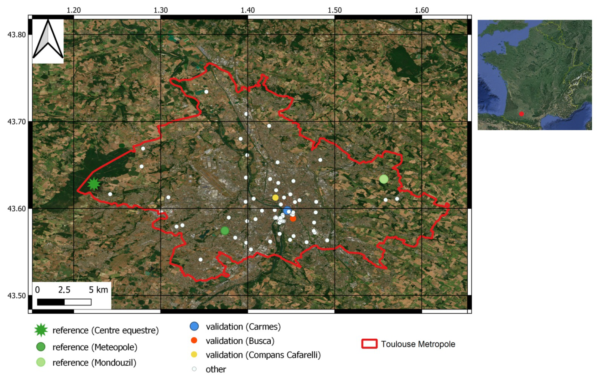
A network of 77 weather stations has been set up in recent years in the Toulouse metropolis to study, among other things, the urban heat island phenomenon. Stations are located in Toulouse and its surroundings and aim at covering the large diversity of land cover. To carry out the implementation of this network, the selection of station sites has been based on a cartographic and field approach [39]. It is important to outline that all measurements have been acquired under a sound protocol to prevent bias between stations. The station network was co-constructed as part of a doctoral research in collaboration with Meteo-France, the French national meteorological institute [42]. To prevent bias in the analysis of air temperatures, each station must be representative of its environment, without being under the direct influence of an isolated element from it (water, vegetation, building, etc.). To ensure representative coverage, it is possible to rely on Local Climate Zones (LCZ) [43] to characterize correctly the land occupation and thus choose appropriately the location of each station [39]. In Figure 1, the localization of the entire network is depicted, on which we highlighted specific stations used in this paper.

2.1.3. Meteo-France Data

Complementary to local station data, Meteo-France, the French meteorological agency, provided us with half-hourly air temperature data, radiative fluxes, and soil temperature measurements acquired at the Meteopole station throughout 2020 [44]. Such data are required, after some processing (averaging, calculation of new variables, etc.) as an input of UWG and these measurements allow us to carry out simulations under realistic conditions, which can therefore be compared to real conditions.

2.1.4. Stations Selected for Validation

Now that we have introduced the weather network stations, combining both Meteopole and Meteo-France stations, we elucidate in the following process how we selected the stations for the validation of UWG in this study. Among the available stations in Toulouse’s network, we first selected three of them for validation. They were chosen since they correspond to three different urban configurations to evaluate the performances of UWG in various LCZs. In practice, they correspond to Compans-Cafarelli in LCZ 11 (i.e., dense trees, urban park), Busca in LCZ 3 (i.e., compact low-rise, outskirts), and Carmes in LCZ 2 (i.e., compact midsize, city center). Their locations are visible in Figure 1. Prior to the evaluation, the results obtained over these three stations were compared to identify the station for which UWG is performing the best. For each urban station under consideration, there are 96 data points (24 h over 4 days). The Carmes station yields the most favorable results, exhibiting the lowest RMSE of $1.73$ °C (refer to

Table 2. Performance indicators of the 3 chosen stations between simulated and measured air temperatures.

Station	RMSE (°C)	MBE (°C)	LCZ [43]
Compans-Cafarelli	$2.35$	$-0.51$	11-Dense trees
Busca	$2.1$	$0.37$	3-Compact low-rise
Carmes	$1.73$	$0.02$	2-Compact mid-rise

) compared to other urban stations in the study. Consequently, the Carmes station was chosen to continue the evaluation analysis.

2.2. UWG: Urban Weather Generator Model

2.2.1. General Description

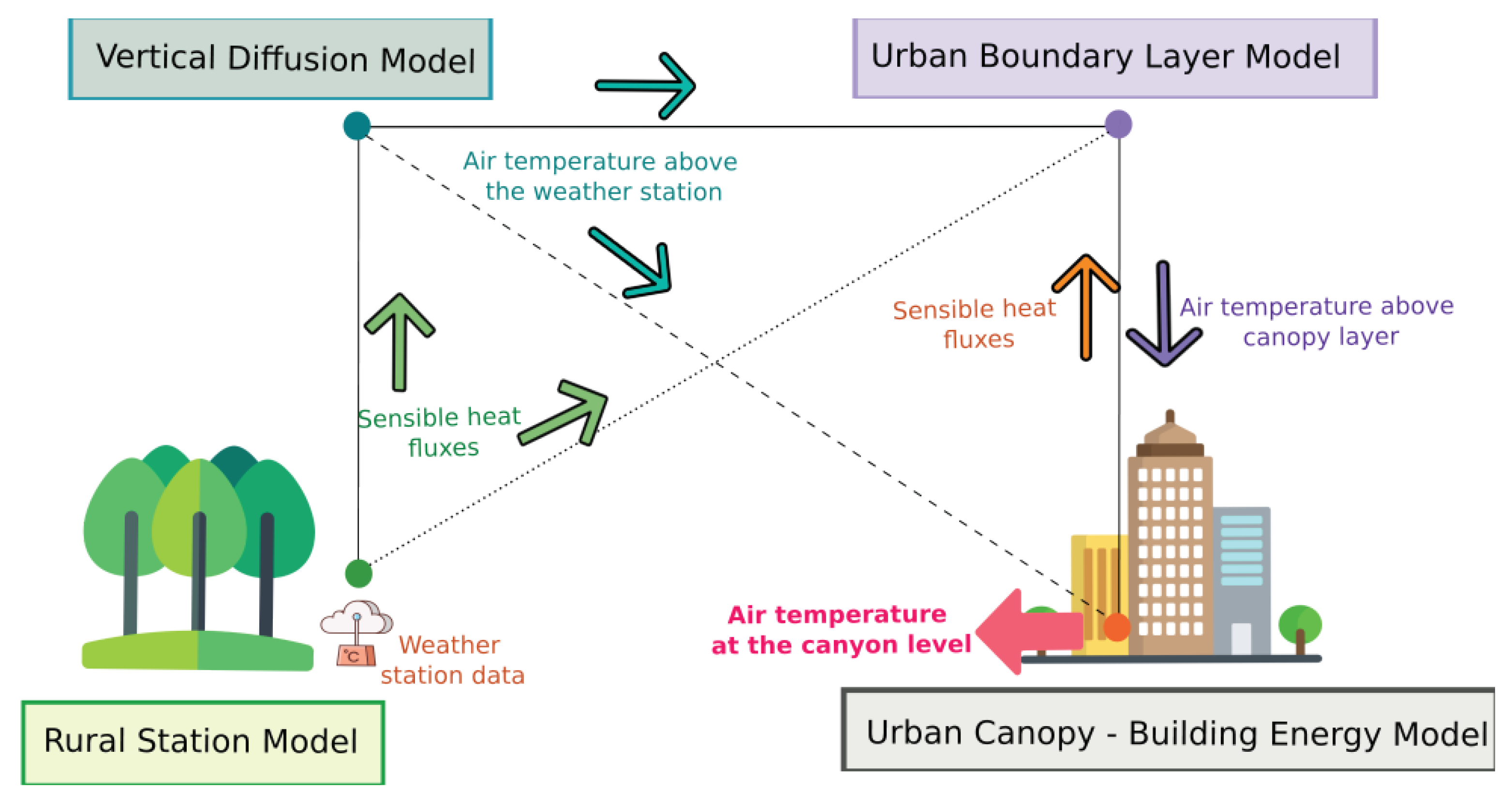
Urban Weather Generator (UWG) is a physics-based simulation model dedicated to urban environments. Given surface parameters associated with relevant meteorological parameters measured at a reference rural weather station, UWG calculates, among other variables, hourly values of air temperature and humidity inside the urban canyon (with a resolution of hundreds of meters). UWG is composed of four coupled modules [45] as we can observe in Figure 2:

• The Rural Station Model (RSM): this corresponds to a rural canopy model that takes hourly values of weather data in a rural reference station (outside urbanized area) and computes sensible heat fluxes that will be used as inputs;
• The Vertical Diffusion Model (VDM): this computes vertical profiles of air temperature above the rural weather station from temperatures, velocities, and sensible heat fluxes calculated issued from the RSM;
• The Urban Boundary Layer (UBL) Model: this module calculates air temperatures above the urban canopy layer from temperatures at different heights provided by the VDM associated with sensible heat fluxes provided by the RSM and the UC-BEM.
• The Urban Canopy and Building Energy Model (UC-BEM): this final module gives air temperature and humidity inside the urban canyon from the RSM module (radiation, precipitation data, air velocity, and humidity) and information above the urban canopy issued from UBL module.

2.2.2. Model Input and Output Data

This part details which data are required to run UWG and how they have been generated in this study. Two families of parameters are required: rural data and urban information. UWG requires two input files: an epw. file in Appendix A and an uwg. file. The first file contains rural station data. The second file contains information on the urban geographic position for which air temperatures will be simulated with UWG.

• Rural data:

We selected three potential reference rural stations: Meteopole in LCZ 5 (i.e., Open midsize), Mondouzil in LCZ 9 (i.e., Sparsely built), and Centre équestre in LCZ 16 (i.e., Bare soil or sand). Mondouzil and Centre équestre belong to rural station criteria as defined in [29]. Despite a more urbanized environment, Meteopole station is also selected as a rural reference as it is located in a rather green area (La Ramée green area park). It is a reference measurement station from Meteo-France and the only rural station over Toulouse where the radiative fluxes and the soil temperatures are acquired. For the other rural stations, the radiative fluxes and soil temperatures used are taken from the Meteopole station. These stations provided us with weather data (air temperature, wind speed, atmospheric pressure, humidity, etc.)

• Data acquired from Meteopole station:

As for meteorological inputs, UWG requires:

• Four radiative fluxes: horizontal infrared radiation, horizontal global radiation, horizontal solar diffuse, and normal solar direct radiation;
• Monthly averages of soil temperatures for three different depths.

We derived these data from Meteo-France measurements at the Meteopole station (see Section 2.1.3) where radiative fluxes and soil temperatures are available.

Table 3. Radiative fluxes according to the CNRM source file and their correspondences in the .epw initialization (file for UWG simulations).

	Source	CNRM File (Source Data)	.epw File (UWG Simulations)
Variable $(\mathbf{W}/{\mathbf{m}}^2)$
Horizontal Infrared Radiation Intensity		Downward Longwave Radiation $\left(LWD\right)$	Horizontal Infrared Radiation Intensity
Horizontal Radiation		Downward Shortwave Radiation $\left(SWD\right)$	Global Horizontal Radiation
Horizontal Solar Diffuse Radiation		Downward Diffuse Shortwave Radiation $(SW\_DIFFUS)$	Diffuse Horizontal Radiation
Normal Solar Direct Radiation		Non-existent in the initial file , calculated with:      $\frac{SWD-SW\_Diffuse}{cos\left(solarzenithangle\right)}$	Direct Normal Radiation

presents the correspondence between the required UWG variables and the source data along with the name of the associated variable in the .epw configuration file required for initializing UWG.

Concerning soil temperature, we choose $1\mathrm{cm}$, $80\mathrm{cm}$, and $220\mathrm{cm}$ depths where an average soil temperature has been computed for each month.

Since we only have one piece of information on radiation issued from Meteopole station given by Meteo-France, we have decided to use the same radiation data for all rural reference stations.

• Urban information:

Parameters describing the surface state of the city are crucial to run UWG. They can be divided into 3 groups, as described below:

• Urban Characteristics. This group concerns local characteristics related to artificialisation and more precisely the density of buildings, their height, and the vertical-to-horizontal ratio. In practice we rely on the BD TOPO 2021, from the French National Institute of Geographic and Forest Information [47], to extract these values. In detail, a Digital Surface Model (DSM) at $1\mathrm{m}$ spatial resolution has been computed from the vector data [47]. From it, the three previously mentioned geomorphological indicators have been computed.
• Vegetation parameters. They represent information related to the vegetation, especially the tree and grass cover ratio. These indicators have been computed at $50\mathrm{cm}$ resolution from BD ORTHO [48]. This has been performed using specific vegetation classification criteria mixed with deep neural networks [49,50,51]. Results have been refined by Computer-Assisted Photo Interpretation (CAPI) [51].
• City information. This optional information is provided by city planners and mainly corresponds to the buildings’ construction era, their nature (residential, commercial, etc.), and the associated LCZ.

The parameters modified (from default values) in this study are detailed in

Table 4. Surface parameters of UWG modified in our study.

Group	Parameter	Description	Carmes Values
Urban Characteristics	bldHeight	Building Height (meters)	$16.71$
Urban Characteristics	bldDensity	Building Density (ratio ranging between 0 and 1	$0.51$
Urban Characteristics	verToHor	Vertical To Horizontal, also called the facade-to-site ratio in some resources on UWG. It is the ratio of the vertical surface area (walls) to the urban plan area. It is defined by: $\sum {\frac{P{h}_{wtd}}{A}}_{site}$ ,where $P=buildingperimeter$, $h_{wtd}=averagebuildingheight$, weighted by footprint, and $A_{site}=totalsitearea$ [28].	$0.9$
Vegetation Parameters	grasscover	Grass Coverage, proportion of grass (ratio ranging between 0 and 1).	0
Vegetation Parameters	treecover	tree Coverage, the proportion of trees in the studied area (ranging between 0 and 1).	$0.06$
City Information	Climate Zone	The American Society of Heating, Refrigerating and Air-Conditioning (ASHRAE) classify International Stations of different countries/zones all around the world into 9 great classes (from 0 to 8) and 19 sub-classes [52].	4A
City Information	bldtype	Building Type from U.S. Department of Energy (DOE) classification. Fifteen commercial building types and one multifamily residential building were determined by consensus between DOE [53].
City Information	bldtera	Building Built Era must be one of the following: “pre80” (pre-1980s), “pst80” (post-1980s), or “new” (new construction).
City Information	bld	Building Array. For each combination building type-building built era, its fraction of the total built stock the building occupies is given.	LargeOffice, Pst80, $0.4$ MidRiseApartment, Pst80, $0.6$

. The surface parameters are first generated at the native spatial resolution of the initial dataset ($50\mathrm{cm}$ or $1\mathrm{m}$) and then aggregated at 200 m using a convolution kernel.

Among optional parameters in UWG, the main ones we modified are all linked to atmospheric conditions, and in particular:

• The Daytime Urban Boundary Layer height in meters , noted h_ubl1;
• The Nighttime Urban Boundary Layer height in meters, noted h_ubl2;
• The Reference Height in meters, noted h_ref. As explained in [45], the reference height is the height at which temperature profiles are uniform (default value = $150\mathrm{m}$). In some resources, reference height is confused with inversion height, which is the height at which the capping inversion occurs (default value = $1000\mathrm{m}$). Capping inversion occurs when the normal temperature (warm air below, cold air above) profile is reversed. This height is the same as the boundary layer height at daytime).

The UWG model outputs simulated values for air temperatures and humidity [29]. Let us now discuss the evaluation methodology.

2.3. UWG Evaluation

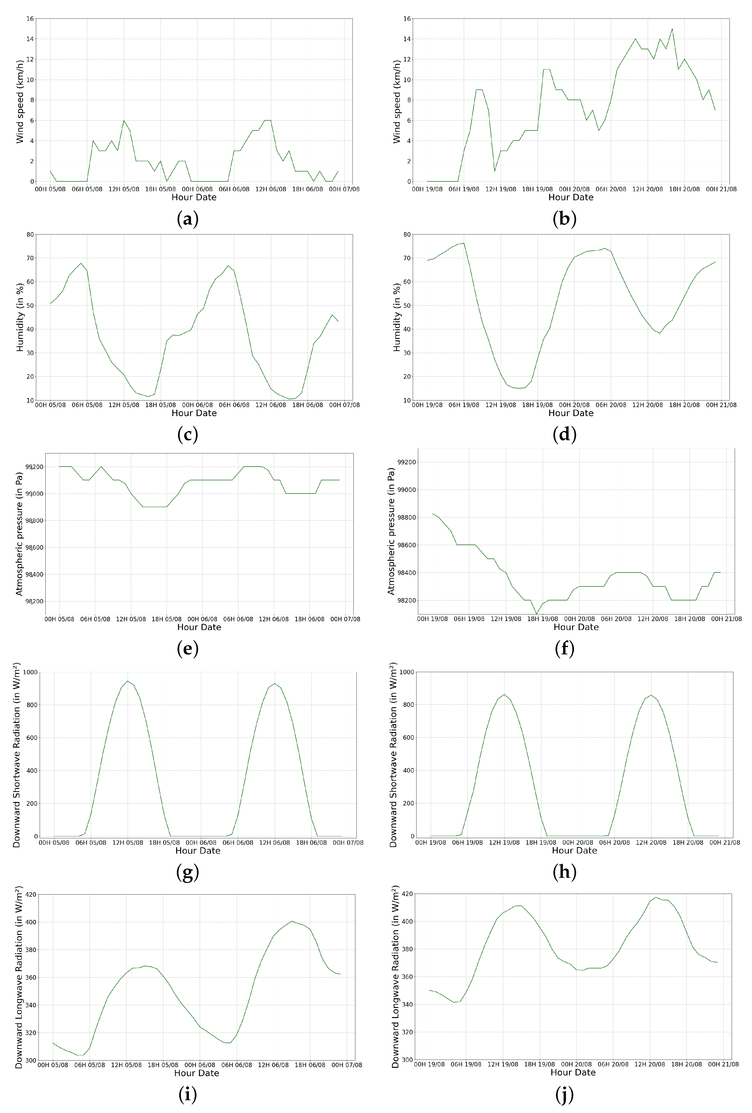
For this study, we select 2 periods of 2 consecutive days where the meteorological conditions are favorable for UHI. They correspond to 5th–6th and 19th–20th of August 2020. On these days, the sky was clear (no decrease in radiation fluxes due to the presence of clouds), atmospheric pressure, humidity, and wind speed were low and therefore air temperatures reached high levels [54] (above 30 °C). The main meteorological variables for these pairs of days are shown in Figure 3.

Formally, from atmospheric, surface parameters and measurements from the rural station, UWG estimates a series of temperatures $\widehat{T}\left(t\right)=UWG({\Theta }_a,{\Theta }_r,{\Theta }_u,t)$ with:

• $UWG$ the UWG model’s function;
• $t\in [t_{min},t_{max}]$ the discrete-time;
• ${\Theta }_a$ the set of $N_a$ input atmospheric parameters: ${\Theta }_a:\left\{{\theta }_{ai}\right\},i\in [1,N_a]$;
• ${\Theta }_r$ the set of $N_r$ input parameters associated with the rural station: ${\Theta }_r=\left\{{\theta }_{ri}\right\},i\in [1,N_r]$;
• ${\Theta }_u$ the set of $N_u$ input internal parameters associated with the urban surface: ${\Theta }_u=\left\{{\theta }_{ui}\right\},i\in [1,N_u]$.

Note that for notation purposes, we also denote $\widehat{T}\left(t\right)=UWG(\Theta ,t)$ with $\Theta$ the set of input parameters: $\Theta =\{{\Theta }_a,{\Theta }_r,{\Theta }_u\}$. As mentioned in Section 2, we evaluate UWG under the view of estimated temperature accuracy in Carmes station. Given that the model depends on a large number of parameters of different natures, to understand into details its behavior, we analyze its accuracy under the view of:

• The impact of the rural station;
• The sensitivity concerning atmospheric and urban parameters;
• The UWG performances that simulate urban temperatures under real conditions.

The methodology associated with these three steps is described in the following three paragraphs.

2.3.1. Impact of the Rural Station

As mentioned in Section 2.2.2, three different rural stations have been chosen: Centre équestre, Meteopole, and Mondouzil. The performance of UWG was evaluated according to the three rural stations by comparing the RMSE and the MBE between predicted values of temperatures $\widehat{T}$ and measured ones T in Carmes station.

2.3.2. UWG Sensitivity Analysis Methodology

To analyze the sensitivity of UWG with respect to its input parameters, the Morris sensitivity analysis method has been exploited [55]. Also known as “the elementary effects” (EE) method, the Morris technique is particularly adapted to models with quantitative inputs/outputs and identifies, in our situation, the input parameters that mainly explain the air temperature outputs. More precisely, it distinguishes parameters with (i) negligible effect on the output; (ii) linear and/or additive effect on the output, and (iii) non-linear effects and/or including interaction with other ones.

In general, a sensitivity analysis method consists of varying all the input parameters in a given range (defined manually based on prior physical knowledge of extreme values of each parameter) and analyzing the sensitivity of the output. As the number of input parameters is large with UWG, computing simulations with all combinations of parameters is in practice impossible from a computational point of view (the problem complexity grows exponentially with the number of parameters). The Morris method proposes an alternative strategy to limit the number of simulations by designing a subset of the entire set of all possible parameter combinations on which to perform the sensitivity analysis.

It relies on screening methods [56] where a set of R trajectories of parameters is computed. A single trajectory ${\Theta }^{\left(k\right)}=[{\Theta }^{\left(k\right)}\left(0\right),{\Theta }^{\left(k\right)}\left(1\right),\cdots {\Theta }^{\left(k\right)}\left(N\right)],k=\{1,\cdots ,R\}$ is a set of $N+1$ parameter variations carefully chosen. Here, N refers to the total number of parameters to analyze. In practice, we focus on atmospheric and urban surface parameters, i.e., $N=N_a+N_u$. As mentioned previously, the influence of the rural station is indeed analyzed in a specific section and the associated parameters ${\Theta }_r$ are not included in the sensitivity analysis.

The idea consists of $(N+1)\times R$ simulations of $UWG$ along all R trajectories and then performs a sensitivity analysis on this subset of parameters instead of on the entire range of possible variations. This leads to a linear complexity with respect to the number of input parameters instead of an exponential one. It has been shown in [57] that this process based on trajectories ensures a reliable representation of input parameter variations and is therefore reliable for a sensitivity analysis. In practice, the set of trajectories is designed as follows:

• Discretization of the parameter space. Each parameter ${\theta }_j\in \{{\Theta }_a,{\Theta }_u\}$ is uniformly split into p levels with a step ${\Delta }_j$ (this latter depends on each parameter’s range of magnitude). We then obtain a grid X of size $N\times p$ containing all possible parameter values;
• Computation of R trajectories. For $i=\{1,\cdots ,R\}$, do the following steps:

  (a)

  Definition of an initial set of parameters ${\Theta }^{\left(i\right)}\left(0\right)$. For the i-th trajectory, a starting set of parameters ${\Theta }^{\left(i\right)}\left(0\right)$ is selected by choosing, for all lines in X, a random value associated with parameter ${\theta }_j,j=\{1,\cdots ,N\}$ among the discretized p-levels;

  (b)

  Generation of a trajectory ${\Theta }^{\left(i\right)}=[{\Theta }^{\left(i\right)}\left(0\right),{\Theta }^{\left(i\right)}\left(1\right),\cdots ,{\Theta }^{\left(i\right)}\left(N\right)]$. From the initial set of parameters ${\Theta }_{\left(i\right)}\left(0\right)$, a sequence of $N+1$ parameter set is designed in a sequential way for $j=\{1,\cdots ,N\}$ as follows:

  • The parameter set ${\Theta }^{\left(i\right)}\left(j\right)$ is derived from ${\Theta }^{\left(i\right)}(j-1)$ by adding to the value of parameter ${\theta }_j$ in ${\Theta }^{\left(i\right)}(j-1)$ a random step $\pm {\Delta }_j$ in a positive or negative direction. Other values of parameters ${\theta }_k,k=\{1,\cdots ,N\},k$ remain unchanged.

After this process, we have a set of R trajectories where each trajectory ${\Theta }^{\left(i\right)}$ corresponds to $N+1$ specific variations of parameters (the difference between two successive sets ${\Theta }^{\left(i\right)}\left(j\right)$ and ${\Theta }^{\left(i\right)}(j+1)$ is only on parameter ${\theta }_{j+1}$. Simulations are then performed on all R trajectories. The Morris method relies on several concepts to analyze the sensitivity of a given parameter ${\theta }_j$. They are described below.

• The mean of the absolute elementary effects:

For each parameter ${\theta }_j$, its effect on the variation of $\widehat{T}$ among all the R trajectories is quantified, for any time step t, by ${\mu }_j\left(t\right)$ computed as:

$$\begin{array}{cc}\hfill & {\mu }_j\left(t\right)=\frac{1}{R}\sum _{i=1}^R\left|d_{i,j}(T,t)\right|with\hfill \\ \hfill & d_{i,j}(T,t)=\frac{UWG({\Theta }^{\left(i\right)}\left(j\right),t)-UWG({\Theta }^{\left(i\right)}(j-1),t)}{{\Delta }_j},\mathrm{t}\mathrm{h}\mathrm{e} \mathrm{e}\mathrm{l}\mathrm{e}\mathrm{m}\mathrm{e}\mathrm{n}\mathrm{t}\mathrm{a}\mathrm{r}\mathrm{y} \mathrm{e}\mathrm{f}\mathrm{f}\mathrm{e}\mathrm{c}\mathrm{t} \mathrm{o}\mathrm{f} \mathrm{p}\mathrm{a}\mathrm{r}\mathrm{a}\mathrm{m}\mathrm{e}\mathrm{t}\mathrm{e}\mathrm{r} {\theta }_j\mathrm{at} \mathrm{the} \mathrm{trajectory}\hfill \end{array}$$

(3)

Roughly , $d_{i,j}$ quantifies the effect on the output of variations of parameters ${\theta }_j$, since only ${\theta }_j$ varies between ${\Theta }^{\left(i\right)}(j+1)$ and ${\Theta }^{\left(i\right)}\left(j\right)$. In practice, to evaluate the relative importance of all variables among them, we calculate the normalized mean of absolute elementary effects ${\mu }_j^{*}$ defined as:

$${\mu }_j^{*}\left(t\right)=\frac{{\mu }_j\left(t\right)}{{\displaystyle \sum _{k\in \Theta }}{\mu }_k\left(t\right)}.$$

(4)

This normalized quantity enables us to evaluate the relative importance of one variable ${\theta }_j$ with respect to all others by providing a value ${\mu }_j^{*}\left(t\right)$ in the interval $[0,1]$ with ${\displaystyle \sum _{k\in \Theta }}{\mu }_k^{*}\left(t\right)=1$.

• The standard deviation ${\sigma }_j$ of the elementary effects:

For each input parameter ${\theta }_j$, the standard deviation of elementary effects is defined as:

$${\sigma }_j\left(t\right)=\sqrt{\frac{1}{R-1}\sum _{i=1}^R{\left(d_{i,j}(T,t)-{\mu }_j\left(t\right)\right)}^2}.$$

(5)

This value accounts either for non-linearities in the influence of ${\theta }_j$ (the higher the value, the more non-linear the influence of the associated parameter) or for interactions between input variables (${\theta }_j$ interacts with at least another variable). On the contrary, a low standard deviation means that the influence of ${\theta }_j$ output is linear on the temperature’s estimations and has no interaction with other inputs.

As a matter of fact, the standard deviation is computed for elementary effects associated with a single input parameter. More precisely, if the studied parameter ${\theta }_j$ varies by a given quantity ${\Delta }_j$, the associated elementary effect for d is the variation of the output divided by ${\Delta }_j$. Computing the standard deviation of the elementary effect for all possible variations of ${\Delta }_j$ is therefore informative. Indeed, if this standard deviation is equal to zero, it indicates that regardless of the variation in ${\Delta }_j$, the elementary effect is homogeneous (in other words, the output varies linearly with respect to ${\theta }_j$). In contrast, if this standard deviation is not equal to zero, it indicates that the output varies either non-linearly with respect to ${\theta }_j$ or that the studied parameter is correlated with another one.

It has been shown in [57] that values of ${\mu }_j$ and ${{\sigma }_j}^2$ computed on the set of trajectories are unbiased estimators of the actual mean and variance of the true distribution of input parameters. This process is then used to analyze the sensitivity of UWG with respect to the set of input parameters. In practice, atmospheric and surface parameters have been set based on plausible (and acceptable for UWG) extreme values. The complete list of input parameters used, their extreme values, and associated discretization steps in the sensitivity analysis process are visible in

Table 5. UWG input parameters’ variation ranges used in the sensitivity analysis. The short name associated with the description of parameters corresponds to the names used in the figures in the experimental part.

Param.	Description (Short Name)	Unit	Family	Min.	Max.	Step ${\mathbf{\Delta }}_{\mathit{j}}$
${\theta }_1$	Building height (bldHeight)	meters (m)	urban surface ${\Theta }_u$	3	70	$7.4$
${\theta }_2$	Building density (bldDensity)	– (ratio)	urban surface ${\Theta }_u$	$0.1$	1	$0.1$
${\theta }_3$	Grass cover (grasscover)	– (ratio)	urban surface ${\Theta }_u$	0	1	$0.11$
${\theta }_4$	Tree cover (treecover)	– (ratio)	urban surface ${\Theta }_u$	0	1	$0.11$
${\theta }_5$	Facade length (facade length)	meters (m)	urban surface ${\Theta }_u$	4	4270	474
${\theta }_6$	Roof albedo (albRoof)	– (ratio)	urban surface ${\Theta }_u$	$0.1$	$0.7$	$0.07$
${\theta }_7$	Road albedo (albRoad)	– (ratio)	urban surface ${\Theta }_u$	$0.1$	$0.7$	$0.07$
${\theta }_8$	Wall albedo (albWall)	– (ratio)	urban surface ${\Theta }_u$	$0.1$	$0.7$	$0.07$
${\theta }_9$	Vegetation albedo (albVeg)	– (ratio)	urban surface ${\Theta }_u$	$0.05$	$0.5$	$0.05$
${\theta }_{10}$	Daytime urban boundary layer (ublday)	meters (m)	atmosphere ${\Theta }_a$	800	2000	$133.34$
${\theta }_{11}$	Nighttime urban boundary layer (ublnight)	meters (m)	atmosphere ${\Theta }_a$	30	100	$7.7$
${\theta }_{12}$	Reference height (href)	meters (m)	atmosphere ${\Theta }_a$	100	200	11

.

2.3.3. Analysis of UWG Performances

Once the impact of the rural station is evaluated as well as the sensitivity analysis, in a third step we evaluate UWG simulations on Carmes station. As already mentioned, this station is indeed the most urbanized area and therefore the most likely to be submitted to UHI. It is also the one where UWG performed the best (see Table 2) which is also consistent with the observation made in [58] where UWG performs better in densely urbanized areas.

In addition to the usual evaluation criteria, we also rely on standardized residuals. A standardized residual $z_k\left(t\right)$, associated with a simulation ${\widehat{T}}_k=UWG({\Theta }^k,t)$ (with ${\Theta }^k$ a given set of parameters), is defined for any time step t by comparison with the measured temperature $T\left(t\right)$ as:

$$\begin{array}{cc}\hfill z_k\left(t\right)& =\frac{{\widehat{e}}_k\left(t\right)}{{\sigma }_k}\mathrm{with}\hfill \\ \hfill {\widehat{e}}_k\left(t\right)& =T\left(t\right)-{\widehat{T}}_k\left(t\right)\mathrm{the}\mathrm{residual}\mathrm{at}\mathrm{time}t\mathrm{and}\hfill \\ \hfill {\sigma }_k& =\sum _{t=t_{min}}^{t_{max}}{\widehat{e}}_k^2\left(t\right).\hfill \end{array}$$

(6)

A small standardized residual means a reliable estimation and it is common to assume that a standardized residual of magnitude higher than 3 (or lower than $-3$) is considered an outlier [59]. This approach is then useful to easily identify outliers.

Let us now turn to the experimental results.

3. Experimental Results

In this section, we analyze UWG under the three points mentioned above: impact of the rural station, sensitivity analysis, and UWG performances.

3.1. Impact of the Rural Station

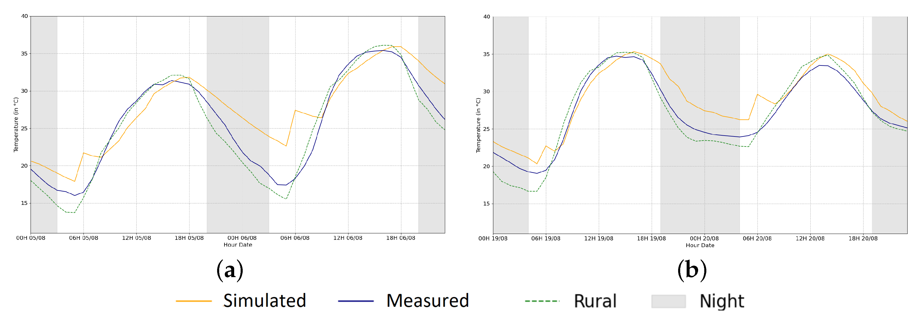
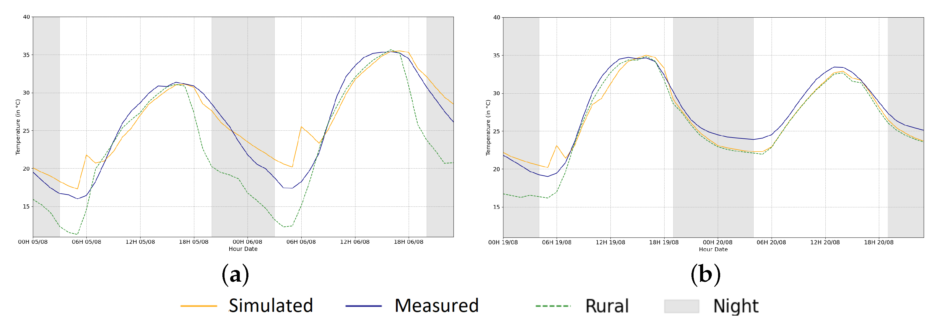
As described in Section 2.2, UWG needs information issued from a rural station (to obtain the climatic context outside the city). These meteorological data include radiative fluxes and soil temperature. As shown in [30], this reference weather station impacts the quality of the estimation and it is then important to select the most adapted one. We then analyze, on the selected two pairs of days, the accuracy of UWG estimations in Carmes station for the three selected rural stations (Meteopole, Mondouzil, and Centre équestre, see Section 2.2.2). In Figure 4, Figure 5 and Figure 6 are depicted, for Meteopole, Mondouzil, and Centre équestre:

• The temperature at the rural station (dashed green);
• The simulated temperature for Carmes with UWG (yellow);
• The measured temperature in Carmes station (blue).

Quantitative values of associated RMSE and MBE are visible in

Table 6. Performance indicators between simulated (based on the 3 rural stations) and measured air temperatures.

Rural Station	RMSE °C	MBE °C
Mondouzil	$3.48$	$-2.24$
Meteopole	$3.39$	$-2.22$
Centre équestre	$1.73$	$0.02$

. As shown in Figure 4, Figure 5 and Figure 6, there is an overall good agreement between the simulated air temperature and the values measured at Carmes station. However, the RMSE and MBE, ranging, respectively, from $1.73$ °C to $3.48$ °C and $-2.24$ °C to $0.02$ °C, show that the estimation accuracy varies according to the rural station. We observe in all cases, an overprediction of the air temperature starting in the middle of the night until early morning followed by a slight underprediction until sunset. In addition, abnormal peaks occur around 4 a.m. (which corresponds to the sunrise UTC hour) and this is regardless of the rural station used for the simulation. In one paper [30], the authors, explain these peaks: they occur during the night–day and day–night transitions as the underlying UBL submodel inside UWG relies on two different sets of equations (before and after the transition). According to [30], these discontinuities are reduced by the thermal inertia of the UBL air and can be attenuated by slightly modifying the shifting times between night and day.

Even if the Meteopole station is located closer to the city in a less rural environment, the simulated air temperature based on this station fits slightly better the measurements of Carmes station based on rural station Meteopole than the one simulated based on Mondouzil station, with an MBE of $-2.22$ °C and $-2.24$ °C and RMSE of $3.39$ °C and $3.48$ °C, respectively, (Table 6).

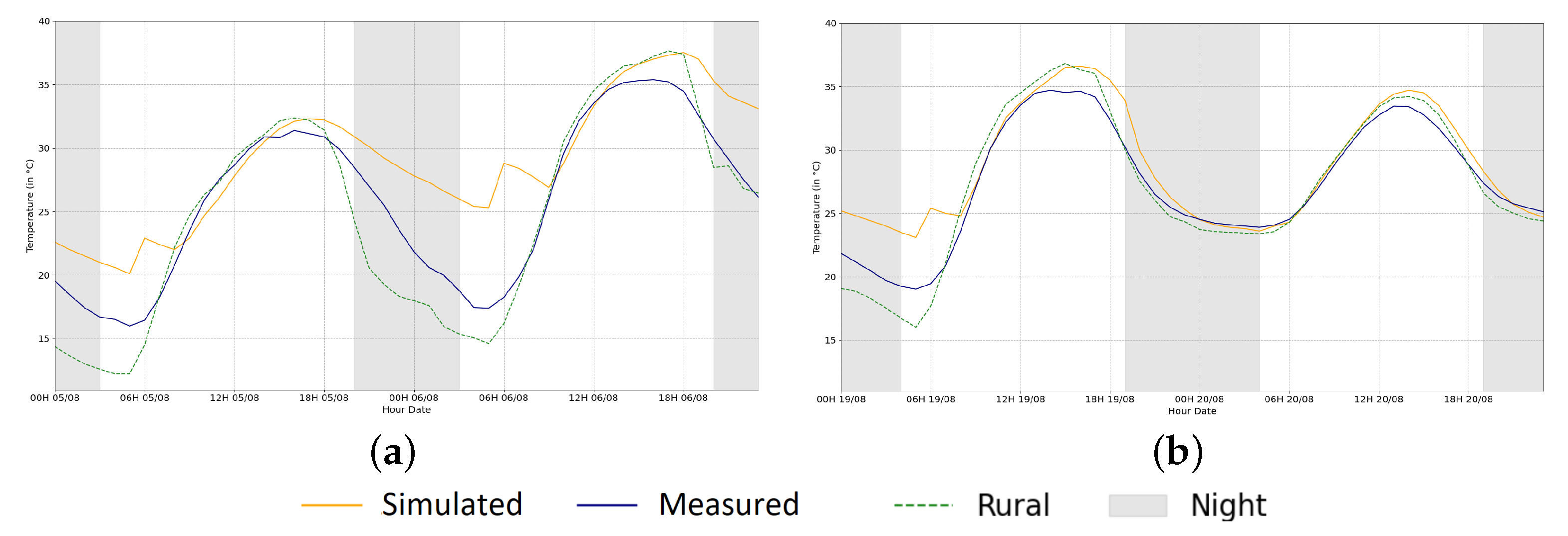
Simulations based on rural data from Centre équestre station stick the best to measured values (Figure 6) with an MBE of $0.02$ °C and an RMSE of $1.73$ °C (Table 6). The absence of anomaly peaks in the simulated air temperatures for Carmes, Meteopole, and Centre équestre rural stations on the 20th of August can be explained by the fact that the night before was the hottest of the studied period (minimum 22 °C). Therefore, there is a low difference between the rural and in-city air temperature values for this specific day (e.g., the meteorological conditions may not been entirely favorable to UHI). Of course, this point would require further investigation.

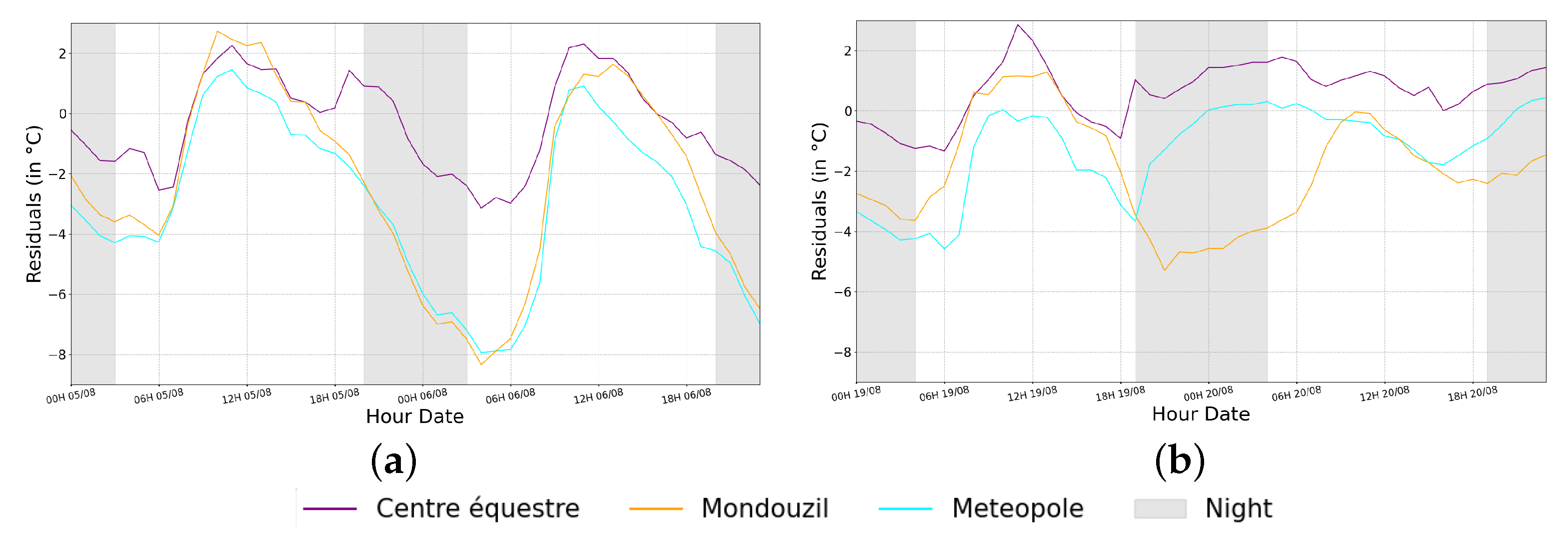
In the following results, the anomalies have been filtered out and linearly interpolated, as also suggested in [58]. With these corrections, it is even more obvious in Figure 7 that the simulated air temperatures at the Carmes station, based on Centre équestre rural station, have the lowest error along the studied period. In addition, these results highlight the importance of the choice of the rural station for UWG to accurately simulate air temperatures.

3.2. Sensitivity Analysis

The sensitivity analysis of a model such as UWG is an essential step given the large number of input parameters used. As introduced in Section 2.3.2, we rely on the Morris technique whose goal is to identify, with a specific selection of input parameters, how a variation of one input influences the temperature by computing the normalized elementary effects (see Equation (4)) and their standard deviation (see Equation (5)).

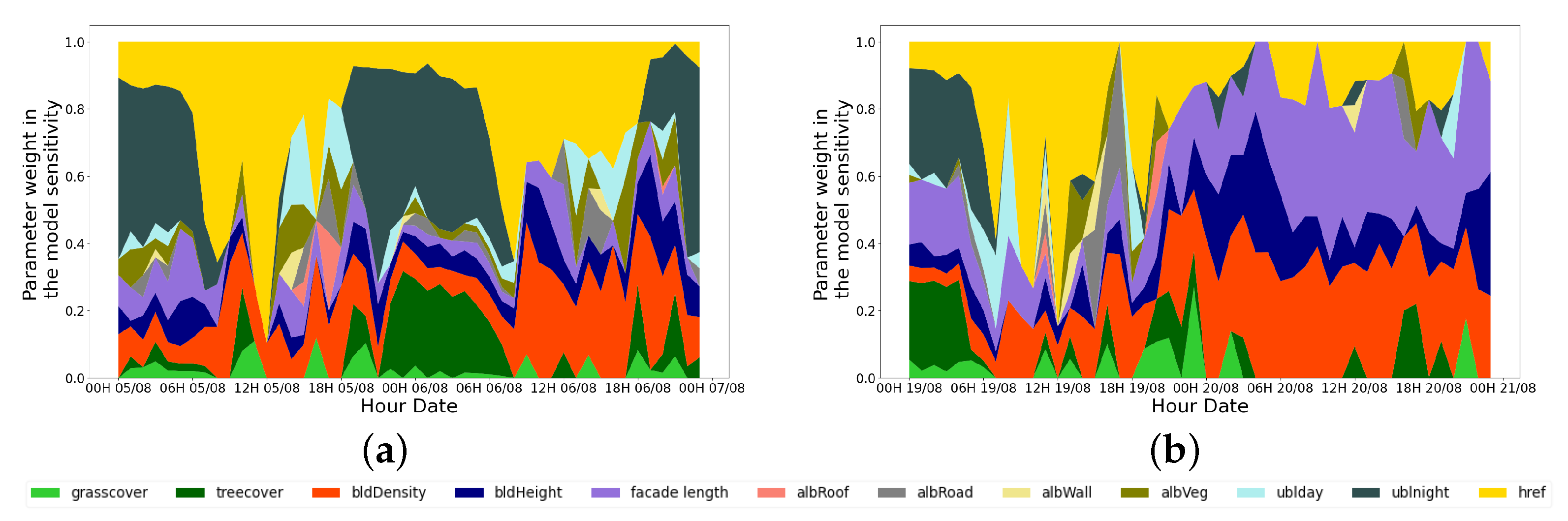
We have depicted in Figure 8a,b the normalized elementary effects of each variable shown in Table 5 along the two chosen pairs of days for the evaluation. The complete description of each input parameter can be seen in Table 5. The objective of this analysis is to order the inputs according to their importance in the model so the quantitative (non-relative) impact of each parameter can not be known. As can be seen in these figures, atmospheric variables (nighttime urban boundary layer height and reference height) seem to have the most impact on the sensitivity of the results. This point will be developed further in Section 4.

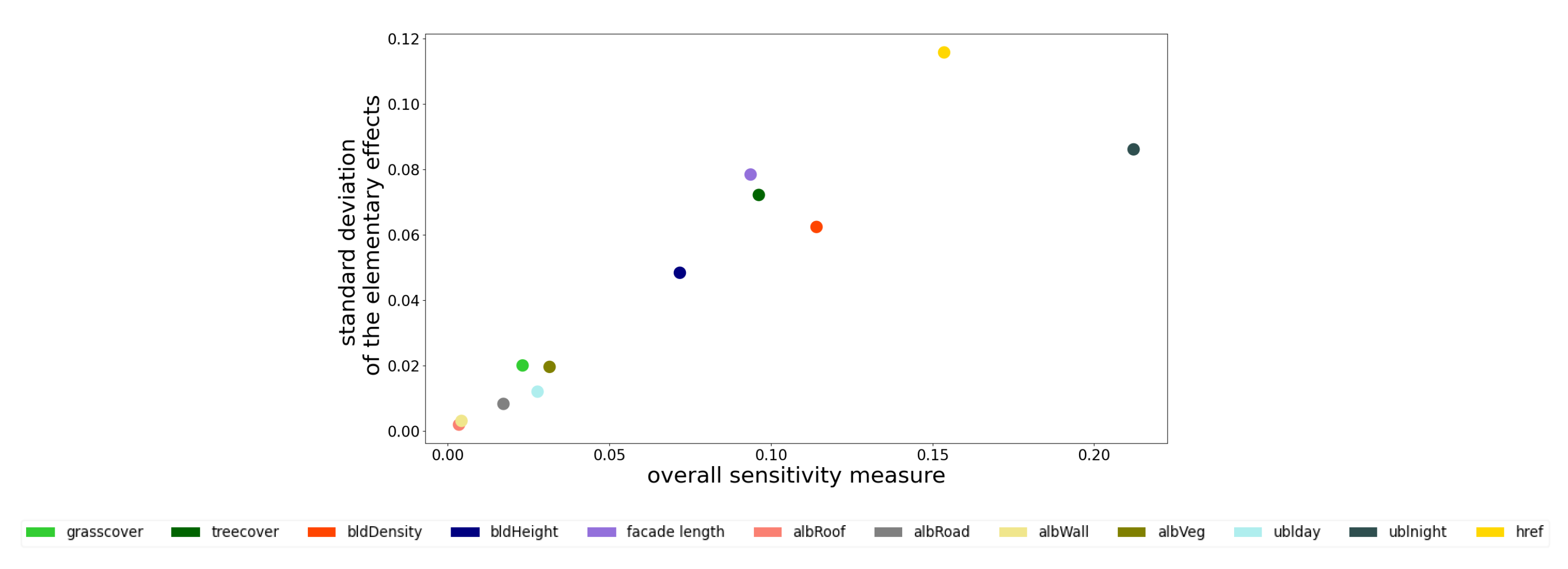
Figure 8a,b shows the impact of each variable on the accuracy of the result. To go more into detail on the interaction of the variables between them, we have plotted in Figure 9, for each variable, the standard deviation of the elementary effect (see Equation (5)) against the elementary effect itself (see Equation (5)). These values have been averaged during all time steps in order to have a global evaluation of the influence of each variable. The interest of such a representation is to highlight three situations:

• Input parameters that have a low influence on UWG’s output temperatures. The corresponding points are close to the origin since their averaged elementary effects as well as their standard deviations are small;
• Input parameters that have a linear influence on UWG’s output temperatures. The corresponding points follow a line: their standard deviations are proportional to their elementary effects;
• Input parameters that have a nonlinear influence on UWG’s output temperatures or that are in interactions together. Associated points are those that differ from the line mentioned above.

As can be seen in Figure 9, all albedo variables, grass cover, and daytime boundary layer have almost no effects on the output (first situation listed above). Tree cover and other surface parameters (building height, facade length, and building density) have a linear influence on the temperature, noting however that building density (from $0.1$ to $0.8$) has a stronger impact on air temperatures of up to $5.6$ °C (second situation listed above, see Figure 10c). Reference height $href$ has also an important linear impact on air temperature. Nighttime urban boundary layer height $ubl\_night$ is in the third situation, i.e., has a non-linear influence or is in interaction with other variables. Since it is the only variable in this situation, it is likely that it has a non-linear influence on UWG’s output air temperature rather than an interaction effect with other inputs.

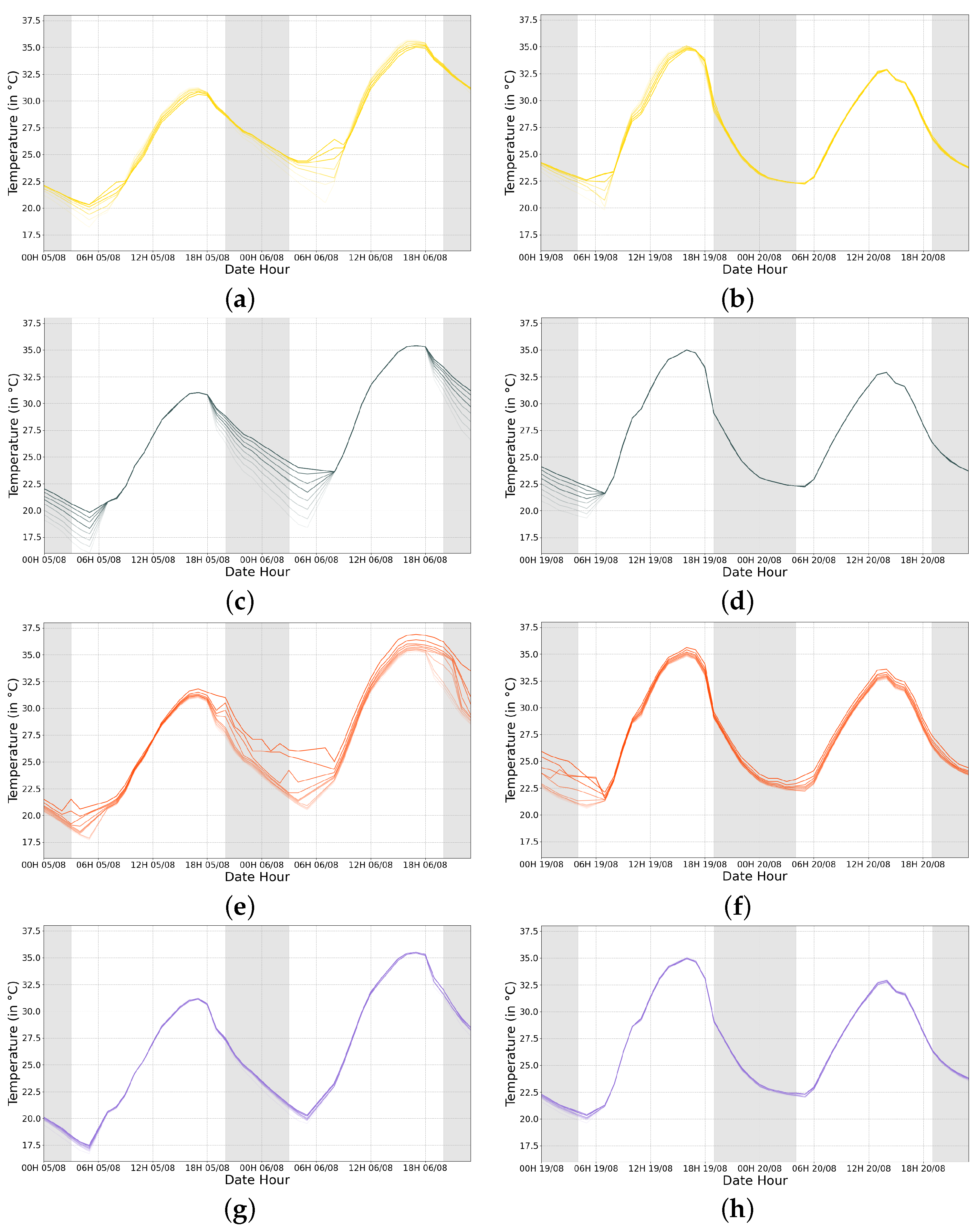
To quantitatively assess the influence of the input parameters, we have plotted the simulated air temperatures at Carmes station for the eight most influential parameters in Figure 10. As can be seen, the atmospheric parameters in Figure 10a–d and the building density in Figure 10e,f show the greatest variability in the simulated air temperatures (up to $0.87$ °C on average). In contrast, surface parameters such as facade length in Figure 10g,h have a small influence on the variability of the output (up to $0.16$ °C on average).

3.3. Analysis of UWG Performances on UHI Days

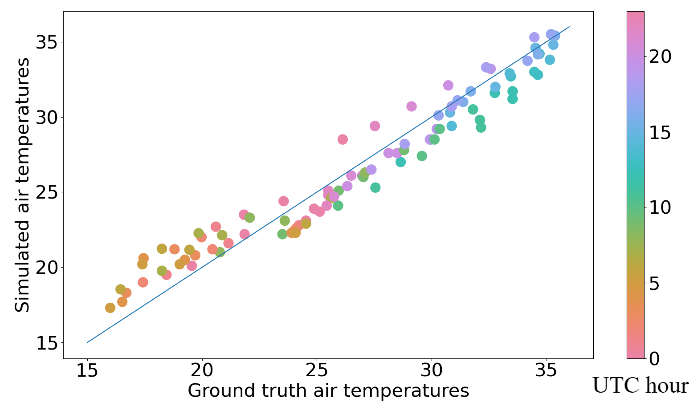
We now analyze UWG performances on simulated air temperatures during the two pairs of days submitted to UHI. To this end, we have depicted in Figure 11 the simulated vs. measured air temperatures at Carmes station. The blue line corresponds to the ideal situation where $\widehat{T}=T$ and enables us to indicate how far/close from the measurements our simulations are. We also represent each point in a different color according to the simulation hour to highlight behaviors correlated to the period of the day. This figure shows that the simulations overestimate air temperatures rather in the middle of the night until early morning (left part of the figure where points correspond to the morning and are up to the blue line) while they underestimate them in the afternoon (right part of the figure where points correspond to the afternoon and are below the blue line).

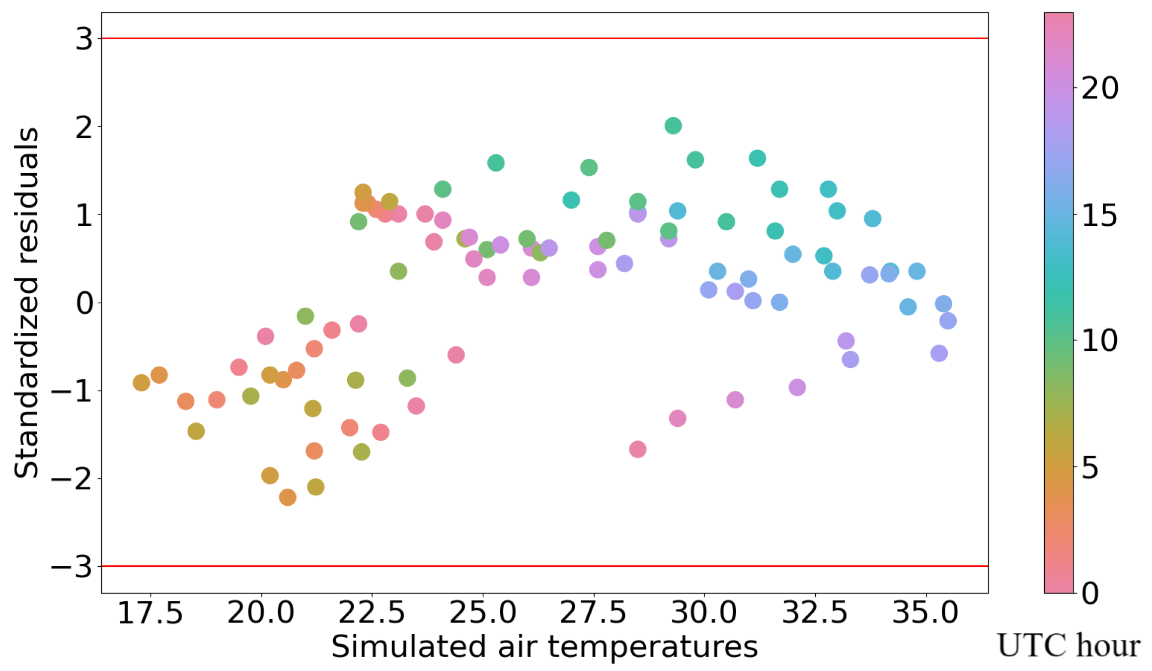
To evaluate the most relevant/irrelevant simulations, the standardized residuals (see Section 2.3.3) are depicted in Figure 12 in the function of simulated air temperatures. A similar color in the function of the hour of the day has been used. As previously mentioned, a value higher than 3 (i.e., 3 times the standard deviation which has been normalized to 1) indicates a too-large error that can be considered as an outlier. It is interesting to note that no outliers have been simulated in this case (which is a good property). However, two groups can be identified on this figure depending on the time of simulation:

• Late night and morning hours (from midnight to 9 a.m.) have negative standardized residuals and low simulated air temperatures. In this situation, air temperatures are overestimated by UWG;
• Afternoon and evening hours (from 10 a.m. to 8 p.m.) have positive standardized residuals and high simulated air temperatures. In this situation, air temperatures are underestimated by UWG during the daytime.

These observations are consistent with Figure 11 but the standardized residual analysis enables guaranteeing that UWG simulates relatively consistent air temperatures without outliers.

4. Discussion

As mentioned in previous sections, UWG enables simulations of urban air temperatures from a set of input parameters associated with atmospheric, urban surface occupations, and rural climatic conditions. In Section 3, we have evaluated the influence of the rural station, the sensitivity of UWG with respect to its main input parameters, and its ability to retrieve reliable air temperatures. All measured data used for comparison purposes are issued from the Carmes weather station, located in a densely built environment in the center of Toulouse, France. As already observed in [58], UWG performs better in densely urbanized areas. Before discussing the results presented in Section 3, it is important to recall that the observations and conclusions made in this study have to be interpreted considering that we only modified a limited number of parameters for the initialization of UWG. A finer tuning of the parameters, for example in the building description files or the code itself, would probably lead to different results. The idea was to use UWG as a basic user, modifying only accessible parameters with available input data such as in operational use.

4.1. Influence of the Rural Station

The analysis of Section 2.3.1 highlights that the choice of the rural station has a significant impact on the simulation results and performance. This differs from [30] who tested UWG (2014 version) under the humid tropical climate of Singapore and concluded that the location of the rural station did not have a major impact on the simulation.

Several reasons may explain these opposite observations. First, from a geographic point of view, the city of Toulouse is characterized by a fairly urbanized center and a more pronounced green belt, whereas Singapore looks more like a continuum of urbanization. In this context, the localization of the rural station is less sensitive in Singapore because of the low urban gradient. Besides, Singapore is surrounded by the sea. Therefore, finding a rural station away from a body of water, as recommended in the rural station selection criteria, seems to be difficult. The second reason may be the different climate of Toulouse and Singapore that are completely different. Singapore has indeed an equatorial climate with two seasons, wet and dry, while the climate of Toulouse is generally characterized by four seasons having relatively mild winters and hot summers where the frequency of UHI is higher (and the difference with the rural station amplified). These points can explain our observation that, in our study, the choice of the rural station is significant, especially on days that are favorable to UHI, unlike observations made in [30].

In practice, the fact that the Meteopole station is still inside the urbanized area of Toulouse, even if located in a green area, may explain its poor ability to provide a proper rural climate context. Even if Mondouzil is located further from Toulouse city center, Figure 1 shows that this station is close to the built-up area. Consequently, its measurements may be influenced by surrounding urbanization. Finally, the Centre équestre station, far away from the city and rather in green areas, appears as the rational choice. A more detailed analysis of the local climatic context would help to better understand these results.

For a generalization of the use of UWG, it would be relevant to deepen this investigation on the impact of the location of the rural station.

4.2. Sensitivity Analysis

From the sensitivity analysis presented in Section 3.2, three main observations can be made:

• First, as shown in Figure 8 concerning elementary effects, forcing atmospheric parameters are the main drivers of the simulation. Parameters ublnight associated with the nighttime urban boundary layer and href associated with reference height (see Table 4) are indeed the most represented (ublnight represents almost $50\%$ of the contribution of all parameters to the sensitivity of UWG at night, versus almost $35\%$ for href during the day) and have an important weight in the simulation. In practice, unlike the other forcing parameters of the rural station, these values are fixed at initialization (the temporal evolution is not provided by the user). Given their influence in the simulation, this is a main limitation of UWG. This has already been observed in [60] who performed an urban boundary layer height empirical estimation (based on Paris data). Such values are difficult to acquire in practice. Meso-NH [61] is a way to simulate these data. However, this is what we would like to bypass, to avoid time-consuming calculations.
• As a corollary to the previous observation, the surface parameters have a much smaller influence. Among them, facade-to-site ratio and build density have a slightly greater impact than the others, the latter being negligible. However as shown in Figure 10e–h, only the building density has a discernible influence (Figure 10e,f) since very low variations of the simulated temperature are observable over the facade-to-site ratio parameter. This is in contradiction with [45] where, in their study over Toulouse and Basel, building density, facade-to-site ratio, and vegetation cover are the main drivers of the simulated air temperature. Following our observations, this point is also a limitation of UWG since it is recognized that these parameters have an influence on the heat islands.
• From Figure 9 related to the standard deviation of the elementary effects vs. overall sensitivity measure, it can be shown that the atmospheric reference height parameter (href) has a non-linear interaction since it is the only parameter that has a significant standard deviation from its average. As stated above, this is either because this parameter interacts with another, or because it has a non-linear influence. The first option is impossible since no other parameter has a similar behavior. This further emphasizes the importance of this parameter, which appears critical for performing consistent simulations. Some studies have tried to estimate href empirically from sets of measurements [60] and this point is obviously a challenge for future improvements of UWG.

A direct consequence of these observations is that the spatial variation of UWG simulations is insignificant since surface parameters have a low influence. Therefore, for the analysis of the urban heat island, UWG does not seem the most adapted. Following our quantitative preliminary study in [58], UWG performs better in densely constructed city centers.

4.3. UWG Performances

As shown in Figure 6 and Figure 7, as well as Table 6, the air temperature estimates are globally consistent. Quantitative values are indeed acceptable to represent the diurnal cycle of the temperatures and the global behavior of UWG estimations is coherent with respect to night/day variations. Following our quantitative preliminary study in [58], UWG performs better in densely constructed city centers. In addition, as shown in Figure 12, no outliers were estimated (better estimations being for hours in the middle of the day). When looking into details, we observe that the models tend to overestimate at night and underestimate during daytime, as particularly remarkable in Figure 11. This is in accordance with conclusions from [32,33] where in general, an overestimation of urban temperature in summer was detected.

From the two last sub-sections, it can be noted that UWG is consistent in estimating urban air temperatures but, following the low influence of surface parameters and the dominance of atmospheric parameters suffers from a lack of spatial variability to estimate correctly spatial variations.To cope with this issue, authors in [60] suggested a spatialized version of UWG by adding a statistical model of boundary layer height and better management of the advection downstream of the city. The first results are interesting, but not generalizable. In one paper [62], the authors developed the Vertical City Weather Generator (VCWG) which overcomes many limitations of UWG by (i) resolving vertical profiles of climate variables in relation to urban design parameters, (ii) including a building energy model and (iii) considering the effect of trees on the urban climate. Here again, the associated model performs better but is dependent on additional parameters that are difficult to access in practice.

5. Conclusions

This study thoroughly examined the Urban Weather Generator’s application in simulating air temperatures over Toulouse, emphasizing an operational, non-specialist user context. The selection of the urban reference station (Carmes) and the impact of the rural station choice were scrutinized, showcasing the sensitivity of UWG to surface parameters and atmospheric factors. The model exhibited reliability in predicting hourly urban air temperatures in densely urbanized areas, such as Carmes, provided the rural station is judiciously chosen. Despite limitations in spatial variability due to a lack of sensitivity to surface parameter variations, the study suggests that a more refined parameterization or code tuning could improve results in less urbanized environments. In conclusion, UWG offers reliable simulations for densely urbanized regions, and further enhancements in surface parameter consideration could optimize spatialization in less urbanized areas, as suggested in [63].

References

- Cleveland, C.J.; Ayres, R.U. Encyclopedia of Energy; Elsevier Academic Press: Amsterdam, The Netherlands, 2004. [Google Scholar]
- Kent, M.G.; Huynh, N.K.; Mishra, A.K.; Tartarini, F.; Lipczynska, A.; Li, J.; Sultan, Z.; Goh, E.; Karunagaran, G.; Natarajan, A.; et al. Energy savings and thermal comfort in a zero energy office building with fans in Singapore. Build. Environ. 2023, 243, 110674. [Google Scholar] [CrossRef]
- Boranian, A.P.; Zakirova, B.; Sarvaiya, J.N.; Jadhav, N.Y.J.; Pawar, P.P.; Zhe, Z.Z. Building Energy Efficiency R&D Roadmap; Building & Construction Authority: Singapore, 2013. Available online: https://www.nccs.gov.sg/files/docs/default-source/default-document-library/building-energy-efficiency-r-and-d-roadmap.pdf (accessed on 2 December 2023).
- The International Energy Agency. The Future of Cooling. Opportunities for Energy-Efficient Air Conditioning. 2018. Available online: https://www.iea.org/reports/the-future-of-cooling (accessed on 2 December 2023).
- Coccolo, S.; Kämpf, J.; Scartezzini, J.L.; Pearlmutter, D. Outdoor human comfort and thermal stress: A comprehensive review on models and standards. Urban Clim. 2016, 18, 33–57. [Google Scholar] [CrossRef]
- Ferrando, M.; Causone, F.; Hong, T.; Chen, Y. Urban building energy modeling (UBEM) tools: A state-of-the-art review of bottom-up physics-based approaches. Sustain. Cities Soc. 2020, 62, 102408. [Google Scholar] [CrossRef]
- Lelovics, E.; Unger, J.; Gál, T.; Gál, C.V. Design of an urban monitoring network based on Local Climate Zone mapping and temperature pattern modelling. Clim. Res. 2014, 60, 51–62. [Google Scholar] [CrossRef]
- Yang, J.; Bou-Zeid, E. Designing sensor networks to resolve spatio-temporal urban temperature variations: Fixed, mobile or hybrid? Environ. Res. Lett. 2019, 14, 074022. [Google Scholar] [CrossRef]
- Marquès, E.; Masson, V.; Naveau, P.; Mestre, O.; Dubreuil, V.; Richard, Y. Urban heat island estimation from crowdsensing thermometers embedded in personal cars. Bull. Am. Meteorol. Soc. 2022, 103, E1098–E1113. [Google Scholar] [CrossRef]
- Luo, X.; Peng, Y. Scale effects of the relationships between urban heat islands and impact factors based on a geographically-weighted regression model. Remote. Sens. 2016, 8, 760. [Google Scholar] [CrossRef]
- Zhou, J.; Chen, Y.; Wang, J.; Zhan, W. Maximum nighttime urban heat island (UHI) intensity simulation by integrating remotely sensed data and meteorological observations. IEEE J. Sel. Top. Appl. Earth Obs. Remote. Sens. 2010, 10, 138–146. [Google Scholar] [CrossRef]
- Park, Y.; Guldmann, J.M.; Liu, D. Impacts of tree and building shades on the urban heat island: Combining remote sensing, 3D digital city and spatial regression approaches. Comput. Environ. Urban Syst. 2021, 88, 101655. [Google Scholar] [CrossRef]
- Kim, S.W.; Brown, R.D. Urban heat island (UHI) intensity and magnitude estimations: A systematic literature review. Sci. Total. Environ. 2021, 779, 146389. [Google Scholar] [CrossRef]
- Mauree, D.; Naboni, E.; Coccolo, S.; Perera, A.T.D.; Nik, V.M.; Scartezzini, J.L. A review of assessment methods for the urban environment and its energy sustainability to guarantee climate adaptation of future cities. Renew. Sustain. Energy Rev. 2019, 112, 733–746. [Google Scholar] [CrossRef]
- Mirzaei, P.A. Recent challenges in modeling of urban heat island. Sustain. Cities Soc. 2015, 19, 200–206. [Google Scholar] [CrossRef]
- Jänicke, B.; Milošević, D.; Manavvi, S. Review of user-friendly models to improve the urban micro-climate. Atmosphere 2021, 12, 1291. [Google Scholar] [CrossRef]
- Toparlar, Y.; Blocken, B.; Maiheu, B.; Van Heijst, G.J.F. A review on the CFD analysis of urban microclimate. Renew. Sustain. Energy Rev. 2017, 80, 1613–1640. [Google Scholar] [CrossRef]
- Prataviera, E.; Romano, P.; Carnieletto, L.; Pirotti, F.; Vivian, J.; Zarrella, A. EUReCA: An open-source urban building energy modelling tool for the efficient evaluation of cities energy demand. Renew. Energy 2021, 173, 544–560. [Google Scholar] [CrossRef]
- Malys, L.; Musy, M.; Inard, C. Microclimate and building energy consumption: Study of different coupling methods. Adv. Build. Energy Res. 2015, 9, 151–174. [Google Scholar] [CrossRef]
- Kastendeuch, P.P.; Najjar, G.; Colin, J. Thermo-radiative simulation of an urban district with LASER/F. Urban Clim. 2017, 21, 43–65. [Google Scholar] [CrossRef]
- Roupioz, L.; Kastendeuch, P.; Nerry, F.; Colin, J.; Najjar, G.; Luhahe, R. Description and assessment of the building surface temperature modeling in LASER/F. Energy Build. 2018, 173, 91–102. [Google Scholar] [CrossRef]
- Masson, V. A physically-based scheme for the urban energy budget in atmospheric models. Bound.-Layer Meteorol. 2000, 94, 357–397. [Google Scholar] [CrossRef]
- Lemonsu, A.; Masson, V.; Shashua-Bar, L.; Erell, E.; Pearlmutter, D. Inclusion of vegetation in the Town Energy Balance model for modelling urban green areas. Geosci. Model Dev. 2012, 5, 1377–1393. [Google Scholar] [CrossRef]
- Lindberg, F.; Holmer, B.; Thorsson, S. SOLWEIG 1.0–modelling spatial variations of 3D radiant fluxes and mean radiant temperature in complex urban settings. Int. J. Biometeorol. 2008, 52, 697–713. [Google Scholar] [CrossRef] [PubMed]
- Robinson, D.; Haldi, F.; Leroux, P.; Perez, D.; Rasheed, A.; Wilke, U. CITYSIM: Comprehensive Micro-Simulation of Resource Flows for Sustainable Urban Planning. In Proceedings of the International Building Performance Simulation Association, Glasgow, Scotland, 27–30 July 2009. [Google Scholar]
- Walter, E.; Kämpf, J.H. A verification of CitySim results using the BESTEST and monitored consumption values. In Proceedings of the Building Simulation Applications Conference, Berlin, Germany, 4–6 February 2015. [Google Scholar]
- Bruse, M.; Fleer, H. Simulating surface–plant–air interactions inside urban environments with a three dimensional numerical model. Environ. Model. Softw. 1998, 13, 373–384. [Google Scholar] [CrossRef]
- Massachusetts Institute of Technology. Urban Weather Generator: Model Parameter Documentation. Available online: https://urbanmicroclimate.scripts.mit.edu/uwg_parameters.php#urbanArea (accessed on 2 December 2023).
- Bueno, B.; Norford, L.; Hidalgo, J.; Pigeon, G. The urban weather generator. J. Build. Perform. Simul. 2013, 6, 269–281. [Google Scholar] [CrossRef]
- Bueno, B.; Roth, M.; Norford, L.; Li, R. Computationally efficient prediction of canopy level urban air temperature at the neighbourhood scale. Urban Clim. 2014, 9, 35–53. [Google Scholar] [CrossRef]
- Nakano, A. Urban Weather Generator User Interface Development: Towards a Usable Tool for Integrating Urban Heat Island Effect within Urban Design Process. Ph.D. Thesis, Massachusetts Institute of Technology, Cambridge, MA, USA, 2015. Available online: https://dspace.mit.edu/handle/1721.1/99251 (accessed on 2 December 2023).
- Salvati, A.; Helena, C.R.; Cecere, C. Urban heat island prediction in the mediterranean context: An evaluation of the urban weather generator model. ACE: Archit. City Environ. 2016, 11, 135–156. [Google Scholar] [CrossRef]
- Alchapar, N.L.; Pezzuto, C.C.; Correa, E.N.; Salvati, A. Thermal performance of the Urban Weather Generator model as a tool for planning sustainable urban development. Geogr. Pannonica 2019. [Google Scholar] [CrossRef]
- Bande, L.; Afshari, A.; Al Masri, D.; Jha, M.; Norford, L.; Tsoupos, A.; Marpu, P.; Pasha, Y.; Armstrong, P. Validation of UWG and ENVI-Met Models in an Abu Dhabi District, Based on Site Measurements. Sustainability 2019, 11, 4378. [Google Scholar] [CrossRef]
- Yang, J.H. The Curious Case of Urban Heat Island: A Systems Analysis. Ph.D. Thesis, Massachusetts Institute of Technology, Cambridge, MA, USA, 2016. Available online: https://dspace.mit.edu/handle/1721.1/107347 (accessed on 2 December 2023).
- Dubreuil, V.; Quénol, H.; Foissard, X.; Planchon, O. Climatologie urbaine et îlot de chaleur urbain à Rennes. In Ville et Biodiversité: Les Enseignements D’une Recherche Pluridisciplinaire; Presses Universitaires de Rennes: Rennes, France, 2011. [Google Scholar]
- Richard, Y.; Emery, J.; Dudek, J.; Pergaud, J.; Chateau-Smith, C.; Zito, S.; Rega, M.; Vairet, T.; Castel, T.; Thévenin, T.; et al. How relevant are local climate zones and urban climate zones for urban climate research? Dijon (France) as a case study. Urban Clim. 2018, 26, 258–274. [Google Scholar] [CrossRef]
- Richard, Y.; Pohl, B.; Rega, M.; Pergaud, J.; Thévenin, T.; Emery, J.; Dudek, J.; Vairet, T.; Zito, S.; Chateau-Smith, C. Is Urban Heat Island intensity higher during hot spells and heat waves (Dijon, France, 2014–2019)? Urban Clim. 2021, 35, 100747. [Google Scholar] [CrossRef]
- Dumas, G.; Masson, V.; Hidalgo, J.; Edouart, V.; Hanna, A.; Poujol, G. Co-construction of climate services based on a weather stations network: Application in Toulouse agglomeration local authority. Clim. Serv. 2021, 24, 100274. [Google Scholar] [CrossRef]
- Toulouse Metropolis, Stations Météo en Place. 2021. Available online: https://data.toulouse-metropole.fr/explore/dataset/stations-meteo-en-place/map/?location=15,43.59931,1.45614&basemap=mapbox.satellite (accessed on 2 December 2023).
- Meteo-France, Fiche Climatologique. 2023. Available online: https://donneespubliques.meteofrance.fr/FichesClim/FICHECLIM_31069001.pdf (accessed on 2 December 2023).
- Dumas, G. Co-Construction d’un Réseau d’observation du Climat Urbain et de Services Climatiques Associés: Cas D’application sur la Métropole Toulousaine. Ph.D. Thesis, Paul Sabatier University, Toulouse, France, 2022. [Google Scholar]
- Stewart, I.D.; Oke, T.R. Local Climate Zones for Urban Temperature Studies. Bull. Am. Meteorol. Soc. 2012, 93, 1879–1900. [Google Scholar] [CrossRef]
- Maurel, W. Meteorological, soil data and surface turbulent fluxes—Meteopole station. 2019. [Google Scholar]
- Bueno, B.; Hidalgo, J.; Pigeon, G.; Norford, L.; Masson, V. Calculation of Air Temperatures above the Urban Canopy Layer from Measurements at a Rural Operational Weather Station. J. Appl. Meteorol. Climatol. 2013, 10, 472–483. [Google Scholar] [CrossRef]
- Mao, J.; Yang, J.H.; Afshari, A.; Norford, L.K. Global sensitivity analysis of an urban microclimate system under uncertainty: Design and case study. Build. Environ. 2017, 124, 153–170. [Google Scholar] [CrossRef]
- IGN. BDTopo. 2019. Available online: https://geoservices.ign.fr/bdtopo (accessed on 2 December 2023).
- IGN. BDOrtho. 2019. Available online: https://geoservices.ign.fr/documentation/donnees/ortho/bdortho (accessed on 2 December 2023).
- Lefebvre, A.; Corpetti, T.; Nabucet, J.; Hubert-Moy, L. Urban vegetation extraction with multi-angular Pléiades images. In Proceedings of the Joint Urban Remote Sensing Event (JURSE), Dubai, United Arab Emirates, 6–8 March 2017. [Google Scholar]
- Ronneberger, O.; Fischer, P.; Brox, T. U-net: Convolutional networks for biomedical image segmentation. In Proceedings of the International Conference on Medical image computing and computer-assisted intervention, Munich, Germany, 5–9 October 2015. [Google Scholar]
- Rouault, A. Cartographie de la Végétation Fine (Trame Arborée, Trame Herbacée) Pour les Années 2014 et 2019 sur le Territoire de la Ville de Toulouse. 2018. Available online: https://www.nosvillesvertes.fr/Explorer/vegetation-Toulouse-31555 (accessed on 2 December 2023).
- Ashrae, Climatic Data for Building Design Standards. 2020. Available online: https://www.ashrae.org/file%20library/technical%20resources/standards%20and%20guidelines/standards%20addenda/169_2020_a_20211029.pdf (accessed on 2 December 2023).
- National Renewable Energy Laboratory NREL. U.S. Department of Energy Commercial Reference Building Models of the National Building Stock. 2008. Available online: https://www.nrel.gov/docs/fy11osti/46861.pdf (accessed on 2 December 2023).
- Morris, C.J.G.; Simmonds, I.; Plummer, N. Quantification of the Influences of Wind and Cloud on the Nocturnal Urban Heat Island of a Large City. J. Appl. Meteorol. Climatol. 2022, 40, 169–182. [Google Scholar] [CrossRef]
- Andrea, S.; Marco, R.; Terry, A.; Francesca, C.; Jessica, C.; Debora, G.; Michaela, S.; Stefano, T. Global Sensitivity Analysis: The Primer; John Wiley & Sons: Hoboken, NJ, USA, 2008. [Google Scholar]
- Zhou, X.; Lin, H. Screening Method. In Encyclopedia of GIS; Springer: Cham, Switzerland, 2017. [Google Scholar]
- Morris, M.D. Factorial Sampling Plans for Preliminary Computational Experiments. Technometrics 1991, 33, 161–174. [Google Scholar] [CrossRef]
- Hamdi, H.; Roupioz, L.; Corpetti, T.; Briottet, X.; Lefebvre, A. Evaluation of Urban Weather Generator for air temperature and urban heat islands simulation over Toulouse (France). In Proceedings of the 2023 Joint Urban Remote Sensing Event (JURSE), Heraklion, Greece, 17–19 May 2023. [Google Scholar]
- Pardoe, I.; Simon, L.; Young, D. Identifying Outliers (Unusual Y Values). STAT 462 Applied Regression Analysis. 2018. Available online: https://online.stat.psu.edu/stat462/node/172/ (accessed on 2 December 2023).
- Lebras, J. Le Microclimat Urbain à Haute Résolution: Mesures et Modélisation. Ph.D. Thesis, Université de Toulouse, Toulouse, France, 2015. [Google Scholar]
- Lac, C. and Chaboureau, J.-P. and Masson, V. and Pinty, J.-P. and Tulet, P. and Escobar, J. and Leriche, M. and Barthe, C. and Aouizerats, B. and Augros, C. and Aumond, P. and Auguste, F. and Bechtold, P. and Berthet, S. et al. Overview of the Meso-NH model version 5.4 and its applications. Geoscientific Model Development 2018, 11, 1929–1969. [Google Scholar]
- Moradi, M.; Dyer, B.; Nazem, A.; Nambiar, M.K.; Nahian, M.R.; Bueno, B.; Mackey, C.; Vasanthakumar, S.; Nazarian, N.; Krayenhoff, E.S.; et al. The Vertical City Weather Generator (VCWG v1.3.2). Geosci. Model Dev. 2021, 14, 961–984. [Google Scholar] [CrossRef]
- Xu, G.; Li, J.; Shi, Y.; Feng, X.; Zhang, Y. Improvements, extensions, and validation of the Urban Weather Generator (UWG) for performance-oriented neighborhood planning. Urban Clim. 2023, 45, 101247. [Google Scholar]
- US Department of Energy, epw csv Format Inout. 2014. Available online: https://bigladdersoftware.com/epx/docs/8-2/auxiliary-programs/epw-csv-format-inout.html#data-records-csv (accessed on 2 December 2023).
- Jia, H.; Chong, A. Read, and modify an EnergyPlus Weather File (EPW). 2021. Available online: https://hongyuanjia.github.io/eplusr/reference/Epw.html (accessed on 2 December 2023).
- Dmitry Ugryumov. ASHRAE Climate Design Conditions 2009/2013/2017. 2017. Available online: http://ashrae-meteo.info/v2.0 (accessed on 2 December 2023).
- US Department of Energy. EnergyPlus Weather File (EPW) Data Dictionary. 2014. Available online: https://bigladdersoftware.com/epx/docs/8-2/auxiliary-programs/energyplus-weather-file-epw-data-dictionary.html#energyplus-weather-file-epw-data-dictionary (accessed on 2 December 2023).
- Vasanthakumar, S.; Mackey, C.; Dao, A. UWG. 2020. Available online: https://github.com/ladybug-tools/uwg (accessed on 2 December 2023).
Figure 1.
Toulouse weather stations map—other represent all the other stations in the weather network apart from those under study [40].
Figure 2.
Structuration of UWG in 4 main blocks (illustration mainly inspired by [46]). Icons of this figure are designed by Freepik (https://fr.freepik.com/).
Figure 3.
Meteorological conditions for 5–6 August 2020 and 19–20 August 2020 at Centre équestre rural station. For these sunny pairs of days, we illustrate the meteorological situation favourable to UHI through wind speed, humidity, atmospheric pressure, downwelling shortwave (SWD) and longwave (LWD) radiative fluxes. (a) Wind speed on 5 and 6 August 2020. (b) Wind speed on 19 and 20 August 2020. (c) Humidity on 5 and 6 August 2020. (d) Humidity on 19 and 20 August 2020. (e) Pressure fluxes on 5 and 6 August 2020. (f) Pressure fluxes on 19 and 20 August 2020. (g) SWD fluxes on 5 and 6 August 2020. (h) SWD fluxes on 19 and 20 August 2020. (i) LWD fluxes on 5 and 6 August 2020. (j) LWD fluxes on 19 and 20 August 2020.
Figure 4.
Comparison of UWG air temperature simulations with measured on sunny and hot days in August 2020 at (Carmes) station, using (Meteopole) as a rural reference station. (a) 5 and 6 August 2020. (b) 19 and 20 August 2020.
Figure 5.
Comparison of UWG air temperature simulations measured on sunny and hot days in August 2020 at (Carmes) station, using (Mondouzil) as a rural reference station. (a) 5 and 6 August 2020. (b) 19 and 20 August 2020.
Figure 6.
Comparison of UWG air temperature simulations measured on sunny and hot days in August 2020 at (Carmes) station, using (Centre équestre) as a rural reference station. (a) 5 and 6 August 2020. (b) 19 and 20 August 2020.
Figure 7.
Comparison of residuals UWG simulations at Carmes station on sunny and hot days in August 2020, for three different rural stations. (a) 5 and 6 August 2020. (b) 19 and 20 August 2020.
Figure 8.
Hourly normalized elementary effects of the input UWG parameters. Simulations were performed on Carmes station on sunny and hot days in August 2020, the 5th–6th (a) and 19th–20th (b) using Centre équestre as a rural station. (a) 5 and 6 August 2020. (b) 19 and 20 August 2020.
Figure 9.
Standard deviation of the elementary effects vs. overall sensitivity measure (the average of the absolute value of the elementary effects).
Figure 10.
Air temperatures simulations for August 2020, 5th–6th (left) and 19th–20th (right) at Carmes station using Centre équestre rural station. Each subfigure represents 10 simulations when a single specific parameter is varied to illustrate its influence on the output. The lightest (resp. darkest) line corresponds to a simulation with the lowest (resp. highest) value of the associated parameter. (a) Temporal evolution of the Air temperature for different reference heights -- (differences between simulations °C, °C). (b) Temporal evolution of the Air temperature for different reference heights -- (differences between simulations °C, °C). (c) Temporal evolution of the Air temperature for different nighttime urban boundary layer heights -- (differences between simulations: °C, °C). (d) Temporal evolution of the Air temperature for different nighttime urban boundary layer heights -- (differences between simulations: °C, °C). (e) Temporal evolution of the Air temperature for different building densities -- (differences between simulations: °C, °C). (f) Temporal evolution of the Air temperature for different building densities -- (differences between simulations: °C, °C). (g) Temporal evolution of the Air temperature for different facade lengths -- (differences between simulations: °C, °C). (h) Temporal evolution of the Air temperature for different facade lengths -- (differences between simulations: °C, °C).
Figure 11.
Simulated vs. measured air temperatures (in °C) at Carmes for the two pairs of days used for validation. A specific color is applied to each point according to the UTC hour (from 0 to 23).
Figure 12.
Standardized residuals vs. simulated air temperatures (in °C) at Carmes station on the two pairs of days. A specific color according to the UTC hour (from 0 to 23) has been used. Red lines correspond to ±3 and points below/above are considered outliers.