
Skin-Friction Coefficient Model Verification and Flow Characteristics Analysis in Disk-Type Gap for Radial Turbomachinery

School of Energy and Power Engineering, Xi’an Jiaotong University, Xi’an 710049, China
*
Author to whom correspondence should be addressed.
Appl. Sci. 2023, 13(18), 10354; https://doi.org/10.3390/app131810354
Submission received: 28 July 2023
/
Revised: 8 September 2023
/
Accepted: 14 September 2023
/
Published: 15 September 2023
(This article belongs to the Special Issue Research and Application of Fluid Machinery)
Abstract
:Under the conditions of high speed and density flow, the windage loss in the gap behind an impeller has an important influence on its thermal power conversion efficiency. Daily and Nece took the relative gap and Reynolds number as the characteristic parameters and divided the flow of a rotating disk in a closed chamber into four flow regions through laminar flow, turbulent flow and state of boundary layers. In this paper, the skin-friction coefficient model of Regio III and IV was verified by a numerical method under conditions corresponding to the typical Reynolds number range for a radial impeller. The results show that when the relative gap increases, the relative deviation between the numerical calculation and the model prediction results decreases, and the maximum deviation is −12.4%. With the increase of Reynolds number, the Region IV model is more accurate. Region III has the flow state of boundary layers merging and separation at the same time. Both models have good prediction accuracy with different mediums of air, water-liquid and critical CO2. The deviation in Region III is larger and shows a decreasing trend with respect to Region IV, Based on the two models, a method for predicting the optimal gap is proposed. The method is verified to be reliable and can minimize windage loss.
1. Introduction
In order to avoid rotor–stator rubbing of rotating machinery, a certain gap is usually reserved between rotor and stator. The fluid filled in the gap will inevitably form windage loss. When the fluid density is large and the rotational speed is high, the windage loss in the gap will increase sharply, resulting in profound power loss [1].
The research on the windage loss in the rotor–stator gap began in high-speed motors and its related theories have made some progress [2]. An experimental study on windage loss was carried out by Daily and Nece [3]. The skin-friction coefficient of the rotating disk was measured at different rotational speeds. Based on the experiment, four coefficient models for predicting windage loss were proposed. Saari [4] conducted a study on the windage loss in a motor gap, where four flow regions with a Reynolds number and a relative gap as parameters were divided according to the model of Daily et al. [3]. Sirigu et al. [5] and Oh et al. [6] simplified the models of Ref. [3] by ignoring the influence of the relative gap. The authors found that at high Reynolds numbers, the relative gap has a certain influence on the windage loss in the disk. Hermann [7] found that when the flow in the gap is laminar and the gap is much smaller than the boundary layer thickness between two walls, the flow is the same as the Couette flow. The velocity distribution is linear and the skin-friction coefficient equation of disks is proposed. Debuchy et al. [8] studied the turbulent flow in gaps by numerical method and proposed two methods to calculate the vortex ratio and the radial distribution of static pressure.
Turbomachinery is widely used, including steam turbines, gas turbines and compressors [9]. With the deepening of research, scholars have gradually paid attention to the windage loss in turbomachinery. Gülich [10] proposed a theoretical model to predict the influence of parameters on disk windage loss, considering parameters such as the impeller rim and surface roughness. Nemdili et al. [11,12] studied the influence of outlet structure and established an empirical equation to predict the windage loss of the disk. The results show that the outlet structure has only a small effect on the skin-friction coefficient and the outlet angle cannot be ignored. Zhou et al. [13] conducted an experimental study on the internal flow of turbine disk cavities and found that the internal flow can be divided into three vortices distributed along the radius direction. The position and the size of each vortex are closely related to the rotational speed. In recent years, Cho et al. [14] used numerical methods to analyze the influence of an axial gap and surface roughness on the windage loss of the gap behind a centrifugal compressor in 2012. It was found that compared with the change of an axial gap, surface roughness has a greater influence on the windage loss. Darvish et al. [15] studied the influence of the curvature of disk surface on the flow characteristics by adding some elliptical convex point structures. The results show that when the convex point is located in the middle of the disk, the flow-blocking effect can be neglected. Owen [16] proposed a solution using fluid-dependent values λT to explain the core rotation rate in the disk gap. Childs [17] provided data items on the gap of shafts and disks and revealed the phenomena involved in rotating flow.
The new power cycle with supercritical carbon dioxide (sCO2) as a working medium has been widely investigated over the years [18]. The density of CO2 is large and the rotational speed of its impeller is higher resulting in larger windage loss in the gap behind the impeller. However, there is little open literature on the windage loss of sCO2. Zheng et al. [19] studied the flow within a scroll compressor working with CO2 and found that the tangential leakage flow had various characteristics in suction and compression chambers.
Our research group [18,20] used numerical methods to verify the four windage loss models in the rotor–stator gap of shafts and discussed the windage loss of a CO2 working medium. The results show that the relative deviation of Wendt and Bilgen models is about 10%. When critical CO2 is used, the deviation increases to 15% and the accuracy of the model decreases.
Through the above literature research, it can be found that there are few studies on the windage loss in disk-type gaps in a rotor–stator system and there is no systematic verification of the prediction accuracy and applicability of common windage loss models. Therefore, in this paper, the skin-friction coefficient models of Ref. [3] are verified by a numerical method. The numerical method can be used for a better insight into the analyzed phenomena, comparison with the experimental results and as a bridge between the experiment and theoretical model. The flow characteristics of various mediums in the gap are analyzed to reveal the mechanism of action and the influences of Reynolds number and gap size on the windage loss are explored. A method for predicting the optimal gap of a radial inflow impeller is proposed. The research work will lay a foundation for the development and improvement of the high precision windage loss prediction models of disks.
2. Windage Loss Model
The previous theoretical research shows that the windage loss in the rotor–stator gap is related to flow state, medium density ρ, outer radius R0 of disks, inner radius Ri and angular velocity ω. When the fluid in the gap is laminar, according to the law of Newton’s inner friction, the force on the surface of disk is proportional to the relative velocity and contact area of the fluid and inversely proportional to the size of the gap:
where F is the force on rotor, N; A is the contact area between rotor and fluid, m2; ω is the angular velocity of rotor, rad·s−1; S is the gap size between rotor and stator, m.
The torque of the rotor is:
The corresponding equation of windage loss is as follows:
where Cm is the skin-friction coefficient.
When the disk rotates in an enclosed chamber, Daily and Nece conducted an experimental study and proposed four flow regions with a relative axial gap (S/R0) and Reynolds number (Re) as characteristic parameters, as shown in Figure 1. The division principle is the flow state (laminar, turbulent) and the merging (Region III) or separation (Region IV) of boundary layers. The equation of the skin-friction coefficient Cm corresponding to the four regions is shown in Table 1.
It should be noted that the constant coefficient of the skin-coefficient model of Region IV in Ref. [3] is 0.0102. Through the analysis of the cited literature and the comparison of the previous numerical calculation results of the research group, it is found that the original intention of Daily and Nece should be 0.102. In 1995, Poullikkas [21] studied the surface roughness of a disk. In 2000, Aungier [22] studied the design of centrifugal compressors. The constant coefficient was found and corrected to 0.102. The numerical results of the modified model of Region IV are in good agreement with the experimental results and the relative deviations are less than 5%.
3. Numerical Method
3.1. Geometric Models and Boundary Conditions
Based on the model published in Ref. [3], as shown in Figure 2, the stator, rotor and end wall form an enclosed fluid chamber and all walls are hydrodynamically smooth. The model sizes are shown in Table 2.
In this paper, ANSYS Fluent is used to calculate the steady flow in the gap. Density and dynamic viscosity of the mediums are from the NIST RefProp database to enhance the accuracy of the results. The boundary conditions of Section 4.1 are set according to Ref. [3]. Table 3 shows the boundary conditions of the numerical calculation. The end wall and stator wall are set as static non-slip walls and the rotor wall is set to rotate. It should be pointed out that since the skin-friction coefficient model contains two parameters: S/R0 and Re, for determined S/R0, the flow in the gap will pass through different flow regions when the Re changes. The models of Region I and Region II are based on the laminar flow assumption, while the models of Region III and Region IV are based on the turbulent flow assumption. After S/R0 is given, the laminar and turbulent flow can be defined according to the four region models. Through analysis and calculation, it can be considered that the critical Re of laminar and turbulent flow is 4.6 × 10⁴ for any S/R0. The correspondence between the specific flow areas and the models are shown in Figure 3.
3.2. Turbulence Model Validation
In this section, the turbulence model is verified based on Geometry 2 and five turbulence models such as SST k-ω and k-ε commonly utilized in the numerical calculation are selected. The skin-friction coefficient calculated by the numerical calculation is compared with the experimental results from Ref [3]. Figure 4 shows the comparison between the model prediction results and the experimental results. The three operating conditions with Reynolds numbers of 2.09 × 10⁷, 2.91 × 10⁷ and 3.93 × 10⁷ in the verification are located in Region IV. The model prediction results are in good agreement with the experimental results and the relative deviation is less than 5%.
The results of the turbulence model validation are shown in Figure 5. It can be seen that the k-ε model is closest to the experimental results when the Reynolds number is high. As most of the working conditions in this paper are concentrated under high Reynolds numbers, the k-ε turbulence model is selected for the calculation. The k-ε model is the most widely used turbulence model in engineering applications. When the wall function is utilized, it has high stability, economy and calculation accuracy and is suitable for high Reynolds number calculation.
3.3. Grid Independence Validation
In the validation of grid independence, ICEM 14.5 is used to divide the computational domain for Geometry 2. The computational domain is divided into hexahedron structured grids by the O-type multi-block method. At the same time, the wall grids are refined to accurately reflect the change of flow parameters near the wall. The first grid height of rotor outer surface and stator inner surface is 5.0 × 10⁻⁶ m and the grid growth rate is 1.1. The numerical calculation uses three sets of grids of 1.66 million, 3.27 million and 6.40 million, respectively. The Reynolds number is 2.91 × 10⁷. Figure 6 shows the grid and grid independence validation results of the computational domain.
The grid independence is verified according to the Celik [23] method. This method evaluates the relative error of the numerical calculation by calculating the grid convergence index. When calculating the grid convergence index, three or more sets of grids with different numbers are needed. The denser the grid, the higher the accuracy of the discrete solution to a certain extent, the smaller the corresponding relative error and the smaller the grid convergence index.
Figure 6b is the circumferential velocity distribution at the radius ratio R/R0 = 0.5 with different grid numbers. The flow and velocity distribution in this paper are absolute velocity. The local order of accuracy p ranges from 1.7 to 6.2 with an average value of pave = 3.1. In Figure 6b, the 19 points in the center of the rotating fluid outside the boundary layers exhibited oscillatory convergence. Discretization error bars are shown in Figure 6c along with the fine-grid solution. According to the results, the average approximate relative error ea32 is 2.56% and the average extrapolated relative error eext32 is 0.04%. The average fine-grid convergence index GCIfine32 is 0.05% indicating that the grid refinement is effective and the discrete solution is close to the exact solution. In addition, when the number of grids increases from 3.27 million to 6.4 million, the torque of the rotor decreases from 257.2 N·m to 256.9 N·m and the difference between the two is only 0.11%. It can be considered that when the number of grids reaches 3.27 million, it no longer affects the calculation results. Therefore, a grid of 3.27 million was selected for subsequent related research. All cases in this paper are verified repeatedly and ensure that the y+ value of the rotor wall meets the requirements.
4. Results and Discussion
4.1. Analysis under Different Relative Gaps and Reynolds Number
In this section, the numerical calculation under different Reynolds numbers is carried out for the models of Region III and Region IV with water-liquid as the medium. The differences between the prediction results and the theoretical model are comprehensively compared to explore the influence of the gap size on the accuracy of the skin-friction model.
For Geometry 1, all of the Re fall into Region III. From Figure 7, it can be seen that the numerical calculation and model prediction results show a negative deviation when the Re is small and the maximum relative deviation is −12.4% (Re = 3.77 × 10⁶). With the increase of Re, the deviations become positive and the deviation is 3.6% when Re = 3.93 × 10⁷. The Re calculated by Geometry 3 falls into Region IV, almost all of which are negative deviations with a maximum value of −5.2% and no regular change. It should be noted that only Geometry 2 (S/R0 = 0.0255) crosses two flow regions among six different Re. When the flow is in Region III, the maximum deviation is 9.8% (Re = 4.06 × 10⁵) and less than 8% in Region IV. On the whole, the deviation is larger when the flow is in Region III.
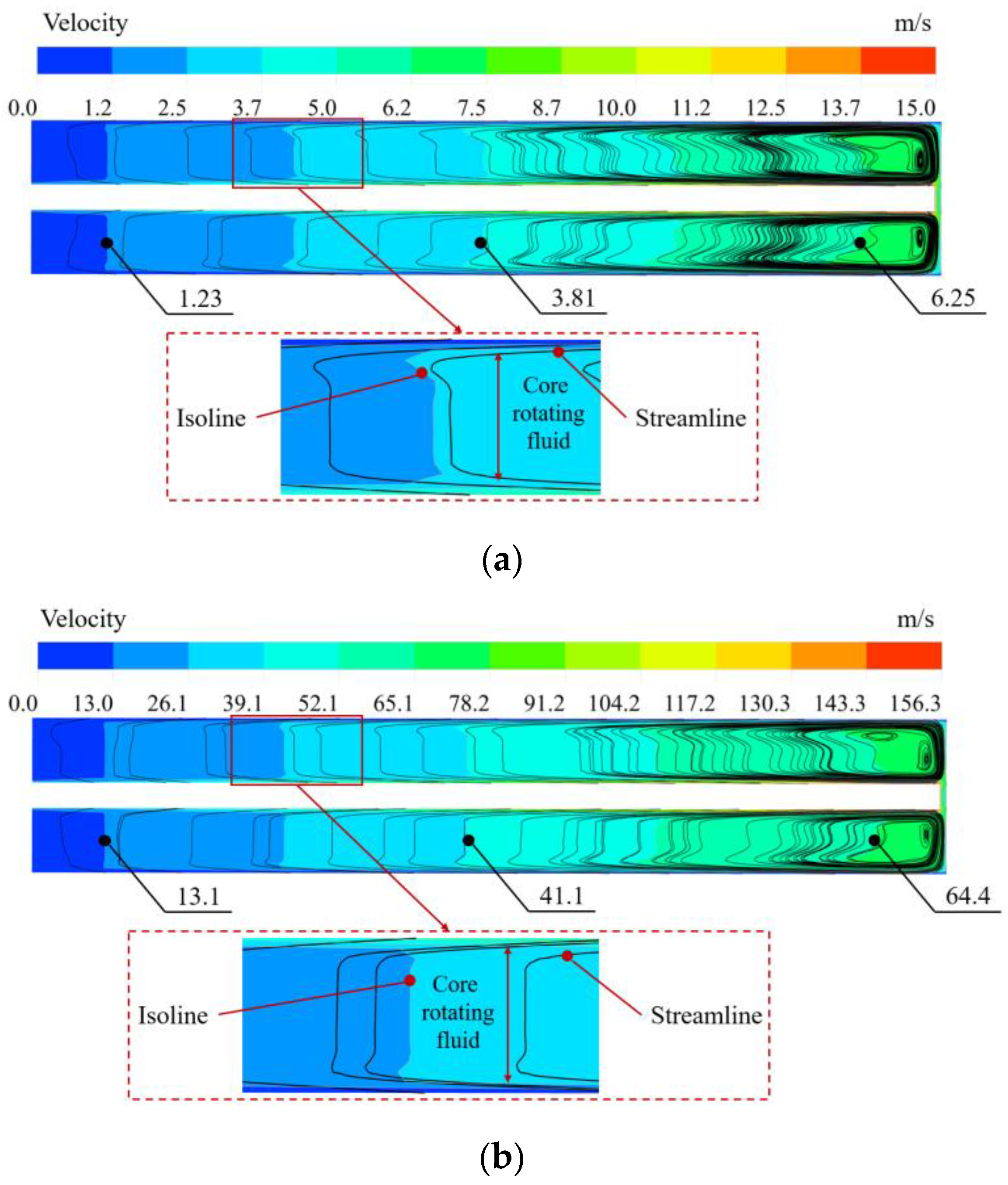
The following analyzes the causes of the deviation from the perspective of the flow in the gap. Figure 8 shows the velocity distribution of the flow in the gap of the cross-section (section of the fluid domain along the radial direction). It can be seen that due to the small S/R0 of Geometry 1, when Re = 4.06 × 10⁵, there is a velocity gradient between the boundary layer and the core rotating fluid of the rotor and stator. The boundary between the two regions is not obvious. The flow in the gap is approximately a Couette flow and the velocity is linearly distributed. With the increase of Re, it can be seen from Figure 8b,c that as the centrifugal force of the fluid near the wall increases, the viscous force decreases which leads to the increase of velocity gradient and the decrease of boundary layer thickness. According to the non-slip boundary condition, the fluid velocity near the rotor and stator wall is consistent with its corresponding velocity. At the position near the shaft (Re = 3.77 × 10⁶, R/R0 = 0.2), the velocity gradient difference between the boundary layers and the core rotating fluid at two Reynolds numbers is not alike. The boundary layers of the two walls convert from merging to separation. It can be predicted that with the increase of Re, the boundary layer separation phenomenon first appears in the low-velocity zone near the shaft and gradually expands along the radius direction until it covers the entire rotor surface, thus establishing the flow state of Region IV. What needs illustration is that for a sufficiently small size gap, there will be no boundary layer separation phenomenon.
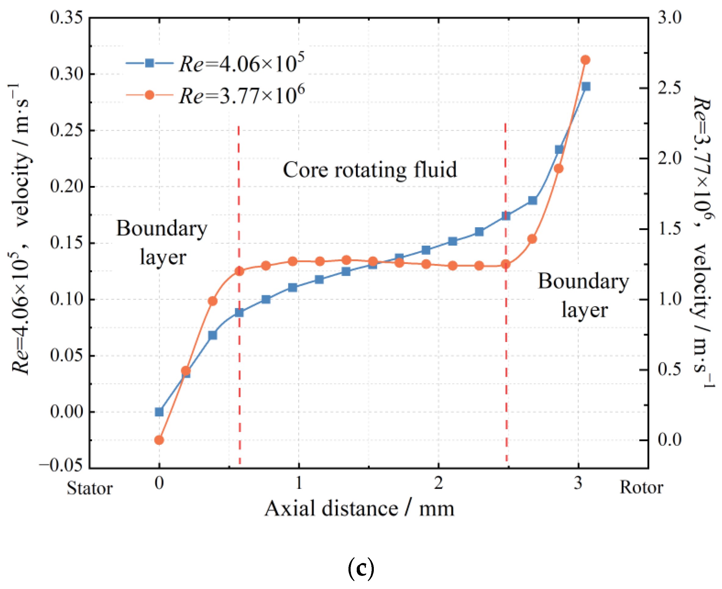
Figure 9 shows the circumferential velocity distribution of three radius ratio positions in the gap of Geometry 1 when the Reynolds number is 3.77 × 10⁶. It can be seen that the velocity distribution in the gap is basically the same at different radius ratios. In the boundary layer zones, the velocity gradient gradually increases along the radial direction, which is due to the wall boundary layer thinning. The velocity increases gradually along the radial direction, the centrifugal force of the fluid near the wall increases and the effect of the viscous force decreases. These make the boundary layer thickness near the wall decrease and the velocity gradient expand. In addition, when R/R0 = 0.5 and R/R0 = 0.8, the circumferential velocity of the core rotating fluid increases along the direction from stator to rotor, while at the position of R/R0 = 0.2, it decreases to a certain extent at R/R0 = 0.2.
Figure 10 is the velocity distribution and surface streamline in the gap of the cross-section. It can be seen that it is uncertain whether the boundary layer merging occurs for a larger S/R0 which may occur under the condition of a small Re. In addition, there is also radial flow. The core rotating fluid outside the boundary layers exerts different degrees of external excitation and radial pressure on the boundary layer of the rotor wall. The radial pressure makes the radial flow subject to the inverse pressure gradient, resulting in higher torque. The vortex near the end wall is formed as Re increases which makes the flow in this area lose stability. In addition, compared with Figure 8, with the increase of S/R0, the influence of wall velocity on the core rotating fluid and centrifugal force in the gap are weakened.
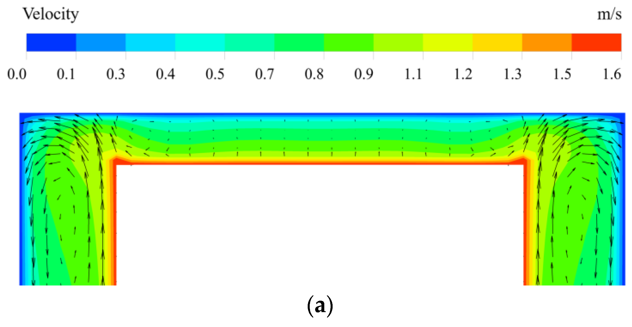
Figure 11 is the velocity vector in the rotor rim gap (end wall). The backflow phenomenon in the axial gap of the whole rim is not obvious (Re = 4.06 × 10⁵). The flow is similar to the annular Couette flow of the two rotating cylinders and basically shows the characteristics of laminar flow. When Re reaches 3.77 × 10⁶ (as shown in Figure 10b), multiple sets of vortex pairs appear in the rim and the annular Couette flow in the axial gap loses stability and forms a Taylor vortex [24]. It can be inferred that there is a critical Re between 4.06 × 10⁵ and 3.77 × 10⁶. When Re exceeds the critical value, the fluid pressure gradient will increase sharply and the instability will be enhanced.
In summary, the skin-friction coefficient model of Region III assumes that the boundary layers are merging which is mainly related to the flow on the rotor surface. It does not consider the influence of an unstable flow such as radial flow and Taylor vortex in the rim gap on the torque. In fact, an unstable flow occurs in the inlet and outlet parts of a gap behind the radial impeller. The size of the rim is not large and the influence on the windage loss of the whole back is not obvious.
4.2. Effects of Different Mediums
The main purpose of this section is to verify and study the accuracy of the skin-friction coefficient model of different mediums and the flow characteristics in the gap. In practical engineering applications, the geometric dimensions and boundary conditions of the radial impeller machinery are mainly concentrated in Region III and Region IV of the turbulent state; this section verifies 10 cases (as shown in Table 4) of these two regions.
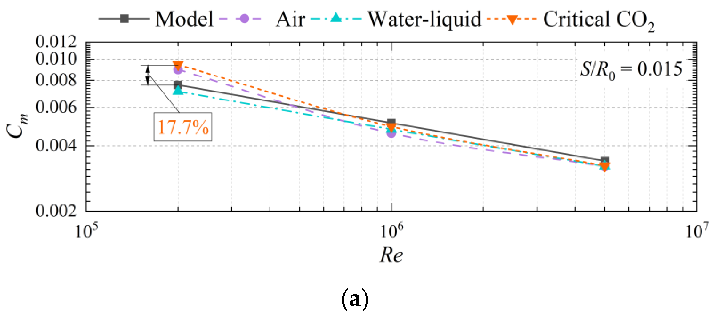
Figure 12 shows the comparison between the numerical calculation and the model prediction results of the three mediums with different relative gaps. The results in the figure have been repeatedly verified. As shown in Figure 12a, the relative deviation of the skin-friction coefficient calculated by the Region III model is greater than that of Region IV. The maximum relative deviation of air reaches −7.6% when the relative gap is 0.015 and the Region III deviation is negative. However, unlike the results of water, the relative deviation does not decrease with the increase of the relative gap. Overall, the relative deviations of the three mediums in Region IV are less than 2% and there is no regular change. The maximum relative deviation is 1.9% and the model prediction of Region IV is more accurate. The reason for the large model deviation in Region III may be related to the simultaneous boundary layer merging and separation in the gap. In Region IV with a higher Reynolds number, the boundary layer separation weakens the interaction between the rotor wall and the stator wall. The deviation rules of the three mediums are basically the same. It is worth mentioning that the relative deviation of critical CO2 is closer to that of water. The density and other physical properties of critical CO2 are significantly different from that of air.
When the relative gap changes, the velocity distribution and the gap working medium is air, as shown in Figure 13a,b. As mentioned above, when S/R0 = 0.005, the axial gap is very small and the boundary layers still merge together. When S/R0 increases to 0.025, the boundary layers first separate from the shaft and gradually diffuse along the radial direction. Figure 13c shows the vorticity distribution in the gap cross-section under the condition of air and critical CO2 (Region III, S/R0 = 0.015). By controlling the different rotational speeds, the Reynolds numbers in the two cases are the same. It can be seen that the vorticity of critical CO2 is greater. Under the conditions of two mediums, high vorticity zones appear near the rim of the end wall. In the rotor different zone, the vorticity distribution of the two mediums is diverse. This may be the reason for the large relative deviation of the air medium.
Compared with the relative gap, the influence of the Reynolds number on the windage loss in the gap is more intuitive and effective. The rotational speed of the rotor will make the centrifugal force of the fluid stronger which will have a great influence on the flow of the fluid in the gap. When the Reynolds number is high, the influence of the end wall flange on the flow in the gap will be more significant. When the Reynolds number changes, Figure 14 shows the comparison results of the numerical calculation and model prediction of three mediums under different Reynolds numbers in Region III and Region IV.
Similar to the cases of different relative gaps, the relative deviation of Region III is still large at different Reynolds numbers in the gap. The maximum relative deviation of critical CO2 reaches 17.7% when the Reynolds number is 2.0 × 10⁵. The relative deviation has no positive or negative regular pattern but decreases with the increase of the Reynolds number. In Region IV, the relative deviation has no regular changes. Only when the Reynolds number is 1.0 × 10⁸, the relative deviation is greater than 1% and the relative deviation of air is 6.6%. In fact, in the experiment of Ref. [3], the cases of Reynolds numbers greater than 107 are not included. Therefore, the decrease in model accuracy under high Reynolds numbers is tolerable.
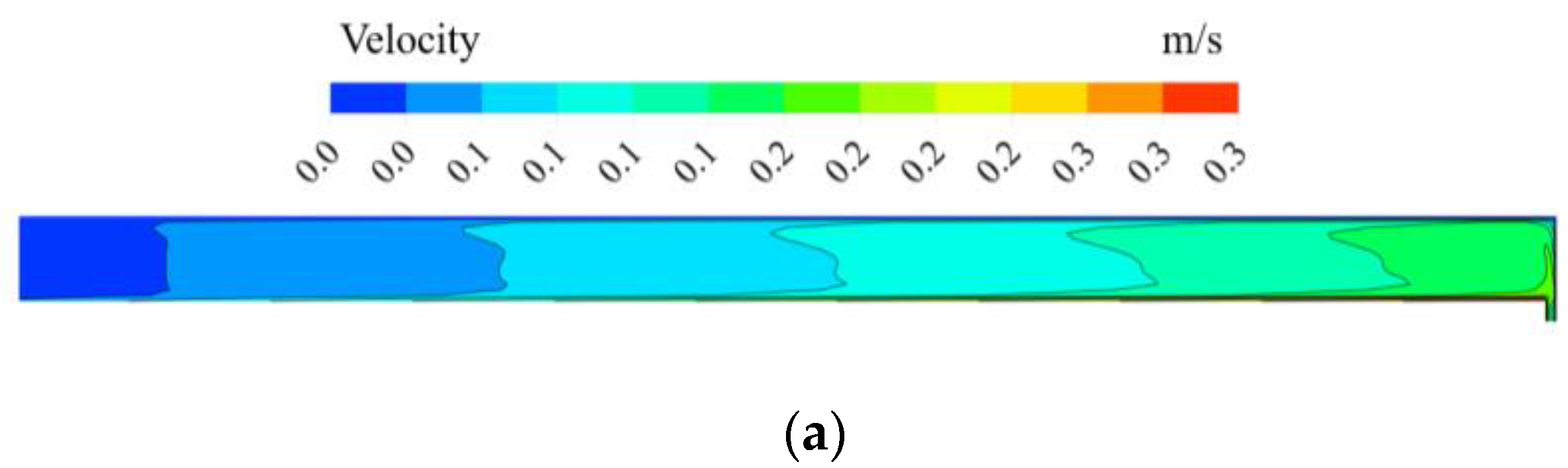
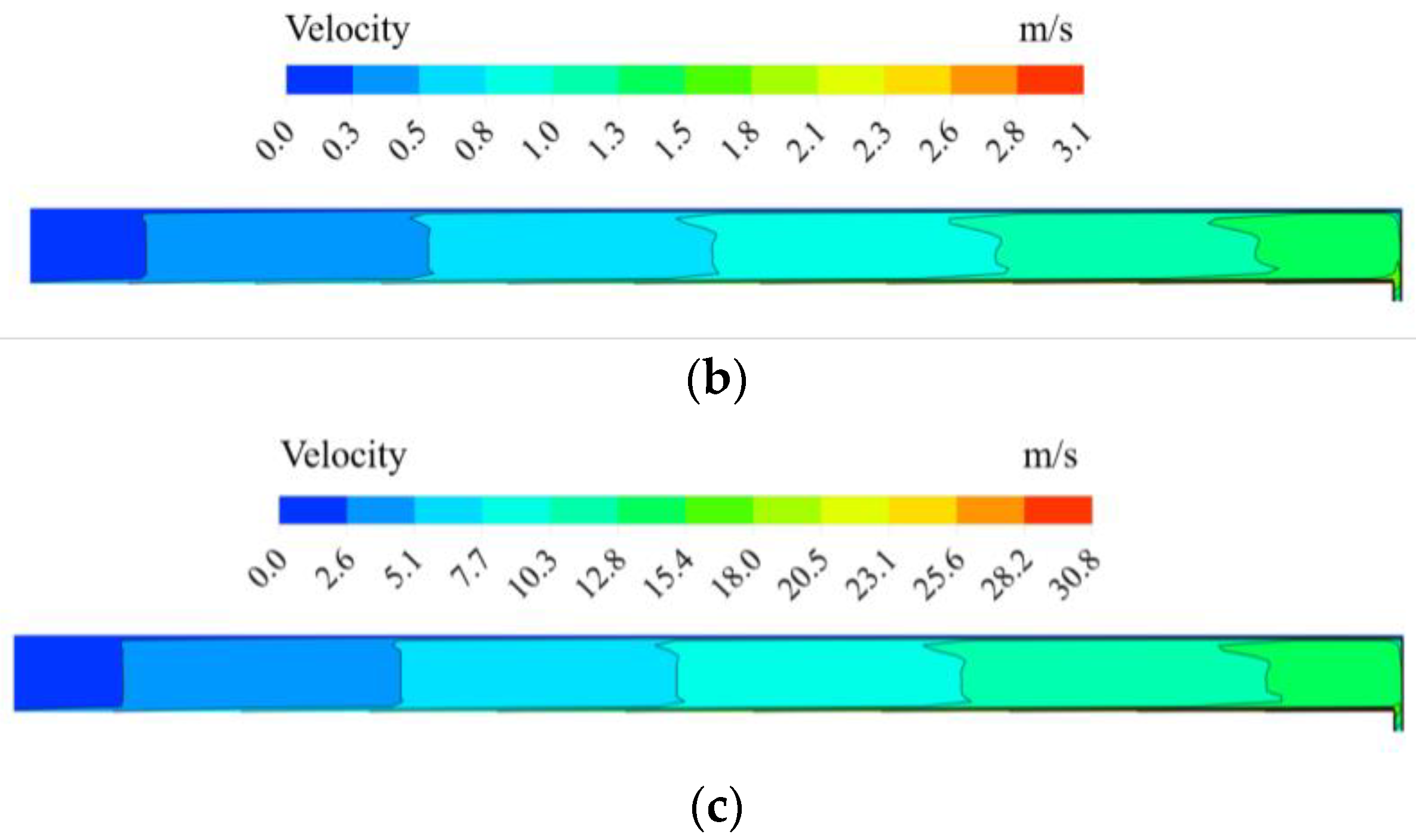
Figure 15 shows the circumferential velocity distribution at two Reynolds numbers (Re = 2 × 10⁵, 5 × 10⁶). As shown in the figure, the velocity distribution in the gap can be divided into three zones. They are the velocity drop and rise zones in the two wall boundary layers and the velocity stable zone in the core fluid. The higher Reynolds number will lead to the increase of the velocity gradient in boundary layers and there is also a higher velocity gradient in the corresponding velocity stable zone. Figure 16 shows the contour of velocity distribution in the gap of Region IV. At high Reynolds numbers, it can be seen that as the Reynolds number increases, the velocity in the gap increases and the velocity distribution tends to be uniform. The tips of the velocity move inward which is consistent due to the thinning of the boundary layers between the rotor wall and stator wall.
It is worth mentioning that the conclusion has been drawn that when the Reynolds number is near 107 and below, the precision of the skin-friction coefficient model in Region IV is very high. Combined with the above research, it can be concluded that in Region III, with the increase of the relative gap and Reynolds number, the model becomes more and more accurate when the working point is closer to Region IV. This provides a direction for the aerodynamic design and structural design of radial inflow turbomachinery in practical engineering applications. In the design of standard operating conditions, the Reynolds number can be selected concerning the range mentioned above. The corresponding Reynolds number range can also be referred to the structural design. The power loss of turbomachinery is obtained by a more accurate model to guide the aerodynamic design.
4.3. Prediction Method of Optimum Gap
In the radial impeller machinery, the axial gap loss behind the impeller is similar to the above research object. However, it is only a unilateral gap. When the flow in the gap is laminar, the skin-friction coefficient increases with the decrease of the gap size in Region I. The experimental and numerical results in Ref. [3] show that when the Reynolds number is constant, the skin-friction coefficient decreases first and then increases with the decrease of the gap. Therefore, based on the skin-friction coefficient model of Region III and Region IV, this paper proposes a method to predict the optimal gap of the radial impeller to minimize the windage loss [25]. The calculation formula is as follows:
The impeller parameters of the supercritical carbon dioxide (sCO2) unit designed by Sandia National Laboratory [26] are shown in Table 5. It should be noted that the parameters such as the impeller inlet pressure and temperature in the table are obtained according to the thermodynamic design and analysis program of the centripetal turbine of the research group. The accuracy of the program is verified and reliable and is used as the known flow parameters in the gap behind the impellers.
Figure 17 shows the relationship between the skin-friction coefficient and the relative gap in Region III and Region IV under the turbine parameters in Table 5 and the working medium is CO2. For the turbine parameters in Table 5, the curve is obtained by a fixed Reynolds number of 1.86 × 10⁷. It can be seen that when the Reynolds number is constant, according to the theoretical model, the skin-friction coefficient decreases with the increase of the relative gap in Region III. When the flow falls into Region IV, the skin-friction coefficient increases with the increase of the relative gap. The optimal relative gap covering the two flow regions is 0.0176 (the corresponding axial gap behind the impeller is 0.6 mm). Since the back of the impeller has only a single surface, the corresponding minimum skin-friction coefficient is 0.0012 and the windage loss at this time is 0.897 kW. Similarly, the optimum relative gap of the compressor is 0.0156 (the corresponding axial gap behind the impeller is 0.3 mm), the minimum skin-friction coefficient is 0.00104 and the windage loss is 0.307 kW.
Since the gap size of the turbine and the compressor designed by the Sandia laboratory is unknown, it is assumed that the optimal relative gap is adopted. Figure 17 shows the optimal gap by using turbine parameters; in order to verify whether the windage loss is the smallest under the optimal gap condition, two cases are taken before and after the optimal gap value. The boundary conditions are consistent with the parameters in Table 5. The optimal gap verification results are shown in Table 6. The windage loss obtained by the S/R0 = 0.0172 and 0.0180 is greater than the optimal gap.
The windage loss of the gap behind the impeller between the sCO2 turbine and the compressor is numerically verified. The boundary conditions are from Table 5. The final results are shown in Table 7. It can be seen that the numerical calculation results are greater than the model prediction results and the deviation is less than 5%. The theoretical model is still reliable when CO2 is used as the medium and less than the deviation when water is used.
Figure 18 shows the velocity distribution in the gaps behind the turbine and compressor impellers. Due to the high Reynolds number of the two cases, the boundary layer separation of the two walls still occurs although the axial gap is small. When the medium is CO2, the viscosity near the critical point is low and the influence of the boundary layer on the flow loss is reduced. In addition, the different working temperatures of the turbine and the compressor make a difference in the viscosity coefficient. The friction torque on the rotating disk is proportional to the viscosity coefficient, so the deviation between the turbine and compressor is also different. It should be noted that there is a discrepancy in the ratio of the inner and outer diameters of the impeller between the two, with different relative areas of the impeller back surface, which is one of the reasons for the deviation.
Through the verification of this paper, the prediction method of the optimal gap has good applicability for water-liquid and CO2 working fluids. The optimal gap obtained by this method will provide a basis for the design of a radial turbine structure. It should be noted that once the structure is manufactured, it may not be at the optimal gap when operating under variable conditions. The windage loss of the gap is the smallest under the design condition. Since the method is based on the model of two regions of the turbulent state, it has higher applicability in the range of Reynolds numbers from 1.58 × 10⁵ to 108. In fact, in radial turbomachinery such as the supercritical carbon dioxide cycle, the windage loss of the gap behind the impeller is greater than the current predicted value. The main reasons are as follows: (1) The size value of the gap is greater than the predicted value due to the axial expansion of the rotor and the axial movement; (2) There are generally deduplication pits on the back side of the impeller and the back side is not completely circumferentially smooth; (3) The existence of the inlet and outlet in the gap causes the flow to have a certain radial flow which is different from the hypothesis of the prediction model; (4) The temperature distribution of the impeller and stator will affect the flow and the ratio of the temperature of the gap to the temperature of the flow also has a great influence on the distribution of the heat transfer [27].
However, in the design of such radial turbomachinery, the best gap size can be obtained according to the flow parameters at the gap between the impeller and the guide blade and the prediction model of Region III and Region IV. Through certain structural design measures, the best gap can be as close as possible to minimize the windage loss of the gap behind the impeller.
5. Conclusions
In this paper, the skin-friction coefficient model of windage loss in a rotor–stator gap is verified and the influence patterns of gap size, Reynolds number and medium type on the skin-friction coefficient model are clarified. A method for predicting the optimal gap behind the radial impeller is proposed. The main conclusions are as follows:
- The effects of the relative gap on the two turbulent state skin-friction coefficient models are studied. The results show that the relative deviation between numerical calculation and model prediction results decreases with the increase of relative gap and the maximum deviation is −12.4% when the relative gap is 0.0127. The area occupied by the core rotating fluid outside the boundary layers increases which increases the skin-friction coefficient of the rotor surface. The model of Region III assumes boundary layer merging. In fact, there are two states of boundary layer merging and separation in the flow of Region III, so the model accuracy of Region III is lower than that of Region IV.
- As the Reynolds number increases, the skin-friction coefficient decreases gradually. Since the windage loss is positively correlated with the third power of the rotational speed, windage loss actually increases. In addition, at higher Reynolds numbers, the prediction results of the boundary layer separation state are more accurate and the maximum deviation is only 6.1%. The boundary layers of the rotor and stator wall transfer from merging to separation resulting in a larger velocity gradient and higher skin-friction coefficient near the wall. The model of the boundary layer merging state still has the state of separation. Since the Reynolds number is higher than 107 and has not been experimentally corrected, the accuracy of the Region IV model decreases at higher Reynolds numbers.
- The accuracy of the two turbulent state models under three mediums of air, water-liquid and critical CO2 was studied. Due to the difference in physical properties, the vorticity distribution of air and critical CO2 is diverse in the gap. The results show that when the physical properties of the medium change, the accuracy of the model of boundary layer separation state at low Reynolds number decreases, but all show a trend of decrease in the process of transition from merging to separation. The model accuracy of the remaining states is not sensitive to the change in the physical properties of the working medium.
- According to the two turbulent state models, a method for predicting the optimal gap behind the radial impeller is proposed which is verified on the sCO2 principle prototype of the Sandia National Laboratory in the United States. The theoretical optimal gap size is obtained and verified by numerical calculation. The results show that the theoretical model is still reliable when the working fluid becomes sCO2. However, since the method is aimed at the optimal gap under a fixed Reynolds number, the windage loss obtained by this method under the design condition is the smallest. When the structural design of the turbine is completed, the optimal gap under variable conditions is different from the design condition. In addition, the difference between actual windage loss and theoretical loss is analyzed and four aspects that need to be paid attention to in the further development of high-precision windage loss models are pointed out.
Author Contributions
Conceptualization, Z.Z. and Q.D.; software, Z.Z.; investigation, Z.Z.; data curation, L.H.; writing—original draft preparation, Z.Z.; writing—review and editing, J.L. and Z.F.; visualization, Z.Z. and L.H.; supervision, Q.D. All authors have read and agreed to the published version of the manuscript.
Funding
This research was funded by Joint Funds of the National Natural Science Foundation of China: U20A20303 and National Key R&D Program of China: 2017YFB0601804.
Institutional Review Board Statement
Not applicable.
Informed Consent Statement
Not applicable.
Data Availability Statement
Not applicable.
Conflicts of Interest
The authors declare no conflict of interest.
References
- Fernando, K.; Thomas, K.; Aaron, R. Calculating windage losses: A review. In Proceedings of the ASME Turbo Expo 2022, GT2022-82570, Rotterdam, The Netherlands, 13–17 June 2022. [Google Scholar]
- Aglen, O. Loss calculation and thermal analysis of a high-speed generator. In Proceedings of the IEEE International Electric Machines and Drives Conference, Madison, WI, USA, 9 July 2003; Volume 2, pp. 1117–1123. [Google Scholar]
- Daily, J.; Nece, R.E. Chamber dimension effects on induced flow and frictional resistance of enclosed rotating discs. J. Basic Eng. 1960, 82, 217–230. [Google Scholar] [CrossRef]
- Saari, J. Thermal Analysis of High-Speed Induction Machines. Ph.D. Thesis, Helsinki University of Technology, Espoo, Finland, 1998. [Google Scholar]
- Sirigu, S.A.; Gallizio, F.; Giorgi, G.; Bonfanti, M.; Bracco, G.; Mattiazzo, G. Numerical and Experimental Identification of the Aerodynamic Power Losses of the ISWEC. J. Mar. Sci. Eng. 2020, 8, 49. [Google Scholar] [CrossRef]
- Oh, H.W.; Yoon, E.S.; Chung, M.K. An optimum set of loss models for performance prediction of centrifugal compressors. Proc. Inst. Mech. Eng. Part A J. Power Energy 1997, 211, 331–338. [Google Scholar] [CrossRef]
- Hermann, S.; Klaus, G. Boundary-Layer Theory; Springer: Berlin/Heidelberg, Germany, 2016. [Google Scholar]
- Debuchy, R.; Abdel Nour, F.; Naji, H.; Bois, G. Investigation of the fluid flow in an isolated rotor-stator system with a peripheral opening. Sci. China Phys. Mech. Astron. 2013, 56, 745–754. [Google Scholar] [CrossRef]
- Crespi, F.; Gavagnin, G.; Sánchez, D.; Martínez, G.S. Supercritical carbon dioxide cycles for power generation: A review. Appl. Energy 2017, 195, 152–183. [Google Scholar] [CrossRef]
- Gülich, J.F. Disk friction losses of closed turbomachine impellers. Forsch. Ing. 2003, 68, 87–95. [Google Scholar] [CrossRef]
- Nemdili, A.; Hellmann, D.H. Development of an empirical equation to predict the disc friction losses of a centrifugallp pump. In Proceedings of the 6th International Conference on Hydraulic Machinery and Hydrodynamics, Timisoara, Romania, 22–24 November 2004; pp. 235–240. [Google Scholar]
- Nemdili, A.; Hellmann, D.H. Investigations on fluid friction of rotational disks with and without modified outlet sections in real centrifugalpump casings. Forsch. Ing. 2007, 71, 59–67. [Google Scholar] [CrossRef]
- Zhou, L.S.; Feng, Q.; Wu, Y.Y. Experiment on the velocity of the flow inside rotating disk cavity under mid rotating speed. J. Propuls. Technol. 2006, 27, 321–325. [Google Scholar]
- Cho, L.; Lee, S.; Cho, J. Use of CFD Analyses to Predict Disk Friction Loss of Centrifugal Compressor Impellers. Trans. Jpn. Soc. Aeronaut. Space Sci. 2012, 55, 150–156. [Google Scholar] [CrossRef]
- Darvish, D.M.; Nejat, A. Numerical investigation of fluid flow in a rotor–stator cavity with curved rotor disk. J. Braz. Soc. Mech. Sci. Eng. 2018, 40, 180. [Google Scholar] [CrossRef]
- Owen, J.M. An Approximate Solution for the Flow between a Rotating and a Stationary Disk. J. Turbomach. 1989, 111, 323–332. [Google Scholar] [CrossRef]
- Childs, P. Flow in Rotating Components-Discs, Cylinders and Cavities; Report; University of Sussex: Brighton, UK, 2007. [Google Scholar]
- Deng, Q.H.; Hu, L.H.; Zhao, Y.M.; Yang, G.Y.; Li, J.; Feng, Z.P. Windage Loss Model Verification and Flow Characteristic Analysis in Shaft-Type Gap. J. Xi’an Jiaotong Univ. 2022, 56, 54–63. [Google Scholar]
- Zheng, S.Y.; Wei, M.S.; Hu, C.X.; Song, P.P.; Tian, R. Flow characteristics of tangential leakage in a scroll compressor for automobile heat pump with CO2. Sci. China Technol. Sci. 2021, 64, 971–983. [Google Scholar] [CrossRef]
- Hu, L.H.; Deng, Q.H.; Yang, G.Y.; Li, J.; Feng, Z.P. Flow Characteristics and Windage Loss of CO2 in Shaft-type Rotor-stator Gap. J. Eng. Thermophys. 2022, 43, 647–655. [Google Scholar]
- Poullikkas, A. Surface Roughness Effects on Induced Flow and Frictional Resistance of Enclosed Rotating Disks. J. Fluids Eng. 1995, 117, 526–528. [Google Scholar] [CrossRef]
- Aungier, R.H. Centrifugal Compressors: A Strategy for Aerodynamic Design and Analysis; ASME Press: New York, NY, USA, 2000. [Google Scholar]
- Celik, I.B.; Ghia, U.; Roache, P.J. Procedure for Estimation and Reporting of Uncertainty Due to Discretization in CFD Applications. J. Fluids Eng. 2008, 130, 078001. [Google Scholar]
- Adebayo, D.S.; Rona, A. Numerical Investigation of the Three-Dimensional Pressure Distribution in Taylor Couette Flow. ASME J. Fluids Eng. 2017, 139, 111201. [Google Scholar] [CrossRef]
- Deng, Q.H.; Zhao, Z.B.; Hu, L.H.; Li, J.; Feng, Z.P. A High-Precision Prediction Method of Friction Loss in Back Clearance of Impeller. China National Invention Patent CN202210265888.6, 3 June 2022. [Google Scholar]
- Wright, S.A.; Radel, R.F.; Vernon, M.E.; Pickard, P.S.; Rochau, G.E. Operation and Analysis of a Supercritical CO2 Brayton Cycle; Sandia National Laboratories: Albuquerque, NM, USA; Livermore, CA, USA, 2010. [Google Scholar]
- Liao, G.L.; Wang, X.J.; Li, J.; Zhou, J.F. Numerical investigation on the flow and heat transfer in a rotor-stator disc cavity. Appl. Therm. Eng. 2015, 87, 10–23. [Google Scholar] [CrossRef]
Figure 1.
Flow state region division [3].
Figure 1.
Flow state region division [3].

Figure 2.
Schematic view of the geometry.

Figure 3.
Verification points and their distribution.

Figure 4.
Comparison between Region IV model and experimental results [3].
Figure 4.
Comparison between Region IV model and experimental results [3].

Figure 5.
Turbulence model validation [3].
Figure 5.
Turbulence model validation [3].

Figure 6.
Grid-independence verification. (a) Mesh of the computational domain. (b) Circumferential velocity distribution (R/R0 = 0.5, Re = 2.91 × 10⁷). (c) 3.27 million grid solution with discretization error (R/R0 = 0.5, Re = 2.91 × 10⁷).
Figure 6.
Grid-independence verification. (a) Mesh of the computational domain. (b) Circumferential velocity distribution (R/R0 = 0.5, Re = 2.91 × 10⁷). (c) 3.27 million grid solution with discretization error (R/R0 = 0.5, Re = 2.91 × 10⁷).


Figure 7.
Results at different relative gaps.

Figure 8.
Velocity distribution of Geometry 1 at different Re. (a) Re = 4.06 × 10⁵. (b) Re = 3.77 × 10⁶. (c) Circumferential velocity distribution at R/R0 = 0.2.
Figure 8.
Velocity distribution of Geometry 1 at different Re. (a) Re = 4.06 × 10⁵. (b) Re = 3.77 × 10⁶. (c) Circumferential velocity distribution at R/R0 = 0.2.


Figure 9.
Circumferential velocity distribution of Geometry 1 at different R/R0.

Figure 10.
Contour of Geometry 3 velocity magnitude distribution. (a) Re = 3.77 × 10⁶. (b) Re = 3.93 × 10⁷.
Figure 10.
Contour of Geometry 3 velocity magnitude distribution. (a) Re = 3.77 × 10⁶. (b) Re = 3.93 × 10⁷.

Figure 11.
Contour of Geometry 1 velocity magnitude distribution at the end wall rim gap. (a) Re = 4.06 × 10⁵. (b) Re = 3.77 × 10⁶.
Figure 11.
Contour of Geometry 1 velocity magnitude distribution at the end wall rim gap. (a) Re = 4.06 × 10⁵. (b) Re = 3.77 × 10⁶.


Figure 12.
Comparison of various mediums with different S/R0. (a) Region III. (b) Region IV.

Figure 13.
Velocity and vorticity distribution in the gap. (a) Velocity distribution in the gap of S/R0 = 0.005 (Region III, air, Re = 1.0 × 10⁶). (b) Velocity distribution in the gap of S/R0 = 0.025 (Region III, air, Re = 1.0 × 10⁶). (c) Vorticity distribution in the gap under different mediums (S/R0 = 0.015, Re = 1.0 × 10⁶).


Figure 14.
Comparison of various mediums with different Re. (a) Region III. (b) Region IV.


Figure 15.
Circumferential velocity distribution at R/R0 = 0.5 (S/R0 = 0.015).

Figure 16.
Contour of critical CO2 velocity magnitude distribution in the gap (S/R0 = 0.05). (a) Re = 1.0 × 10⁶. (b) Re = 1.0 × 10⁷. (c) Re = 1.0 × 10⁸.
Figure 16.
Contour of critical CO2 velocity magnitude distribution in the gap (S/R0 = 0.05). (a) Re = 1.0 × 10⁶. (b) Re = 1.0 × 10⁷. (c) Re = 1.0 × 10⁸.


Figure 17.
Relationship between Cm of the relative gap behind the turbine impeller.

Figure 18.
Contour of velocity distribution of the gaps behind the turbine and compressor.


Table 1.
Cm models of the four flow regions [3].
Table 1.
Cm models of the four flow regions [3].
| Region | Equation | Flow State |
|---|---|---|
| Region I | laminar | |
| Region II | laminar | |
| Region III | turbulent | |
| Region IV | turbulent |
.
Table 2.
Parameters of geometric model.
| Parameters/mm | Geometry 1 | Geometry 2 | Geometry 3 | Section 4.2 |
|---|---|---|---|---|
| Relative gap S/R0 | 0.0127 | 0.0255 | 0.0636 | 0.005~0.065 |
| Axial length S | 3.18 | 6.35 | 15.85 | 1.25~16.20 |
| Outer radius R0 | 249.20 | |||
| Inner radius Ri | 25.40 | |||
| Gap width t | 6.35 | |||
| Rim gap c | 1.60 | |||
Table 3.
Parameters for boundary conditions.
| Parameters | Units | Water-Liquid | Air | Critical CO2 |
|---|---|---|---|---|
| Temperature | K | 298.15 | 304.13 | |
| Pressure | MPa | 0.1 | 7.38 | |
| Density | kg/m3 | 998.2 | 1.17 | 345.4 |
| Dynamic viscosity | Pa·s | 1.003 × 10⁻³ | 1.85 × 10⁻⁵ | 2.65 × 10⁻⁵ |
| Re | - | 2.0 × 10⁵~1.0 × 10⁸ | ||
Table 4.
Boundary conditions of different mediums.
| Region | Relative Gap (S/R0) | Re |
|---|---|---|
| Region III | 0.005 | 1.0 × 10⁶ |
| 0.015 | 2.0 × 10⁵, 1.0 × 10⁶, 5.0 × 10⁶ | |
| 0.025 | 1.0 × 10⁶ | |
| Region IV | 0.035 | 1.0 × 10⁷ |
| 0.050 | 1.0 × 10⁶, 1.0 × 10⁷, 1.0 × 10⁸ | |
| 0.065 | 1.0 × 10⁷ |
Table 5.
Parameters of sCO2 turbine and compressor from Sandia, Albuquerque, NM, USA [26].
Table 5.
Parameters of sCO2 turbine and compressor from Sandia, Albuquerque, NM, USA [26].
| Parameters | Units | Turbine | Compressor |
|---|---|---|---|
| Speed | r/min | 75,000 | 75,000 |
| Power rate | kW | 178 | 51 |
| Impeller outer radius | mm | 68.1 | 37.3 |
| Impeller inner radius | mm | 39.2 | 12.0 |
| Inlet temperature | K | 780.57 | 320 |
| Inlet pressure | kPa | 10,764.89 | 10,814 |
| Inlet density | kg/m3 | 72.13 | 543.02 |
| Kinetic viscosity | Pa·s | 3.54 × 10⁻⁵ | 4.16 × 10⁻⁵ |
| Re of gap | - | 1.86 × 10⁷ | 3.57 × 10⁷ |
Table 6.
Optimal gap verification results.
| Parameters | Value | ||
|---|---|---|---|
| Relative gap (S/R0) | 0.0172 | 0.0176 | 0.0180 |
| Loss model/kW | 0.956 | 0.897 | 0.961 |
| Numerical simulation/kW | 0.992 | 0.908 | 0.980 |
| Relative deviations | 3.8% | 1.2% | 2.0% |
Gray cells: optimal gap and corresponding results.
Table 7.
Parameters of sCO2 turbine and compressor from Sandia, USA.
| Results and Deviations | Turbine | Compressor |
|---|---|---|
| Loss model/kW | 0.897 | 0.307 |
| Numerical simulation/kW | 0.908 | 0.316 |
| Relative deviations | 1.2% | 2.9% |
Disclaimer/Publisher’s Note: The statements, opinions and data contained in all publications are solely those of the individual author(s) and contributor(s) and not of MDPI and/or the editor(s). MDPI and/or the editor(s) disclaim responsibility for any injury to people or property resulting from any ideas, methods, instructions or products referred to in the content. |
© 2023 by the authors. Licensee MDPI, Basel, Switzerland. This article is an open access article distributed under the terms and conditions of the Creative Commons Attribution (CC BY) license (https://creativecommons.org/licenses/by/4.0/).
Share and Cite
MDPI and ACS Style
Zhao, Z.; Deng, Q.; Hu, L.; Li, J.; Feng, Z. Skin-Friction Coefficient Model Verification and Flow Characteristics Analysis in Disk-Type Gap for Radial Turbomachinery. Appl. Sci. 2023, 13, 10354. https://doi.org/10.3390/app131810354
AMA Style
Zhao Z, Deng Q, Hu L, Li J, Feng Z. Skin-Friction Coefficient Model Verification and Flow Characteristics Analysis in Disk-Type Gap for Radial Turbomachinery. Applied Sciences. 2023; 13(18):10354. https://doi.org/10.3390/app131810354
Chicago/Turabian StyleZhao, Zhuobin, Qinghua Deng, Lehao Hu, Jun Li, and Zhenping Feng. 2023. "Skin-Friction Coefficient Model Verification and Flow Characteristics Analysis in Disk-Type Gap for Radial Turbomachinery" Applied Sciences 13, no. 18: 10354. https://doi.org/10.3390/app131810354
Note that from the first issue of 2016, this journal uses article numbers instead of page numbers. See further details here.