
System-Level Fault Diagnosis for an Industrial Wafer Transfer Robot with Multi-Component Failure Modes

1
Department of Aerospace and Mechanical Engineering, Korea Aerospace University, Goyang-si 10540, Republic of Korea
2
Department of Smart Air Mobility, Korea Aerospace University, Goyang-si 10540, Republic of Korea
3
Cymechs, Hwaseong-si 18487, Republic of Korea
4
School of Aerospace & Mechanical Engineering, Korea Aerospace University, Goyang-si 10540, Republic of Korea
*
Author to whom correspondence should be addressed.
Appl. Sci. 2023, 13(18), 10243; https://doi.org/10.3390/app131810243
Submission received: 20 July 2023
/
Revised: 1 September 2023
/
Accepted: 7 September 2023
/
Published: 12 September 2023
(This article belongs to the Special Issue Machine Condition Monitoring and Fault Diagnosis: From Theory to Application)
Abstract
:In the manufacturing industry, robots are constantly operated at high speed, which degrades their performance by the degradation of internal components, eventually reaching failure. To address this issue, a framework for system-level fault diagnosis is proposed, which consists of extracting useful features from the motor control signal acquired during the operation, diagnosing the current health of each component using the features, and estimating the associated degradation in the robot system’s performance. Finally, a maintenance strategy is determined by evaluating how well the system performance is restored by the replacement of each component. The framework is demonstrated using the example of a wafer transfer robot in the semiconductor industry, in which the robot is operated under faults with various severities for two critical components: the harmonic drive and the timing belt. Features are extracted for the motor signal using wavelet packet decomposition, followed by feature selection by considering the trendability and separability of the fault severity. An artificial neural network model and Gaussian process regression are employed for the diagnosis of the components’ health and the system’s performance, respectively.
1. Introduction
In the semiconductor industry, wafer transfer robots perform missions to move wafers from position to position. They are usually operated at very high speeds to accomplish high productivity while maintaining precise position control. Since the robot consists of several interconnected components such as the motor, speed reducer, timing belt, and so on, wear in these components occurs over time, which causes a degradation in the performance of the robot, and ultimately leads to the failure to perform its intended function. In the field, however, many manufacturing lines often rely on corrective maintenance, that is, the robots are kept in operation until failure, despite the fact that failure causes downtime of the entire line and a significant loss in productivity. Therefore, it is important to develop a solution to monitor the robot’s health condition to prevent such failures in a proactive way.
Many researchers have investigated this issue for industrial robots for decades. Kim et al. [1] proposed a fault detection method using vibration signals and phase-based time-domain averaging (PTDA) in the gearbox of an industrial robot. Capisani et al. [2] proposed a physical-model-based fault presence detection method. Yang et al. [3] proposed a data-based fault diagnosis method using the motor current signal of the ball screw. Cheng et al. [4] detected faults through unsupervised clustering learning for abnormal gears induced by removing grease artificially. Chen et al. [5] introduced a sliding window convolutional deformation autoencoder (SWCVAE) that can realize robot anomaly detection. While these papers have contributed significantly to the diagnoses of robot failures, their common limitation is that the object is a single component with binary fault conditions, which cannot capture the fault severity. Others, such as [6], diagnosed small, intermediate, and high gearbox backlash in a joint robot using DWT signal preprocessing and an ANN. Kim et al. [7] proposed a method to diagnose the severity of control cable wire damage. Huh et al. [8] diagnosed soft and hard pitting gears based on a critical information map (CIM). These studies improved diagnoses considering different fault severities, but studied only a single component, not multiple components.
In fact, a robot is composed of several components, each of which has their own failure modes. The issue of multiple fault diagnosis (MFD) has been addressed by several authors. Guo et al. [9] designed a level-based learning swarm optimizer–extreme learning machine (LLSO-ELM) model to further improve the generalization performance of ELM by combining it with LLSO, and classified a total of six failure modes for two components. Chen et al. [10] diagnosed five failure modes for three components by combining the generalized frequency response function (GFRF) spectrum and a convolutional neural network (CNN). Long et al. [11] proposed an attitude-data-based sparse auto-encoder–support vector machine (SAE-SVM) approach to diagnose transmission faults, implemented with eight failure modes for multi-joint industrial robots. Rohan et al. [12] diagnosed two failure modes, the wear of gear teeth and bearings, using motor current signature analysis (MCSA) with discrete wavelet transform (DWT) to analyze the signals in the time–frequency domain. In those studies, the drawbacks are that the faults are assumed to be mutually exclusive and are considered in a binary manner, i.e., normal and fault. However, failure modes of components can occur interactively, which complicates the problem and may lead to misleading results unless this is accounted for. This is also addressed in the recent paper by [13], in which the same challenge is stated for the PHM of industrial robots. In fields other than robotics, Qin et al. [14] proposed a methodology based on a multi-scale convolutional neural network–long short-term memory neural network (MSCNN-LSTMNet) to diagnose the failure of multi-cylinder diesel engines under interactive failure.
Summing up the above literature on industrial robots, the common finding is that most of the studies have focused on the diagnosis at the component level with faults of binary or multiple severities, and with regard to a single or multiple components. As mentioned in the beginning, the degradation of each component affects the performance of the robot system, not in an additive, but in an interactive manner. This means that the interrelation between the system and components should be accounted for, which we call diagnosis at the system level. In fact, the degradation of a component cannot be defined on its own but should be defined as conditional on the failure of the system, meaning that as long as the system performs its function well, the components have not yet failed.
Motivated by this issue, this paper proposes a procedure of how to conduct a system-level diagnosis for a system with multiple components. The method is demonstrated by applying it to a wafer transfer robot with two components, a harmonic drive (HD) and timing belt (TB), which are known as the most critical components responsible for robot failure [15]. To this end, a test rig is constructed, in which a robot is operated under various fault conditions with different severities. During the operation, the motor signal acquired to control its motion is exploited to diagnose the health of the system and its components. According to the robot company, the system performance is defined by a vibration magnitude of the end-effector during the operation, which is measured by an accelerometer. If the value exceeds a certain threshold, it is regarded as failure, that is, the robot fails to deliver the wafer to the target position, and the operation is aborted. In order to relate the motor control signal with the faults of the components, features are extracted by using the wavelet packet decomposition (WPD), which is known to be effective for nonstationary signals. A framework for system-level diagnosis is constructed, which enables the estimation of the current state of health of each component and the system performance. It consists of two models: the artificial neural network (ANN) for the diagnosis of component health and the Gaussian process regression (GPR) for the estimation of system health.
To summarize, the contributions of the proposed work are as follows: First, multiple components with multiple degradation severities are examined to perform fault diagnosis of the robots. Second, the method leverages motor control signals, which are acquired automatically during operation, eliminating the need for supplementary sensors. Third, a framework for system-level diagnosis is proposed, assessing the component health in relation to the system performance, which is contrasted to the conventional component-level strategies.
The rest of the paper is organized as follows: Section 2 presents the proposed methodology and theoretical background for the algorithms. Section 3 gives a brief explanation of the industrial wafer transfer robot and the designed experiment. Then, Section 4 presents the result of proposed methodology with the datasets of the designed experiment. Lastly, conclusions and potential future works are presented in Section 5.
2. Methodology
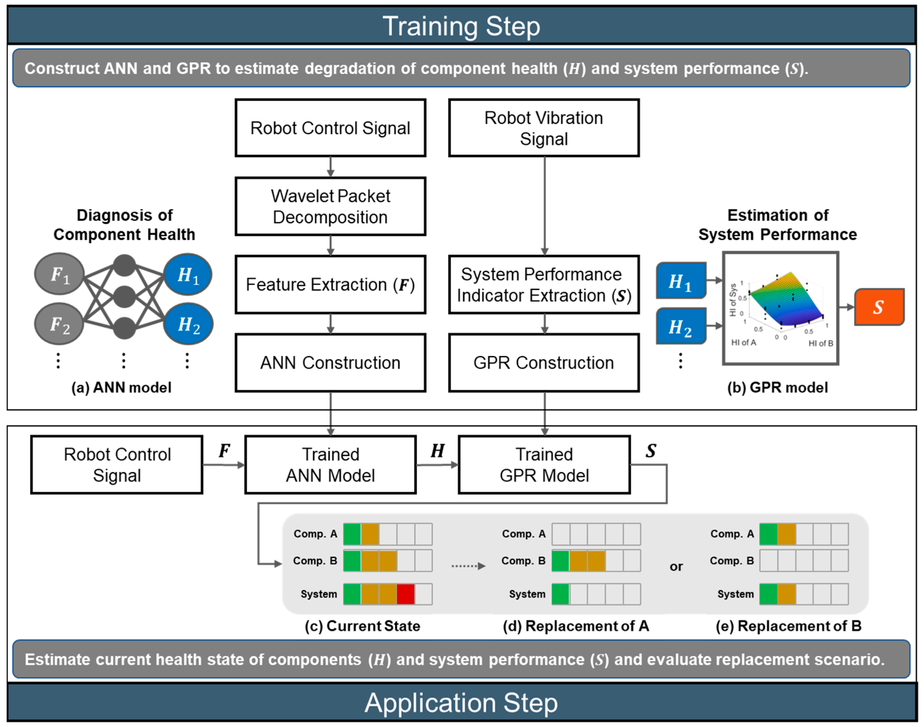
The proposed methodology is illustrated in Figure 1, which addresses the system-level diagnosis framework. It consists of two steps: (1) training and (2) application. In the model training, two models are constructed to estimate the health of each component () by using the features () from the motor control signal and to estimate the resulting degradation of the system performance ().
In order to construct the models, artificial faults of different severities are seeded into the components, and this can simulate the health degradation of each component, which is given by 1, 2, … in the figure. The robots are operated under each fault condition, during which the informative features are extracted and selected from the motor signals that control the motion. These are denoted by 1, 2, … in the figure. A vibration signal is also acquired from the end-effector by the accelerometer, by which the root mean square (RMS) values are computed as a measure of system performance. These are denoted by 1, 2, … in the figure. In the feature extraction, wavelet packet decomposition (WPD), which is appropriate for nonstationary signals, is employed, in which the signals are decomposed into the time–frequency domain. The statistical features and wavelet energy (WE) are extracted for each decomposed coefficient. A hybrid score based on the Spearman correlation and Fisher discriminant ratio (FDR) is then applied to select the most informative features among the features pool. Once the data are prepared by this method, the artificial neural network (ANN) model is constructed to relate the features set () with the health () of each component as shown in Figure 1a. A Gaussian process regression (GPR) model is also constructed to relate the health () of each component with the system performance () as shown in Figure 1b.
After the construction of the models, they are applied to diagnose the health of a new robot by using the motor control signal. Introducing the health indicator (HI) as 0 and 1 for the normal and failure, respectively, the results may be represented by a bar chart as in Figure 1c, which shows the current state of health of each component as well as the system performance. In this figure, they are given by 0.4, 0.6, and 0.8 for the components A, B, and system as an illustration. Note that the degradation of system performance stems from these components. Once this is available, one can further develop the replacement strategy by conducting a what-if study: if only the component A or B is replaced, i.e., the HI of A or B is restored to 0, then the HI of the system will be restored to 0.2 or 0.4 as shown in Figure 1d,e, respectively. In this illustration, it is better to replace A since the system restores to the better condition 0.2 than the alternative, 0.4. Note that simply replacing the worse component B in HI, which is illustrated in Figure 1e in this case, does not always result in the better restoration of system performance. This is because of the nonlinear and interactive nature of components and system in terms of health degradation, which is why the system-level diagnosis framework is necessary.
2.1. Feature Extraction by Wavelet Packet Decomposition
In the robot operation, the signals acquired from the motor are nonstationary. In this case, approaches based on the time–frequency domain such as the wavelet transform are more appropriate than those on the frequency domain such as the fast Fourier transform. In this study, wavelet packet decomposition (WPD) is employed for the purpose of feature extraction, which is briefly described as follows:
Wavelet packet consists of a set of linearly combined wavelet functions, which are generated using the following recursive relationship [16,17]:
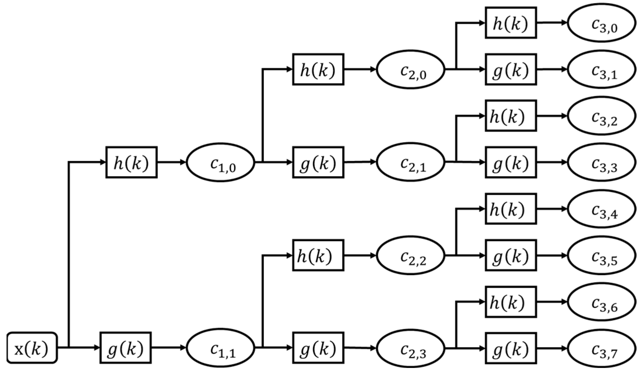
where is the scaling function, is the wavelet function, and is an integer from 0 to . Functions and represent coefficients of low-pass and high-pass filter of Quadrature mirror filters (QMF) which are related to each other by . For each step of the decomposition, the input signal is decomposed into approximation in low frequency and detail in high frequency, which is expressed recursively as:
where denotes the wavelet coefficients at the -th level, -th sub-frequency band. As a result, the original signal can be expressed as the sum of the coefficients as follows:
An example of a 3-level decomposition of the signal using the WPD is shown in Figure 2.
Given the decomposed coefficients, wavelet energy (WE) is extracted as a feature for each frequency band, which is defined as below.
2.2. Feature Selection
Among the extracted features, it is necessary to find the most informative ones for more efficient and accurate diagnostic performance. For this purpose, a score metric is introduced, which accounts for the two following aspects: First, the features should present a consistent trend as the fault severity rises, which is an important factor as the health indicator. Second, Spearman correlation (named here) is employed to evaluate this, which is defined as
where and denote the rank variables of feature and fault severity . The is calculated for each component. Next, the features should have good separability of the individual faults and their severities. This can be evaluated by the Fisher discriminant ratio (FDR) defined as follows:
where and represent the variances of between-class and within-class, respectively, in which each class denotes the individual fault with different severities.
By combining the two metrics, a hybrid score is defined for each component. For example, assume that we have three components A, B, and C, and we have acquired signals for each component under the fault conditions with the number of severities being , , and , respectively. For example, if , it means that the fault is applied to the component A with 4 severities: normal (no fault), small, medium, and large degree of fault. Then the total number of conditions is . For each fault condition, a large number of features is obtained by decomposing the signal through WPD and extracting the features. For an individual feature, the correlation of component A can be defined as
where represents the correlation of the feature with respect to the fault severity A when B and C are at the severity level and , respectively. Since this is performed for to and to to result in number of , these are summed to obtain a single representative value. Then the result is replaced by absolute value since the can be negative. The same process is applied to obtain to evaluate the separability of fault severity of component A, which is defined as
Once the two metrics and are calculated, they are combined into a single score by introducing weight parameter . Before proceeding, however, the metric values are normalized since they differ in scale. Min–max algorithm is applied to the whole features so that they vary within the interval [0, 1], by assigning 0 and 1 to the minimum and maximum values. Then, the hybrid score for component A is given by
where the symbol indicates the metrics are normalized by min–max algorithm. In this way, the score is calculated for all the components A, B, and C for each feature.
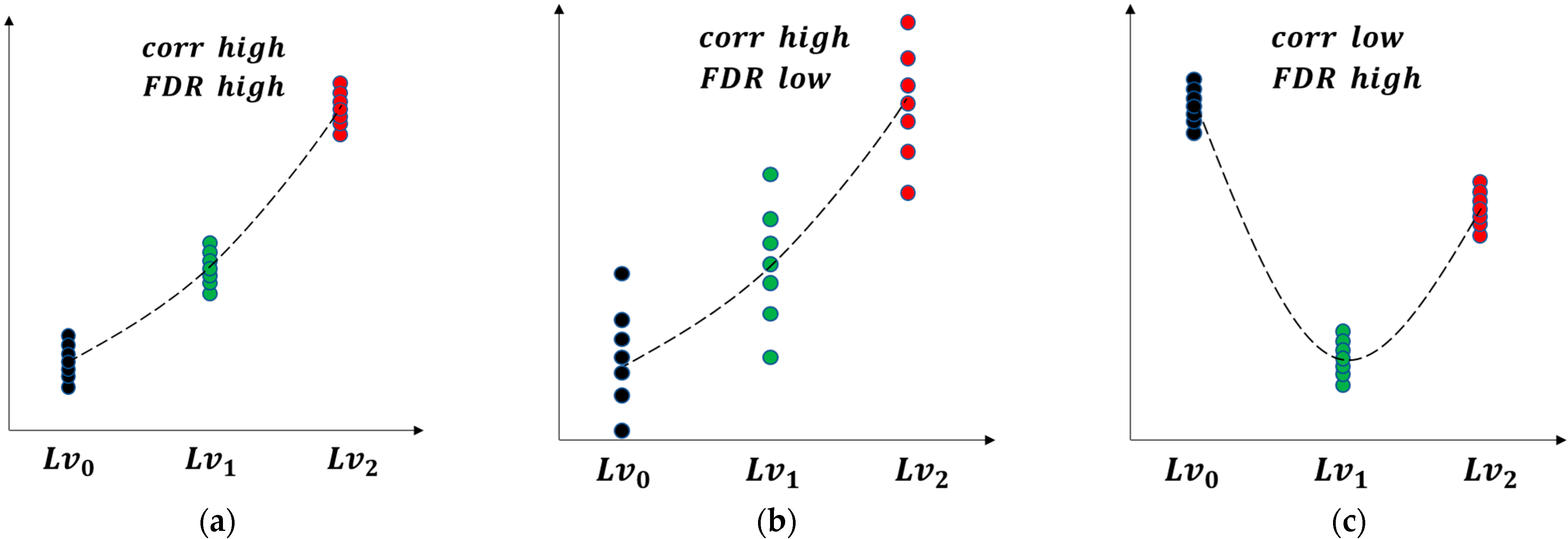
The reason why we need to consider the two metrics together is illustrated in Figure 3, which shows three cases where, in Figure 3a, is low but is high, in Figure 3b, is high but is low, and in Figure 3c, both are high. While Figure 3a shows high separability, it is less useful since it is not consistent with respect to the fault progression. Likewise, Figure 3b is also less useful due to the large variance, even though the is high. For this reason, the feature should have higher values in both metrics.
Once the score is obtained for all the features by using Equation (11), the next step is to select a few good features with a high score. While this can be performed arbitrarily, it is achieved in a more objective manner by applying the formula based on the risk priority number (RPN) threshold estimation [21]. The idea is to divide the whole features into negligible parts, characterized by a gradual change, and the significant part, with a steep increase in score. It was originally developed to select failure modes with highest RPN in the failure mode, effect, and criticality analysis (FMECA), but the authors believe that it is applicable here too. The process begins with setting a unique score and calculating the frequency of each score. The weighted finite difference is defined by dividing the finite difference by the frequency of the unique score as follows:
where is the index of the unique score. It indicates that the smaller the frequency of the unique score and the larger the finite difference, the larger the weighted finite difference and the greater the variation between the two consecutive values. Then, the peak, namely the local maxima, is obtained to indicate a significant increase in two consecutive unique scores, which is obtained by the following equations:
In the final step, maximum peak is identified and the corresponding score value is used as the threshold to identify the most significant features. Further details will be addressed in the subsequent case study.
Sometimes, the selected features are dependent on each other, that is, show a similar trend in terms of fault severity. An example is that of variance and standard deviation. In this case, the two are highly redundant and just one is enough to conduct the diagnosis. To this end, Pearson correlation is computed for pairs of features combination. If the value is close to 1, remove either one in the resulting features. Finally, one obtains the selection of features for each component that fulfills all the criteria: consistent trend, separability, and independency.
2.3. Model Construction
As mentioned in Figure 1, two models, ANN and GPR, are utilized for the diagnosis of component health and system performance, respectively. The reason for choosing these models is that they are established techniques, easy, and have been universally applied in the field of fault diagnosis for a long time.
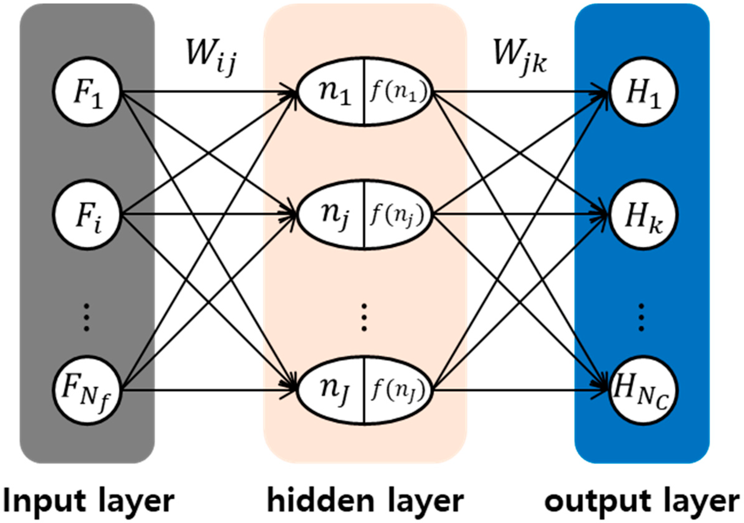
ANN and GPR are employed for the diagnosis of component health and the estimation of system health, respectively. ANN is widely used for data-driven diagnostics, since it can map various input variables onto the output data such as the health degradation. The structure of ANN is composed of an input layer, one or more hidden layers, and an output layer, as shown in Figure 4 [22]. Each layer contains neurons (nodes) and weights. In this paper, the set of selected features with dimension from the motor signal is used as the input and the degradation level of the components with dimension , which is the number of components, is given for the output. The ANN is trained using the data of and , acquired for various fault conditions, to determine the optimum weights that represent the nonlinear relationship between the input and output. To enhance the accuracy of ANN, the number of nodes in hidden layers are optimized through k-fold cross-validation.
The GPR is used to estimate the system health based on the fault severity of the components, which is identified by ANN. Denoting and by with the dimension as the number of components and , respectively, the GPR is represented by the global function and the covariance function as follows [23,24,25]:
where represents the Gaussian process. Generally, the covariance function consists of two parts, , where is the functional part, while is the noise part, which are given as follows:
where , and are hyperparameters associated with the scaling factor, length-scale, and noise variance that need to be estimated. Generally, these hyperparameters are optimized by maximizing the log-likelihood function, giving the training dataset, . The advantage of using GPR is that it cannot only represent the nonlinear relationship between input and output , but also provide the distribution of the function to quantify the uncertainty of the model or measurement by means of the confidence interval.
3. Wafer Transfer Robot System
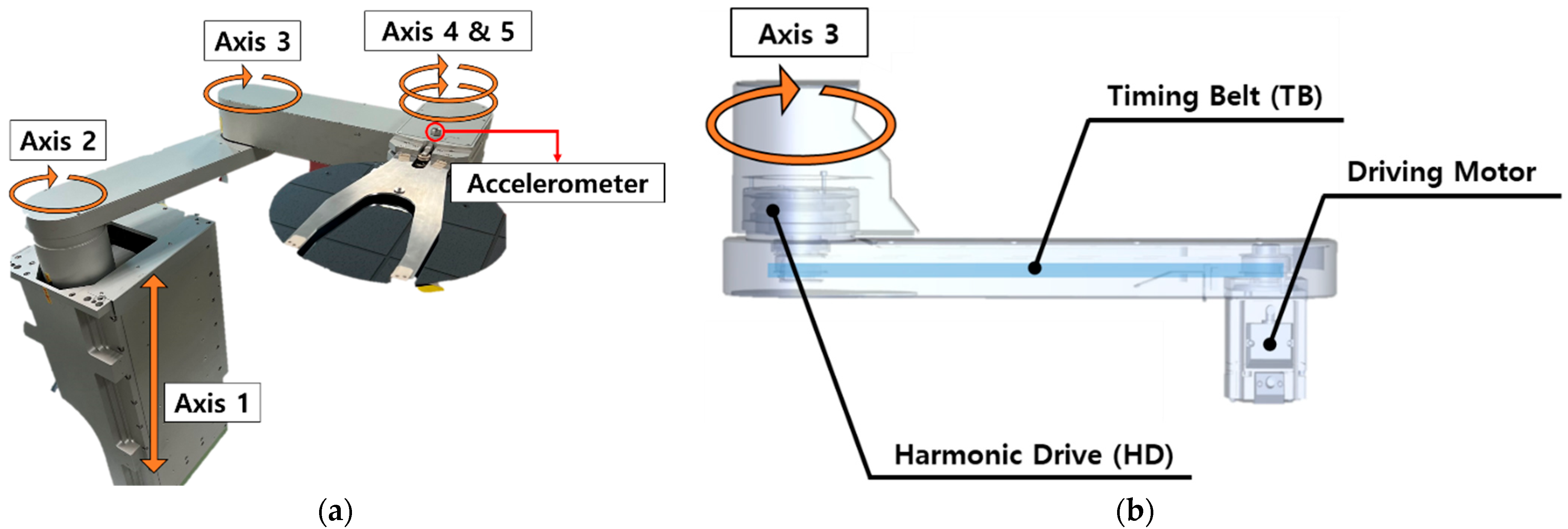
The wafer transfer robot in this study is a multi-joint structure robot with five axes, as shown in Figure 5a, in which vertical or rotating movement is generated with the power transmission components such as a ball screw, driving motor, timing belt, or harmonic drive. The robot is used to transport wafers to the load port module (LPM), which is a vacuum chamber for the semiconductor process. Axis 1 operates a vertical motion of the arm assembly by rotating the ball screw located at the bottom of the robot. Axes 4 and 5 rotate each end-effector individually to transport two wafers, while axes 2 and 3 are rotated to approach multiple LPMs.
Since the robots in the field are often operated at high speed without rest, the components undergo wear as time progresses, which degrades the position accuracy. This is, however, compensated by the control logic to adjust or increase the motor current so as to ensure the wafer delivery to the target location. Nevertheless, faults inside the system cause vibration at the end-effector and may even lead to the failure to deliver the wafer since the receiving slot is very narrow. This is why the company monitors the vibration in the z-direction when they evaluate the robot’s performance. A single axis accelerometer is mounted at the end-effector axis for this purpose, as shown in Figure 5a.
3.1. Target Components
According to surveys [26,27], the two most typical components responsible for the failure in the wafer transfer robot are the harmonic drive (HD), which is a type of speed reducer that accomplishes a high reduction ratio in a small space, and the timing belt (TB), which transmits the power to the remote location. In order to carry out the fault diagnosis of these components, axis 3, which is rotated by both the HD and the TB, as shown in Figure 5b, and controls the rotational motion of the axis 3 arm, is chosen as the object of study.
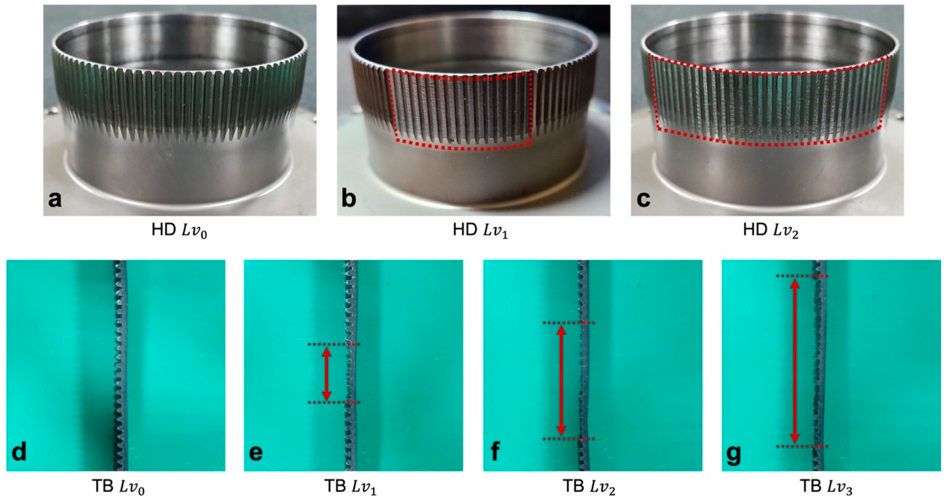
Artificial faults are introduced on both the HD and TB by removing a portion of teeth to simulate wear, as shown in Figure 6. In the subsequent sections, denotes the fault label, where is normal, and 1~3 are faults of different severities. In the HD, faults are introduced by cutting away the upper half of the teeth of the main gear, which is also called the flex spline and has 100 teeth, as shown in the upper figure. Two severities are considered: an fault is introduced to 1/6 of the teeth, and an fault to 1/3, which is double the number of the fault. Figure 6a–c illustrate examples of the change from normal to in terms of faulty teeth of the HD, where faulty teeth areas are marked with a red square. In the case of the TB, only a part of the teeth, of which there are 21, is meshed with the pulley when traveling back and forth in operation. Due to this, faults of the TB are created on these teeth. Similar to the HD, the upper half of the teeth is removed to introduce the fault. Three severities are considered: and faults are introduced to 7 and 14 teeth, respectively. faults are made to all 21 teeth. Figure 6d–g are the examples of normal and faulty teeth of TB, respectively.
As a result, the HD and TB undergo three and four different health conditions, respectively. Experiments are conducted for all the combinations of these conditions, resulting in a total of 12 experiments. In the case of the most severe fault (HD and TB ), however, the robot encounters failure by reporting the PID error message. Therefore, the data are available for only 11 experiments.
3.2. Data Acquisition
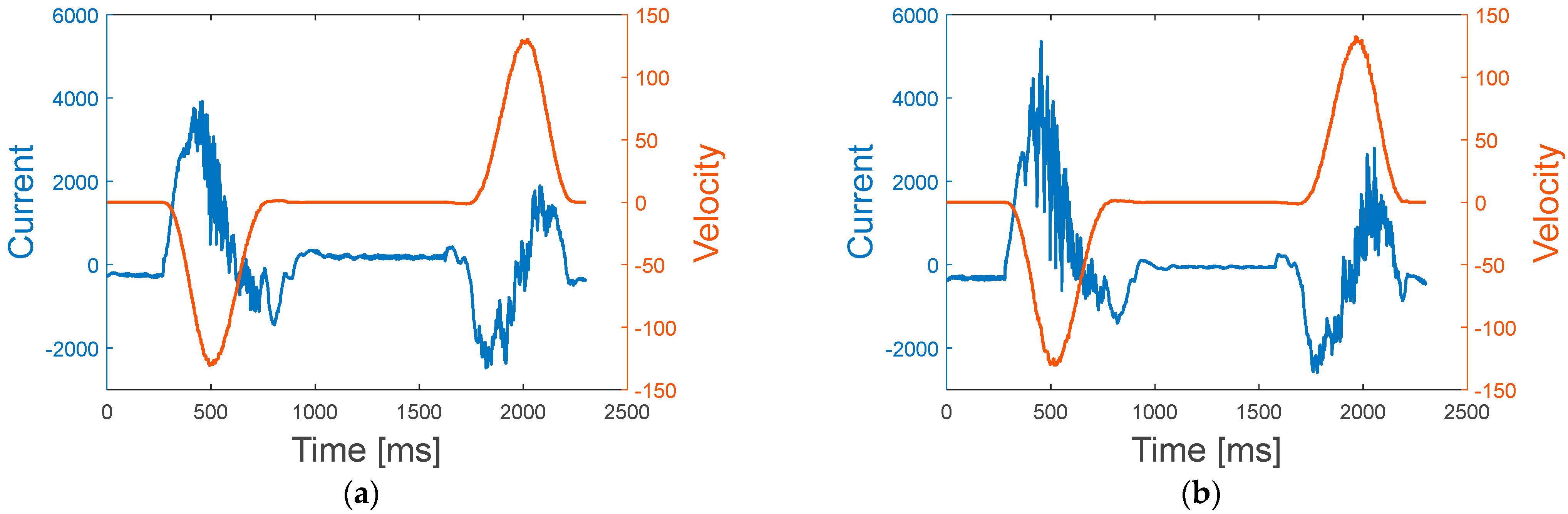
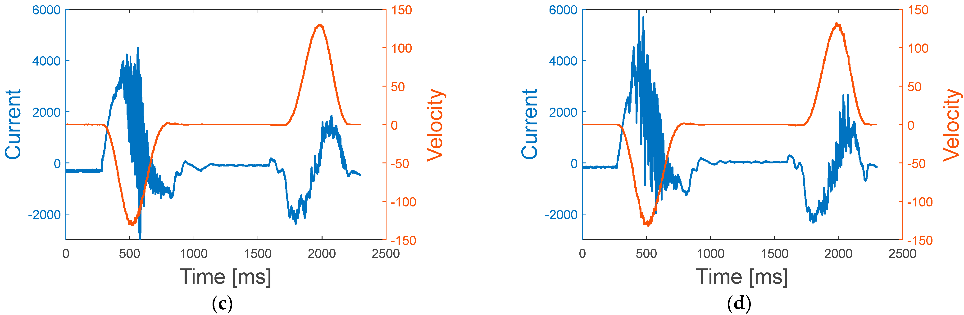
Among the several operational scenarios for the robot, the simplest case is considered in this study, which consists of performing a wafer pick motion to a certain LPM and returning. The robot repeats this operation for 24 to 25 cycles per minute. Operation commands are input by the control panel, which is transmitted to the robot by the controller. During the operation, the current and velocity of the motor, and the control signal GPL indicating operation status, are acquired with 1 kHz from the controller by the laptop computer. Vibration in the vertical direction is also measured with 25.6 kHz by an attached accelerometer at the end-effector, as shown in Figure 5a, to assess the system performance. Motor signals are collected for 100 repeated cycles in a single experimental condition which lasts about 60 s. Unlike the control signal, in the case of the vibration, the signals are collected only five times due to a synchronizing problem with the motor control signal. Since this is a preliminary study for multi-component fault diagnosis, there are limitations that are different to the field conditions. First, the study is conducted for a simple operation, while the robot performs more complex operations in the field. Second, the control signal is collected at a sampling rate of 1 kHz, whereas it is 50 Hz in the field. The reason is that the robot company uses a higher sampling rate of 1 kHz when they test their robot performance in the lab, and this was the same in our study. As mentioned in the conclusion, these may be the challenges that should be incorporated when assessing practical applications, and are left as future work. The raw motor signals for the four fault conditions are shown in Figure 7, in which Figure 7a represents the fault conditions when all components are normal, Figure 7b represents the HD at , Figure 7c represents the TB at , and Figure 7d represents both the HD and TB at fault conditions. The figure representing the motor controls the movement so that the end effector moves a distance to one side, stays for a moment, and returns to the original position. In the current signal, it is observed that the fluctuations of the faulty conditions represented in Figure 7b–d are relatively high in the periods of 400–900 and 1700–2200 msec as compared with the normal Figure 7a. This occurrence in the current signal is to compensate for the faults in order to maintain the velocity profile in operation. The objective of this study is to investigate this difference and diagnose the health conditions of each component and the system by means of the proposed method.
4. Case Study
In this section, the proposed method is applied to and validated for axis 3 of the robot using the acquired signal from the motor with designed experiments. First, we discuss the feature extraction results for various fault conditions and the feature selection for model construction. Then, the performance of the diagnosis model for the components’ health and system performance is evaluated. Finally, the interactions between faulty components and their effect on the system performance are investigated.
4.1. Feature Extraction from Motor Control Signal
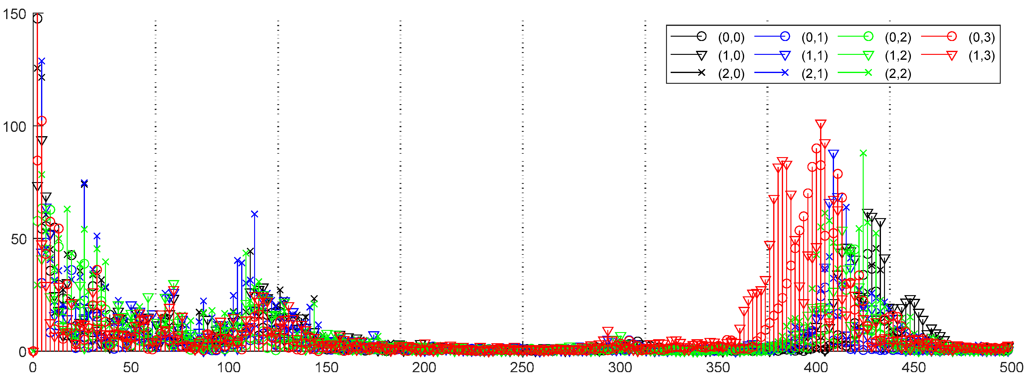
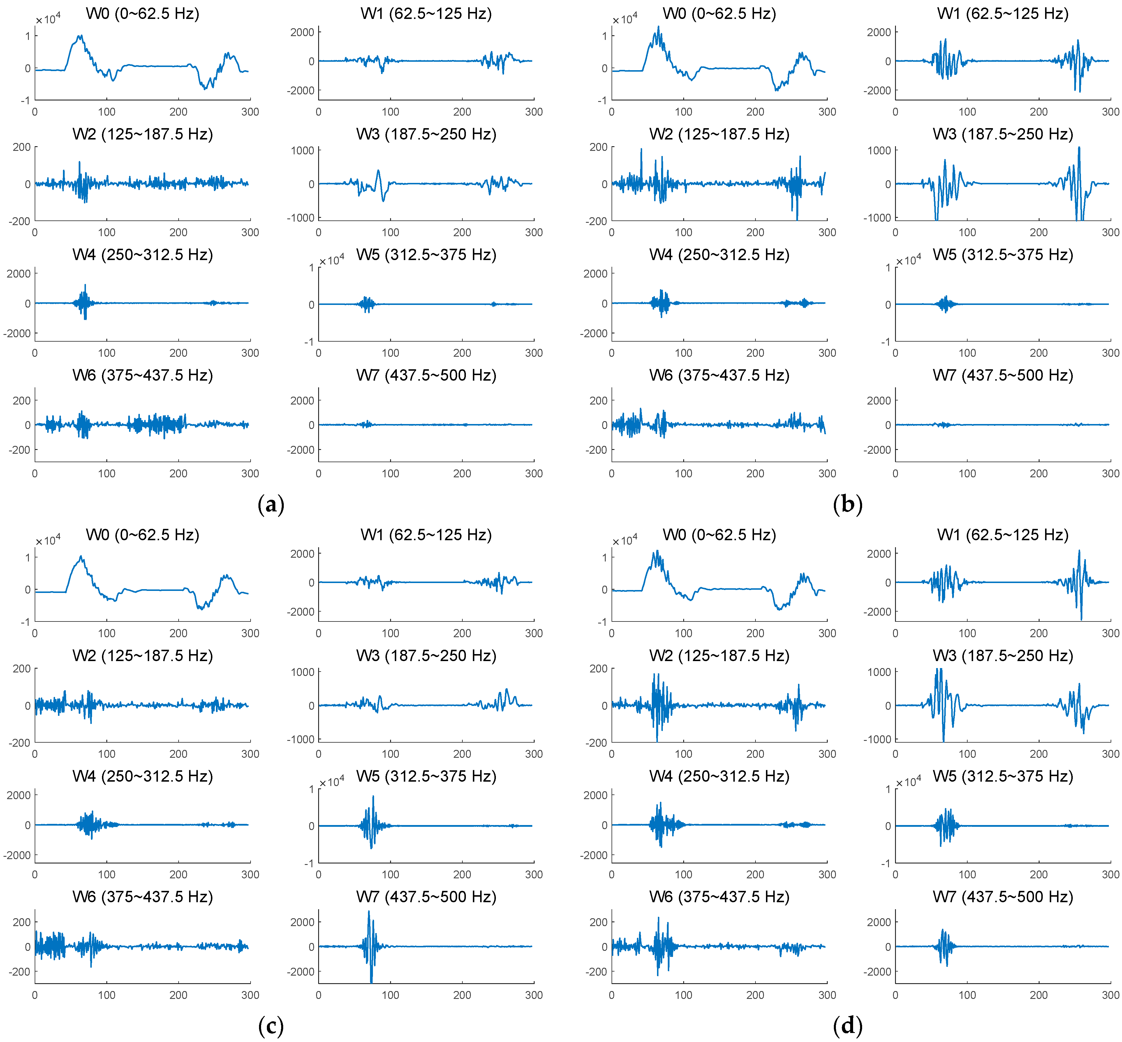
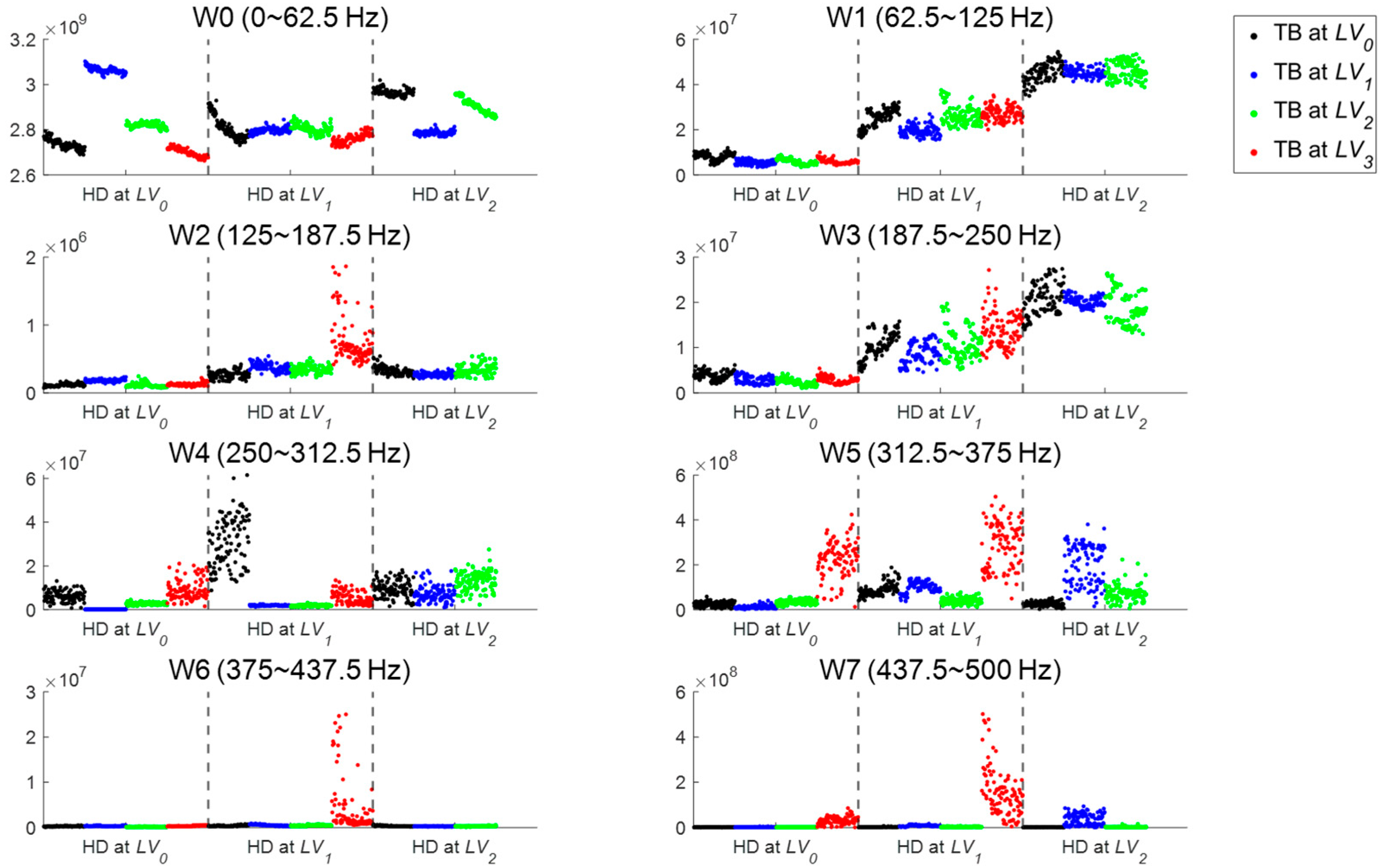
In order to extract good features representing faults in the motor control signal in operation, WPD is conducted to the current and velocity signal, in which Daubechies 6 (db6) and three levels are taken for the wavelet function and decomposition, respectively. These selections are based on similar studies by [28,29], in which the WPD and the Daubechies mother wavelet family are used to detect faults in an AC motor or components connected to the motor using the motor current signal. Since our aim is the same, namely, the fault diagnosis of components connected to the AC motor, the Daubechies family is employed. Regarding the level of decomposition, it is generally selected to adequately capture the fault characteristics in the frequency domain of the fault signals. To this end, the FFTs are performed to all the fault conditions of different severities, and the results are given in Figure 8, which shows each spectrum in superposition. The legend of the figure represents HD and TB . In this figure, differences are captured in specific frequency bands depending on the fault. Based on this observation, it follows that the three levels, namely, the eight bands (W0 to W7) with the length of 62.5 Hz, are enough to identify the difference between each fault condition. The bands are divided by the black dotted lines in the figure. The wavelet coefficients in each band for the four conditions are shown for the current signal in Figure 9, which exhibits a clear difference between the HD and TB faults: comparing the HD fault in Figure 9b to the normal in Figure 9a, the coefficient increases in the low-frequency bands W1, W2, and W3. On the other hand, in the TB fault in Figure 9c, the coefficient increases in the high-frequency bands W5, W6, and W7. In both the HD and TB with faults in Figure 9d, the coefficients increase in both the low- and high-frequency bands. In order to make a more quantitative comparison, wavelet energy (WE) is calculated by using Equation (4) using the coefficients at each frequency band, which are repeated for all the fault conditions. The results are plotted in Figure 10, where black, blue, green, and red dots indicate , , , and in TB faults, respectively, whereas HD faults are divided by vertical dotted lines. A similar observation is found, which is that the WE increases in the low-frequency bands W1 and W3 when the HD fault level increases. In the case of the TB, the WE increases in the high-frequency bands W5, 6, and 7 as the TB fault increases from to , although the increase is significant only at .
In addition to the WE, 13 statistical time-domain features commonly used in the fault diagnosis, as shown in Table 1 [19], are extracted for each of the eight frequency bands of the current signal. Applying the same process to the velocity signal, a total number of features are obtained for a single operation condition. The score as defined in Equation (11) is calculated for the 224 features, which accounts for the two metrics: for a consistent trend with respect to the fault severity and for the separability of each fault. After a parametric study to determine the weight parameter , the value 0.8 is found to be the most appropriate to meet both requirements. Since the calculation is performed for the components HD and TB, respectively, 224 scores are available for the features of each component. Note that the values are normalized so that they vary between 0 and 1.
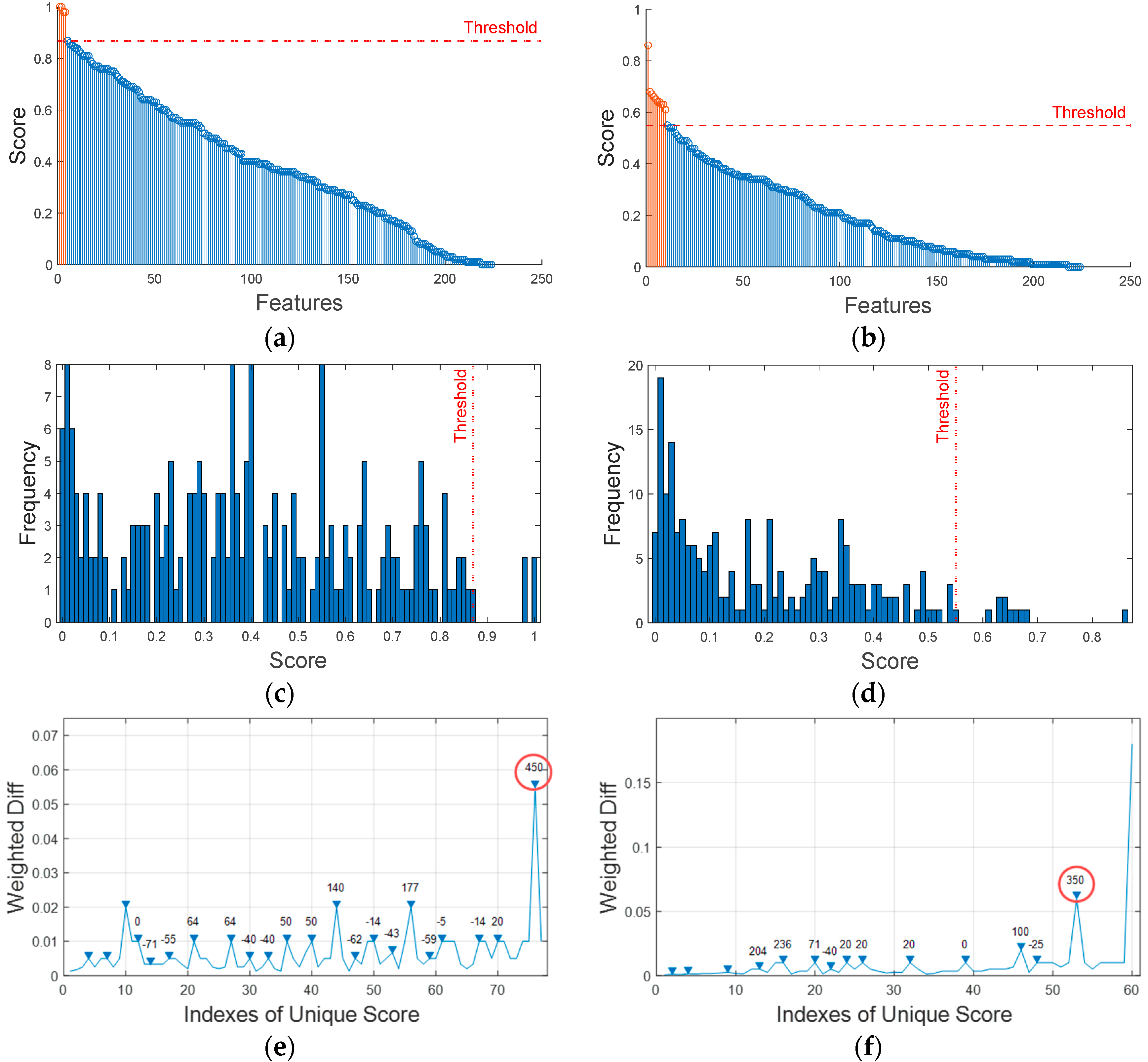
For these sets of scores, the RPN formula as described in Section 2.2 is applied to estimate the threshold and select the most significant features in a more logical manner. The resulting thresholds are shown in Figure 11a,b by the horizontal lines, which indicate the scores of all the features in descending order. The rest of the figures explain the process of estimating them. For example, in the case of the HD, the frequencies of the unique scores for all of the features are shown in Figure 11c. Using this information, the weighted finite differences defined by Equation (12) are computed, as shown by the curves in Figure 11e, from which the local peaks defined by Equation (14) are identified by the triangles and corresponding percent values. Among these, the index and its score, with a maximum of 450%, are found to be 76 and 0.87, which are marked with a red circle in Figure 11e and constitute the threshold in Figure 11a,c. Through this process, four features are selected for the HD, which are those higher than the threshold in Figure 11a.
In the final step, the redundancies between the selected features are checked by computing the Pearson correlation for a combination of pairs, in which those with a correlation higher than 0.9 are removed from the selection. As a result, the features are reduced to only one, which is W1-STD of the current signal, namely, the STD of the wavelet coefficient in the frequency band (62.5~125 Hz). The same process is applied to the TB to obtain Figure 11b,d,f, from which the features without redundancy are reduced to four features (W0-SF of the velocity, W7-MF, W7-Peak, and W7-SE of the current signal).
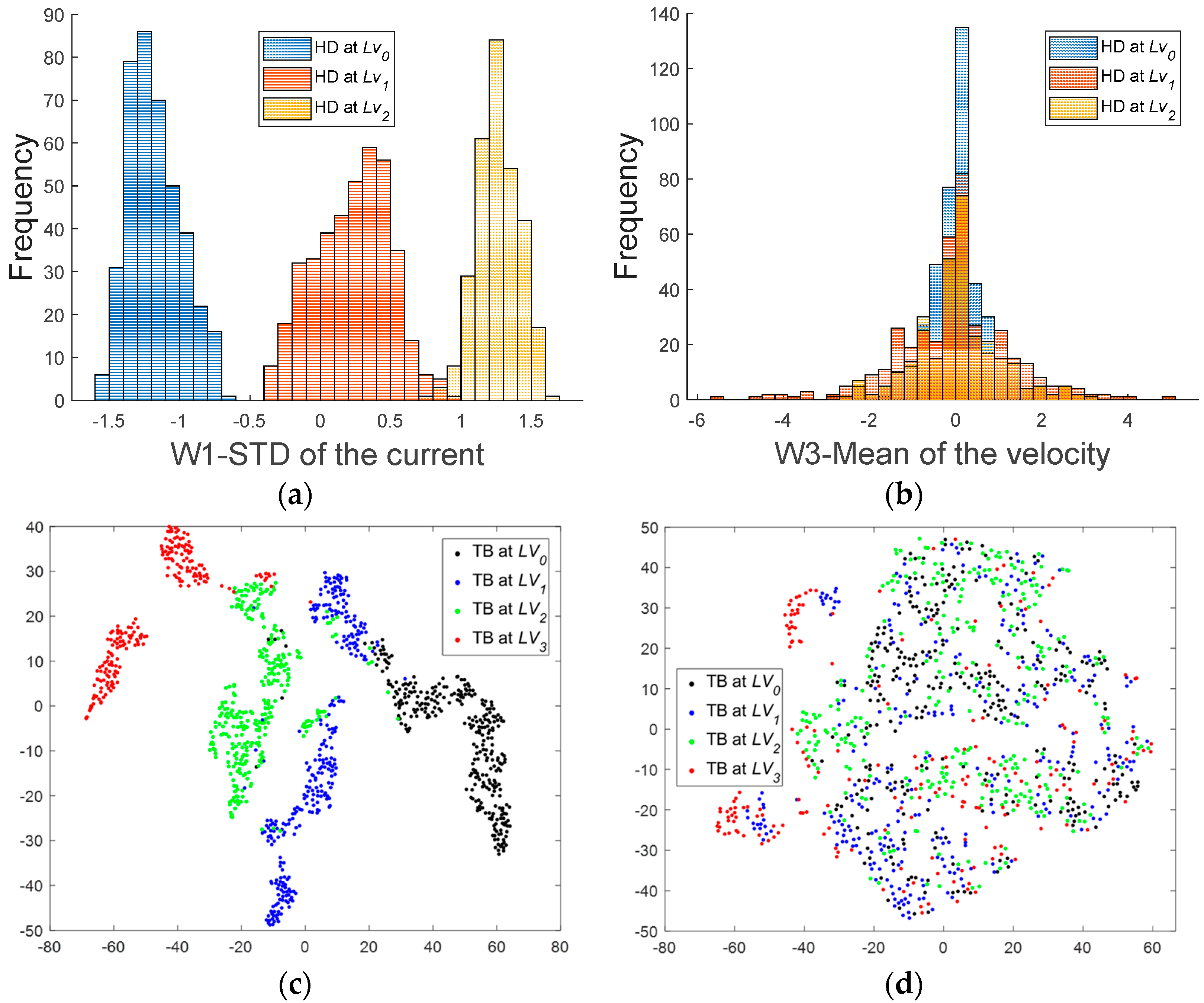
To illustrate the importance of the feature selection, plots of the best and worst features in view of the score are shown in Figure 12. In the case of the HD, the number of selected features is one, where the best is W1-STD of the current and the worst is W3-Mean of the velocity. Their histograms are shown in Figure 12a,b. In the case of the TB, the number of features is four, which are W0-SF of the velocity, W7-MF, W7-Peak, and W7-SE of the current. In this case, for the sake of visual comparison, t-distributed stochastic neighbor embedding (t-SNE) is used for the selected features, which is useful for visualizing the high-dimensional data by embedding the n-dimensional original feature space into the two-dimension [30]. The best four features are compared against the worst ones: W2-CF, W5-SK, W7-Mean, and W1-CF of the current signal, as shown in Figure 12c,d, respectively. The results of the HD and TB features all indicate that the selection of good features is important to the aspect of fault severity identification.
4.2. ANN Model Construction
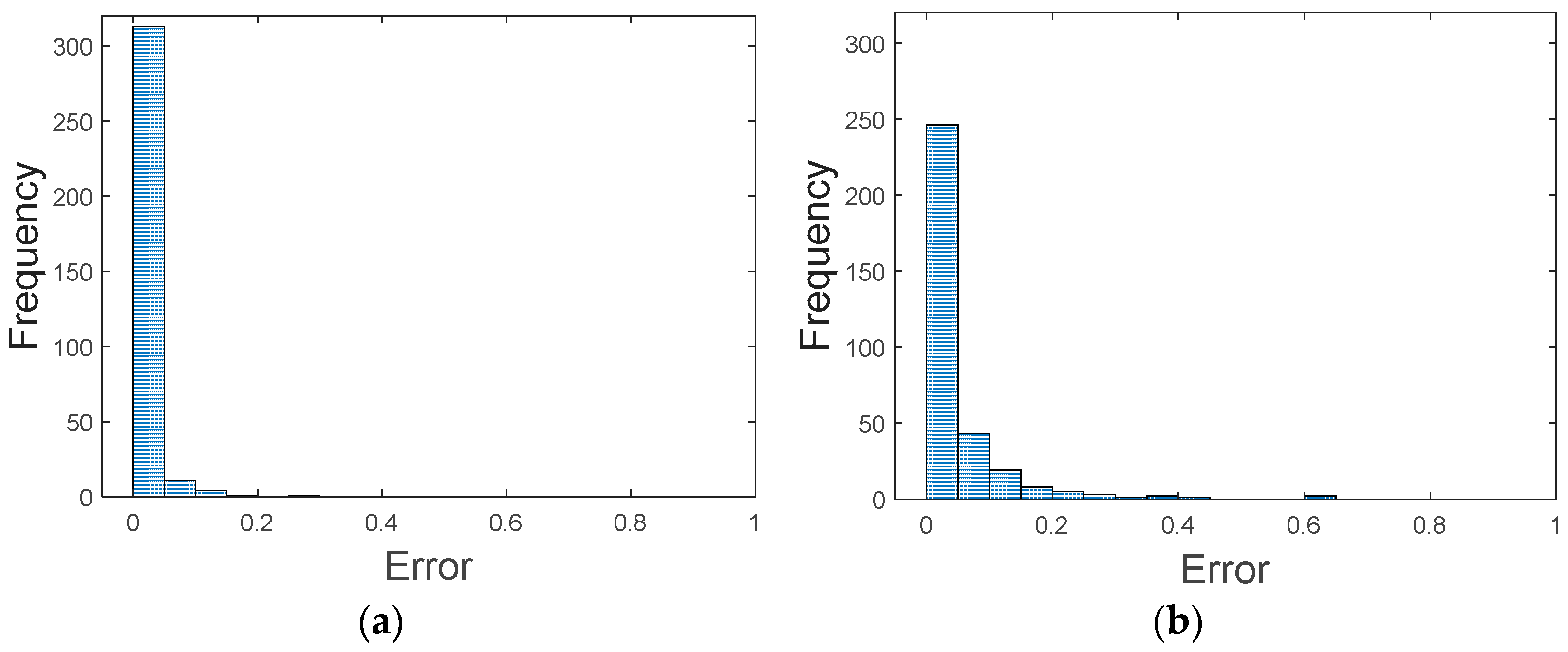
The five selected features (one for the HD and the others for the TB) from the previous section are used as the input nodes of the ANN, and the corresponding fault severities of the HD and TB as the output. Since there are 100 data points available for each of the 11 fault conditions, the total number of data points is . The model is trained using 70% of the datasets and the model accuracy is evaluated by the test datasets (30%). Note that in the model, the severity of each component is transformed into the health index (HI) so that it is 0 for the normal and 1 for the most severe condition. Hence, the HD fault levels of , , and correspond to 0, 0.5, and 1, and the TB fault levels of , , , and to 0, 1/3, 2/3, and 1. The structure of the ANN is given by a single hidden layer to avoid overfitting and reduce computational complexity. For the activation function, tan-sigmoid is selected. The number of nodes in the hidden layer is optimized through 5-fold cross-validation. For this purpose, the training datasets are further divided into training and validation sets by a ratio of 4 to 1. The ANN model is trained with the training set while the accuracy is calculated using the validation sets. The process is repeated five times by choosing the sets at a ratio of 4 to 1 at random, from which the average accuracy is obtained for each hyper-parameter. As a result, the model showing the highest accuracy is chosen among the number of nodes from 1 to 50, which is 22. Finally, the ANN is trained using the training datasets with the optimized parameter and applied to the test dataset to predict the HI of each data. The histograms of the error between the predicted (output) and true (target) HI for the 330 test data sets are given in Figure 13 for the HD and TB, respectively. The root mean square error (RMSE) of these are also calculated, and are 0.0275 and 0.0902.
4.3. GPR Model Construction
As addressed above, the robot system performance is defined by the root mean square (RMS) of the vibration in the z-direction at the end-effector axis. This is measured during robot operation under conditions of various faults of different severities for the HD and TB. Before construction of the GPR model, it is desirable to investigate the relative importance of each component in the system performance, including their interaction effect. For this purpose, analysis of variance (ANOVA) is performed, in which input factors with a -value smaller than 0.05 are regarded as statistically significant. The results are given in Table 2, which states that all three factors, namely, the HD, TB, and their interaction, affect the system performance significantly. While the most significant is the HD, as shown in the F-value, it should be noted that the result should be interpreted as a result of the wider severity range that was imposed by the authors. If the severity is reduced, the value will decrease accordingly. Another note is that the influence of the TB and its interaction with the HD are similar in magnitude, which indicates that their interaction clearly exists and should be incorporated into the system model.
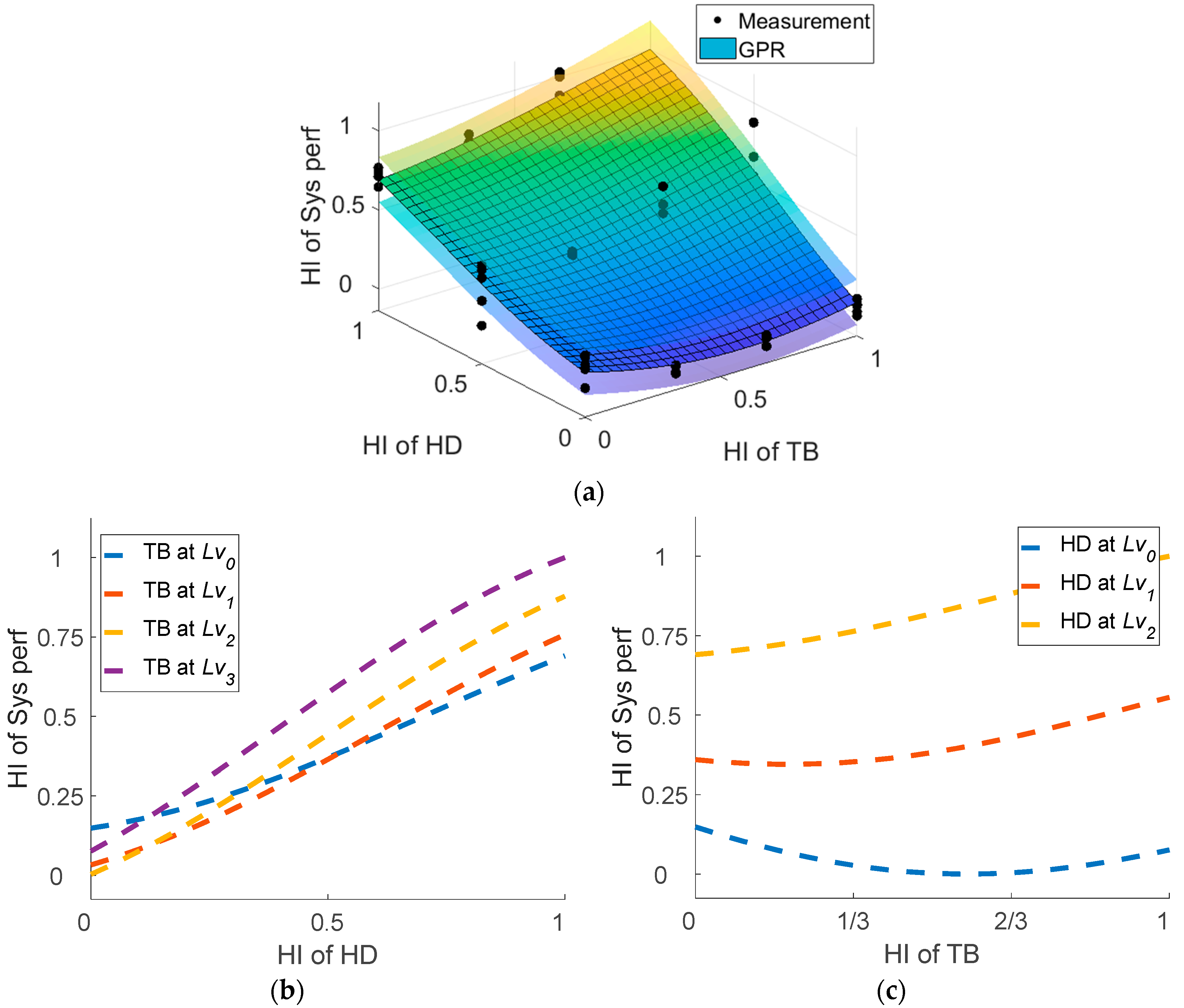
Based on this understanding, a GPR model for the system performance is constructed, which is able to capture the interactive relation, with the input as the HI of the HD and TB, and the output as the RMS of the vibration. In the model, as for the components, the predicted RMS values are normalized into the HI with a range [0, 1] as the system performance. The hyper-parameters are optimized at 0.9525, 0.0467, and 0.0130 with the training datasets by maximizing the marginal log-likelihood of the GPR. The result is given by the response surface plot along with the confidence bounds, as shown in Figure 14a, in which the five black dots at each fault condition indicate the HI values from the RMS of measured vibration, and the confidence bounds are given by the shaded surface. The trend of the RMS in terms of the respective HD and TB axes reveals that the HD affects the system performance much more than the TB, but this is as a result of a wider severity range for the HD. The nonplanar shape of the response surface indicates that the HD and TB affect the system performance interactively. Figure 14b,c are the mean responses as a function of the HD and TB severities while the other is fixed, respectively.
4.4. Application of the Models
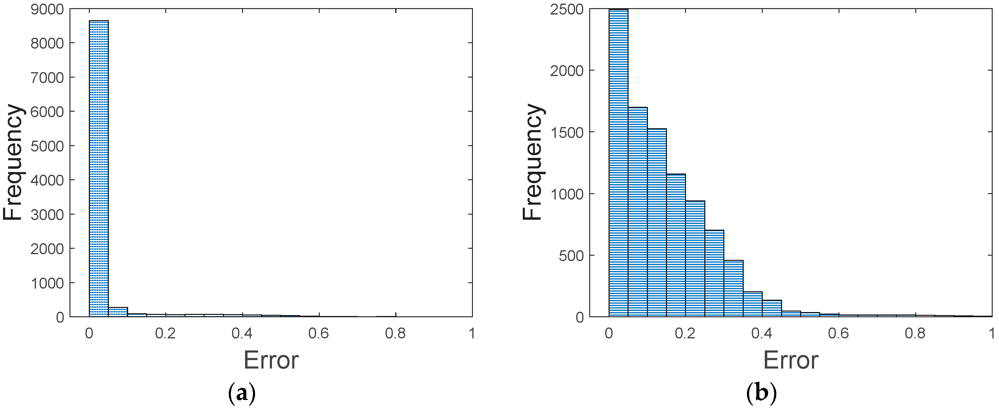
Once the two models are made available through the previous steps, they are applied to diagnose the state of health of a new robot in operation. However, the data acquisition for a new robot is not an easy task, but requires additional effort and time in order to create an artificial fault at another severity level. Therefore, in this study, more emphasis is given to explaining how the developed methodology can be applied by introducing a virtual measurement, developed by interpolating the features between the existing training data. Although the ANN and GPR models are nonlinear by nature with respect to the fault severities of the HD and TB, the target (true) HIs are also assumed by the interpolation of the training data ignoring the nonlinearity. In order to examine how much error will be introduced by this approach, virtual data are generated only for the 11 existing fault conditions by interpolation. For example, a new condition (HD at , TB at ), which is also present in the existing conditions, can be generated by interpolating the two conditions HD at , TB at and HD at , TB at . These are considered in the evaluation. However, conditions such as the interpolation of HD at , TB at and HD at , TB at are avoided since they are not in the existing conditions. After investigation, the 11 new conditions are obtained, as shown in Table 3. Recall that there are 30 data points (30% of the whole dataset) for each fault condition in the test dataset. Then, one can construct new virtual features by interpolation, which amounts to a total of data points. The trained ANN model is then applied to these data to predict the state of health of each component and calculate the error between the output and target HI. The resulting histograms for the errors of the 9900 data points are given in Figure 15. Comparing with Figure 13, it is found that the RMSEs are 0.091 and 0.195, which are greater by 3.3 and 2.2 times, for the HD and TB, respectively. However, the authors believe that these are acceptable for estimating the HI in the dimension of [0, 1], which is because of the somewhat lower degree of nonlinearity.
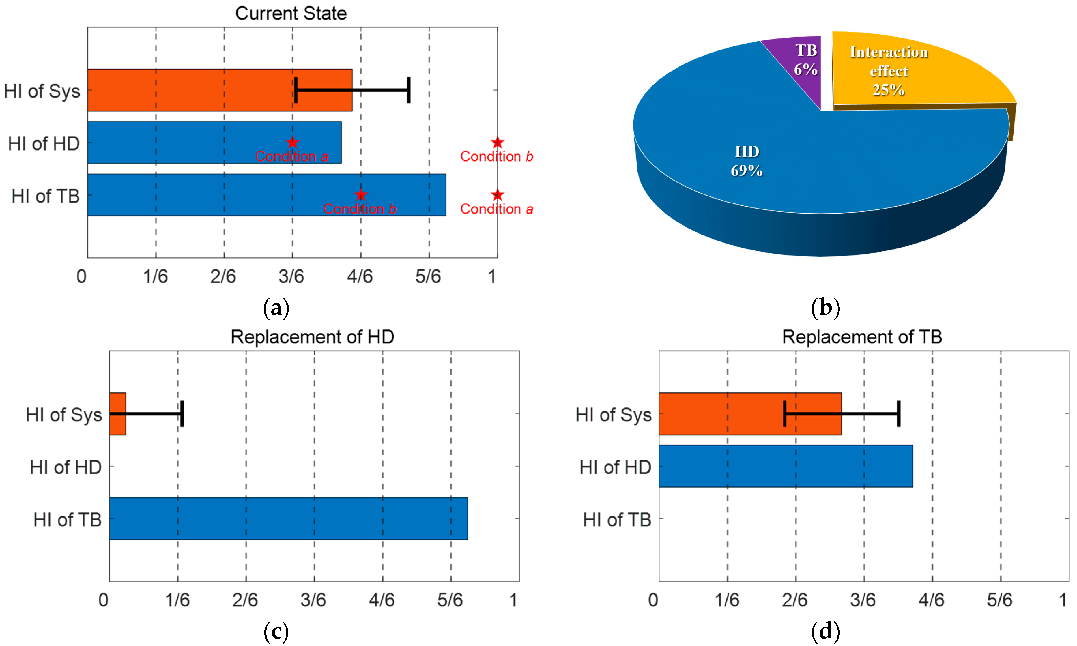
With this understanding, let us now apply the model to a new case, in which the robot is operated in a condition halfway between the two existing conditions denoted by (HD at 0.5, TB at 1) and (HD at 1, TB at 2/3) in the HI. Then we will expect that the HIs of the HD and TB will be somewhere around the interpolated ones, that is, 0.75 and 0.83 respectively. Assume that the motor control signal is acquired under this condition, from which the five feature values are obtained by the signal processing as mentioned in Section 4.1, although these are in fact obtained by interpolating the values of conditions and . Applying these to the ANN model, the HIs of each component are obtained as 0.62 and 0.87 for the HD and TB, respectively. Then, apply these to the GPR model to obtain the HI of system performance, which is 0.65 with the confidence bounds [0.51, 0.78]. This is summarized in Figure 16a in the form of a bar chart, in which the error bar indicates the confidence interval.
Once we have the GPR model, the advantage is that we can perform what-if analysis: how well the system performance will be restored when a component is replaced by a new one. This is performed by changing the HI of the component to 0 in the model. The resulting HIs are 0.04 and 0.45, as shown in Figure 16c,d, for HD and TB, respectively. Comparing the two HIs, in view of the maintenance strategy, Figure 16c in which the HD is replaced is advised, since it restores the system performance more fully. Figure 16b shows the contribution ratio of the HD, TB, and their interaction effect on the system health degradation, in which the areas by the HD and TB are given by the restored HI by replacing each component. For the HD and TB, the HIs are restored from 0.65 to 0.04 and 0.45, hence, the restored HIs are 0.61 and 0.20, respectively. Note, however, that the sum of these two is 0.49, which does not agree with the HI of the current system due to the interaction effect, which is 0.16. By normalization, these values are transferred into the ratio, as shown in the figure. Based on this information, the equipment engineer can diagnose the current health of the system and make appropriate decisions in terms of which component to replace early, before failure. Although this is illustrated via virtual data, the procedure is the same when the signals are acquired in the real operation of a new robot: At first, using the motor control signal, extract five significant feature values. Second, apply the five feature values to the ANN model to estimate the fault severities of the two components, the HD and the TB. Third, apply the two severity values to the GPR model to estimate the current system performance, which will look like the performance illustrated in Figure 16a. Finally, perform the what-if analysis as in Figure 16c,d by restoring the health of either component and make maintenance decisions based on the results.
5. Conclusions and Future Work
It is crucial to diagnose the condition of industrial robots to prevent losses caused by downtime in manufacturing plants. In this paper, we proposed a methodology to conduct a system-level diagnosis for wafer transfer robots that consists of two critical components (harmonic drive and timing belt), the degradation of which leads to the failure of the system, characterized by end-effector vibration. The procedure is summarized as follows: First, informative features are extracted from the motor control signal through signal processing techniques which apply the WPD for feature extraction and the RPN formula of hybrid score for feature selection. Second, an ANN is established to model the relation between extracted features and the HI of components. The model achieves RMS errors of 0.0275 and 0.0902 for the HD and TB, for the HI in the range of 0 to 1. Third, GPR is applied to build the relationship between HIs of components and the system. Before construction, it is found that the interaction between the two components, the HD and TB, is significant: the F-value 5.38 in ANOVA for the interaction is similar in magnitude to 4.09 for the TB. Finally, the ANN and GPR models are applied to the new robot in operation, in which the current state of health of the two components, as well as the system performance, are estimated, and a maintenance strategy is determined by evaluating how well the system performance is restored by the replacement of each component. Using the example mentioned in Section 4.4 as an illustration, the HIs of the two components and the system are 0.62, 0.87, and 0.65. After the replacement of each component to a new one, the system HI is restored to 0.04 and 0.45, respectively, which indicates that replacing the HD leads to three times better system health.
The contributions of the proposed methodology can be stated as follows: First, the authors have examined multiple components and their fault severities, which can account for the interaction relationship in degradation between the components and system. Second, motor control signals are exploited, which are acquired automatically during operation with no additional use of sensors. Third, a hybrid score and an RPN-based formula are applied to select the most appropriate features for the diagnosis in a more objective way. Last, but not least, a system-level approach is proposed, which evaluates the state of health of the components, conditional on the system performance, as opposed to the traditional component-level approach. Thanks to this, a proper maintenance policy can be developed to decide which component to replace and how well the system health is restored.
However, several critical challenges remain in the implementation of this study: First, the model development requires costly and time-consuming experiments for fault seeding and operation for a variety of degradation conditions. In this study, only two components with three or four severity levels are considered, which have operated under 12 different conditions. The number of cases will increase exponentially for more components and severity levels, which requires an efficient strategy for the design of experiments. Second, in the fault seeding process, a good domain knowledge is critical, which includes the type of failure modes, ways of fault seeding, and the degree of degradation. Unless this is properly addressed, the result will be significantly different from those in the field, and hence, will be useless. In this study, the artificial faults are based on the literature on robot faults, which have, however, been empirical or intuitive. Third, the proposed model is developed based on a specific operation profile such as a simple round trip of a wafer at a certain speed. If the profile changes or becomes more complex, the resulting features and subsequent ANN and GPR models will be changed accordingly. Since we cannot do this every time the profile changes, a more general strategy is needed to address this issue. Lastly, there is a difference in the sampling rate in the data acquisition of the motor signal between our study and the field, which are 1 kHz and 50 Hz, respectively. Due to issues with data storage and handling, lower sampling rates are used in the field. In this case, a different strategy should be developed, because the frequency band and resolution may be different. Future studies will be performed to overcome these challenges. Towards this objective, we plan to generalize our methodology for a few different operation profiles with lower sampling rates used in the field, and validate its performance.
Author Contributions
Conceptualization, J.-H.C. and H.J.P.; methodology, I.L.; software, H.J.P.; validation, I.L. and H.J.P.; formal analysis, I.L.; investigation, H.J.P. and I.L.; resources, C.-W.K.; data curation, J.-W.J.; writing—original draft preparation, I.L. and H.J.P.; writing—review and editing, J.-H.C.; supervision, J.-H.C.; project administration, J.-H.C.; I.L. and H.J.P. contributed equally to this work and should be considered co-first authors. All authors have read and agreed to the published version of the manuscript.
Funding
This research was supported by Korea Electric Power Corporation. (Grant number: R22XO02-01).
Institutional Review Board Statement
Not applicable.
Informed Consent Statement
Not applicable.
Data Availability Statement
Not applicable.
Conflicts of Interest
The authors declare no conflict of interest.
References
- Kim, Y.; Park, J.; Na, K.; Yuan, H.; Youn, B.D.; Kang, C. Soon Phase-Based Time Domain Averaging (PTDA) for Fault Detection of a Gearbox in an Industrial Robot Using Vibration Signals. Mech. Syst. Signal Process. 2020, 138, 106544. [Google Scholar] [CrossRef]
- Capisani, L.M.; Ferrara, A.; Ferreira, A.; Fridman, L. Higher Order Sliding Mode Observers for Actuator Faults Diagnosis in Robot Manipulators. In Proceedings of the IEEE International Symposium on Industrial Electronics, Bari, Italy, 4–7 July 2010; pp. 2103–2108. [Google Scholar]
- Yang, Q.; Li, X.; Wang, Y.; Ainapure, A.; Lee, J. Fault Diagnosis of Ball Screw in Industrial Robots Using Non-Stationary Motor Current Signals; Elsevier: Amsterdam, The Netherlands, 2020; Volume 48, pp. 1102–1108. [Google Scholar]
- Cheng, F.; Raghavan, A.; Jung, D.; Sasaki, Y.; Tajika, Y. High-Accuracy Unsupervised Fault Detection of Industrial Robots Using Current Signal Analysis. In Proceedings of the 2019 IEEE International Conference on Prognostics and Health Management (ICPHM), San Francisco, CA, USA, 17–20 June 2019; ISBN 9781538683576. [Google Scholar]
- Chen, T.; Liu, X.; Xia, B.; Wang, W.; Lai, Y. Unsupervised Anomaly Detection of Industrial Robots Using Sliding-Window Convolutional Variational Autoencoder. IEEE Access 2020, 8, 47072–47081. [Google Scholar] [CrossRef]
- Jaber, A.A.; Bicker, R. Industrial Robot Backlash Fault Diagnosis Based on Discrete Wavelet Transform and Artificial Neural Network. J. Math. Sci. Appl. 2016, 4, 21–31. [Google Scholar]
- Kim, H.; Lee, H.; Kim, S.W. Current Only-Based Fault Diagnosis Method for Industrial Robot Control Cables. Sensors 2022, 22, 1917. [Google Scholar] [CrossRef] [PubMed]
- Huh, J.; Van, H.P.; Han, S.; Choi, H.J.; Choi, S.K. A Data-Driven Approach for the Diagnosis of Mechanical Systems Using Trained Subtracted Signal Spectrograms. Sensors 2019, 19, 1055. [Google Scholar] [CrossRef] [PubMed]
- Guo, J.; Li, X.; Lao, Z.; Luo, Y.; Wu, J.; Zhang, S. Fault Diagnosis of Industrial Robot Reducer by an Extreme Learning Machine with a Level-Based Learning Swarm Optimizer. Adv. Mech. Eng. 2021, 13, 16878140211019540. [Google Scholar] [CrossRef]
- Chen, L.; Cao, J.; Wu, K.; Zhang, Z. Application of Generalized Frequency Response Functions and Improved Convolutional Neural Network to Fault Diagnosis of Heavy-Duty Industrial Robot. Robot. Comput. Integr. Manuf. 2022, 73, 102228. [Google Scholar] [CrossRef]
- Long, J.; Mou, J.; Zhang, L.; Zhang, S.; Li, C. Attitude Data-Based Deep Hybrid Learning Architecture for Intelligent Fault Diagnosis of Multi-Joint Industrial Robots. J. Manuf. Syst. 2021, 61, 736–745. [Google Scholar] [CrossRef]
- Rohan, A.; Raouf, I.; Kim, H.S. Rotate Vector (Rv) Reducer Fault Detection and Diagnosis System: Towards Component Level Prognostics and Health Management (Phm). Sensors 2020, 20, 6845. [Google Scholar] [CrossRef]
- Kibira, D.; Shao, G.; Weiss, B.A. Buiding a Digital Twin for Robot Workcell Prognostics and Health Management. In Proceedings of the 2021 Winter Simulation Conference (WSC), Phoenix, AZ, USA, 12–15 December 2021. [Google Scholar] [CrossRef]
- Qin, C.; Jin, Y.; Zhang, Z.; Yu, H.; Tao, J.; Sun, H.; Liu, C. Anti-Noise Diesel Engine Misfire Diagnosis Using a Multi-Scale CNN-LSTM Neural Network with Denoising Module. CAAI Trans. Intell. Technol. 2023, 1–24. [Google Scholar] [CrossRef]
- Hsu, H.K.; Ting, H.Y.; Huang, M.B.; Huang, H.P. Intelligent Fault Detection, Diagnosis and Health Evaluation for Industrial Robots. Mechanika 2021, 27, 70–79. [Google Scholar] [CrossRef]
- Zhao, L.Y.; Wang, L.; Yan, R.Q. Rolling Bearing Fault Diagnosis Based on Wavelet Packet Decomposition and Multi-Scale Permutation Entropy. Entropy 2015, 17, 6447–6461. [Google Scholar] [CrossRef]
- Feng, H.; Chen, R.; Wang, Y. Feature Extraction for Fault Diagnosis Based on Wavelet Packet Decomposition: An Application on Linear Rolling Guide. Adv. Mech. Eng. 2018, 10, 1687814018796367. [Google Scholar] [CrossRef]
- Sim, J.; Kim, S.; Park, H.J.; Choi, J.H. A Tutorial for Feature Engineering in the Prognostics and Health Management of Gears and Bearings. Appl. Sci. 2020, 10, 5639. [Google Scholar] [CrossRef]
- Yan, X.; Jia, M. A Novel Optimized SVM Classification Algorithm with Multi-Domain Feature and Its Application to Fault Diagnosis of Rolling Bearing. Neurocomputing 2018, 313, 47–64. [Google Scholar] [CrossRef]
- Rajeswari, C.; Sathiyabhama, B.; Devendiran, S.; Manivannan, K. Bearing Fault Diagnosis Using Wavelet Packet Transform, Hybrid PSO and Support Vector Machine. Procedia Eng. 2014, 97, 1772–1783. [Google Scholar] [CrossRef]
- Catelani, M.; Ciani, L.; Galar, D.; Guidi, G.; Matucci, S.; Patrizi, G. FMECA Assessment for Railway Safety-Critical Systems Investigating a New Risk Threshold Method. IEEE Access 2021, 9, 86243–86253. [Google Scholar] [CrossRef]
- Kim, S.; Choi, J.H.; Kim, N.H. Challenges and Opportunities of System-Level Prognostics. Sensors 2021, 21, 7655. [Google Scholar] [CrossRef] [PubMed]
- Kim, S.; Choi, J.H.; Kim, N.H. Inspection Schedule for Prognostics with Uncertainty Management. Reliab. Eng. Syst. Saf. 2022, 222, 108391. [Google Scholar] [CrossRef]
- Liu, D.; Pang, J.; Zhou, J.; Peng, Y.; Pecht, M. Prognostics for State of Health Estimation of Lithium-Ion Batteries Based on Combination Gaussian Process Functional Regression. Microelectron. Reliab. 2013, 53, 832–839. [Google Scholar] [CrossRef]
- Zhou, D.; Yin, H.; Fu, P.; Song, X.; Lu, W.; Yuan, L.; Fu, Z. Prognostics for State of Health of Lithium-Ion Batteries Based on Gaussian Process Regression. Math. Probl. Eng. 2018, 2018, 8358025. [Google Scholar] [CrossRef]
- Pierleoni, P.; Belli, A.; Palma, L.; Sabbatini, L. Diagnosis and Prognosis of a Cartesian Robot’s Drive Belt Looseness. In Proceedings of the 2020 IEEE International Conference on Internet of Things and Intelligence System (IoTaIS), Bali, Indonesia, 27–28 January 2021; pp. 172–176. [Google Scholar] [CrossRef]
- Yang, G.; Zhong, Y.; Yang, L.; Du, R. Fault Detection of Harmonic Drive Using Multiscale Convolutional Neural Network. IEEE Trans. Instrum. Meas. 2021, 70, 3502411. [Google Scholar] [CrossRef]
- Cekic, Y.; Eren, L. Broken Rotor Bar Detection via Four-Band Wavelet Packet Decomposition of Motor Current. Electr. Eng. 2018, 100, 1957–1962. [Google Scholar] [CrossRef]
- Gan, C.; Wu, J.; Yang, S.; Hu, Y.; Cao, W. Wavelet Packet Decomposition-Based Fault Diagnosis Scheme for SRM Drives with a Single Current Sensor. IEEE Trans. Energy Convers. 2016, 31, 303–313. [Google Scholar] [CrossRef]
- van der Maaten, L.; Hinton, G. Visualizing Data Using T-SNE. Ann. Oper. Res. 2008, 620, 267–284. [Google Scholar] [CrossRef]
Figure 1.
System-level diagnosis framework: (a) diagnosis of component health; (b) estimation of system performance; (c) current state of health of components and system; (d) state of health after replacement of component A; and (e) state of health after replacement of component B.
Figure 1.
System-level diagnosis framework: (a) diagnosis of component health; (b) estimation of system performance; (c) current state of health of components and system; (d) state of health after replacement of component A; and (e) state of health after replacement of component B.

Figure 2.
Tree of wavelet packet decomposition.

Figure 3.
Features with different and : (a) case with low and high , (b) case with high and low , and (c) case with high and high ( in the figures indicates the fault severity level).
Figure 3.
Features with different and : (a) case with low and high , (b) case with high and low , and (c) case with high and high ( in the figures indicates the fault severity level).

Figure 4.
Schematic diagram of artificial neural network.

Figure 5.
(a) Wafer transfer robot and (b) target components of axis 3 in robot system.

Figure 6.
Artificially created wear damage on (a–c) harmonic drive (HD) and (d–g) timing belt (TB).

Figure 7.
Current and velocity signal under (a) normal conditions; (b) HD under conditions; (c) TB under conditions; and (d) both HD and TB under conditions.
Figure 7.
Current and velocity signal under (a) normal conditions; (b) HD under conditions; (c) TB under conditions; and (d) both HD and TB under conditions.


Figure 8.
Frequency spectrum for each of the 11 fault conditions.

Figure 9.
Wavelet coefficients of (a) normal condition; (b) HD at fault condition; (c) TB at fault condition; and (d) both HD and TB at fault condition.
Figure 9.
Wavelet coefficients of (a) normal condition; (b) HD at fault condition; (c) TB at fault condition; and (d) both HD and TB at fault condition.

Figure 10.
Wavelet energy of each decomposition band, where HD fault severities are divided by vertical dotted lines and TB fault severities are indicated by the color of the dots.
Figure 10.
Wavelet energy of each decomposition band, where HD fault severities are divided by vertical dotted lines and TB fault severities are indicated by the color of the dots.

Figure 11.
Threshold for (a) HD fault score and (b) TB fault score. Unique score frequency of (c) HD fault and (d) TB fault. Weighted difference of (e) HD fault score and (f) TB fault score.
Figure 11.
Threshold for (a) HD fault score and (b) TB fault score. Unique score frequency of (c) HD fault and (d) TB fault. Weighted difference of (e) HD fault score and (f) TB fault score.

Figure 12.
Histograms of (a) best feature and (b) worst feature for HD fault. t-SNE plots of (c) four best features and (d) four worst features for TB fault.
Figure 12.
Histograms of (a) best feature and (b) worst feature for HD fault. t-SNE plots of (c) four best features and (d) four worst features for TB fault.

Figure 13.
Error histogram for HI by ANN regression (a) for HD with RMSE 0.0275 and (b) for TB with RMSE 0.0902.
Figure 13.
Error histogram for HI by ANN regression (a) for HD with RMSE 0.0275 and (b) for TB with RMSE 0.0902.

Figure 14.
(a) Response surface plot of GPR with confidence interval; (b) responses in terms of HD fault with TB fault fixed; and (c) responses in terms of TB fault with HD fault fixed.
Figure 14.
(a) Response surface plot of GPR with confidence interval; (b) responses in terms of HD fault with TB fault fixed; and (c) responses in terms of TB fault with HD fault fixed.

Figure 15.
Error histogram for HI by ANN regression (a) for HD with RMSE 0.0911 and (b) for TB with RMSE 0.1955.
Figure 15.
Error histogram for HI by ANN regression (a) for HD with RMSE 0.0911 and (b) for TB with RMSE 0.1955.

Figure 16.
(a) Current state of health of components and system; (b) contribution of system performance degradation; (c) state of health after replacement of HD; and (d) state of health after replacement of TB.
Figure 16.
(a) Current state of health of components and system; (b) contribution of system performance degradation; (c) state of health after replacement of HD; and (d) state of health after replacement of TB.


Table 1.
Statistical features.
| Feature Name | Formula | Feature Name | Formula |
|---|---|---|---|
| Mean | Impulse factor (IF) | ||
| Standard deviation (STD) | Margin factor (MF) | ||
| Root mean square (RMS) | Peak | ||
| Skewness (SK) | Peak to peak (P2P) | ||
| Kurtosis (KUR) | Shannon entropy (SE) | ||
| Shape factor (SF) | Log energy entropy (LEE) | ||
| Crest factor (CF) |
Table 2.
ANOVA table.
| Source | Sum Sq. | d.f. | Mean Sq. | F | p-Value |
|---|---|---|---|---|---|
| TB | 0.0007 | 2 | 0.0003 | 4.09 | 0.0251 |
| HD | 0.0391 | 2 | 0.0196 | 233.6 | 0 |
| TB × HD | 0.0018 | 4 | 0.0005 | 5.38 | 0.0017 |
| Error | 0.0030 | 36 | 0.0001 | ||
| Total | 0.0446 | 44 |
Table 3.
New, but also present in the existing conditions, fault conditions are created by interpolating existing two conditions.
Table 3.
New, but also present in the existing conditions, fault conditions are created by interpolating existing two conditions.
| Virtual Data Fault Condition (HD , TB ) | Existing Fault Condition 1 (HD , TB ) | Existing Fault Condition 2 (HD , TB ) |
|---|---|---|
| (0, 1) | (0, 0) | (0, 2) |
| (1, 0) | (0, 0) | (2, 0) |
| (1, 1) | (0, 0) | (2, 2) |
| (0, 2) | (0, 1) | (0, 3) |
| (1, 1) | (0, 1) | (2, 1) |
| (1, 1) | (0, 2) | (2, 0) |
| (1, 2) | (0, 2) | (2, 2) |
| (1, 2) | (0, 3) | (2, 1) |
| (1, 1) | (1, 0) | (1, 2) |
| (1, 2) | (1, 1) | (1, 3) |
| (2, 1) | (2, 0) | (2, 2) |
Disclaimer/Publisher’s Note: The statements, opinions and data contained in all publications are solely those of the individual author(s) and contributor(s) and not of MDPI and/or the editor(s). MDPI and/or the editor(s) disclaim responsibility for any injury to people or property resulting from any ideas, methods, instructions or products referred to in the content. |
© 2023 by the authors. Licensee MDPI, Basel, Switzerland. This article is an open access article distributed under the terms and conditions of the Creative Commons Attribution (CC BY) license (https://creativecommons.org/licenses/by/4.0/).
Share and Cite
MDPI and ACS Style
Lee, I.; Park, H.J.; Jang, J.-W.; Kim, C.-W.; Choi, J.-H. System-Level Fault Diagnosis for an Industrial Wafer Transfer Robot with Multi-Component Failure Modes. Appl. Sci. 2023, 13, 10243. https://doi.org/10.3390/app131810243
AMA Style
Lee I, Park HJ, Jang J-W, Kim C-W, Choi J-H. System-Level Fault Diagnosis for an Industrial Wafer Transfer Robot with Multi-Component Failure Modes. Applied Sciences. 2023; 13(18):10243. https://doi.org/10.3390/app131810243
Chicago/Turabian StyleLee, Inu, Hyung Jun Park, Jae-Won Jang, Chang-Woo Kim, and Joo-Ho Choi. 2023. "System-Level Fault Diagnosis for an Industrial Wafer Transfer Robot with Multi-Component Failure Modes" Applied Sciences 13, no. 18: 10243. https://doi.org/10.3390/app131810243
Note that from the first issue of 2016, this journal uses article numbers instead of page numbers. See further details here.