Path Planning for Autonomous Vehicles in Unknown Dynamic Environment Based on Deep Reinforcement Learning

Abstract

Autonomous vehicles can reduce labor power during cargo transportation, and then improve transportation efficiency, for example, the automated guided vehicle (AGV) in the warehouse can improve the operation efficiency. To overcome the limitations of traditional path planning algorithms in unknown environments, such as reliance on high-precision maps, lack of generalization ability, and obstacle avoidance capability, this study focuses on investigating the Deep Q-Network and its derivative algorithm to enhance network and algorithm structures. A new algorithm named APF-D3QNPER is proposed, which combines the action output method of artificial potential field (APF) with the Dueling Double Deep Q Network algorithm, and experience sample rewards are considered in the experience playback portion of the traditional Deep Reinforcement Learning (DRL) algorithm, which enhances the convergence ability of the traditional DRL algorithm. A long short-term memory (LSTM) network is added to the state feature extraction network part to improve its adaptability in unknown environments and enhance its spatiotemporal sensitivity to the environment. The APF-D3QNPER algorithm is compared with mainstream deep reinforcement learning algorithms and traditional path planning algorithms using a robot operating system and the Gazebo simulation platform by conducting experiments. The results demonstrate that the APF-D3QNPER algorithm exhibits excellent generalization abilities in the simulation environment, and the convergence speed, the loss value, the path planning time, and the path planning length of the APF-D3QNPER algorithm are all less than for other algorithms in diverse scenarios.

1. Introduction

As autonomous driving technology advances, it significantly transforms the logistics industry. Autonomous vehicles eliminate the need for human drivers and utilize sensors and navigation systems to precisely plan and execute routes, enabling them to avoid congestion and traffic delays effectively. This enhances the overall efficiency of logistics operations. Moreover, autonomous driving technology enables real-time monitoring of vehicle location, status, and transportation processes, offering users more precise logistics information. This capability assists in optimizing transportation networks, enhancing supply chain efficiency, and providing decision-makers with a better basis for making informed decisions.

In 2012, Google conducted a test of its self-driving vehicle in Nevada, USA, covering a distance of 1.4 miles, which marked a significant milestone in the advancement of autonomous driving technology. In 2014, Tesla introduced the first generation of its self-driving system, known as Autopilot. In 2016, Google established Waymo, a company focused on developing commercial self-driving vehicles [1,2]. Subsequently, autonomous driving technology gradually made its way into the logistics industry. Amazon introduced its drone program called Prime Air to explore the feasibility of drone delivery. Companies, such as Nuro, Marble, Amazon (with its Scout autonomous logistics vehicle), and Einride (with its autonomous electric logistics vehicle in Sweden), entered the market and began regular operations in the autonomous logistics sector. In China, logistics platforms, such as Jingdong, Meituan, and Cainiao, have implemented autonomous vehicles for operational testing on university campuses and closed parks. Startups, such as New Stone and Wisdom Walker, have also ventured into the autonomous delivery field. Companies, such as Shunfeng and Jingdong, have been involved in the research and development of drones and have conducted trial operations. Suning’s electric autonomous vehicle, Wolong No. 1, is now in normal operation. Cainiao Logistics is actively conducting experiments related to autonomous urban logistics delivery. The application of autonomous driving technology in the logistics industry undoubtedly brings opportunities and challenges to the field.

Traditional path planning for autonomous vehicles can be categorized into local and global planning algorithms based on the scope of required environmental information [3]. Global path planning involves acquiring environmental information in advance and generating a map. The algorithm plans the path based on the starting and target poses on the map, as well as the positions of static and dynamic obstacles. Meanwhile, local path planning focuses on the immediate surroundings of the vehicle, utilizing sensor information to avoid static obstacles, predict the trajectory of sudden dynamic obstacles, and find feasible paths. In dynamic environments, autonomous vehicles often require global and local path planning. They use the global path as a general direction while dynamically avoiding obstacles and performing short-distance path planning with the assistance of local path planning [4]. Based on algorithmic principles, path planning methods can be classified into raster map-based, sampling-based, and bionic heuristic-based approaches [5,6,7,8,9,10,11]. Map-based methods include algorithms, such as Dijkstra’s algorithm, A*, and D*. Sampling-based methods encompass the RRT algorithm, PRM algorithm, and APF method. Bionic heuristic-based methods include genetic, particle swarm, neural network, and ant colony algorithms. However, existing path planning algorithms, such as A*, APF, and DWA still have certain limitations. The DWA algorithm, for instance, is only applicable to omnidirectional mobile autonomous vehicles as it requires the vehicle to perform in-place rotation for obstacle avoidance and path replanning. The APF algorithm faces challenges of unreachable targets and local minima. Meanwhile, the A* algorithm may result in unsmooth planning paths with excessive turns. The artificial potential field method is a path planning method with a simple principle, concise mathematical model, smooth path, and high computational efficiency and is commonly used in local obstacle avoidance movement. The artificial potential field method is favored because it requires less external information, a faster computation speed, and smoother planning paths, but there are problems such as insufficient planning ability in complex environments, and local minima and unreachable goals. Moreover, all three types of path planning algorithms rely on pre-established maps, which limits autonomous vehicles in exploring unknown environments.

The rapid development of deep learning, driven by the continuous advancements in computer hardware, has found extensive applications in various fields, including autonomous vehicles and computer vision. DRL, a combination of deep learning and reinforcement learning techniques, has gained significant attention [12]. In this approach, an intelligent agent interacts with an unknown environment (DRL), taking actions based on feedback from reward signals to achieve predefined goals [13]. The concept of reinforcement learning dates back to the early 20th century [14]. In 1992, Watkins introduced the Q-Learning algorithm, which marked a significant milestone in the development of reinforcement learning algorithms. The Q-Learning algorithm utilizes a Q-table to store the expected reward values for different actions in each state, enabling the agent to make optimal decisions in various states [15]. Rummery G and Niranjan further improved upon Q-Learning by introducing the Sarsa algorithm, an on-policy Q-Learning algorithm that performed better in learning control problems. However, as the complexity of the problems in terms of states and actions increases, maintaining a Q-table becomes increasingly challenging, leading to the problem of dimensional catastrophe. To address this issue, in 2013, Mnih et al. introduced the Deep Q-Network (DQN) algorithm, which combined the Q-Learning algorithm with convolutional neural networks. The DQN algorithm overcomes the problem of dimensional catastrophe by utilizing end-to-end mapping and simulating the Q-table model through neural networks. This breakthrough marked a new era in reinforcement learning [16]. In 2015, Nair A proposed the distributed DQN, which utilized a distributed approach to handle neural networks and experience replay buffers, thereby further improving learning efficiency [17].

Hasselt et al. introduced the Deep Double Q-Network (DDQN) to address the overestimation problem in the DQN algorithm. By utilizing two structurally identical networks, one for action selection and the other for Q-value estimation, the DDQN effectively mitigates the issue of overestimation that arises with single networks [18]. Wang et al. proposed an enhanced version of the DQN called Dueling DQN. This architecture incorporates a convolutional layer to extract input states, followed by a fully connected layer that splits the output into two parts: the value function and the action advantage function. This separation enables better learning of the value function [19]. To enhance the stability of the algorithm during training, Anschel et al. suggested calculating the average value of previously learned Q-values [20]. This approach reduces the variance of the approximation error, further improving algorithm stability. Dong Yongfeng et al. developed the DTDDQN network, which combined the Averaged-DQN and DoubleDQN algorithms while leveraging prior experience to reduce the discrepancy between estimated and true values [21]. Hausknecht et al. merged the DQN algorithm with LSTM networks, thereby allowing the LSTM network to learn and retain state information from moments before and after time t. This memory chain facilitates faster decision-making [22]. Schaul et al. proposed preferential empirical replay, where samples were selected from the replay pool based on their Time Difference error (TD-error) values as probabilities. This approach accelerates convergence [23]. Building upon priority experience replay, Liu Panfeng introduced an experience replay mechanism based on the entropy of state information to ensure sample diversity [24]. Bae et al. devised a multi-path planning algorithm for autonomous vehicles based on the DQN, enabling path planning in multiple environments [25]. Lei et al. applied the DQN algorithm to path planning, with the neural network taking environmental information acquired by the vehicle’s sensors as an input and outputting the state-action Q-value, achieving end-to-end mapping [26]. Lei et al. applied the Double DQN network to path planning in unknown environments. They continuously adjusted the target and starting positions during training to enhance the algorithm’s generalization ability in diverse location environments [27]. Tiong proposed the deep deterministic policy gradient (DDPG), a DRL algorithm for automatic driving simulation. DDPG models the path, following the control, reward function, actor-network, and critic network [28]. Du introduced the concept of maximum comfortable speed to represent the vertical ride comfort of roads. They designed a DRL algorithm to learn comfortable and energy-efficient speed control strategies [29]. Li et al. proposed a probabilistic model-based risk assessment method for evaluating driving risks using location uncertainty and distance-based safety indicators. They also developed a risk perception decision algorithm that utilized DRL to find strategies with the least expected risk. The proposed approach was evaluated using the CARLA simulator in two scenarios involving static obstacles and dynamically moving vehicles. The results demonstrate that the method can generate safe driving strategies which outperform existing approaches [30]. This paper discusses the use of a Hardware-In-Loop (HIL) simulation interface for wheeled mobile robots [31].

Traditional global path planning suffers from too many turning points and is not smooth, which is not conducive to unmanned vehicles [32]; meanwhile, local path planning in dynamic environments, with the help of the global path as a direction, also requires dynamic obstacle avoidance and short-range path planning in real time [33]. Traditional path planning algorithms such as the A* algorithm developed based on Dijkstra’s algorithm [34], the artificial potential field algorithm, DWA algorithm, etc., have certain features and advantages for the actual unmanned vehicle path planning, but there are still some shortcomings, such as the traditional DWA algorithm requires that the vehicle can rotate in place to achieve obstacle avoidance and path replanning for the traditional DWA algorithm to carry out the local path planning, which is suitable for omnidirectional mobile unmanned vehicles, and does not apply to the two-wheel-drive unmanned vehicles. The traditional artificial potential field algorithm suffers from target unreachability and local minimum problems, for example, the A* algorithm suffers from planning paths that are not smooth and have too many turns. The common shortcoming of traditional path planning algorithms based on raster maps, sampling-based path planning algorithms, and bionic heuristic-based path planning algorithms is that they all need to build a certain map to carry out the planning, which is a big limitation for unmanned vehicles exploring the path planning in unknown environments.

To overcome the limitations of traditional path planning algorithms that rely on high-precision maps and lack generalization and obstacle avoidance capabilities in unknown environments, this study proposes a path planning approach for autonomous vehicles based on DRL algorithms. DRL algorithms exhibit generalizability and do not require pre-built maps or corresponding state-transfer equations. They can be trained and interact with the environment to make path planning decisions. Building upon the traditional DQN algorithm and its derivatives, this study enhances the network structure, algorithmic components, and content to improve network convergence and enhance algorithm generalization performance. Using the Ubuntu operating system and Robot Operating System (ROS), we created obstacle-free, obstacle-rich, and complex dynamic simulation environments in the Gazebo platform. Comparative experiments were conducted among the improved DQN, traditional DRL, and traditional map-based path planning algorithms.

2. APF-D3QNPER Algorithm Design

2.1. Design Ideas

DRL algorithms typically employ a random experience replay mechanism, which can result in the repeated sampling of low-value experiences, slowing down the convergence speed. To address this issue, the priority experience replay mechanism can be used. However, the traditional prioritized experience replay mechanism tends to prioritize experiences with larger TD errors, which can lead to situations where experiences with smaller TD errors in the replay pool remain unchanged under the new network parameter structure and cannot be updated. Additionally, the traditional prioritized experience replay mechanism does not consider the return of experience samples, overlooking valuable information that could aid network updates and lead to slow convergence and potential local optima. To overcome these limitations, we propose an experience replay mechanism based on sample experience reward value and resampling. This approach ensures that each sample is included in the replay process while reducing the number of training iterations in non-essential states.

In complex dynamic environments, traditional DQN networks face challenges in making optimal obstacle avoidance decisions for obstacles that dynamically appear in unknown locations. To enhance the algorithm’s generalization and obstacle avoidance capabilities, we propose an action output method based on the APF algorithm. In addition to utilizing deep vision and LiDAR as network inputs, we incorporate the APF algorithm as an additional network input to provide prior information for path planning robustness.

The APF algorithm, as a traditional path planning algorithm, can have excellent performance in obstacle avoidance ability without training; meanwhile, the D3QNPER algorithm, as a deep reinforcement learning algorithm, has excellent path planning ability and good obstacle avoidance ability, while it needs to spend time for model training. In the initial stage of D3QNPER algorithm training, the convergence result can be accelerated if there is guidance for path planning from the APF algorithm. In the action output stage, combining the action output mechanism of APF and D3QNPER algorithms makes the unmanned vehicle have excellent obstacle avoidance ability.

2.2. Experience Sample Return Mechanism Considering Sample Priority

In this paper, we prioritize each empirical sample based on its return $r_t$ and TD-error as follows:

$${\phi }_i={\delta }_t+\sigma r_t+\epsilon ,$$

(1)

where ${\phi }_i$ is the priority of the experience sample $i$; ${\delta }_t$ is the TD-error; $r_t$ is the return value at moment $t$ of the corresponding experience sample; $\sigma$ is the weight of $r_t$; and $\epsilon$ is a very small positive number that prevents the sample from not being sampled when ${\phi }_i$ tends to 0.

The empirical samples in the empirical playback pool are prioritized ${\phi }_i$ in descending order to obtain the probability of defining sample $i$ sampling, as shown in Equation (2).

$$P\left(i\right)=\frac{{\phi }_i^{{\alpha }_s}}{\sum _k{\phi }_k^{a_s}},$$

(2)

where $P\left(i\right)$ is the probability of sampling sample $i$, $a_s$ is the priority parameter, and the sampling is random when $\alpha =0$.

To eliminate the bias caused by sampling, importance sampling is used.

The scale factor ${\omega }_i$ for importance sampling is

$${\omega }_i={(\frac{1}{N}\times \frac{1}{P\left(i\right)})}^{{\beta }_s},$$

(3)

where $\beta$ grows to 1 with the number of training rounds. When ${\beta }_s=1$, at the end of the training, the use of the scaling factor is unbiased to participate in the network parameter update to ensure that the algorithm can converge stably.

To enhance the stability of the algorithm, the scaling factor is normalized as follows:

$${\omega }_i=\frac{{\omega }_i}{\mathrm{m}\mathrm{a}\mathrm{x}\left(\omega \right)}.$$

(4)

In the back propagation phase, the scale factor ${\omega }_i$ is applied to the gradient descent:

$${\theta }_{t+1}={\theta }_t+\alpha \times {\omega }_i[r+\mathsf{\gamma }{max}_{a^{\prime }}Q\left(s_{t+1},a^{\mathrm{’}};{\mathsf{\theta }}^{-}\right)-Q(s_t,a_t;\theta \left)\right]\nabla Q(s_t,a_t;\theta ).$$

(5)

2.3. Adaptive Greedy Factors

In the traditional DQN algorithm, the $\epsilon -greedy$ strategy is utilized. This strategy involves balancing exploration and exploitation in the learning process. Initially, in the early stages of learning, a higher value of $\epsilon$ is employed to ensure thorough exploration of the environment, facilitating the acquisition of valuable experience. However, as the optimization progresses and the agent’s performance improves, the excessive exploration by the agent becomes less beneficial. It leads to the underutilization of valuable feedback information, resulting in decreased planning efficiency. To address this issue, this paper proposes an improved version of the $\epsilon -greedy$ strategy, as demonstrated in Equation (6).

$$\epsilon =\left\{\begin{array}{cc}{\epsilon }_{max}\hfill & \hfill \frac{1}{1+e^{\mu R_{sum}^L}}>{\epsilon }_{max}\\ \frac{1}{1+e^{\mu R_{sum}^L}}& \hfill others\end{array}\right.,$$

(6)

where ${\epsilon }_{max}$ is the maximum random exploration probability. When $\frac{1}{1+e^{\mu R_{sum}^L}}$<${\epsilon }_{max}$, the exploration probability is a value less than ${\epsilon }_{max}$. $\mu$ is the exploration factor, that is, the larger $\mu$ is, the more it tends to random exploration. $R_{sum}^L$ can be expressed as

$$R_{sum}^L=\frac{1}{L}\sum _{i=0}^L{G}_i$$

(7)

It represents the average of the sum of the cumulative rewards of the previous $L$ rounds, $\sum _{i=0}^L{G}_i$ is the cumulative reward at iteration to round i, and L is the total number of iterations $epi$.

2.4. APF-Based Action Output

In simple environments, the DQN-based path planning algorithm can effectively utilize lidar and deep vision information as inputs to the network model. Through continuous interaction with the environment, the network parameters can be trained until convergence is achieved. However, in complex environments, the optimization of a large number of network parameters becomes more challenging, leading to slower or even difficult convergence. In complex and unknown environment path planning scenarios, where dynamic obstacles with unknown locations and unpredictable paths exist, DRL algorithms may encounter states that were not encountered during the training process. As a result, the planning results generated by these algorithms may yield unsatisfactory return values. To solve this problem, an APF-based action output method is proposed.

In this paper, according to the combined force F of the artificial potential field algorithm, the required outputs $(v_x,v_y)$ of the unmanned vehicle are output from the $x$-axis and y-axis directions, respectively; to ensure the dynamics constraints of the unmanned vehicle, the combined force is firstly standardized, as shown in Equations (8)–(10).

$$F_{norm}=\sqrt{F_x^2+F_y^2}$$

(8)

$$F_x=F_x/F_{norm}$$

(9)

$$F_y=F_y/F_{norm}$$

(10)

where $F_x$ and $F_y$ denote the combined force in the $x$-axis and y-axis directions of the unmanned vehicle, which is less than one for both after normalization.

According to the combined force, the velocity pair ($v_x,v_y$) is the output, as shown in Equations (11) and (12).

$$v_x=k_x\times F_x\times v_{lim}+\left(1-k_x\right)\ast v_{x0}$$

(11)

$$v_y=k_y\times F_y\times v_{lim}+\left(1-k_y\right)\ast v_{y0}$$

(12)

where $k_x$ and $k_y$ denote the weight parameters of the force field, and $(v_{x0},v_{y0})$ denotes the current velocity pair of the unmanned vehicle. According to the difference between the angle of the velocity pair $(v_x,v_y)$ and the yaw angle of the unmanned vehicle itself, the required steering angular velocity $w_{apf}$ is calculated, and the steering angular velocity is limited to the interval of $({-w}_{lim}$,$w_{lim}$); and the value of the linear velocity v in the direction of the combined force of the velocity pair $(v_x,v_y)$ is calculated, and the linear velocity is limited to the interval of $({-v}_{lim}$,$v_{lim}$). The linear velocity $(v_{apf},w_{apf})$ is limited to the $({-v}_{lim}$,$v_{lim}$) interval as the final output of the APF algorithm.

First, we utilize the lidar information, along with the starting point and target point location information, the autonomous vehicle’s positional information, and the vehicle kinematic model as inputs to the APF algorithm. The APF algorithm outputs $[v_{apf},w_{apf}]$ information, representing the desired linear and angular velocities of the autonomous vehicle in that state. This output information from the APF algorithm is then employed as prior knowledge in the DQN algorithm. It guides the direction of the optimization process for the state action value function.

When the model training is finished, the DQN algorithm usually performs action selection based on the maximum output of the state action value function, as shown in Equation (13).

$$a_{max}={max}_{a}Q(\mathrm{s},a;\theta )$$

(13)

where $\theta$ is the neural network model parameters; $\mathrm{s}$ is the state $\mathrm{s}$, in which the intelligent body is in; $a$ is the action taken by the intelligent body in that state; ${max}_{a}Q(s_t,a;\theta )$ is under the trained network model; and the DQN algorithm selects the action $a$ that makes the $Q$ function maximum in state s, when $a=a_{max}$.

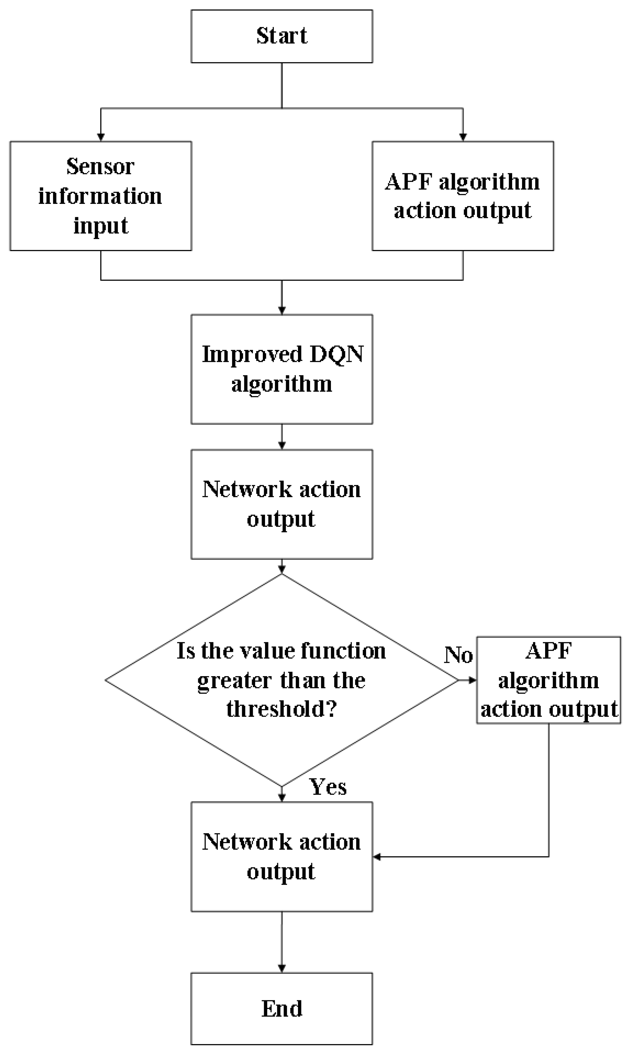
Set the $Q$ value threshold $Q_{limit}$, if the $Q$ function value that corresponds to the action $a_{max}$ selected for output by the algorithm in a state s is less than the threshold $Q_{limit}$, then the action $a_{real}$ is the information output by the APF; otherwise, $a_{real}$ is the action $a_{real}$ output by the neural network, as shown in Equation (14).

$$a_{real}=\left\{\begin{array}{cc}{a}_{max},\hfill & \hfill Q\left(\mathrm{s},a_{max};\theta \right)\ge Q_{limit}\\ \left[v_{apf},w_{apf}\right],\hfill & \hfill Q\left(\mathrm{s},a_{max};\theta \right)<Q_{limit}\end{array}\right..$$

(14)

The algorithm flow is shown in Figure 1.

2.5. Network Structure of Improved DQN Algorithm

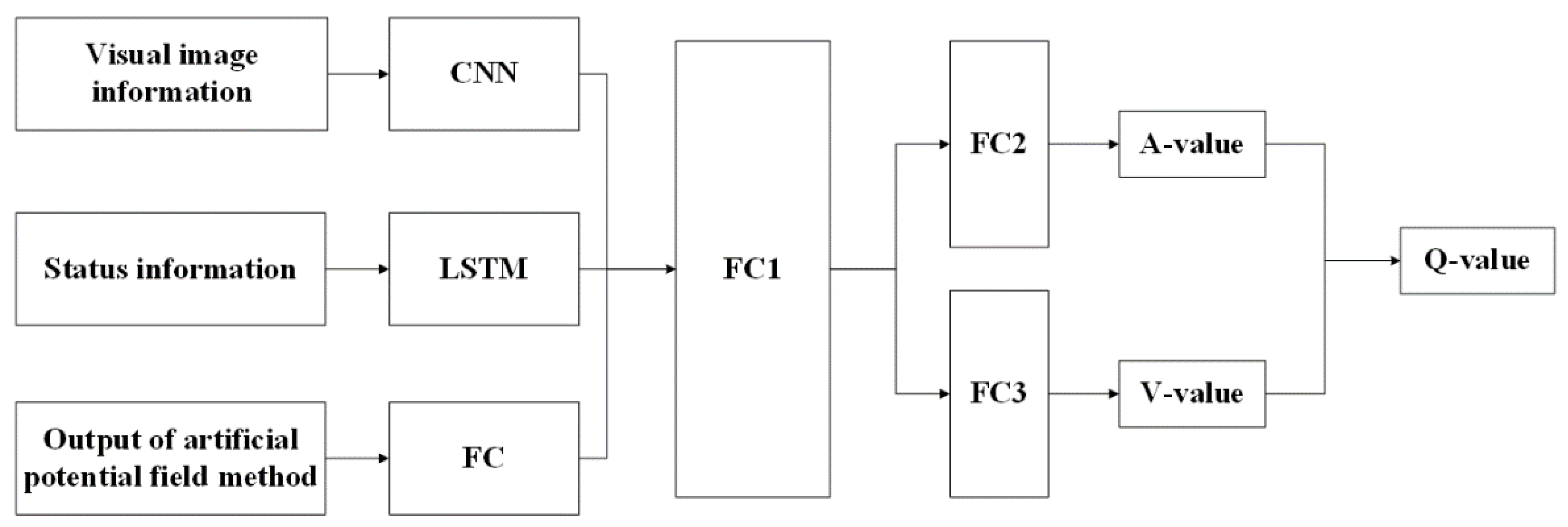
The network structure of the improved DQN algorithm is illustrated in Figure 2. The input to the network consists of three components: visual image information, state information, and APF action output. The state information incorporates lidar point cloud data and vehicle state information ${{\theta }_t,v}_t,w_t$. The visual image information is processed using a convolutional neural network to extract relevant feature information. The lidar point cloud information within the state information is passed through a LSTM network, which effectively captures dependencies across a long sequence of segments and strengthens the correlation between data. The action pairs output by the APF algorithm, serving as prior knowledge, undergo feature extraction through several fully connected layers. The network architecture incorporates the Dueling DQN algorithm, with fully connected layers producing the action dominance function and the value function. By combining these outputs, the algorithm generates the Q-value matrix for the action set A corresponding to the given state.

For visual image information, the improved DQN algorithm employs three convolutional layers for feature extraction. The dimensions of these layers are 8 × 8 × 4, 4 × 4 × 32, and 3 × 3 × 64, respectively. The number of output channels for the convolutional layers is 32, 64, and 64, respectively. The stride sizes for these layers are 4, 2, and 1, respectively. The convolutional layers utilize the “SAME” padding scheme to handle the image edges. Regarding the state information, the algorithm utilizes an LSTM network with a cell size of 256. The LSTM network is responsible for capturing the dependencies in the sequence of lidar point cloud data and reinforcing the correlation between the data segments. In an unknown environment, the LSTM can capture state information at different time steps to build a dynamic model of the environment. By passing current state, action, and reward information to the LSTM, it can learn the time-varying characteristics of the environment, enabling the intelligence to better understand the changes in the environment. The long-term memory properties of the LSTM allow it to remember previous states and action sequences so that long-term effects can be taken into account in path planning. This is useful for making decisions in complex environments where path planning often requires considering possible effects after multiple steps. LSTMs can consider both temporal and spatial information, thus improving the spatio-temporal sensitivity of the algorithm. In path planning, intelligence can predict possible future states and paths as well as select the best action based on the current state and historical trajectories. For the APF value information, two fully connected layers are employed for feature extraction. These layers consist of 200 and 100 neurons, respectively. The rectified linear unit (ReLU) function serves as the activation function for all layers. After processing the input data from the visual image, state information, and APF value, the Concat function is used to flatten the data into a one-dimensional vector. This vector is then split into two parts after passing through a fully connected layer. The output size for the action part is 1 × 9, and for the value part, it is 1 × 1. In visual image information processing, the relu activation function is mainly used; in LSTM networks, both activation functions sigmoid and tanh are used.

The ReLU activation function was born in 2011 and has been widely used in deep learning since its birth, as shown in Figure 3. The expression of the ReLU activation function is shown in Equation (15), which speeds up the training speed of the network, and the gradient is 1 when $x$ > 0, which can solve the problem of gradient vanishing. But, when $x$ ≤ 0, the function value is 0, and there is no activation effect; thus the function is not a function centered on 0.

$$f(x)=\{\begin{array}{cc}0\hfill & \hfill x\le 0\\ x\hfill & \hfill x>0\end{array}$$

(15)

The model thinned out by the RELU function can better mine the pixel features in the image that are beneficial for path planning, stabilize the convergence speed, and improve the convergence effect. The improved DQN algorithm is shown in

Table 1. Improved DQN algorithm flow.

Improved DQN Algorithm
Input: initialized empirical replay pool D, replay pool capacity N, є parameters, discount factor γ, learning rate α, number of training rounds epi, number of steps per round T, gradient descent minibatch as K, target network parameters update steps C
$\mathrm{Output}:\mathrm{Network}\mathrm{parameters}\theta$ $\mathrm{and}{\mathsf{\theta }}^{-}$
$\mathrm{Initialize}\mathrm{target}\mathrm{neural}\mathrm{network}\mathrm{and}\mathrm{estimated}\mathrm{neural}\mathrm{network}\mathrm{with}\mathrm{parameters}\theta$ $\mathrm{and}{\mathsf{\theta }}^{-}$ Initialize state s
for episode = 1:epi
for i = 1:T
$\mathrm{Use}\mathrm{the}\epsilon -$$\mathrm{greedy}\mathrm{strategy}\mathrm{to}\mathrm{select}\mathrm{action}{a}_t$ $\mathrm{with}\epsilon$ $\mathrm{probability};\mathrm{otherwise}\mathrm{select}{a_t=min}_{a}A(s_t,a;\theta )$             $\mathrm{Execute}\mathrm{action}{a}_t$ $\mathrm{in}\mathrm{state}{s}_t$$,\mathrm{the}\mathrm{next}\mathrm{state}\mathrm{is}{s}_{t+1}$ $\mathrm{and}\mathrm{the}\mathrm{reward}\mathrm{value}{r}_t$ is got
$\mathrm{Deposit}\mathrm{samples}(s_t,a_t,r_t,s_{t+1})$ $\mathrm{into}\mathrm{the}\mathrm{sample}\mathrm{pool}\mathrm{D}\mathrm{and}\mathrm{the}\mathrm{sampling}\mathrm{pool}$              $\mathrm{K}-1\mathrm{samples}(s_j,a_j,r_j,s_{j+1})$ $\mathrm{are}\mathrm{drawn}\mathrm{with}\mathrm{the}\mathrm{probability}\mathrm{of}\mathrm{random}\mathrm{sampling}\mathrm{in}\mathrm{sample}\mathrm{pool}\mathrm{D}$             $\mathrm{In}\mathrm{state}{s}_{t+1}$$,\mathrm{choose}\mathrm{the}\mathrm{action}{a}_{max}={min}_{a}A(s_{t+1},a;\theta )$
$\mathrm{Target}\mathrm{value}{y}_j=r_j+\mathsf{\gamma }(\mathrm{A}\left(s_{t+1},a_{max};{\beta ,\mathsf{\theta }}^{-}\right)+V\left(s_{t+1};{\mathsf{\theta }}^{-}\right)-\frac{1}{\left|A\right|}\sum _{a^{\mathrm{’}}}A(s,a^{\mathrm{’}};\beta ,\theta ))$
$\mathrm{Calculate}\mathrm{TD}-\mathrm{error}{\delta }_j$ $\mathrm{and}\mathrm{update}\mathrm{priority}{P\left(j\right)\leftarrow \phi }_j={\beta }_1{\delta }_i+{\beta }_2{r}_i+\epsilon$             The target network parameter θ$\mathrm{is}\mathrm{updated}\mathrm{by}\mathrm{gradient}\mathrm{descent}\mathrm{method}\mathrm{according}\mathrm{to}\mathrm{the}\mathrm{loss}\mathrm{function}\mathrm{using}\mathrm{MSE}\mathrm{error}$              $\mathrm{Update}\epsilon$ $\mathrm{based}\mathrm{on}\mathrm{cumulative}\mathrm{round}\mathrm{rewards}{R}_{sum}^L$
$\mathrm{if}\mathrm{T}\mathrm{\%}\mathrm{C}$$=0$              $\mathrm{Update}\mathrm{target}\mathrm{network}\mathrm{function}\theta \leftarrow {\mathsf{\theta }}^{-}$             end         end for         end for

.

3. Simulation

3.1. Simulation Environment

To evaluate the effectiveness of the improved algorithm, a simulation experiment was conducted using the Gazebo simulation environment. In this experiment, dynamic obstacles, representing personnel vehicles, were simplified, while static obstacles included goods and other items. Multiple path planning algorithms were tested to assess their efficiency and the quality of their path planning in various environments. The simulation experiment employed the following hardware configuration: CPU with a frequency of 2.9 GHz and a dynamic acceleration frequency of 4.2 GHz, 16 GB of memory, GPU with a default frequency of 1365 MHz, and a maximum Boost frequency of 1680 MHz. The software platform consisted of the Ubuntu 18.04 operating system, Visual Studio Code development environment, Python and C++ programming languages, Robot Operating System (ROS) Melodic, Gazebo simulation platform, TensorFlow 1.12.0 deep learning framework, CUDA 9.0, cuDNN, and the OpenCV 3.1.0.0 computer vision library, among others.

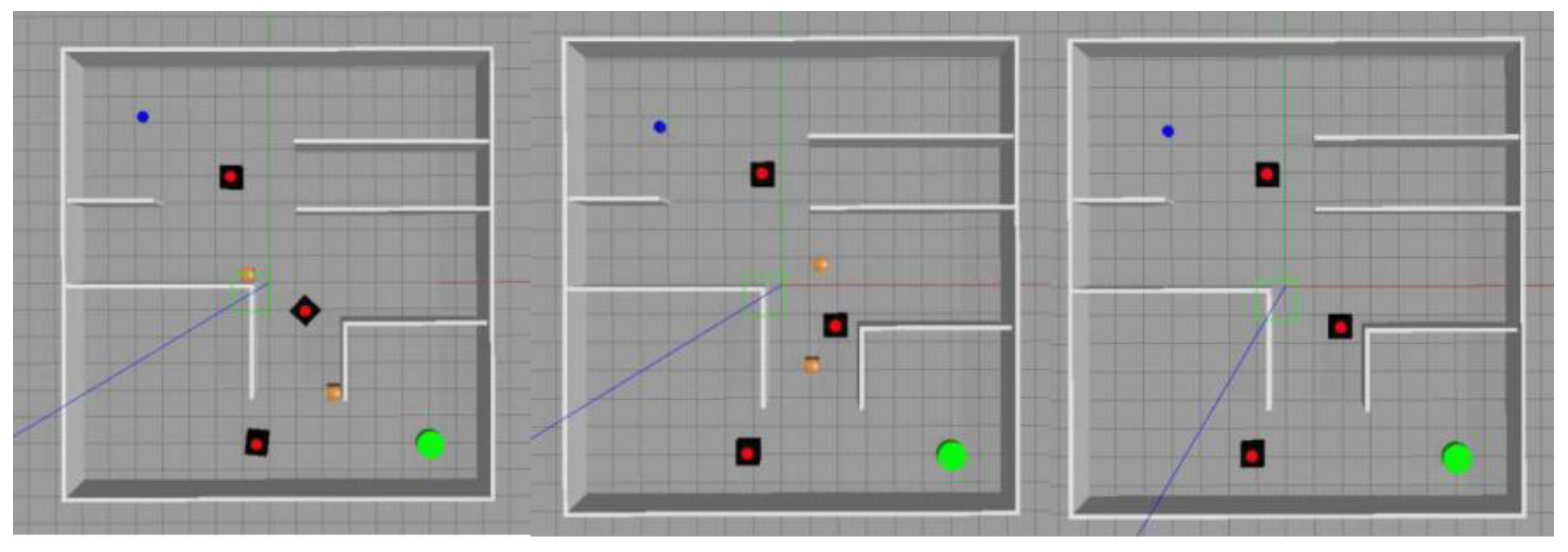
To fully verify the algorithm, obstacle-free environments, wide obstacle environments, and complex dynamic environments were built separately, as shown in Figure 4a–c.

In all environments, the dimensions of the vehicle are 0.42 m in length, 0.31 m in width, and 0.184 m in height. Specifically, the obstacle-free environment has a size of 20 m × 20 m, and, at the beginning of each round, the starting position of the autonomous vehicle is randomly determined, as is the target position. The obstacle environment consists of an infinitely large map with a 20 m × 20 m obstacle area. It includes five static squares with dimensions of 1 m × 1 m × 1 m as obstacles, along with ten dynamic squares representing people, vehicles, and other moving obstacles in an open environment. The size of static squares is 1 m × 1 m × 1 m. The complex dynamic environment is 15 m × 15 m in size, with three square cubes with wheels of 1 m × 1 m × 1 m as dynamic obstacles, and two static obstacles with a length of 0.54 m, a width of 0.31 m, and a height of 0.019 m. Black and wooden squares are simulation models of dynamic obstacles and static obstacles, respectively. The simulation also includes blue dots representing the autonomous vehicle, green dots representing the target points (transparent non-obstacles), red paths representing the driving paths of the autonomous vehicle, and blue, green, and yellow paths representing the driving paths of dynamic obstacles. At the start of each round, the starting position of the static obstacle is randomly determined, whereas the dynamic obstacle has a fixed starting point but follows a random walking path. The maximum linear speed of the dynamic obstacles is 0.5 m/s. In traditional algorithms, the maximum linear speed of the autonomous vehicle is set to 1 m/s, and the angular speed is 0.5 rad/s. The experiment utilizes Jackal autonomous vehicles for path planning, which are equipped with a single-line lidar, a binocular camera, an odometer, and two drive wheels. The point cloud information dimension of the single-line lidar is 360°, and its detection distance is between 0.1 m and 3.5 m. The binocular camera captures RGB image information with a resolution of 768 × 1024 × 3.

3.1.1. State and Action Space Definition

Define a quadruple [${{\theta }_t,v}_t,w_t,d_t$], where $v_t,w_t$ represent the linear and angular velocity information of the autonomous vehicle at time t, respectively; ${\theta }_t$ represents the angle information of the autonomous vehicle relative to the target point; and $d_t$ represents the distance information of the autonomous vehicle relative to the target point. The main actions of the autonomous vehicle can be divided into combinations of discrete values of linear velocity V and angular velocity W. The action space is defined to ensure that the actions of the autonomous vehicle are coherent and comply with kinematic constraints, see

Table 2. State and action space definition.

Action	Linear Velocity V	Angular Velocity W
0	1 m/s	−1 rad/s
1	1 m/s	−0.5 rad/s
2	1 m/s	0 rad/s
3	1 m/s	0.5 rad/s
4	1 m/s	1 rad/s
5	0 m/s	0 rad/s
6	−0.5 m/s	−0.5 rad/s
7	−0.5 m/s	0 rad/s
8	−0.5 m/s	0.5 rad/s

.

For the state space, we choose the visual image state information, its own position and velocity state information, and APF algorithm action output state information. The visual image state information can provide the unmanned vehicle with the situation of the surrounding obstacles and provide some action basis for its path planning; the self-position and velocity state information can provide the unmanned vehicle with its accurate state and provide the initial conditions for the action output at the current moment. The action space includes 9 discrete values, respectively, for the unmanned vehicle’s forward, stop, and steering to provide a more comprehensive action to drive more smoothly.

3.1.2. Reward Function Definition

This article aims at the characteristics of reinforcement learning, combined with heuristic methods to define a distance-based reward function, as shown in Equations (16) and (17).

The reward function mainly consists of two major modules; the first one is based on the distance of the end point of the reward mechanism, and the second one is based on the distance of the reward mechanism with the target obstacle. The reward mechanism based on the distance can make the unmanned vehicle have better rewards when it is closer to the target point, and negative rewards when it is far away from the target point or when it is loitering; the reward mechanism based on the distance to the target obstacle can make the unmanned vehicle have higher negative rewards when it is closer to the obstacle. The reward function that combines the two enables the unmanned vehicle to reach the target point quickly while staying away from the obstacle.

$$r_t=\left\{\begin{array}{cc}\frac{\left(r+r_{ob}\right)\ast (d_g-d_t)}{d_g}\hfill & \hfill d_g\ge d_t\\ -1\hfill & \hfill d_g<d_t\end{array}\right.,$$

(16)

where $d_t=\sqrt{{(x_t-x_e)}^2+{(y_t-y_e)}^2}$ and $d_g=\sqrt{{(x_0-x_e)}^2+{(y_0-y_e)}^2}$ represent the distance between the autonomous vehicle and the end point at time t and the distance between the starting point and the end point, respectively. $x_t$ and $y_t$ represent the coordinate points of the autonomous vehicle in the global coordinate system. ${(x}_0,y_0)$ represents the starting point coordinates, and ${(x}_e,y_e)$ represents the end-point coordinates.

$$r=\left\{\begin{array}{cc}20\hfill & \mathrm{R}\mathrm{e}\mathrm{a}\mathrm{c}\mathrm{h}\mathrm{i}\mathrm{n}\mathrm{g}\mathrm{t}\mathrm{h}\mathrm{e}\mathrm{t}\mathrm{a}\mathrm{r}\mathrm{g}\mathrm{e}\mathrm{t}\mathrm{p}\mathrm{o}\mathrm{i}\mathrm{n}\mathrm{t}\hfill \\ -0.015\hfill & \mathrm{R}\mathrm{o}\mathrm{t}\mathrm{a}\mathrm{t}\mathrm{e}\mathrm{o}\mathrm{r}\mathrm{r}\mathrm{e}\mathrm{m}\mathrm{a}\mathrm{i}\mathrm{n}\mathrm{s}\mathrm{t}\mathrm{a}\mathrm{t}\mathrm{i}\mathrm{o}\mathrm{n}\mathrm{a}\mathrm{r}\mathrm{y}\mathrm{i}\mathrm{n}\mathrm{p}\mathrm{l}\mathrm{a}\mathrm{c}\mathrm{e}\hfill \\ 0.01\hfill & \mathrm{O}\mathrm{t}\mathrm{h}\mathrm{e}\mathrm{r}\mathrm{s}\hfill \end{array}\right.,$$

(17)

where $r_t$ represents the immediate reward at time $t$, which is a function with the distance function as the denominator and the reward function $r+r_{ob}$ as the numerator. For situations where the autonomous vehicle encounters obstacles, does not move or spins out of the map, or does not meet expectations, a negative reward is given as punishment. The autonomous vehicle is rewarded when it reaches the target point. The farther the distance, the larger the $\left|r_t\right|$, the closer the distance, the smaller the $\left|r_t\right|$. In other cases, a small negative value is given to allow the autonomous vehicle to complete the target task in as few steps as possible. To keep the autonomous vehicle as far away from obstacles as possible, the dilation radii $d_{min1}$, $d_{min2}$, and $d_{min3}$ are set around the obstacles. This article sets their parameter values to −0.3, −0.5, and −1, respectively. As the distance $d_{ob}$ between the autonomous vehicle and the obstacle decreases, the penalty value gradually increases to −1, as shown in Equation (18).

$$r_{ob}=\left\{\begin{array}{cc}\frac{-d_{min3}}{4d_{ob}}\hfill & \hfill d_{min2}\le d_{ob}<d_{min1}\\ \frac{-d_{min3}}{2d_{ob}}\hfill & \hfill d_{min3}\le d_{ob}<d_{min2}\\ -1\hfill & \hfill d_{ob}<d_{min3}\\ 0\hfill & \hfill d_{ob}>d_{min1}\end{array}\right.$$

(18)

3.1.3. Algorithm Parameter Settings

The algorithm parameter settings and the sequence numbers of each algorithm are shown in

Table 3. Parameter settings for path planning algorithm.

Parameter	Meaning	Value
${\mathit{\epsilon }}_{\mathit{m}\mathit{a}\mathit{x}}$	maximum greed factor	0.2
$\mathit{\mu }$	exploring factors	0.01
α	learning rate	0.0001
${\mathit{a}}_{\mathit{s}}$	importance adopts priority parameters	0.4
${\mathit{\beta }}_{\mathit{s}}$	importance sampling scale factor parameter	0.6
γ	reward discount coefficient	0.98
$\mathit{\sigma }$	experience playback reward weight	0.1
$\mathrm{epi}$	maximum number of training rounds	300
$\mathrm{Max}\text{\_}\mathrm{step}$	maximum training steps	50,000
$\mathrm{K}$	gradient descent parameter	32
$\mathrm{C}$	target network update steps	5
${\mathit{Q}}_{\mathit{l}\mathit{i}\mathit{m}\mathit{i}\mathit{t}}$	lower limit of action output Q value	−0.1
${\mathit{v}}_{\mathit{l}\mathit{i}\mathit{m}}$	upper limit of potential field function velocity	1.0
${\mathit{w}}_{\mathit{l}\mathit{i}\mathit{m}}$	upper limit of the angular velocity of the potential field function	0.5
${\mathit{k}}_{\mathit{x}},{\mathit{k}}_{\mathit{y}}$	force field weight parameters	0.7

and

Table 4. Algorithm number.

Algorithm Number	Algorithm Name
Algorithm 1	Dueling DQN Algorithm
Algorithm 2	DQN Algorithm
Algorithm 3	Double DQN Algorithm
Algorithm 4	D3QNPER Algorithm
Algorithm 5	APF-D3QNPER Algorithm
Algorithm 6	A*+DWA Algorithm
Algorithm 7	A*+TEB Algorithm

, respectively.

We defined Dueling DQN Algorithm as Algorithm 1, DQN Algorithm as Algorithm 2, Double DQN Algorithm as Algorithm 3, D3QNPER Algorithm as Algorithm 4, APF-D3QNPER Algorithm as Algorithm 5, A*+DWA Algorithm as Algorithm 6 and A*+TEB Algorithm as Algorithm 7, as shown in Table 4.

3.2. Simulation

3.2.1. Non-Obstruction Scenarios

The starting point and end point of the autonomous vehicle are randomly selected in an infinite map range. Since Algorithms 1–4 are all variants of DQN, and their performance differences after training to convergence are not significant, we focus on comparing the planning time and planning path length between Algorithms 4 and 5 in the obstacle-free scenario. To conduct this comparison, we utilize five sets of starting and ending points as test environments. For detailed results, please refer to

Table 5. Environmental points.

Environment Number	Starting Point Coordinates (m)	End Point Coordinates (m)	$\mathbf{Initial}\mathbf{Angle}(°$)
1	(1.12, −8.63)	(−13.78, −3.08)	3.11
2	(1.44, 9.52)	(−11.27, −7.50)	−0.06
3	(−8.23, 9.23)	(−4.69, −1.47)	−2.50
4	(−12.36, 1.34)	(12.70, −1.06)	2.64
5	(6.73, −1.30)	(−7.72, 8.49)	0.56

.

The test was conducted using five sets of test environments, and each environment was tested for 20 rounds. The results were averaged to obtain the performance metrics. Specifically, we compared the planning time and planning path length between Algorithms 4 and 5 in these five test environments. The detailed comparison results can be found in

Table 6. Planning time.

	Env 1 (s)	Env 2 (s)	Env 3 (s)	Env 4 (s)	Env 5 (s)
Algorithm 4	13.420	13.566	4.828	6.713	6.870
Algorithm 5	7.743	5.527	3.876	5.668	3.897

and

Table 7. Planning path length.

	Env 1 (m)	Env 2 (m)	Env 3 (m)	Env 4 (m)	Env 5 (m)
Algorithm 4	66.44	61.19	31.83	48.44	37.69
Algorithm 5	29.72	42.18	31.45	46.86	33.32

.

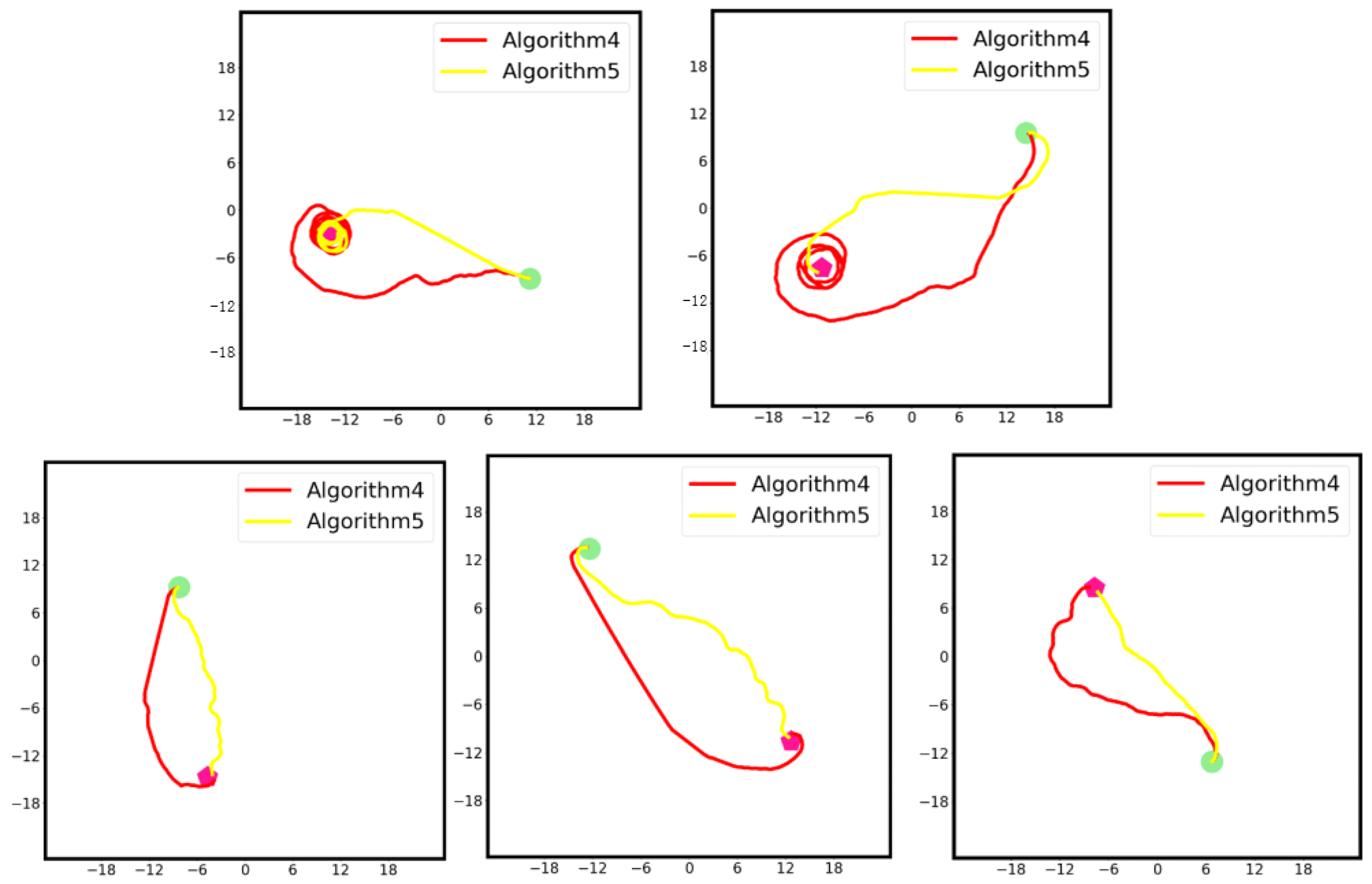
The walking paths of Algorithms 4 and 5 in the five rounds of random environment tests are shown in Figure 5.

As can be seen from Table 7 and

Table 8. Static obstacle points information.

	Static Obstacle Number
	1	2	3	4	5
Coordinate (m)	(4.0, 1.0)	(3.8, 1.0)	(−10.0, −8.0)	(−10.0, 4.0)	(7.0, 2.0)

, as well as Figure 5, in the five rounds of random environments, the APF-D3QNPER algorithm (Algorithm 5) achieved an average driving time of 5.342 s and an average planning path length of 31.978 m. When compared with Algorithm 4, the APF-D3QNPER algorithm demonstrated a 41.16% reduction in driving time and a 34.85% reduction in planning path length. In an obstacle-free environment, where the optimal solution is a straight-line distance from the starting point to the end point, the planning route generated by the APF-D3QNPER algorithm exhibits closer alignment with a straight line, resulting in improved performance.

3.2.2. Obstacle Environment Scenarios

In an obstacle-free environment, the APF-D3QNPER algorithm demonstrates a superior performance compared to other DQN and its derived algorithms. It achieves higher reward values in shorter training times and exhibits relatively low total loss during the training process. To further evaluate the obstacle avoidance ability of the APF-D3QNPER algorithm, a comparison is made with Algorithm 4. By comparing the performance of the APF-D3QNPER algorithm with Algorithm 4, we can verify the effectiveness of the APF-D3QNPER algorithm in terms of obstacle avoidance.

In this simulation, the static obstacle is placed at a fixed position, as indicated in Table 8. The dynamic obstacle also has a fixed starting position but follows a random driving path. The minimum distance between obstacles is maintained at 5 m apart. To assess the obstacle avoidance ability of the algorithm, five rounds of tests are conducted.

Table 9. Dynamic obstacle points information.

Environment	Coordinate (m)	Dynamic Obstacle Number
		1	2	3	4	5
Env 1	$cc$	−9.099	2.012	−13.483	0.199	−10.104
	$y$	−11.562	10.575	−11.825	−5.842	−0.648
Env 2	$x$	−4.105	−5.356	1.036	−11.294	2.471
	$y$	−1.913	5.383	5.106	−3.613	−7.456
Env 3	$x$	9.870	1.162	5.208	−4.766	1.636
	$y$	10.960	6.508	−10.065	−6.276	11.270
Env 4	$x$	−10.723	13.674	14.438	11.899	2.262
	$y$	−8.629	−2.413	1.724	−11.664	−12.032
Env 5	$x$	6.089	−5.218	−13.275	9.756	1.148
	$y$	−6.932	3.602	−8.044	5.578	14.735

shows dynamic obstacle points information.

Table 10. Dynamic obstacle points information.

Environment	Coordinate (m)	Dynamic Obstacle Number
		6	7	8	9	10
Env 1	$x$	−7.417	−11.573	−14.959	−5.253	14.099
	$y$	−3.343	6.833	7.881	−11.140	−3.405
Env 2	$x$	2.551	8.424	9.998	−9.033	9.428
	$y$	10.639	8.505	−7.697	8.490	−12.164
Env 3	$x$	0.562	6.270	6.427	−13.812	12.791
	$y$	−10.467	11.200	7.159	2.218	2.460
Env 4	$x$	5.577	8.347	−14.126	10.805	14.843
	$y$	2.145	5.429	5.661	−8.730	5.579
Env 5	$x$	−11.071	8.007	11.488	−14.740	−12.999
	$y$	11.938	1.794	−7.051	11.176	−1.302

shows dynamic obstacle points information.

The tests include five sets of test environments. We tested each environment for 20 rounds, took the average of the test results, and compared the planning time and planning path length of Algorithms 4 and 5 in the five test environments, as shown in

Table 11. Average planning time.

	Env 1 (s)	Env 2 (s)	Env 3 (s)	Env 4 (s)	Env 5 (s)
Algorithm 4	16.753	13.705	9.011	10.362	12.854
Algorithm 5	6.161	9.355	10.476	9.194	11.643

and

Table 12. The average length of the planned path.

	Env 1 (m)	Env 2 (m)	Env 3 (m)	Env 4 (m)	Env 5 (m)
Algorithm 4	39.753	52.673	40.101	54.611	43.505
Algorithm 5	29.344	48.182	31.453	48.134	33.324

.

In the conducted test, the APF-D3QNPER algorithm achieved an average driving time of 9.365 s and an average driving path length of 38.082 m. When compared to Algorithm 4, the APF-D3QNPER algorithm exhibited a 25.23% reduction in driving time and a 17.44% reduction in planning path length. During the experiment, collisions between autonomous vehicles occurred due to the presence of a large number of obstacles and their random movements, resulting in planning failures. The failure rate of obstacle avoidance serves as a crucial indicator to evaluate the obstacle avoidance ability of autonomous vehicles. Table 12 provides the number of failures for Algorithms 4 and 5 across five different environments.

As shown in

Table 13. Failure times of path planning.

	Env 1 (Times)	Env 2 (Times)	Env 3 (Times)	Env 4 (Times)	Env 5 (Times)
Algorithm 4	3	3	5	1	2
Algorithm 5	1	0	0	0	1

, in the obstacle environment, the overall average failure rate of algorithm 4 is 13%, and the overall average failure rate of Algorithm 5 is 2%, which has a relatively obvious improvement in obstacle avoidance ability.

3.2.3. Dynamic and Complex Environmental Planning Scenarios

To further validate the generalization ability of the APF-D3QNPER algorithm and ensure its effectiveness in avoiding diverse obstacles within unknown complex environments, this study will conduct simulations in a complex dynamic environment. This environment will include three dynamic obstacles representing people walking and two static obstacles representing fixed objects. Additionally, the number of walls will be increased to simulate a wall-filled environment. The performance of the APF-D3QNPER algorithm will be compared with traditional map-based path planning algorithms to evaluate its planning effectiveness and efficacy in such scenarios.

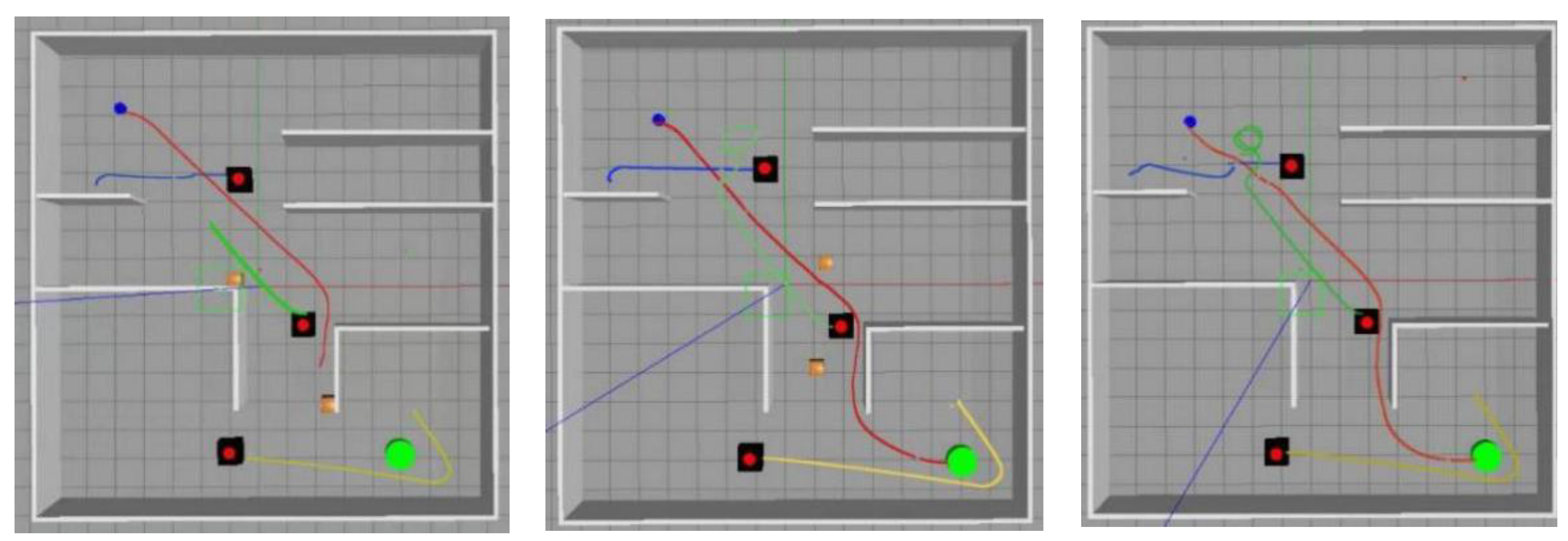
This article employs a fixed environment map with dimensions of 15 m × 15 m. The starting positions of the dynamic obstacles are consistent across the environments, while their driving paths are randomized. The positions of the static obstacles vary in the three different environments. The dynamic obstacles maintain a fixed speed of 0.5 m/s, while the maximum driving speed of the autonomous vehicle is set at 1 m/s, with an angular speed of 0.5 rad/s. To ensure statistical robustness, each group of three environments is tested twenty times, and the average results are taken as a reference. The complex dynamic simulation environment is illustrated in Figure 6, and the positions of the three environment groups can be found in

Table 14. Static obstacle points information.

Environment Number	Obstacle 1 Coordinates (m)	Obstacle 2 Coordinates (m)
1	None	None
2	(1.378, 0.743)	(1.221, −2.801)
3	(2.462, −3.803)	(−0.749, 0.336)

and

Table 15. List of dynamic obstacle points.

Dynamic Obstacle Number	Coordinate (m)
1	(−0.482, 3.881)
2	(2.028, −1.370)
3	(−1.258, −5.761)

.

The path planning results are shown in

Table 16. The average length of planned paths between this algorithm and traditional algorithms.

	Env 1 (m)	Env 2 (m)	Env 3 (m)
Algorithm 4	26.433	26.543	24.278
Algorithm 5	25.233	25.512	24.459
Algorithm 6	26.122	25.389	24.513
Algorithm 7	24.183	25.329	22.627

,

Table 17. Planning time between this algorithm and traditional algorithms.

	Env 1 (s)	Env 2 (s)	Env 3 (s)
Algorithm 4	10.542	13.564	7.732
Algorithm 5	9.481	12.571	7.198
Algorithm 6	43.418	44.257	40.079
Algorithm 7	33.142	32.241	38.513

and

Table 18. Failure times of algorithm path planning.

	Env 1 (Times)	Env 2 (Times)	Env 3 (Times)
Algorithm 4	3	4	3
Algorithm 5	1	1	0
Algorithm 6	6	5	7
Algorithm 7	5	5	6

.

The algorithm proposed in this article builds upon the foundation of Algorithm 4 and further enhances the planning effectiveness. In each environment, the average planning length is approximately 25.07 m, and the average path planning time is 9.75 s. These results demonstrate that the algorithm achieves shorter planning lengths and faster planning times compared to other algorithms. Additionally, the algorithm exhibits fewer errors in terms of planning failures. Specifically, when compared to Algorithm 4, algorithm 5 showcases a 75.19% reduction in the failure rate, indicating a significant performance improvement. As a result, the overall planning effect of the algorithm presented in this article demonstrates clear advantages over alternative approaches.

The planning results of Algorithms 4–7 in the three environments are shown in Figure 7, Figure 8, Figure 9 and Figure 10.

In Figure 7, Figure 8, Figure 9 and Figure 10, the visualization of the complex dynamic environment is depicted. The black squares represent dynamic obstacles, while the wooden squares represent static obstacles. The blue dots represent the simulation model of the autonomous vehicle, and the green dots indicate the position of the end point. The red paths represent the driving path of the autonomous vehicle, while the blue, green, and yellow paths represent the driving paths of dynamic obstacles. In summary, when considering a complex dynamic environment, map-based path planning algorithms demonstrate satisfactory obstacle avoidance capabilities for static obstacles within the map. However, they often struggle with avoiding dynamic obstacles, resulting in longer planning times and a higher likelihood of planning failures. On the other hand, the algorithm proposed in this article exhibits significant advantages in avoiding both static and dynamic obstacles. It also achieves shorter planning times, making it better suited for real-world planning scenarios.

In these obstacle scenarios, the start point and the end point used in this paper are all randomly generated coordinate values, and the walking paths of the dynamic obstacles are randomized. During the testing process, the unmanned vehicles using the APF-D3QNPRE algorithm can avoid all the obstacles and arrive at the end point smoothly, which fully demonstrates the generalization ability of the APF-D3QNPRE algorithm.

4. Conclusions

At present, traditional path planning algorithms for autonomous vehicles heavily rely on high-precision maps to generate routes. However, in obstacle-free and expansive environments, the mapping results may be inadequate, leading to suboptimal or even non-feasible driving paths. Additionally, conventional DQN DRL algorithms tend to converge slowly or fail to converge during training. To address these challenges, this article presents the APF-D3QNPER algorithm along with an improved network structure and an appropriate reward function. The algorithm is evaluated through simulation experiments and further validated by implementing it in a real autonomous vehicle system to assess its performance in unknown environments. The results demonstrate the algorithm’s superiority and its potential for practical applications.

The contributions and innovations of this paper include the following:

(1)

To enhance the convergence ability of the traditional DRL algorithm, this study introduces a modified approach for assigning rewards to experience samples during the experience replay phase. Specifically, the TD error and a weighted sum are employed as sampling probabilities for prioritized experience sampling. This prioritization method improves the overall convergence performance of the algorithm.

(2)

By integrating an action output method based on the APF algorithm with the D3QNPER algorithm, this study achieves improved convergence speed, as well as enhanced obstacle avoidance and generalization capabilities for autonomous vehicles operating in complex dynamic environments.

(3)

Adding an LSTM network to the state feature extraction network and inputting state data between several frames before and after into the LSTM network simultaneously further improves its adaptability in unknown environments and enhances its spatiotemporal sensitivity to the environment.

This paper validates the effectiveness of the APF-D3QNPER algorithm through simulation experiments. Currently, the action output of the algorithm is discrete with multiple values. In future research, the consideration of continuous actions can be explored to achieve smoother driving paths. For unmanned vehicles or small unmanned mobile robots, the limited movement output will affect their maneuvering performance seriously. Continuous action can make the path smoother, reduce the jitter generated by the movement and improve the comfort level, further improve the obstacle avoidance ability, and passing performance, and protect the safety of the vehicle carrying people or objects. The D3QNPRE algorithm is an improved algorithm based on the DQN, which outputs a limited Q-value, and therefore cannot output continuous action; so, in the subsequent improvement process, the combination of the policy function and the value function should be considered for the deep reinforcement learning algorithm to solve it. Additionally, conducting experiments in real-world environments can provide further insights and validation. In the future, the APF-D3QNPRE algorithm can be applied to multiple domains in real-world scenarios. In the field of autonomous vehicles, it can help autonomous vehicles with more accurate path planning and decisions, enabling them to drive safely in different traffic situations, avoid accidents, and choose the best route more efficiently. In the field of drones, they can be used to plan the flight paths of drones so that they can accomplish tasks in complex environments, such as search and rescue, agricultural inspections, and cargo transportation. In the fields of logistics and warehousing, it can be used to optimize the transportation path of goods and the operation process inside the warehouse to improve efficiency and reduce costs. In the field of intelligent robots, it helps robots to perform tasks in various environments, such as cleaning, food delivery, medical assistance, etc., while avoiding obstacles and interacting with human users. Moreover, while the DRL algorithm introduced in this paper primarily utilizes value functions for training, future research can explore incorporating methods based on policy functions or a combination of policy functions and value functions. These approaches have the potential to enhance the algorithm’s adaptability to different environmental conditions.

References

- Ma, X.; Gao, M.; Wang, X. A Summary of the current situation of driverless vehicles in the world. Comput. Knowl. Technol. 2019, 15, 189–190. [Google Scholar]
- Wang, J.; Gao, J.; Zhong, X. Analysis of the development and problems of driverless vehicles. Automob. Parts 2020, 1, 89–91. [Google Scholar]
- Jin, Y. Minimum time planning model of robot path for avoiding obstacles in the static field. Mach. Tool Hydraul. 2018, 4, 88–93. [Google Scholar]
- Qi, Z. Study on Lane-Changing and Overtaking Control Method of Autonomous Vehicle; D. Yanshan University: Qinhuangdao, China, 2017. [Google Scholar]
- Yu, Z.; Li, Y.; Xiong, L. A review of the motion planning problem of autonomous vehicle. J. Tongji Univ. (Nat. Sci.) 2017, 45, 1150–1159. [Google Scholar]
- Abdallaoui, S.; Aglzim, E.; Chaibet, A.; Kribèche, A. Thorough review analysis of safe control of autonomous vehicles: Path planning and navigation techniques. Energies 2022, 15, 1358. [Google Scholar] [CrossRef]
- Cao, H.; Song, X.; Huang, Z.; Pan, L. Simulation research on emergency path planning of an active collision avoidance system combined with longitudinal control for an autonomous vehicle. Proc. Inst. Mech. Eng. Part D J. Automob. Eng. 2016, 230, 1624–1653. [Google Scholar] [CrossRef]
- Ji, J.; Khajepour, A.; Melek, W.W.; Huang, Y. Path planning and tracking for vehicle collision avoidance based on model predictive control with multiconstraints. IEEE Trans. Veh. Technol. 2016, 66, 952–964. [Google Scholar] [CrossRef]
- Grandia, R.; Jenelten, F.; Yang, S.; Farshidian, F.; Hutter, M. Perceptive Locomotion through Nonlinear Model-Predictive Control. arXiv 2022, arXiv:2208.08373. [Google Scholar] [CrossRef]
- Domina, Á.; Tihanyi, V. LTV-MPC approach for automated vehicle path following at the limit of handling. Sensors 2022, 22, 5807. [Google Scholar] [CrossRef]
- Wang, X.; Liu, J.; Peng, H.; Qie, X.; Zhao, X.; Lu, C. A simultaneous planning and control method integrating APF and MPC to solve autonomous navigation for USVs in unknown environments. J. Intell. Robot. Syst. 2022, 105, 36. [Google Scholar] [CrossRef]
- Mahesh, B. Machine learning algorithms—A review. Int. J. Sci. Res. 2020, 9, 381–386. [Google Scholar]
- Smart, W.D.; Kaelbling, L.P. Practical reinforcement learning in continuous spaces. In Proceedings of the Seventeenth International Conference on Machine Learning, ICML, San Francisco, CA, USA, 29 June–2 July 2000; pp. 903–910. [Google Scholar]
- Recht, B. A tour of reinforcement learning: The view from continuous control. Annu. Rev. Control Robot. Auton. Syst. 2019, 2, 253–279. [Google Scholar] [CrossRef]
- Dcrhami, V.; Majd, V.J.; Ahmadabadi, M.N. Fuzzy Sarsa Learning and the proof of the existence of its stationary points. Asian J. Control 2008, 10, 535–549. [Google Scholar] [CrossRef]
- Mnih, V.; Kavukcuoglu, K.; Silver, D.; Graves, A.; Antonoglou, I.; Wierstra, D.; Riedmiller, M. Playing atari with deep reinforcement learning. arXiv 2013, arXiv:1312.5602. [Google Scholar]
- Nair, A.; Srinivasan, P.; Blackwell, S.; Alcicek, C.; Fearon, R.; De Maria, A.; Panneershelvam, V.; Suleyman, M.; Beattie, C.; Petersen, S.; et al. Massively parallel methods for deep reinforcement learning. arXiv 2015, arXiv:1507.04296. [Google Scholar]
- Van Hasselt, H.; Guez, A.; Silver, D. Deep reinforcement learning with double q-learning. In Proceedings of the AAAI Conference on Artificial Intelligence, Phoenix, Arizona, 12–17 February 2016. [Google Scholar] [CrossRef]
- Wang, Z.; Schaul, T.; Hessel, M.; Hasselt, H.; Lanctot, M.; Freitas, N. Dueling network architectures for deep reinforcement learning. In Proceedings of the International Conference on Machine Learning. PMLR, New York, NY, USA, 19–24 June 2016; pp. 1995–2003. [Google Scholar]
- Anschel, O.; Baram, N.; Shimkin, N. Averaged-DQN: Variance reduction and stabilization for deep reinforcement learning. In Proceedings of the International Conference on Machine Learning, PMLR, Sydney, Australia, 6–11 August 2017; pp. 176–185. [Google Scholar]
- Dong, Y.; Yang, C.; Dong, Y.; Qu, X.; Xiao, H.; Wang, Z. Robot Path Planning based on improved DQN. Comput. Eng. Des. 2021, 42, 552–558. [Google Scholar]
- Hausknecht, M.; Stone, P. Deep recurrent Q-learning for partially observable MDPs. In Proceedings of the Association for the Advance of Artificial Intelligence Fall Symposium, Palo Alto, CA, USA, 23 July 2015; pp. 29–37. [Google Scholar]
- Schaul, T.; Quan, J.; Antonoglou, I.; Silver, D. Prioritized experience replay. arXiv 2015, arXiv:1511.05952. [Google Scholar]
- Liu, P. Research on Optimization Method of Deep Reinforcement Learning Experience Replay; D. China University of Mining and Technology: Jiangsu, China, 2021. [Google Scholar]
- Bae, H.; Kim, G.; Kim, J.; Qian, D.; Lee, S. Multi-robot path planning method using reinforcement learning. Appl. Sci. 2019, 9, 3057. [Google Scholar] [CrossRef]
- Tai, L.; Liu, M. Towards cognitive exploration through deep reinforcement learning for mobile robots. arXiv 2016, arXiv:1610.01733. [Google Scholar]
- Lei, X.; Zhang, Z.; Dong, P. Dynamic path planning of unknown environment based on deep reinforcement learning. J. Robot. 2018, 2018, 5781591. [Google Scholar] [CrossRef]
- Tiong, T.; Saad, I.; Teo, K.T.K.; bin Lago, H. Autonomous vehicle driving path control with deep reinforcement learning. In Proceedings of the IEEE 13th Annual Computing and Communication Workshop and Conference (CCWC), Las Vegas, NV, USA, 8–11 March 2023. [Google Scholar] [CrossRef]
- Du, Y.; Chen, J.; Zhao, C.; Liu, C.; Liao, F.; Chan, C.Y. Comfortable and energy-efficient speed control of autonomous vehicles on rough pavements using deep reinforcement learning. Transp. Res. Part C Emerg. Technol. 2022, 134, 103489. [Google Scholar] [CrossRef]
- Li, G.; Yang, Y.; Li, S.; Qu, X.; Lyu, N.; Li, S.E. Decision making of autonomous vehicles in lane change scenarios: Deep reinforcement learning approaches with risk awareness. Transp. Res. Part C Emerg. Technol. 2022, 134, 103452. [Google Scholar] [CrossRef]
- Pop, A.; Pop, N.; Tarca, R.; Lung, C.; Sabou, S. Wheeled mobile robot H.I.L. interface: Quadrature encoders emulation with a low cost dual-core microcontroller. In Proceedings of the 2023 17th International Conference on Engineering of Modern Electric Systems (EMES), Oradea, Romania, 9–10 June 2023; pp. 1–4. [Google Scholar] [CrossRef]
- Song, B.; Wang, Z.; Zou, L. An improved PSO algorithm for smooth path planning of mobile robots using continuous high-degree Bezier curve. Appl. Soft Comput. 2021, 100, 106960. [Google Scholar] [CrossRef]
- Zhang, H.; Lin, W.; Chen, A. Path Planning for the Mobile Robot: A Review. Symmetry 2018, 10, 450. [Google Scholar] [CrossRef]
- Hart, P.; Nilsson, N.; Raphael, B. A Formal Basis for the Heuristic Determination of Minimum Cost Paths. IEEE Trans. Syst. Sci. Cybern. 1968, 4, 100–107. [Google Scholar] [CrossRef]
Figure 1.
Algorithm flow.