An Evolutionary Neural Network Approach for Slopes Stability Assessment

Abstract

A current big challenge for developed or developing countries is how to keep large-scale transportation infrastructure networks operational under all conditions. Network extensions and budgetary constraints for maintenance purposes are among the main factors that make transportation network management a non-trivial task. On the other hand, the high number of parameters affecting the stability condition of engineered slopes makes their assessment even more complex and difficult to accomplish. Aiming to help achieve the more efficient management of such an important element of modern society, a first attempt at the development of a classification system for rock and soil cuttings, as well as embankments based on visual features, was made in this paper using soft computing algorithms. The achieved results, although interesting, nevertheless have some important limitations to their successful use as auxiliary tools for transportation network management tasks. Accordingly, we carried out new experiments through the combination of modern optimization and soft computing algorithms. Thus, one of the main challenges to overcome is related to the selection of the best set of input features for a feedforward neural network for earthwork hazard category (EHC) identification. We applied a genetic algorithm (GA) for this purpose. Another challenging task is related to the asymmetric distribution of the data (since typically good conditions are much more common than bad ones). To address this question, three training sampling approaches were explored: no resampling, the synthetic minority oversampling technique (SMOTE), and oversampling. Some relevant observations were taken from the optimization process, namely, the identification of which variables are more frequently selected for EHC identification. After finding the most efficient models, a detailed sensitivity analysis was applied over the selected models, allowing us to measure the relative importance of each attribute in EHC identification.

1. Motivation and Background

Transportation infrastructures are a key and strategic asset in our day-to-day life. In fact, nations frequently spend money maintaining or improving their transportation networks in an effort to create more secure and effective infrastructure. The main issue currently facing nations with highly developed transportation systems is how to keep it running in all circumstances. How to identify the crucial network components that need funding to be allocated for their upkeep or repair is a crucial issue from the perspective of managing a transportation network. As a result, and in order to maximize the budget that is available, decision support tools are needed to assist decision makers in identifying such key network components and selecting the optimal course of action for allocating the budget that is available. Slopes are possibly the component in the framework of transportation networks, particularly for railways, for which their failure can have the largest effects on a number of levels, including potentially significant economic damage and loss of life. As a result, it is critical to create techniques to spot possible issues before they become failures.

Many models and approaches have been proposed over time to identify slope failures. However, since the majority were designed for natural slopes, they have considerable drawbacks when used on constructed (human-made) slopes. Additionally, they have limited network level applicability because the majority of the current systems were developed using small databases or based on individual case studies. The need for data from complex tests or costly monitoring systems represents an extra obstacle to the application of the majority of current slope stability assessment systems. Below, we summarize some approaches found in the literature for slope failure detection.

The current methods for evaluating slope stability were compiled by Pourkhosravani and Kalantari [1], which they classify as limit equilibrium (LE) methods, numerical analysis methods, artificial neural networks, and limit analysis methods. Recently, Ullaha et al. [2] also published a brief review of the actual methods for slope stability assessments, having dived them into five distinct groups instead of four. Among all these approaches, the literature has emphasizedthe finite elements methods [3], reliability analysis [4,5], and those approaches based on machine learning algorithms [6,7,8,9,10,11,12,13,14,15,16,17,18,19,20,21,22,23,24,25]. More recently, some new approaches have been proposed based on the vector sum method [26,27]. In 2015, Pinheiro et al. [28] developed a new and versatile statistical system based on the evaluation of various factors affecting the stability of a given slope. By weighting the different factors, a final indicator of the slope stability can be determined. Later, in 2016, an evidence-based asset management strategy was proposed by Power et al. [29], which is comprised of the establishment of a risk-based prioritization matrix for all earthwork assets and the quantification of the probability of earthwork failure.

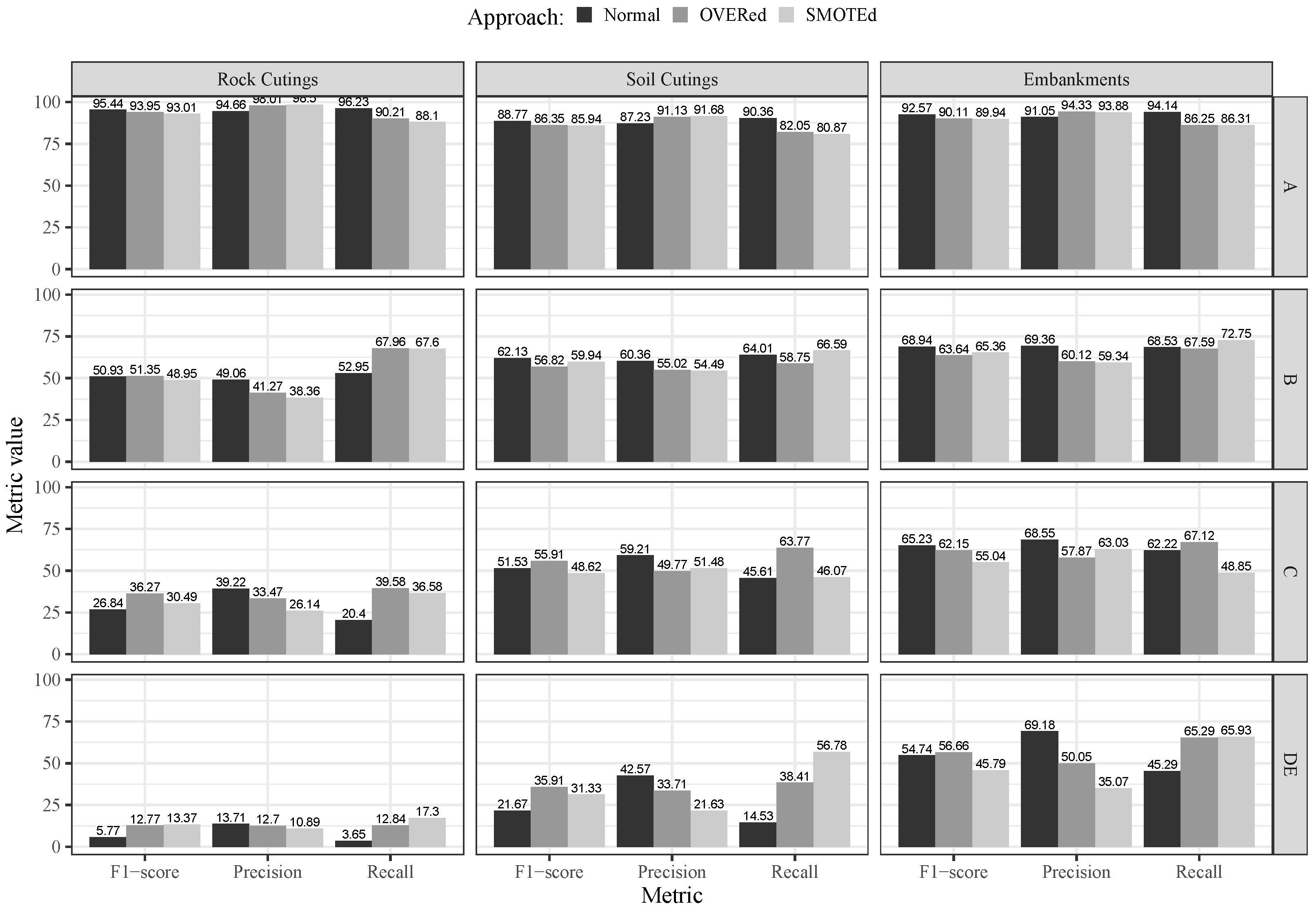
These and numerous other approaches that can be found in the literature, from the perspective of large-scale network management, are constrained to a limited applicability domain and reliant on information that can be difficult and expensive to obtain. In addition, determining whether a slope will fail or not is frequently a difficult task involving many variables and high dimensionality. In order to work around these kinds of restrictions and aid in the decision-making process for large-scale network management, a first endeavor was recently made [30,31] by comparing two popular types of data mining (DM) algorithms: artificial neural betworks (ANNs) [32,33] and support vector machines (SVMs) [34]. When compared with other simpler learning models (e.g., multiple regression or logistic regression models), the ANN and SVM models are more flexible learners, being capable of learning complex input-to-output mappings. We particularly note that the two initial slope stability prediction studies [30,31] assumed a fixed set of selected input variables that could easily be collected during routine inspection activities. The main goal was to compare two learning models (ANN and SVM) for both regression and classification tasks. The preliminary studies [30,31] provided some useful insights that helped to design the approach proposed in this work. Firstly, the best predictive results in both works were produced by the ANN model when performing a nominal classification. Secondly, while interesting predictive results were achieved by the ANN model, the performance was far from ideal. In particular, a high error was obtained for the infrequent EHC (earthwork hazard category) classes (which are related to more hazardous conditions). Thirdly, although the implementation of resampling techniques to handle the imbalanced data issue (which arises as the majority of slopes are in perfect condition) has not always been effective; in some instances, it aided the algorithms in better learning the problem. Such an asymmetric distribution of the data represents a key challenge of the work since it affects the model’s response over all four EHC classes. Fourthly, it was observed that the identification of slope stability is governed by a specific group of characteristics. Figure 1 compares the performance of ANN models when identifying the slope stability of rock and soil cuttings as well as soil embankments based on recall, precision, and ${\mathrm{F}}_{1-\mathrm{score}}$ metrics. More information about the achieved performance can be found in the published works [30,31]. As demonstrated, and taking recall measure as a benchmark, an exceptional prediction ability was observed for class “A”. Class “B” also exhibited strong accuracy. Nevertheless, for classes “C” and “D”, which had a higher probability of failure, the attained performance fell short of expectations, specifically for rock cuttings.

Following the same strategy adopted during the first attempt (i.e., the use of information that can be readily obtained through routine visual inspections [30,31]), the researchers conducted additional tests. In this research, we propose a novel method to improve the performance of models identifying the stability of rock and soil cuttings, as well as embankments. Thus, this paper combines two artificial intelligence (AI) techniques: genetic algorithms (GA), which are popular metaheuristics methods for optimization, and ANNs, which have non-linear learning capabilities. This combination, known as an evolutionary neural network (ENN), allows us to gain interesting capabilities from both AI techniques. In particular, GA is used to perform a search of the best set of input features, which represents one of the major challenges of this work, thus performing automatic feature selection. When compared with other GA input feature optimization works (e.g., [35]), the novelty of our GA approach is that we adopt Pareto curve optimization, allowing us to simultaneously optimize performance measures for all four EHC classes (and not just a single overall performance measure). We note that Pareto curve optimization methods need to keep track of a population of diverse solutions, and GAs are a natural and popular approach for such multi-objective optimization tasks [36]. As for the ANN, it uses a selected set of features as inputs and performs a non-linear mapping with the target output, allowing us to automatically obtain data-driven multi-class classifiers. As underlined above, it is expected that by using a reduced number of features to feed the ANNs, their predictive performance will improve. Finally, a detailed sensitivity analysis was applied to the best ENN models for each one of the three types of slopes, allowing us to identify the key variables in the identification of slope stability.

In conclusion, the primary objective of this study is to develop a simple and rapid method to identify the stability level of a given slope based on visual information that can be readily obtained during routine inspections. However, it is important to note that, from a network management perspective, the use of visual data is enough for the identification of critical network zones, for which additional information can be later collected to conduct a more detailed stability analysis, which is beyond the scope of this study. This innovative approach aims to aid the administrative organizations of railway networks in allocating existing resources to rank assets based on their stability.

2. Data Characterization

As was already indicated, this work combines ANNs and GA with the goal of creating novel models to identify their stability, from this point referred to as EHC [29], of rock and soil cuttings as well as soil embankments.

The EHC system is composed of four levels, “A”, “B”, “C”, and “D”, where the probability of failures increases from class “A” to “D”. Three distinct databases were compiled for training and testing purposes, each containing information gathered during routine inspections and supplemented with geometric, geological, and geographic data for each slope. All three databases were compiled by NetworkRail employees and are related to the UK railway network. On the basis of their experience, NetworkRail engineers attributed a class of the EHC system to each slope, which was taken as a stand-in for the slope’s actual stability conditions for the year 2015.

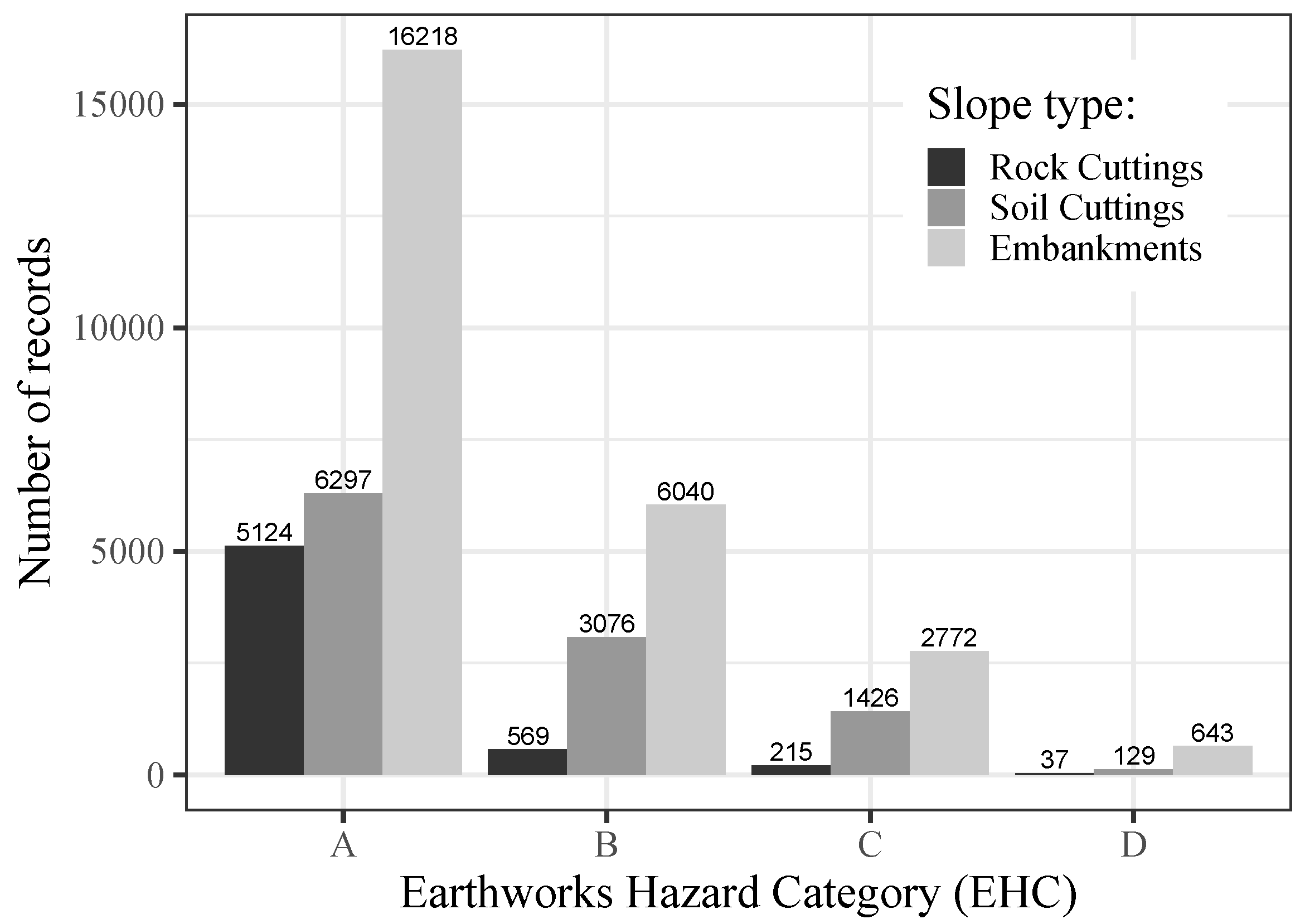
Figure 2 represents the distribution of EHC levels. Its analysis reveals a significant number of available records for all three types of slopes, namely 5945 and 10,928 records for rock and soil cuttings, respectively, and 25,673 records for embankment slopes. We also noted a high asymmetric distribution (imbalanced data) of the records for each EHC class. For example, taking as reference the database for embankments, more than 63% of the data are classified as class “A”, and only 2.5% belongs to class “D”.

Although this type of asymmetric distribution, where the majority of the slopes have a low failure probability (class “A”), is typical and desirable from the perspective of slope network management and slope safety, it can pose a significant learning challenge for DM models. In fact, when dealing with imbalanced classification tasks in which at least one target class label has fewer training samples than other target class labels, the straightforward application of a DM training algorithm frequently results in data-driven models with improved prediction accuracy for the majority classes and decreased classification accuracy for the minority classes. Thus, methods such as oversampling and the synthetic minority oversampling technique (SMOTE), which modify the data to be used for training purposes with the aim of balancing the target class, are frequently adopted to handle datasets where the classes are not equally distributed (imbalanced). In particular, oversampling is a straightforward strategy that balances the final training set by adding random samples (with repetition) of the classes with fewer training data. SMOTE is a more advanced method that generates “new data” by establishing a neighborhood by examining the nearest neighbors and then sampling from that neighborhood. It assumes that the proximity of the original data makes it comparable. By creating synthetic instances, SMOTE helps to increase the representation of the minority class, making the dataset more balanced. This can lead to improved model performance, especially when the class imbalance is significant. It is important to note that SMOTE should be applied only to the training set and not the entire dataset. Also, it is recommended to combine SMOTE with other techniques, such as undersampling the majority class or using more advanced algorithms, such as the SMOTE-ENN (SMOTE with edited nearest neighbors) method, to further enhance the effectiveness of the resampling process. Under the SMOTE approach, regarding the nearest neighbours’ k values, different values were tested before settling on $k=3$, which achieved the highest performance.

More than 50 variables were taken into consideration as model features, including information typically gathered during routine inspections, as well as data from geometric, geographic, and geological sources. To be precise, 65, 51, and 53 variables were considered, respectively, in the study of rock and soil cuttings and embankment slopes. A complete list of all variables considered in each study can be found in Tinoco et al. [31] and Tinoco et al. [30].

3. Methodology

3.1. Artificial Neural Networks

As shown above in Figure 1, which illustrates the models’ performance in EHC prediction that was achieved during the first experiments [30,31], the ANN algorithms produced the most effective overall results. Accordingly, only ANNs were trained for EHC prediction in this new attempt.

It should be noted that ANNs are among the most effective DM algorithms for resolving challenging issues across a variety of knowledge domains [37,38,39], including in civil engineering [40,41,42,43]. In slope stability problems, several applications of ANNs can be found in the literature [13,44,45]. Another important point of evidence underlying the huge potential of ANNs is their recent developments under the deep learning field, which have significantly advanced the state of the art in speech recognition, visual object recognition, object detection, and numerous other fields, including drug discovery and genomics [46,47,48].

In spite of these important advances, in this work, we adopt the “traditional” neural networks. In a nutshell, ANNs are learning systems that originally were driven by how human brains work [49]. They process information iteratively by multiple neurons. ANNs are reliable when exploring data with noise and are capable of modeling intricate non-linear mappings. This research adopted the following parameters for the ANN:

• A multilayer perceptron with only feedforward connections;
• One hidden layer containing H processing units;
• A grid search of $\{0,2,4,6,8\}$ to determine the optimal value of H;
• A logistic function applied to the neural function of the hidden nodes $1/(1+e^{-x})$;
• The BFGS technique [50] as an optimizer for the ANN.

The BFGS technique is a quasi-Newton method (also referred to as a variable metric algorithm) that was published simultaneously in 1970 by Broyden, Fletcher, Goldfarb, and Shanno [50]. It uses function values and gradients to construct a representation of the optimized surface [51].

3.2. Genetic Algorithms

In a data-driven undertaking, it is common practice to employ heuristic search methods, such as GA [52], for feature selection. In fact, when compared to exhaustive search methods, which can become computationally intensive for larger datasets [52], iterative algorithms such as sequential search or evolutionary algorithms (e.g., GA) [53] are more likely to produce interesting optimization outcomes with a moderate use of computational resources.

As stated in Section 2, models can be fed with a substantial number of input features (more than 50 variables). Feeding all of these attribute features to the learning models will increase the model’s complexity and decrease the accuracy of its predictions, as some of these features may not be particularly relevant. However, the search space for all possible input combinations is excessively large ($2^{50}$). Thus, we employed a GA in this study to identify the optimal set of input features that improve EHC prediction. These modern and versatile optimization techniques stand out as some of the most potent optimization tools due to their ability to handle large search spaces with minimal computational overhead and their simplicity of interpretation and application.

Supported by AI and natural selection, a GA starts by coming up with random answers to a problem, which are then improved step by step until they are optimal or close to optimal. Based on that, the GA [53] can be used to determine the subset of features [54,55] where the bits on the chromosome show whether or not the feature is present. Finding the global maximum for the objective function will yield the finest suboptimal subset. In this case, the objective function is the predictor’s performance.

GAs can do more than just optimize a single goal. This is very important because there is often not a single best trade-off answer, but a set of trade-offs with different goals. When addressing slope stability assessments, the capability to predict well in all four classes of the EHC classification system, and not in just one, is of the utmost importance. Due to the asymmetrical distribution of the data, which could result in a high overall performance based solely on a high level of accuracy for class “A” (the most common class), this characteristic is of the utmost importance.

Consequently, for multi-criteria optimization tasks, optimizing a Pareto front of solutions is one of the most effective strategies. Thus, each solution is deemed non-dominated, or Pareto optimal, if none of the objectives can be improved in value without deteriorating the others [56]. In the context of slope management, all Pareto optimal solutions can be assumed to be equivalent, and the decision maker or project manager can establish the primary selection criteria for choosing one solution over another based on the characteristics of the via (e.g., urban or rural location) through which a network of slopes is connected.

Since Pareto front multi-optimization requires keeping an eye on a population of solutions, population-based meta-heuristics, such as evolutionary multi-objective optimization (EMO), have become common solutions. Evolutionary computational methods, such as GA and EMO, operate by sustaining a population of individuals (potential solutions), where a chromosome represents an individual data representation of a solution and a gene represents a value position within such a representation. The design of the chromosome is a crucial aspect of adopting evolutionary approaches, as it defines the problem’s search space. In this research, each chromosome is a sequence of 1 and 0 genes, with each gene indicating whether a characteristic is present (1) or absent (0).

This study implements a well-known EMO search engine, the non-dominated sorting genetic algorithm-II (NSGA-II [57], to address the slope stabilization identification multi-criteria optimization problem. The NSGA-II algorithm was adopted due to two major factors. Firstly, NSGA-II is a popular and state-of-the-art multi-objective evolutionary algorithm (MOEA) method that tends to obtain state-of-the-art results when the number of objectives is lower than 5. For instance, in [36], the NSGA-II algorithm outperformed other multi-objective methods such as S metric selection (SMS-EMOA) and aspiration set (AS-EMOA). Second, R software allows NSGA-II to be implemented with low computational effort [58] by taking advantage of the mco [59] package.

For NSGA-II parameterization, the standard values as defined in the R software were adopted, as follows:

• Population size: 100;
• Stop criteria: after 100 generations;
• Crossover probability: 0.7;
• Mutation probability: 0.2.

The default parameterization was selected for two main reasons. First, a single run of the hybrid NSGA-II and ANN combination is computationally costly. For instance, under the default parameterization, each GA generation requires the training of 100 ANNs, each trained with thousands of data records. Thus, tuning all NGSA-II hyperparameters (e.g., via grid search [60,61,62]) would require a prohibitive computational effort. Secondly, NSGA-II works as a second-order optimization procedure since it it selects the input variables that feed the ANN training algorithm (the first-order optimization method). Thus, the tuning of NSGA-II’s internal parameters is not a critical issue. In preliminary tests, smaller population sizes (i.e., 20, 30, and 50) and various values for crossover and mutation probabilities were examined. However, the obtained results were inferior to the default values. As the mco package of the R tool employs a real-value representation of the NSGA-II method, all genes were initially rounded to the nearest integer (1 or 0) for the initial fitness function step.

The optimization was executed on a Linux server machine with an Intel Xeon 2.27 GHz. The total computational effort for the optimization depended significantly of the size of the database, but was never below than 672 h (around one month).

3.3. Model Evaluation

When handling unbalanced multi-class datasets (such as our EHC case), single classification measures can result in misleading predicted values. For instance, if there are four classes, “A”, “B”, “C”, and “D”, where 95% of the examples are related to class “A”, then a classifier with a 95% classification accuracy might correspond to a “dumb” predictor that always outputs the “A” class. Thus, in this work, rather than assuming a single measure, we computed performance measures for all four EHC classes.

When evaluating the prediction quality for a particular class, there are two types of errors, false positives and false negatives, each of which correspond to different costs (specific to the domain problem). In order to better measure the prediction performance for each of the four EHC classes, rather than focusing on one type of error (e.g., just false positives), we computed classification metrics that are widely used in multi-class tasks and that consider both types of errors [63]:

• Recall;
• Precision;
• ${\mathrm{F}}_{1-\mathrm{score}}$.

The first measure takes into account false negatives, the second one considers false positives, and the third score provides a trade-off between both measures. The recall, also known as the true-positive rate or sensitivity, assesses the proportion of instances of a particular class that the model correctly identified. In other words, the recall of a certain class is given by the formula $TruePositives/(TruePositives+FalseNegatives)$. The precision metric, also known as the positive predictive value, measures the accuracy of the model when it predicts a particular class. Specifically, the precision of a particular class is determined by the formula $TruePositives/(TruePositives+FalsePositives)$. We further note that there is another measure that considers false positives, the false-positive rate. However, using precision or the false-positive rate would essentially lead to the same quality measurement (i.e., assess the value of false positives). Thus, in this work, we opted to use recall since it is commonly used as a complementary measure that is associated with precision. As for the third measure, the ${\mathrm{F}}_{1-\mathrm{score}}$ corresponds to the harmonic mean of precision and recall according to the following expression: $2·(precision·recall)/(precision+recall)$. All three metrics can range from 0% to 100%, with a higher value indicating a more accurate predictor.

The generalization capability of the ANN models was evaluated using a 5-fold cross-validation method with 5 runs [64], with the exception of the optimization phase, in which a 3-fold cross-validation method with 2 runs was used. This means that each modelling setup was trained $3\times 5=15$ (optimization step) or $5\times 5=25$ (modelling step) times. When compared with the simpler holdout method (single split between training and testing), the k-fold cross-validation procedure has the advantage of obtaining predictions for all the data. Under this approach, the data are randomly split into k mutually exclusive subsets with the same length. Then, a cycle with k iterations is executed, where all data except a differently selected fold are used for training. Once the model is trained, predictions are performed for the selected fold (unseen data). In the end, a total of k models are trained and tested. Thus, the measured performance measures on unseen data are more robust. The k-fold cross-validation procedure ensured that all three prediction metrics (recall, prediction, and ${\mathrm{F}}_{1-\mathrm{score}}$) were always computed on the unseen test data.

3.4. Sensitivity Analysis

A model’s interpretability is of paramount importance, particularly from an engineering point of view, to obtain a detailed understanding of what has been learned by the models. Indeed, data-driven models, namely those based on ANN algorithm, are usually designed as black box models. Explainable artificial intelligence (xAI) [65,66] is a well-established domain with a thriving community that has developed a number of highly effective methods to explain and interpret the predictions of complex machine learning models, such as deep neural networks. In this study, a comprehensive sensitivity analysis (SA) [67] was conducted on the final models (i.e., the Pareto optimal solutions). SA is a simple method that was implemented following the training phase and measured the model’s responses when a given input was modified, thereby allowing one to quantify the relative importance of each attribute.

The SA approach is inspired by experimental design [68], which is often used to identify causal relationships. There are other approaches to obtain knowledge from trained ANNs, such as the extraction of rules from trained ANNs. However, such approaches tend to discretize or simplify the predictive model’s responses, leading to rules that do not accurately represent the original model or that consider just single-input interactions. The advantage of the SA approach is that it accurately measures the trained ANN’s responses (even if the class decision boundaries are complex) under a computationally efficient mapping approach. In effect, and in accordance with the findings of Cortez and Embrechts [69], in this research, we employed a global sensitivity analysis (GSA) technique that is capable of detecting interactions among all combinations of input attributes. In this context, F inputs are changed at same time. F can range from one, as in a one-dimensional SA, denoted as 1-D, to I, as in an I-D SA. Iteratively, each input assume different values withing its range by L levels. The other inputs are held constant at the baseline, b. Seven levels ($L=7$) were adopted in this research, which allowed an interesting amount of detail to be added at a reasonable computational effort. For the baseline b, the average value of each input was considered.

In short, the ANN was initially calibrated to the entire dataset. The fitted model was then subjected to the GSA algorithm, and the respective sensitivity responses were stored. Next, significant visualization techniques were computed using these responses. Specifically, the input importance bar graph illustrates the relative impact of each input variable (from 0% to 100%). The rationale behind SA is that the input is more significant the greater the changes observed in the output. Following the recommendation of Cortez and Embrechts [69], the gradient metric was chosen to measure this effect:

$$g_a={\displaystyle \sum }_{j=2}^L|{\widehat{y}}_{a,j}-{\widehat{y}}_{a,j-1}|/\left(L-1\right)$$

(1)

where a denotes the input variable under analysis and ${\widehat{y}}_{a,j}$ is the sensitivity response for $x_{a,j}$. We note that in [69], other SA measures were tested, including range and variance. However, in that study, it was shown that the gradient measure is more theoretically sound and provided better experimental evidence when compared with the range and variance measures (e.g., the variance tended to overemphasize the importance of the most relevant input, while the range provided an identical value for linear or high-frequency wave responses that produced the same range). Having computed the gradient for all inputs, the relative importance ($R_a$) was then calculated using:

$$R_a=g_a/{\displaystyle \sum }_{i=1}^I{g}_i·100(\%)$$

(2)

3.5. Modelling Procedure

A nominal classification approach showed the highest overall response on EHC prediction during the first attempt [30,31]. Accordingly, the same modelling strategy was adopted in this new attempt. In addition, as mentioned before, only ANN algorithms were trained, as they showed superior performance in the EHC problem. SMOTE, oversampling, and no resampling were also tested in these new experiments (only during the modelling step) in order to address the issue of imbalanced data [70,71], as no conclusive conclusion could be drawn from the first attempt regarding the optimal resampling technique. We note that the three resampling approaches are reasonably diverse. The no resampling option did not change the training data; thus, it was used as a baseline to check if the other resampling approaches provided a modelling value. Since the minority classes occurred very infrequently, it made more sense to apply oversampling rather than undersampling (if this last method was applied, the training data would be too small). Finally, SMOTE is a state-of-the-art resampling technique that generates synthetic samples for minority classes.

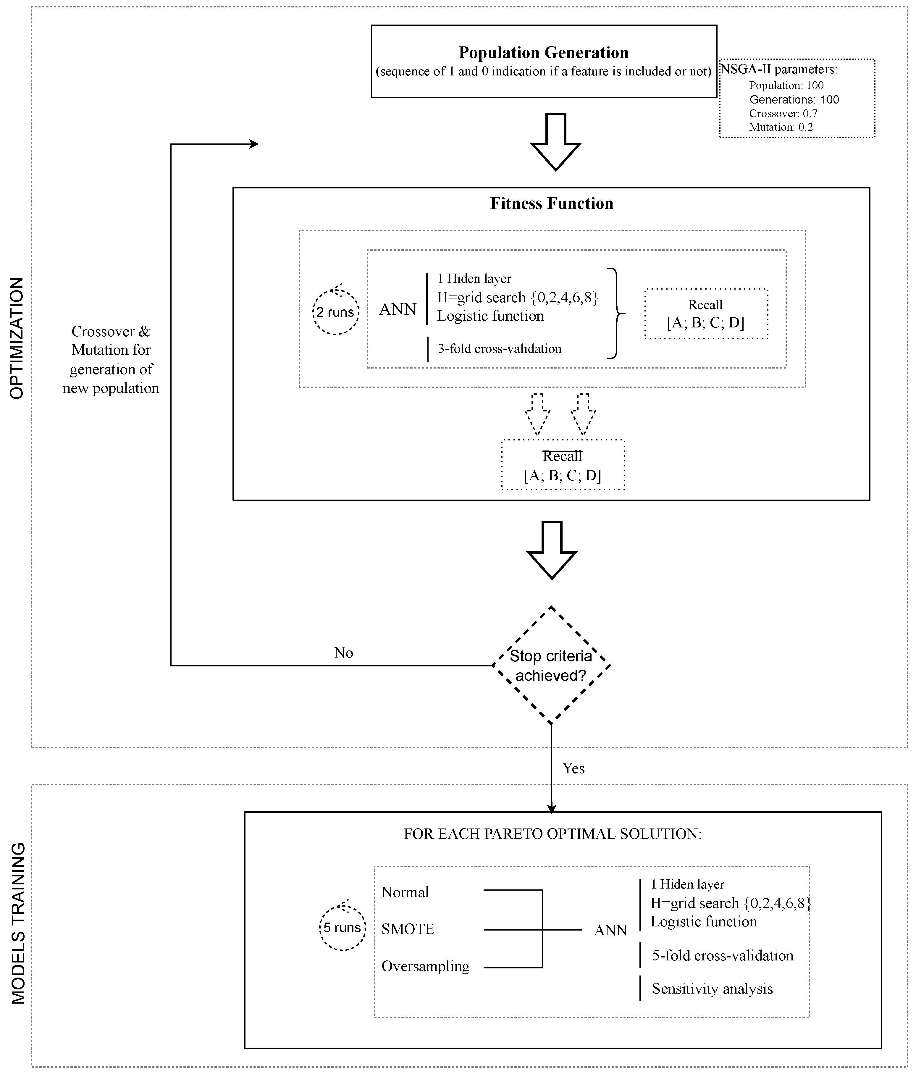
The overall proposed procedure was comprised of two main steps, as illustrated in Figure 3 and as described below:

• Optimization: The objective of applying GA is to identify the optimal set of variables that minimizes the objective function. Consequently, our GA began by randomly defining an initial population in which each individual (a sequence of 1 and 0 indicating whether a feature was included or not) represented a potential solution (set of variables) to the problem. The objective function corresponded to the maximization of the recall metric for all four EHC classes (a multi-objective problem). The fitness function corresponded to an ANN algorithm-based predictive model. Two ANNs were fitted to the database using the methodology outlined in Section 3.1 (i.e., a feedforward network with one hidden layer, a logistic function for hidden nodes, and a grid search of $\{0,2,4,6,8\}$ for H definition using a 3-fold cross-validation schema as the validation procedure). Then, for each EHC class, a recall metric (the average of both ANNs) was calculated, which was then utilized by the GA to optimize the optimal set of attributes for EHC identification.
• ANN training: After optimization, five ANNs were fitted to the database for each Pareto optimal solution (set of optimal variables) using the methodology described in Section 3.1. Here, in addition to the standard approach (no resampling), ANNs were trained with a resampled database using the SMOTE and oversampling approaches. Notably, the various sampling methods were only applied to the training data, which were used to fit the data-driven models, and the test data (as provided by the 5-fold cross-validation procedure) were not altered. This means that $3\times (5\times 5)=75$ ANNs were trained for each Pareto optimal solution. Each model was then subjected to a sensitivity analysis to determine the relative relevance of each attribute for EHC prediction.

As presented and discussed in the next sections, it was possible to identify the average number of input variables considered for EHC prediction. In addition, the variables selected more frequently by the GA were determined. In the end, based on the overall performance of each model (measured by the recall, precision, and ${\mathrm{F}}_{1-\mathrm{score}}$ for all four EHC classes) and the results of the sensitivity analysis, a single model was chosen and thoroughly analyzed.

Although not presented in the paper, it should be mentioned that some other experiments were also carried out following a regression strategy, where, in addition to the optimization of the best set of attributes, a numeric regression scale was also optimized at the same time.

The R statistical environment [58] was adopted to implement all experiments conducted in this research. Moreover, to facilitate the implementation of ANNs and NSGA-II algorithms, as well as validation techniques such as cross-validation, the rminer [51] and mco [59] packages were used.

4. Results and Discussion

This section summarizes the main achievement in the EHC prediction of rock and soil cuttings from slopes and embankments by combining the learning capabilities of the ANN and the optimization power of the GA.

4.1. Feature Selection

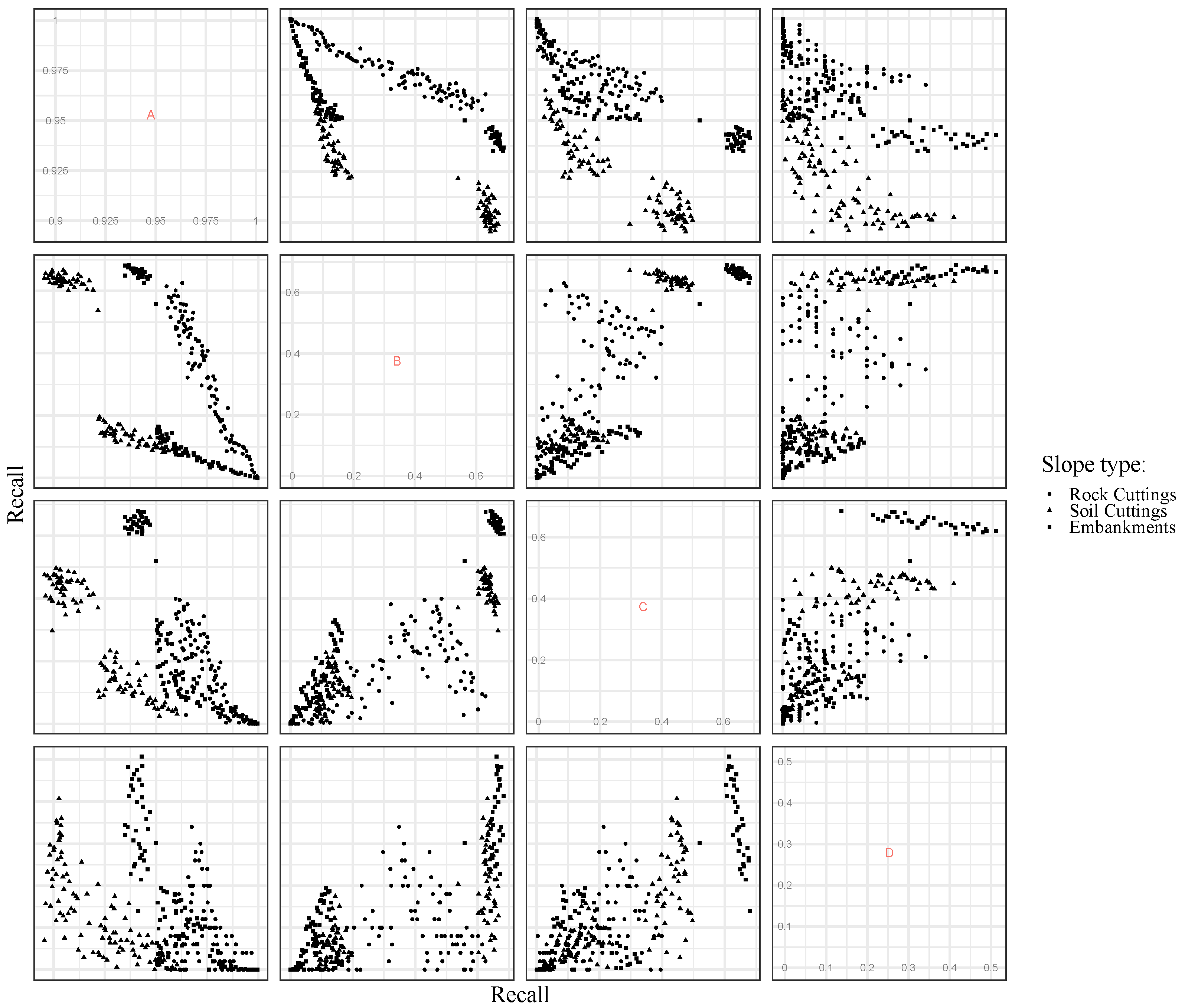
Figure 4 depicts the trade-off between recall values for each one of the four EHC class for all Pareto optimal solutions covering the three case studies, that is, rock and soil cuttings and embankments. Although putting all this information in a single graph is somewhat confusing, for the purposes of analysis, itis more than enough, as it aims at providing an overview of the performance for each EHC class.

From its analysis, and as expected, the best solution is always a performance commitment between all EHC classes. This commitment is particularly evident between class “A” and classes “B”, “C”, and “D”. For example, to obtain a high performance for class “A”, the response for the other classes must be compromised in some way. The same behavior is also observed for the other possible EHC class combinations, although in some instances, specifically between the “B” and “C” classes, commitment is not as evident. In fact, there are some solutions that maximise the response for such classes. In addition to the performance commitment between EHC classes, Figure 4 also demonstrates the inferior performance of all Pareto optimal solutions for classes “C” and “D”, namely for rock cuttings (below 0.4) when compared to class “A” (above 0.9).

As previously stated, GAs were applied in this study for feature selection purposes; in other words, they were used to find the best model (set of input variables) that maximized EHC prediction. However, some additional and useful information was extracted from the achieved results, which was useful to obtain a better understanding of the behavior of the stability of slopes. Specifically, they provided information regarding the optimal number of inputs for the accurate determination of slope stability, as well as the variables that should be used as model attributes.

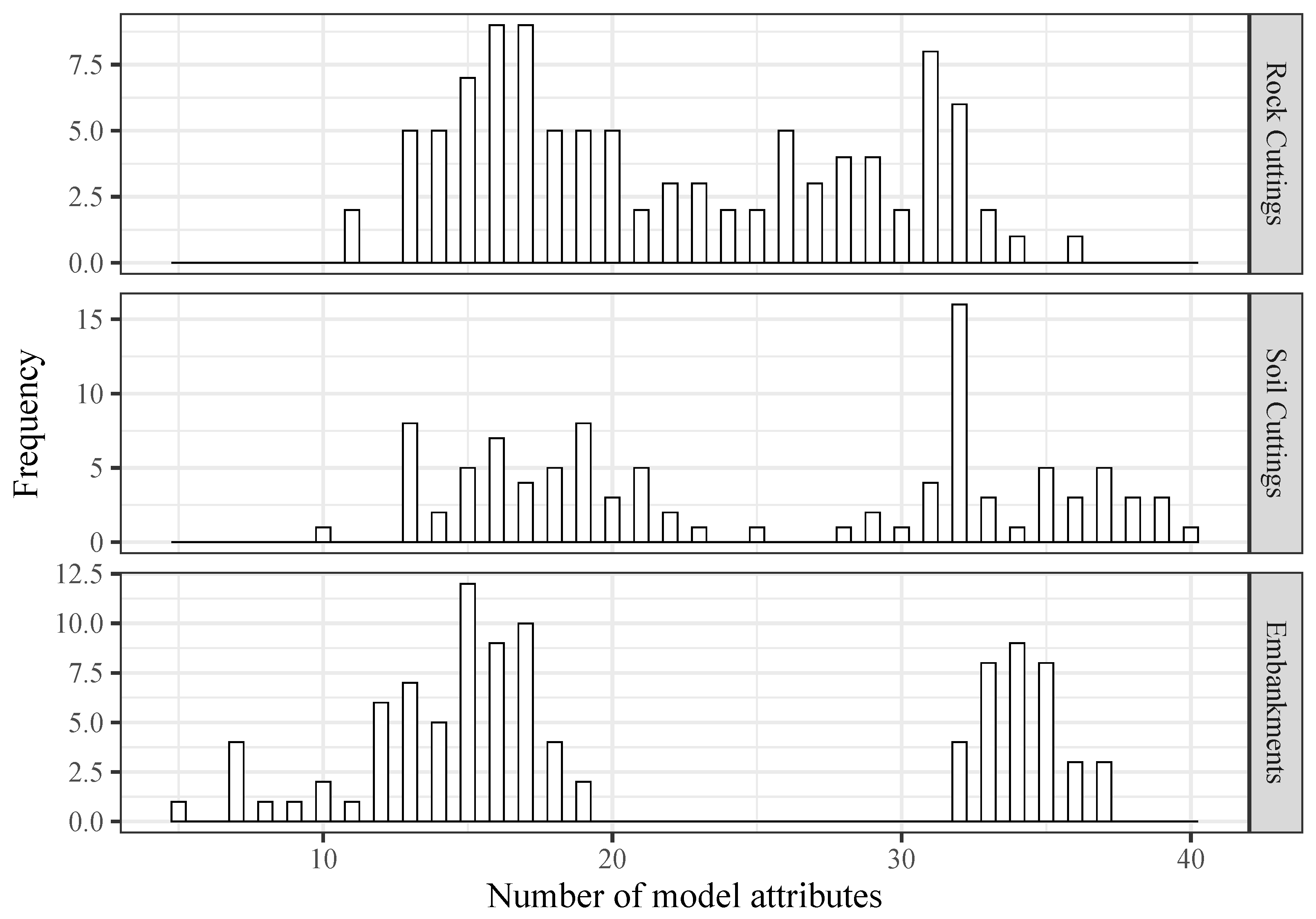
Figure 5 demonstrates that, with the exception of embankments, all Pareto optimal solutions evaluated fewer than ten features and no more than forty inputs. There are some solutions for embankments that considered fewer than ten inputs, with a minimum of five attributes. Still, in regards to embankments, it is interesting to observe that most of the solutions have considered, on average, 15 or 34 inputs. Moreover, for the rock and soil cuttings’ slopes, although this was not so evident, the number of variables considered by a significant part of the solutions ranged between 10 and 20 or between 30 and 40. These observations indicate that only about half of the more than 50 features available for model training were simultaneously considered as input to a model. In fact, the majority of Pareto optimal solutions in the study of rock cuttings considered between sixteen and seventeen features, while some were fed by as many as thirty-one features. Regarding soil cutting, the most frequent number of variables taken by the Pareto optimal solutions was 12, and for embankments, that number was 15.

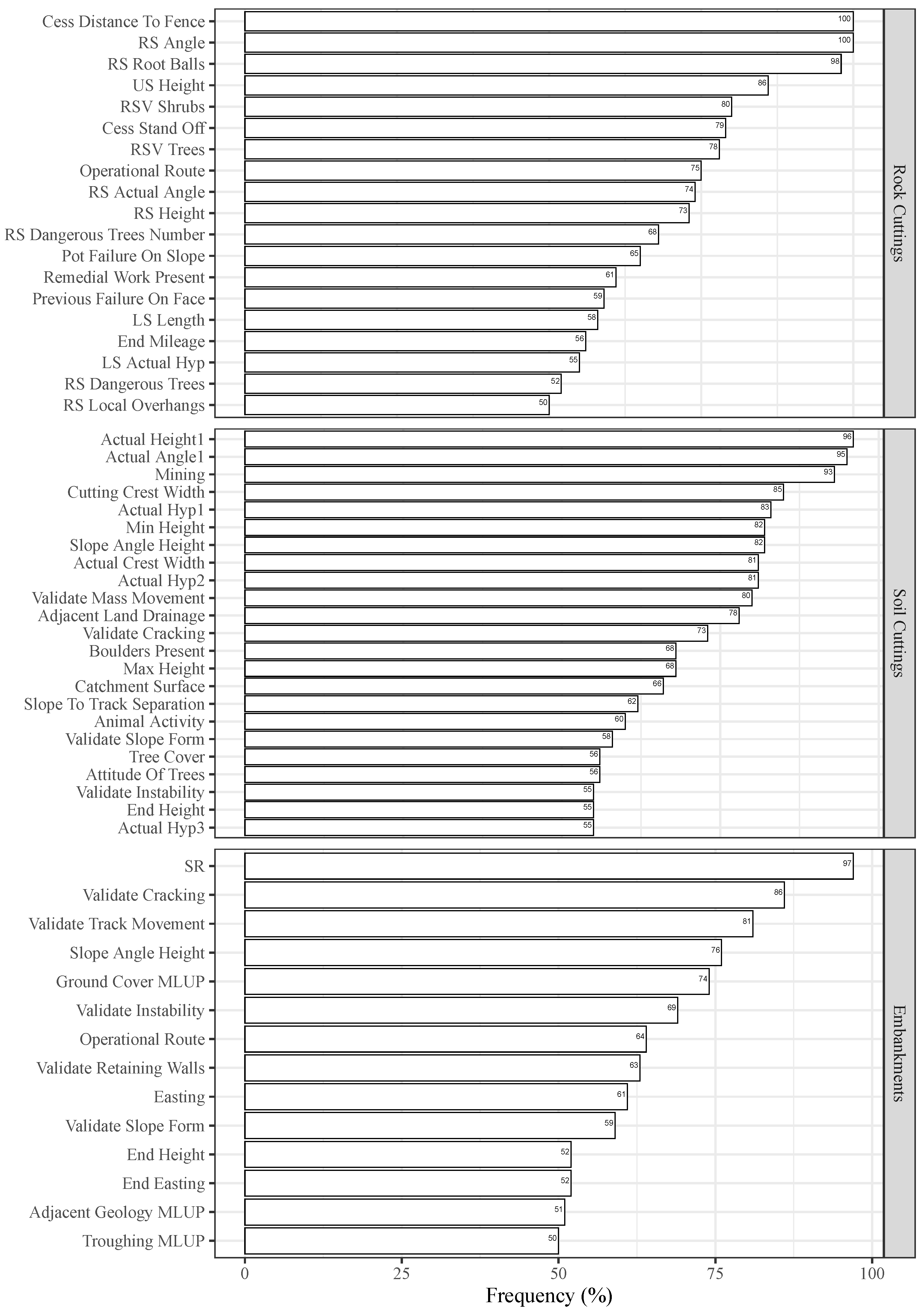
From Figure 6, which shows the variables present in at least half of all Pareto optimal solutions, it can be observed that slopes categorized as “high” and “angle” are common to the three types of slopes. Moreover, it can also be observed that only three variables were considered as model attributes by all Pareto optimal solutions among the three slope types. Comparing the three slope types, higher variability was observed for embankments in terms of the model attributes considered by any Pareto optimal solution. In fact, only a restricted group of 14 variables are present on 50% of all Pareto optimal solutions. When considering rock and soil cuttings, this number becomes almost twice higher, particularly for soil cuttings, where a group of 23 variables were used by 50% of all solutions.

4.2. Model Performance

A single model was chosen from all Pareto optimal solutions for aeach slope type on the basis of the recall, precision, and ${\mathrm{F}}_{1-\mathrm{score}}$ performance metrics across all EHC classes. As summarized in Section 3.5, all Pareto optimal solutions were retrained using the SMOTE and oversampling techniques, as well as without resampling (normal). The efficacy of these Pareto optimal solutions for each slope type is presented and discussed in the following sections.

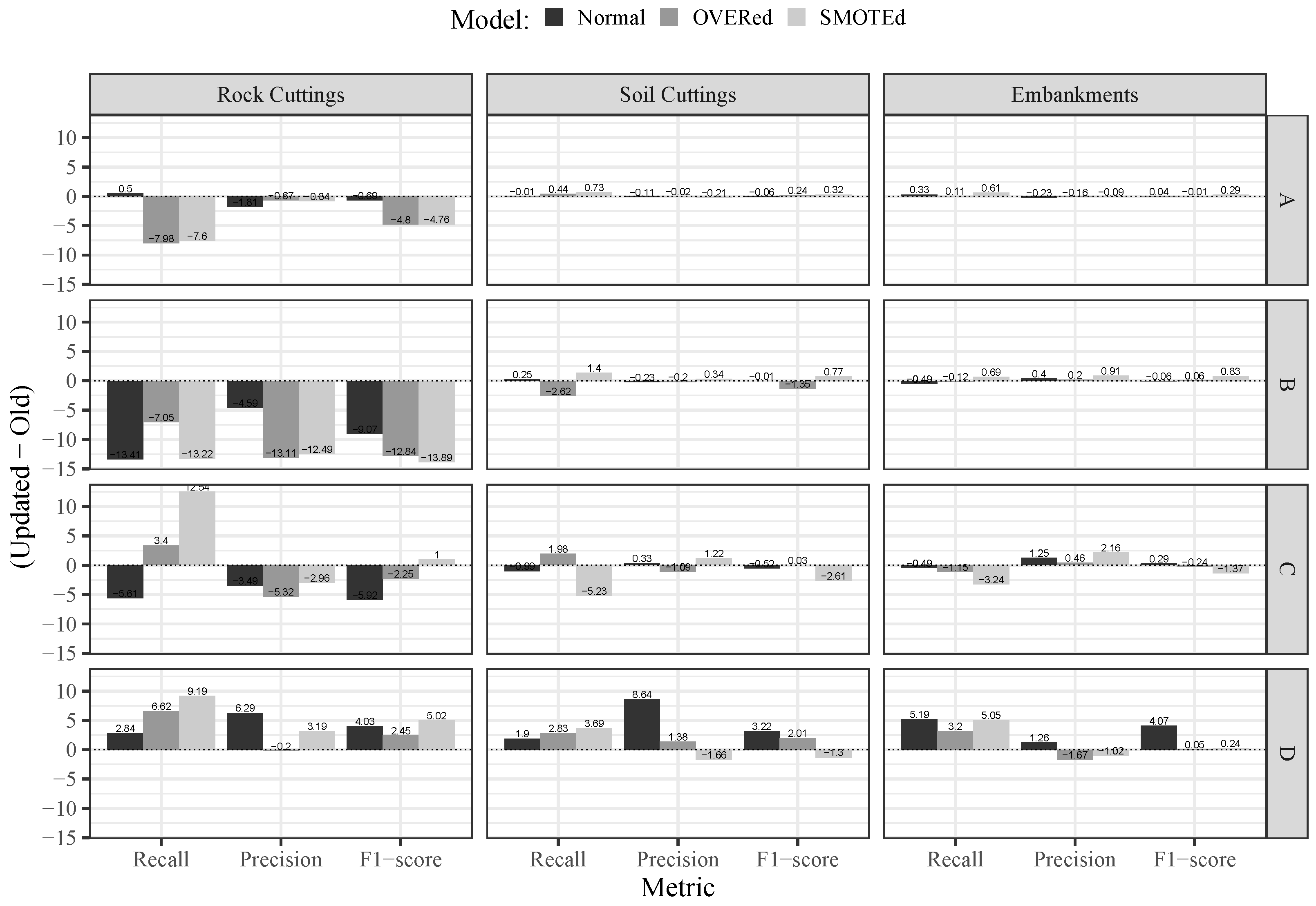
Using the recall, precision, and ${\mathrm{F}}_{1-\mathrm{score}}$ metrics as benchmarks, Figure 7 compares ANNs models from the first ANN models (from now referred to as the “old” models [30,31]) and the best ANN models selected among all Pareto optimal solutions (referred to from now on as the “updated” models). This comparison was made by calculating the difference between the metrics of the “updated” and “old” models. Hence, positive values correspond to the superior performance of the “updated” models. Despite the fact that the overall difference between the “updated” and “old” models is not statistically significant, the “updated” models have several key advantages over the “old” ones. On the one hand, using the recall metric as a benchmark, the “Updated” models, particularly those following a SMOTE approach, demonstrate a significant improvement in the prediction of classes “C” and “D”. On the other hand, this “updated” model utilizes a significantly reduced number of features. On average, less than 30 variables were considered instead of the more than 50 considered in the “Old” models. These two aspects represent a significant accomplishment from a practical standpoint. First, less information is required to accomplish the same overall performance, which represents significant time and cost savings. Second, a better performance on classes “C” and “D” prediction was achieved with almost no performance penalization for the remaining classes.

This trade-off between the models’ responses for the major and minority classes is a consequence of the highly asymmetric distribution of the database. However, it should be noted that the “updated” models achieved a better balance by increasing their performance for the minority classes, for which the probability of failure is higher, without significantly compromising their responses for the major classes.

When analyzing the effect of the training sampling approaches (oversampling and SMOTE), some effectiveness can be observed for classes “C” and “D”, for which the probability of failure is higher (as these are minority classes), particularly for rock cuttings. Concerning classes “A” and “B”, the implementation of a sampling approach does not produce the same effectiveness. When comparing SMOTE and oversampling, the effectiveness of the first method seems to be slightly superior. These results are in line with those observed during the first iteration, as reported in [30,31].

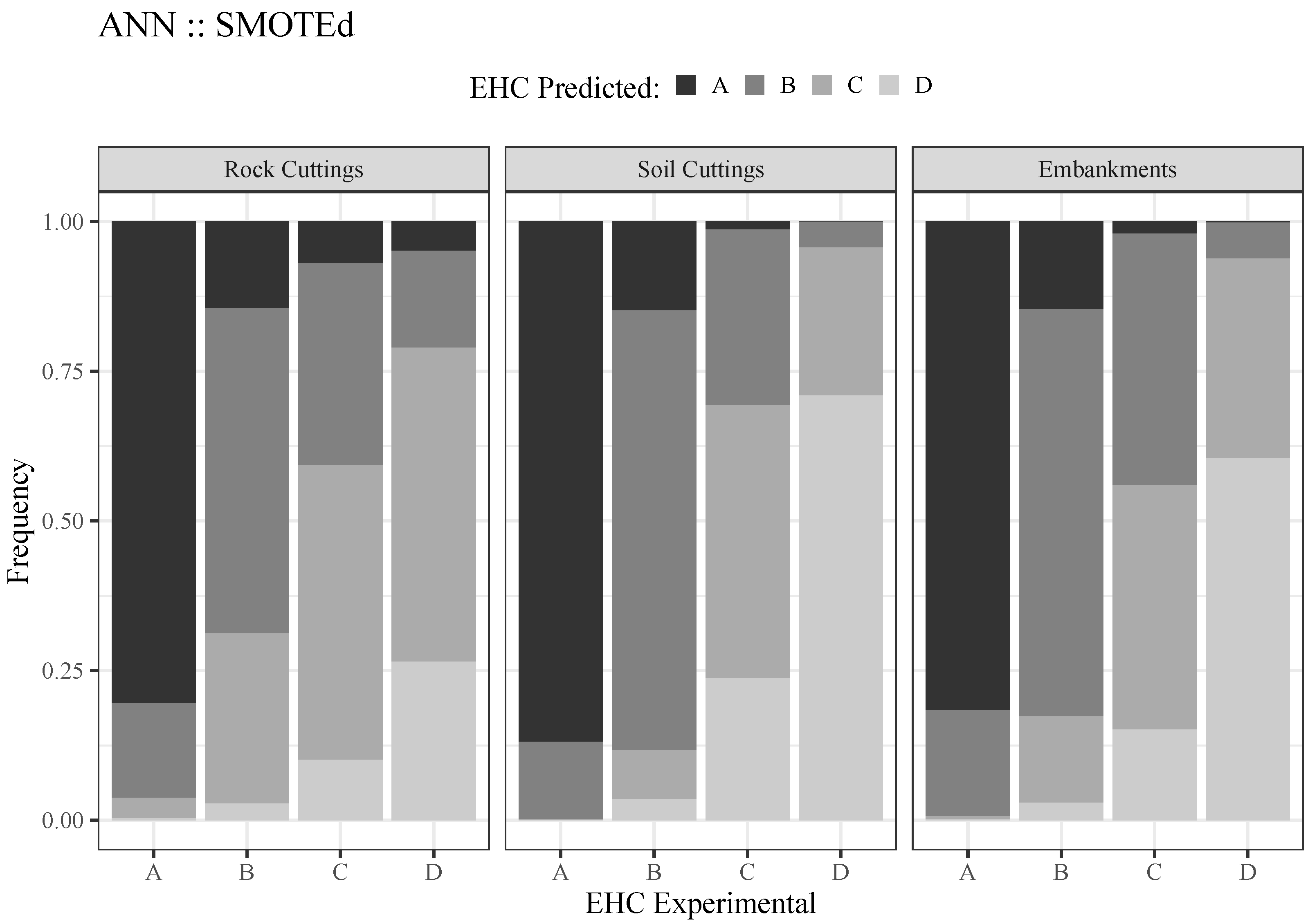
Figure 8 depicts the relationship between the observed and predicted EHC classes based on the “updated” SMOTE-based ANN model. Its superior performance on classes “A” and “B” is evident from its analysis. Particularly for soil cuttings and embankments, we can also observe a very interesting response for class “D” (more than 60% of the slopes belonging to class “D” were correctly identified). Furthermore, one can observe that when a slope’s class is not correctly identified, it is categorized as belonging to the closest class. For instance, a slope of class “D” that is not predicted as “D” is typically classified as “C”. These results are encouraging and drive new experiences toward improvements in the performance of models, particularly for minority classes.

4.3. Model Interpretation

As important as the performance of a model is, its interpretability is also highly important, particularly when it is based on complex algorithms, such as ANNs. Due to their mathematical complexity, these models are typically difficult to understand and usually referred to as “black boxes”. Therefore, it is essential to “open” such models in order to comprehend what they have learned. In this study, a GSA methodology [67] was used to identify the most important parameters (1-D SA, input importance bar plot).

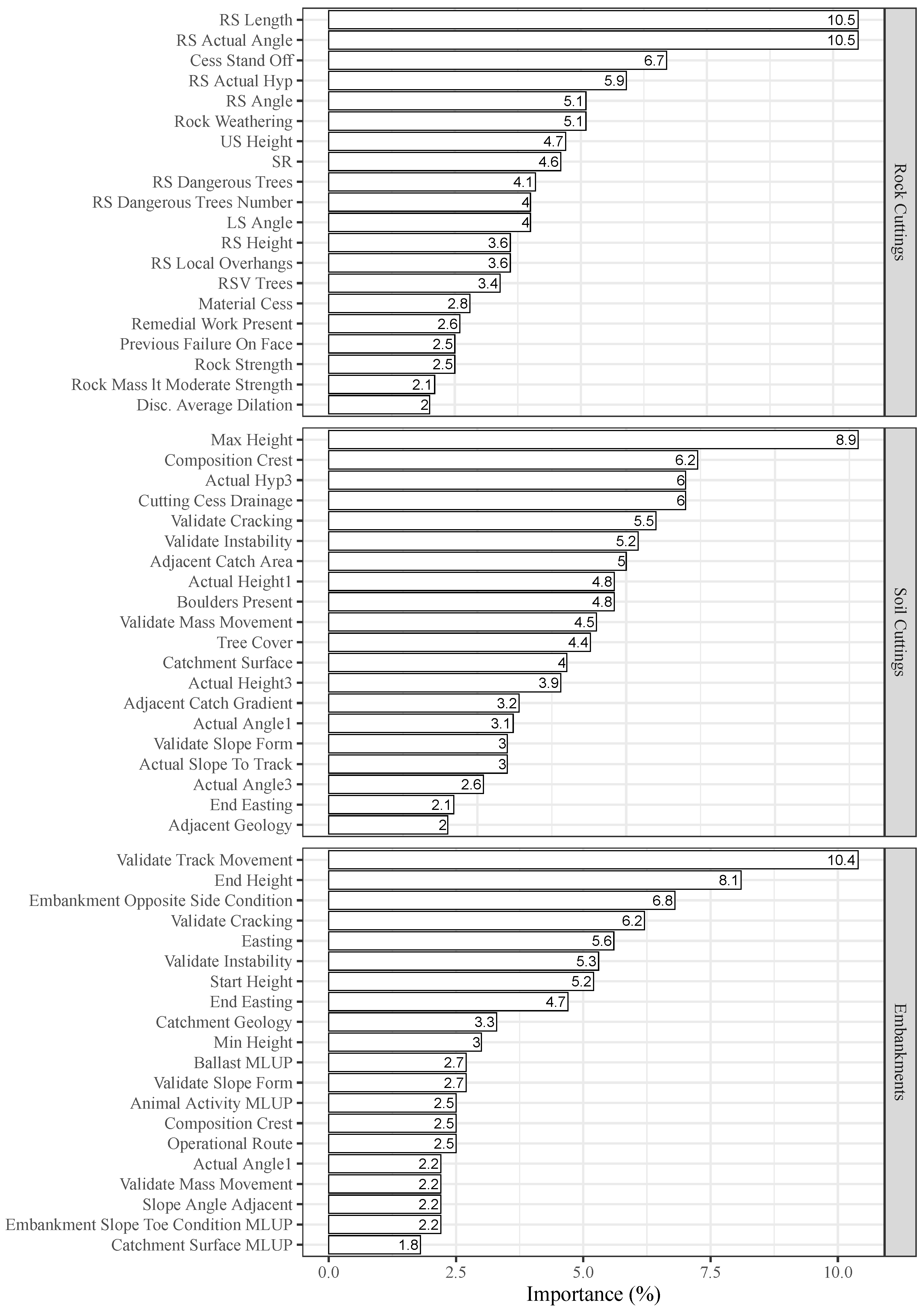
Figure 9 shows the relative importance of the twenty more relevant variables according to the best “updated” models, as described above.

Comparing this ranking with the “old” models reported on [30,31], it can be observed that both rankings share around half of the more relevant features. The exceptions are the rock cuttings, where only 6 of the 20 more relevant variables were also identified as such in the “updated” models.

Focusing only on the 20 more relevant variables according to the “updated” models for each of the slope types, it can be observed that any variable has an individual influence higher than 10.5 %. Concerning the rock cuttings, the variables “RS Length” and “RS Actual Angle” present a relative importance of 10.5%. In the case of soil cuttings, the variable “Max Height” stands out from the others, with an influence of 8.9%. Relating to embankments, the variable “Validate Track Movement” presents a relative influence of 10.4%, which is closely followed by “End Height”, with 8.1%. Moreover, it can also be observed that at least one variable related to the slope angle or slope height appears at the top of the ranking.

Overall, these rankings follow what is known regarding the main factors relating to slope stability [2,15,20,21,27]. Several empirical studies have shown that a high slope and its angle are among the key factors that mostly contribute to the stability of a given slope [1,14,22,28].

5. Final Remarks

After a first attempt to identify the stability of rock and soil cuttings and embankments using machine learning algorithms and taking into account the visual features that are usually collected during routine inspections, a second attempt was made by combining artificial neural networks (ANNs) and genetic algorithms (GA), a combination also known as an evolutionary neural network (ENNs), for feature selection and slope stability classification purposes. This innovative approach allows ANNs and GAs to work together to assess the stability of a slope. Although the overall performance did not improve significantly, the new models presented some important advantages. First, to achieve the same overall performance, the number of input variables decreased to less than 30. This is a key point from a practical point of view since it endows the model with more flexibility when less information is available. Furthermore, this can allow the railway infrastructure management companies to collect less information to determine the stability level of their slope network, which, in turn, will allow them to reduce costs related to routine inspections. Second, better performance is achieved for the identification of classes “C” and “D”, which correspond to a higher probability of failure, without significantly compromising the model’s performance on the remaining classes. From a safety point of view, this represents a significant improvement, allowing for the strategic investment of the available budget on critical slopes. In addition, such a strategic maintenance plan can reduce traffic constraints due to slope failures and, consequently, the probability of severe incidents. In summary, these results are encouraging and consist of a promising research direction towards a more efficient identification of the stability of slopes, particularly for minority classes. Thus, as a future development, we intend to explore other feature selection approaches as well as different strategies to handle imbalanced data (e.g., the usage of Tomek links or Gaussian copula transformations [72]). In addition, considering the high number of data available for each of the three slope types, a deep learning approach may provide an important contribution toward the prediction models’ efficiency.

Despite the fact that new attempts are still necessary, this study demonstrates once more the extreme difficulty of such a task, namely by considering only visual features. Nonetheless, this difficult task is of the utmost importance, especially for developed nations that must maintain large-scale transportation networks despite limited budgets for maintenance and network operations.

References

- Pourkhosravani, A.; Kalantari, B. A Review of Current Methods for Slope Stability Evaluation. Electron. J. Geotech. Eng. 2011, 16, 1245–1254. [Google Scholar]
- Ullaha, S.; Khanb, M.U.; Rehmana, G. A Brief Review of the Slope Stability Analysis Methods. Geol. Behav. 2020, 4, 61–65. [Google Scholar]
- Suchomel, R.; Mašı, D. Comparison of different probabilistic methods for predicting stability of a slope in spatially variable soil. Comput. Geotech. 2010, 37, 132–140. [Google Scholar] [CrossRef]
- Sivakumar Babu, G.; Murthy, D. Reliability analysis of unsaturated soil slopes. J. Geotech. Geoenviron. Eng. 2005, 131, 1423–1428. [Google Scholar] [CrossRef]
- Husein Malkawi, A.I.; Hassan, W.F.; Abdulla, F.A. Uncertainty and reliability analysis applied to slope stability. Struct. Saf. 2000, 22, 161–187. [Google Scholar] [CrossRef]
- Gavin, K.; Xue, J. Use of a genetic algorithm to perform reliability analysis of unsaturated soil slopes. Geotechnique 2009, 59, 545–549. [Google Scholar] [CrossRef]
- Wang, H.; Sassa, K. Comparative evaluation of landslide susceptibility in Minamata area, Japan. Environ. Geol. 2005, 47, 956–966. [Google Scholar] [CrossRef]
- Cheng, M.Y.; Hoang, N.D. Slope Collapse Prediction Using Bayesian Framework with K-Nearest Neighbor Density Estimation: Case Study in Taiwan. J. Comput. Civ. Eng. 2016, 30, 04014116. [Google Scholar] [CrossRef]
- Ahangar-Asr, A.; Faramarzi, A.; Javadi, A.A. A new approach for prediction of the stability of soil and rock slopes. Eng. Comput. 2010, 27, 878–893. [Google Scholar] [CrossRef]
- Lu, P.; Rosenbaum, M. Artificial neural networks and grey systems for the prediction of slope stability. Nat. Hazards 2003, 30, 383–398. [Google Scholar] [CrossRef]
- Sakellariou, M.; Ferentinou, M. A study of slope stability prediction using neural networks. Geotech. Geol. Eng. 2005, 23, 419–445. [Google Scholar] [CrossRef]
- Cheng, M.Y.; Wu, Y.W.; Chen, K.L. Risk Preference Based Support Vector Machine Inference Model for Slope Collapse Prediction. Autom. Constr. 2012, 22, 175–181. [Google Scholar] [CrossRef]
- Yao, X.; Tham, L.; Dai, F. Landslide susceptibility mapping based on support vector machine: A case study on natural slopes of Hong Kong, China. Geomorphology 2008, 101, 572–582. [Google Scholar] [CrossRef]
- Kang, F.; Han, S.; Salgado, R.; Li, J. System probabilistic stability analysis of soil slopes using Gaussian process regression with Latin hypercube sampling. Comput. Geotech. 2015, 63, 13–25. [Google Scholar] [CrossRef]
- Kang, F.; Xu, Q.; Li, J. Slope reliability analysis using surrogate models via new support vector machines with swarm intelligence. Appl. Math. Model. 2016, 40, 6105–6120. [Google Scholar] [CrossRef]
- Kang, F.; Li, J. Artificial bee colony algorithm optimized support vector regression for system reliability analysis of slopes. J. Comput. Civ. Eng. 2016, 30, 04015040. [Google Scholar] [CrossRef]
- Kang, F.; Li, J.s.; Li, J.j. System reliability analysis of slopes using least squares support vector machines with particle swarm optimization. Neurocomputing 2016, 209, 46–56. [Google Scholar] [CrossRef]
- Kang, F.; Li, J.S.; Wang, Y.; Li, J. Extreme learning machine-based surrogate model for analyzing system reliability of soil slopes. Eur. J. Environ. Civ. Eng. 2017, 21, 1341–1362. [Google Scholar] [CrossRef]
- Das, S.K.; Biswal, R.K.; Sivakugan, N.; Das, B. Classification of slopes and prediction of factor of safety using differential evolution neural networks. Environ. Earth Sci. 2011, 64, 201–210. [Google Scholar] [CrossRef]
- Suman, S.; Khan, S.; Das, S.; Chand, S. Slope stability analysis using artificial intelligence techniques. Nat. Hazards 2016, 84, 727–748. [Google Scholar] [CrossRef]
- Koopialipoor, M.; Armaghani, D.J.; Hedayat, A.; Marto, A.; Gordan, B. Applying various hybrid intelligent systems to evaluate and predict slope stability under static and dynamic conditions. Soft Comput. 2019, 23, 5913–5929. [Google Scholar] [CrossRef]
- Naidu, S.; Sajinkumar, K.; Oommen, T.; Anuja, V.; Samuel, R.A.; Muraleedharan, C. Early warning system for shallow landslides using rainfall threshold and slope stability analysis. Geosci. Front. 2018, 9, 1871–1882. [Google Scholar] [CrossRef]
- Zhang, W.; Gu, X.; Hong, L.; Han, L.; Wang, L. Comprehensive review of machine learning in geotechnical reliability analysis: Algorithms, applications and further challenges. Appl. Soft Comput. 2023, 136, 110066. [Google Scholar] [CrossRef]
- Soranzo, E.; Guardiani, C.; Chen, Y.; Wang, Y.; Wu, W. Convolutional neural networks prediction of the factor of safety of random layered slopes by the strength reduction method. Acta Geotech. 2023, 18, 3391–3402. [Google Scholar] [CrossRef]
- Wang, L.; Wu, C.; Gu, X.; Liu, H.; Mei, G.; Zhang, W. Probabilistic stability analysis of earth dam slope under transient seepage using multivariate adaptive regression splines. Bull. Eng. Geol. Environ. 2020, 79, 2763–2775. [Google Scholar] [CrossRef]
- Fu, X.; Sheng, Q.; Zhang, Y.; Chen, J.; Zhang, S.; Zhang, Z. Computation of the safety factor for slope stability using discontinuous deformation analysis and the vector sum method. Comput. Geotech. 2017, 92, 68–76. [Google Scholar] [CrossRef]
- Liu, G.; Zhuang, X.; Cui, Z. Three-dimensional slope stability analysis using independent cover based numerical manifold and vector method. Eng. Geol. 2017, 225, 83–95. [Google Scholar] [CrossRef]
- Pinheiro, M.; Sanches, S.; Miranda, T.; Neves, A.; Tinoco, J.; Ferreira, A.; Gomes Correia, A. A new Empirical System for Rock Slope Stability Analysis in Exploitation Stage. Int. J. Rock Mech. Min. Sci. 2015, 76, 182–191. [Google Scholar] [CrossRef]
- Power, C.; Mian, J.; Spink, T.; Abbott, S.; Edwards, M. Development of an Evidence-based Geotechnical Asset Management Policy for Network Rail, Great Britain. Procedia Eng. 2016, 143, 726–733. [Google Scholar] [CrossRef] [Green Version]
- Tinoco, J.; Gomes Correia, A.; Cortez, P.; Toll, D. Data-Driven Model for Stability Condition Prediction of Soil Embankments Based on Visual Data Features. J. Comput. Civ. Eng. 2018, 32, 04018027. [Google Scholar] [CrossRef] [Green Version]
- Tinoco, J.; Gomes Correia, A.; Cortez, P.; Toll, D. Stability Condition Identification of Rock and Soil Cutting Slopes Based on Soft Computing. J. Comput. Civ. Eng. 2018, 32, 04017088. [Google Scholar] [CrossRef] [Green Version]
- Fan, Y.; Xu, K.; Wu, H.; Zheng, Y.; Tao, B. Spatiotemporal modeling for nonlinear distributed thermal processes based on KL decomposition, MLP and LSTM network. IEEE Access 2020, 8, 25111–25121. [Google Scholar] [CrossRef]
- Taormina, R.; Chau, K.W. ANN-based interval forecasting of streamflow discharges using the LUBE method and MOFIPS. Eng. Appl. Artif. Intell. 2015, 45, 429–440. [Google Scholar] [CrossRef]
- Faizollahzadeh Ardabili, S.; Najafi, B.; Shamshirband, S.; Minaei Bidgoli, B.; Deo, R.C.; Chau, K.w. Computational intelligence approach for modeling hydrogen production: A review. Eng. Appl. Comput. Fluid Mech. 2018, 12, 438–458. [Google Scholar] [CrossRef]
- Tahir, M.; Tubaishat, A.; Al-Obeidat, F.; Shah, B.; Halim, Z.; Waqas, M. A novel binary chaotic genetic algorithm for feature selection and its utility in affective computing and healthcare. Neural Comput. Appl. 2022, 34, 11453–11474. [Google Scholar] [CrossRef]
- Cortez, P. Modern Optimization with R, 2nd ed.; Springer: New York, NY, USA, 2021. [Google Scholar]
- Liao, S.; Chu, P.; Hsiao, P. Data mining techniques and applications. A decade review from 2000 to 2011. Expert Syst. Appl. 2012, 39, 11303–11311. [Google Scholar] [CrossRef]
- Garg, A.; Garg, A.; Tai, K.; Sreedeep, S. An integrated SRM-multi-gene genetic programming approach for prediction of factor of safety of 3-D soil nailed slopes. Eng. Appl. Artif. Intell. 2014, 30, 30–40. [Google Scholar] [CrossRef]
- Javadi, A.A.; Ahangar-Asr, A.; Johari, A.; Faramarzi, A.; Toll, D. Modelling stress–strain and volume change behaviour of unsaturated soils using an evolutionary based data mining technique, an incremental approach. Eng. Appl. Artif. Intell. 2012, 25, 926–933. [Google Scholar] [CrossRef]
- Tinoco, J.; Gomes Correia, A.; Cortez, P. A Novel Approach to Predicting Young’s Modulus of Jet Grouting Laboratory Formulations over Time using Data Mining Techniques. Eng. Geol. 2014, 169, 50–60. [Google Scholar] [CrossRef]
- Tinoco, J.; Gomes Correia, A.; Cortez, P. Support Vector Machines Applied to Uniaxial Compressive Strength Prediction of Jet Grouting Columns. Comput. Geotech. 2014, 55, 132–140. [Google Scholar] [CrossRef]
- Gomes Correia, A.; Cortez, P.; Tinoco, J.; Marques, R. Artificial Intelligence Applications in Transportation Geotechnics. Geotech. Geol. Eng. 2013, 31, 861–879. [Google Scholar] [CrossRef]
- Miranda, T.; Gomes Correia, A.; Santos, M.; Sousa, L.; Cortez, P. New Models for Strength and Deformability Parameter Calculation in Rock Masses Using Data-Mining Techniques. Int. J. Geomech. 2011, 11, 44–58. [Google Scholar] [CrossRef]
- Wang, H.; Xu, W.; Xu, R. Slope stability evaluation using back propagation neural networks. Eng. Geol. 2005, 80, 302–315. [Google Scholar] [CrossRef]
- Cheng, M.Y.; Roy, A.F.; Chen, K.L. Evolutionary risk preference inference model using fuzzy support vector machine for road slope collapse prediction. Expert Syst. Appl. 2012, 39, 1737–1746. [Google Scholar] [CrossRef]
- LeCun, Y.; Bengio, Y.; Hinton, G. Deep learning. Nature 2015, 521, 436. [Google Scholar] [CrossRef] [PubMed]
- Farabet, C.; Couprie, C.; Najman, L.; LeCun, Y. Learning Hierarchical Features for Scene Labeling. IEEE Trans. Pattern Anal. Mach. Intell. 2013, 35, 1915–1929. [Google Scholar] [CrossRef] [Green Version]
- Goodfellow, I.; Bengio, Y.; Courville, A. Deep Learning; MIT Press: New York, NY, USA, 2016. [Google Scholar]
- Kenig, S.; Ben-David, A.; Omer, M.; Sadeh, A. Control of Properties in Injection Molding by Neural Networks. Eng. Appl. Artif. Intell. 2001, 14, 819–823. [Google Scholar] [CrossRef]
- Venables, W.; Ripley, B. Modern Applied Statistics with S, 2nd ed.; Springer: Berlin/Heidelberg, Germany, 2003. [Google Scholar]
- Cortez, P. Data Mining with Neural Networks and Support Vector Machines using the R/rminer Tool. In Advances in Data Mining: Applications and Theoretical Aspects; Perner, P., Ed.; Springer: Berlin/Heidelberg, Germany, 2010; pp. 572–583. [Google Scholar]
- Chandrashekar, G.; Sahin, F. A survey on feature selection methods. Comput. Electr. Eng. 2014, 40, 16–28. [Google Scholar] [CrossRef]
- Golberg, D.E. Genetic algorithms in search, optimization, and machine learning. Addion Wesley 1989, 1989, 36. [Google Scholar]
- Sun, Y.; Babbs, C.; Delp, E. A comparison of feature selection methods for the detection of breast cancers in mammograms: Adaptive sequential floating search vs. genetic algorithm. In Proceedings of the 2005 IEEE Engineering in Medicine and Biology 27th Annual Conference, Shanghai, China, 17–18 January 2006; pp. 6532–6535. [Google Scholar]
- Alexandridis, A.; Patrinos, P.; Sarimveis, H.; Tsekouras, G. A two-stage evolutionary algorithm for variable selection in the development of RBF neural network models. Chemom. Intell. Lab. Syst. 2005, 75, 149–162. [Google Scholar] [CrossRef]
- Bonissone, P.P.; Subbu, R.; Lizzi, J. Multicriteria decision making (MCDM): A framework for research and applications. IEEE Comp. Int. Mag. 2009, 4, 48–61. [Google Scholar] [CrossRef]
- Chou, J.; Tseng, H. Establishing expert system for prediction based on the project-oriented data warehouse. Expert Syst. Appl. 2011, 38, 640–651. [Google Scholar] [CrossRef]
- R Team. R: A Language and Environment for Statistical Computing; R Foundation for Statistical Computing: Viena, Austria, 2009; Available online: http://www.r-project.org/ (accessed on 7 July 2023).
- Mersmann, O.; Trautmann, H.; Steuer, D.; Bischl, B.; Deb, K. Package “mco”: Multiple Criteria Optimization Algorithms and Related Functions. 2014. Available online: https://cran.r-project.org/package=mco (accessed on 7 July 2023).
- Ali, Y.A.; Awwad, E.M.; Al-Razgan, M.; Maarouf, A. Hyperparameter search for machine learning algorithms for optimizing the computational complexity. Processes 2023, 11, 349. [Google Scholar] [CrossRef]
- Anggoro, D.A.; Mukti, S.S. Performance Comparison of Grid Search and Random Search Methods for Hyperparameter Tuning in Extreme Gradient Boosting Algorithm to Predict Chronic Kidney Failure. Int. J. Intell. Eng. Syst. 2021, 14. [Google Scholar] [CrossRef]
- Alibrahim, H.; Ludwig, S.A. Hyperparameter optimization: Comparing genetic algorithm against grid search and bayesian optimization. In Proceedings of the 2021 IEEE Congress on Evolutionary Computation (CEC), Kraków, Poland, 28 June–1 July 2021; pp. 1551–1559. [Google Scholar]
- Witten, I.; Frank, E.; Hall, M.; Pal, C. Data Mining: Practical Machine Learning Tools and Techniques, 4th ed.; Morgan Kaufmann: New Your, NY, USA, 2017. [Google Scholar]
- Hastie, T.; Tibshirani, R.; Friedman, J. The Elements of Statistical Learning: Data Mining, Inference, and Prediction, 2nd ed.; Springer: New York, NY, USA, 2009. [Google Scholar]
- Holzinger, A.; Saranti, A.; Molnar, C.; Biecek, P.; Samek, W. Explainable AI methods-a brief overview. In xxAI—Beyond Explainable AI; Springer: Cham, Switzerland, 2022; pp. 13–38. [Google Scholar]
- Confalonieri, R.; Coba, L.; Wagner, B.; Besold, T.R. A historical perspective of explainable Artificial Intelligence. Wiley Interdiscip. Rev. Data Min. Knowl. Discov. 2021, 11, e1391. [Google Scholar] [CrossRef]
- Cortez, P.; Embrechts, M. Using Sensitivity Analysis and Visualization Techniques to Open Black Box Data Mining Models. Inf. Sci. 2013, 225, 1–17. [Google Scholar] [CrossRef] [Green Version]
- Brook, R.J.; Arnold, G.C. Applied Regression Analysis and Experimental Design; CRC Press: New York, NY, USA, 2018. [Google Scholar]
- Cortez, P.; Embrechts, M. Opening Black Box Data Mining Models Using Sensitivity Analysis. In Proceedings of the 2011 IEEE Symposium on Computational Intelligence and Data Mining, CIDM 2011, Paris, France, 11–15 April 2011; IEEE: Paris, France, 2011; pp. 341–348. [Google Scholar]
- Kaur, H.; Pannu, H.S.; Malhi, A.K. A systematic review on imbalanced data challenges in machine learning: Applications and solutions. ACM Comput. Surv. (CSUR) 2019, 52, 1–36. [Google Scholar] [CrossRef] [Green Version]
- Carrington, A.; Fieguth, P.; Qazi, H.; Holzinger, A.; Chen, H.; Mayr, F.; Manuel, D. A new concordant partial AUC and partial c statistic for imbalanced data in the evaluation of machine learning algorithms. BMC Med. Inform. Decis. Mak. 2020, 20, 4. [Google Scholar] [CrossRef] [Green Version]
- Pereira, P.J.; Pereira, A.; Cortez, P.; Pilastri, A. A Comparison of Machine Learning Methods for Extremely Unbalanced Industrial Quality Data. In Progress in Artificial Intelligence; Lecture Notes in Computer Science; Springer: Cham, Switzerland, 2021; Volume 12981. [Google Scholar]
Figure 1.
Comparison of ANN models based on recall, precision, and according to a nominal classification strategy for predicting slope stability of rock and soil cuttings and soil embankments (adapted from [30,31]).
Figure 2.
The data distribution of rock and soil cuttings from slopes and embankments by EHC class.
Figure 3.
Flowchart of the applied methodology.
Figure 4.
Recall correlation matrix for each Pareto-optimal solution.
Figure 5.
Number of features used as model attributes over all Pareto optimal solutions.
Figure 6.
Number of times that each input feature is selected as model attribute over all Pareto optimal solutions.
Figure 7.
Comparison of the best ANN models (“updated” vs. “old”) based on recall, precision and according to a nominal classification strategy in slope stability prediction of rock and soil cuttings, slopes, and embankments.
Figure 8.
Best performance of ANN models (”updated“ models) in EHC prediction of rock and soil cuttings, slopes, and embankments according to a nominal classification strategy and following a SMOTE approach.
Figure 9.
Relative importance bar plot for each variable according to the best ANN model (“updated” models) following a nominal classification strategy in predicting the slope stability of rock and soil cuttings and embankments.
Disclaimer/Publisher’s Note: The statements, opinions and data contained in all publications are solely those of the individual author(s) and contributor(s) and not of MDPI and/or the editor(s). MDPI and/or the editor(s) disclaim responsibility for any injury to people or property resulting from any ideas, methods, instructions or products referred to in the content. |
© 2023 by the authors. Licensee MDPI, Basel, Switzerland. This article is an open access article distributed under the terms and conditions of the Creative Commons Attribution (CC BY) license (https://creativecommons.org/licenses/by/4.0/).
Share and Cite
MDPI and ACS Style
Tinoco, J.; Gomes Correia, A.; Cortez, P.; Toll, D. An Evolutionary Neural Network Approach for Slopes Stability Assessment. Appl. Sci. 2023, 13, 8084. https://doi.org/10.3390/app13148084
AMA Style
Tinoco J, Gomes Correia A, Cortez P, Toll D. An Evolutionary Neural Network Approach for Slopes Stability Assessment. Applied Sciences. 2023; 13(14):8084. https://doi.org/10.3390/app13148084
Chicago/Turabian StyleTinoco, Joaquim, António Gomes Correia, Paulo Cortez, and David Toll. 2023. "An Evolutionary Neural Network Approach for Slopes Stability Assessment" Applied Sciences 13, no. 14: 8084. https://doi.org/10.3390/app13148084
Note that from the first issue of 2016, this journal uses article numbers instead of page numbers. See further details here.