Electromagnetic Monitoring of Modern Geodynamic Processes: An Approach for Micro-Inhomogeneous Rock through Effective Parameters

Abstract

This study focuses on microscale anisotropy in rock structure and texture, exploring its influence on the macro anisotropic electromagnetic parameters of the geological media, specifically electric conductivity (σ), relative permittivity (ε), and magnetic permeability (μ). The novelty of this research lies in the advancement of geophysical monitoring methods for calculating cross properties through the estimation of effective parameters—a kind of integral macroscopic characteristic of media mostly used for composite materials with inclusions. To achieve this, we approximate real geological media with layered bianisotropic media, employing the effective media approximation (EMA) averaging technique to simplify the retrieval of the effective electromagnetic parameters (e.g., apparent resistivity–inversely proportional to electrical conductivity). Additionally, we investigate the correlation between effective electromagnetic parameters and geodynamic processes, which is supported by the experimental data obtained during monitoring studies in the Tien Shan region. The observed decrease and increase in apparent electrical resistivity values of ρ_k over time in orthogonal azimuths leads to further ρ_k deviations of up to 80%. We demonstrate that transitioning to another coordinate system is equivalent to considering gradient anisotropic media. Building upon the developed method, we derive the effective electric conductivity tensor for gradient anisotropic media by modeling the process of fracturing in a rock mass. Research findings validate the concept that continuous electromagnetic monitoring can aid in identifying natural geodynamic disasters based on variations in integral macroscopic parameters such as electrical conductivity. The geodynamic processes are closely related to seismicity and stress regimes with provided constraints. Therefore, disasters such as earthquakes are damaging and seismically hazardous.

1. Introduction

The study of modern geodynamic processes employs non-destructive methods in analysis of the physical parameters associated with the time variation of the stress–strain state (SSS) of geological media, specifically the lithosphere. Non-destructive methods mostly use on-surface monitoring tools based on remote response, like magnetotelluric sounding (MTS). This analysis is crucial for field assessments of earthquake-generating fault monitoring, which holds high priority in engineering geology, geotechnics, and geotechnical earthquake engineering. Geological rocks are microscopic heterogeneous media, where pores, cracks, inclusions, and mineral grains act as inhomogeneities at various spatial scales. However, the observed physical properties of rocks are macroscopic, as per the theory of microscopic heterogeneous media. Changes in macro anisotropic parameters are linked to irreversible deformations occurring within the Earth’s crust [1,2]. Electromagnetic monitoring is one of the geophysical methods employed to study these processes. By utilizing controlled sources of electromagnetic fields and describing the fractured rock as a bianisotropic medium, new effects can be observed, including exceptions to the electromagnetic reciprocity transfer (ERT) principle. “The complex interpretation of the fracture system studied can provide direct inputs for hydrogeological models, but can also provide conceptual information for the development of the geosphere module in safety calculations. … The stochastic fracture network models are often accompanied by only a few large-scale features (faults, deformation zones) that are important enough to be modeled deterministically” [3].

Continuous geophysical monitoring of modern geodynamic processes is a highly successful technological approach for analyzing incoming geological and geophysical information with the aim of advancing theory and preventing global natural disasters. It is a frontier of the modern epoch in testing the environment [4]. Electromagnetic monitoring of the Earth’s crust in seismically hazardous regions constitutes a fundamental area of research. It enables not only the monitoring of geodynamic processes in the Earth’s crust but also theoretical development and assessment of the physical parameters of the geological media. Geophysical monitoring has become an indispensable tool for studying the development and current state of geodynamic processes. Electromagnetic monitoring, including both water areas and land-based monitoring, including wells, plays a crucial role in this regard.

The purpose of this study is to investigate the relationship between modern geodynamic processes in the Earth’s crust through the distribution of the macro anisotropic properties of rocks variations and establish a theoretical basis according to EMA for further investigations. Modern geodynamic processes involve vast rock masses and result in the ordering or disordering of rock structures within large geological formations. This, in turn, affects the effective electrical parameters of these formations. Since it is impractical to physically or experimentally model the influence of powerful geodynamic processes on the physicoelectric properties of rocks, mathematical modeling becomes crucial in determining effective petrophysical characteristics. Typically, rock masses are characterized by factors such as connectivity, size, orientation, or fractures. When drilling, “a flow in the fracture system in a 3D rock volume while structural data (borehole images, outcrops, etc.) describe the static components (orientation, intensity, spatial model, etc.) of the fracture system” [3] is used. Fracture parametrization (geometry of fracture networks in crystalline rocks) and the anisotropy of the system and its electrical conductivity have been extensively studied [5]. To account for various geological factors, it is necessary to establish a rigorous physical model of the rock with an appropriate mathematical formulation. Various methods exist to establish the relationship between microstructure and porous material properties, such as those described in [6,7,8,9,10,11,12] for elastic deformation and those for homogenization [13].

The novelty of this scientific approach lies in the improvement of methods for calculating effective parameters and studying the macro anisotropic characteristics of rocks through the approximation of real geological media with layered bianisotropic media. Such approximations of matrices incorporate inclusions with various shapes and different properties [13]. Somehow, petrological and cross property relations are also included, e.g., the general singular approximation (GSA) [6]. Here, bianisotropic media refers to media characterized by a multitude of parameters contained in four permeability tensors. We here and onward in all the text consider an element network model (capillarity system) in which the omega shape (Ω) inclusion serves as a structural element of the bianisotropic media. This provides a magnetoelectric relation, where the electric and magnetic moments induced in the inclusion by the electromagnetic field are perpendicular to each other. When two Ω inclusions are positioned in a plane with mutually perpendicular straight sections, a “cap” is formed, which acts as a structural element of uniaxial bianisotropic media. We define an effective electromagnetic parameter of a media as a parameter obtained through the homogenization method of macroscopic Maxwell equations [14,15] applied to its function on spatial coordinates over a physically small finite volume. The idea is significant, as homogenization theory was employed for the analysis of periodic micro-structure contact stress in compressed granite.

In general, methods of electromagnetic monitoring of modern geodynamic processes can be categorized as active and passive. Passive methods involve passive registration of the Earth’s own electromagnetic radiation and are associated with irreversible deformations of rock during crack-forming processes when the stress–strain state changes. In such cases, sources of endogenous electromagnetic fields are generated, which are the focus of passive electromagnetic monitoring [16]. Accordingly, we respect the following principle: with a given observation system, either generally inhomogeneous media or macroscopic anisotropic parameters of the geoelectric media are considered. For each electromagnetic monitoring point, a geoelectric model was preliminarily built to depths of about 40 km (based on the MTS profile), which shows the distribution of geoelectric inhomogeneities, i.e., objects with different electrical conductivity in the geological environment. We could thus monitor the position of objects with different electrical conductivity over time.

The object of study in electromagnetic monitoring of modern geodynamic processes is changes in the electromagnetic parameters of geological media, which are associated with both reversible and irreversible deformations of rock under the influence of external factors [17]. These factors include lunar–solar tides, fluid dynamics, tectonic processes, and anthropogenic impacts on the lithosphere, leading to changes in the stress–strain state of the geological media [18]. Observation systems with controlled sources of electromagnetic fields are employed, including methods of magnetotelluric sounding of the Earth [19,20,21], which provides information on the physicoelectric (electromagnetic, magnetochemical, physicochemical, etc.) parameters of the lithosphere. These parameters are integral and macroscopic in nature. The lunar–solar connection with Earth’s electromagnetic parameters has been established [22,23,24,25]. This study aims to investigate the changes in macroscopic physicoelectric properties of rocks associated with variations in their internal microstructure. Since the electromagnetic field on a macro scale follows Maxwell’s equations, it is logical to approximate it using layered bianisotropic media to study the macroscopic parameters. This implies that these parameters can be measured using existing electromagnetic monitoring systems that usually help in identifying natural disasters such as earthquakes.

Research on electrical parameters and related phenomena in geodynamically active zones is being conducted worldwide [24,25,26,27], including seismically hazardous regions such as Altai [28,29,30], Tien Shan [31,32,33,34], Kamchatka [35,36], and Kola [21,37]. The results of these studies indicate a correlation between changes in electrical resistivity and geodynamic processes occurring in deep layers of the Earth’s crust. In certain cases, it has been observed that the apparent electrical resistivity is particularly sensitive to seismic events at specific azimuthal rotations, as demonstrated by detailed hourly variations in the relative resistivity value Δρ_k [33]. Various works, such as [16,38,39,40,41], provide evidence of geoelectric anisotropy.

Summary outline:

• The novelty of this research lies in the advancement of geophysical monitoring methods applying effective media approximation (EMA) averaging theory to real geological media as layered bianisotropic (fractured) media, subsequently employing them for simplified retrieval of effective parameters. Additionally, the correlation between effective parameters and geodynamic processes is under attention.
• We try to prove this approach by showing experimental data obtained during monitoring studies in a geodynamically active region. For this reason, in the next section, we present the results of monitoring data from stress-sensitive points in Kyrgyz Tien Shan over time. These results prove that the measured electromagnetic parameters in the same place are not stable and show variability over time, which could be influenced by changing telluric currents or due to external factors, either internal structural and textural rock reorganization (e.g., fluid flow convection), leading to temporal geoelectric anisotropy.
• Section 3 presents the mathematical formulation of the electromagnetic theory for bianisotropic media. It explains that simple parametrization of Maxwell’s equation may contain effective parameters, which could even be complex or a function of capillarity.
• The Results and Discussion and Conclusions sections summarize achievements and practical geological model applications. Appendix A is additional, helping readers understand the averaging procedures used (homogenization).

2. Materials and Methods

Understanding the structural and textural reorganization of rocks and changes in their physicoelectric properties during the development of geological media is an important research objective because it leads to variations in measured electromagnetic parameters (apparent resistivity). Active electromagnetic monitoring of modern geodynamic processes is a valuable tool for investigating these phenomena [17,19,42]. This section explains how the reorganization of rocks and changes could be reflected in geophysical fields in situ and the possible transition to EMA through description by effective electromagnetic parameters.

2.1. Electromagnetic Monitoring of Strain-Sensitive Zones in the Tien Shan

Anisotropy is the most sensitive parameter in electromagnetic monitoring as it responds to changes in the stress–strain state (SSS) of rocks at a quantitative level. These changes are reflected in the structural and textural rearrangement of rock. In the experimental data obtained from the central Tien Shan region, a clear variation in electrical resistivity along orthogonal azimuths has been observed [33,43,44]. Kyrgyzstan, being a seismically active zone, is continuously studied [45].

The observation system remains consistent, and transitioning to another system is equivalent to considering gradient anisotropic media. The task is to transform the model from a micro-heterogeneous rock structure to a homogeneous anisotropic one. The measured macroscopic parameters and internal structure can be described using effective media approximation (EMA). Furthermore, the relationship between effective parameters and geodynamic processes is considered while respecting the electromagnetic reciprocity transfer (ERT) principle.

As an example of studying the anisotropy parameter using field data, we can refer to the results of passive electromagnetic monitoring in a geodynamically active region. Electromagnetic monitoring using Phoenix MTU-5 equipment has been conducted in the northern Tien Shan since 2003 [34,44]. The magnetotelluric sounding (MTS) installation is physically oriented at the observation point xy and yx (0° and 90°) following standard procedures [46], ensuring a strict northerly orientation. The installation is placed in 0.25 m trenches on the ground surface. One of the key parameters monitored is the soil’s moisture content, as this influences the electric current flow through the porous media and generates electromagnetic perturbations. Over time, variations in the soil’s geotechnical and hydraulic properties occur, often influenced by lunar–solar tides. Apparent electrical resistivity (ρ_k) and its inverse parameter, electrical conductivity (σ), are well-known indicators of soil condition, exhibiting high variability in fracture zones near long-lived active faults. This method is widely used by numerous scientists to understand changes in the underground environment [28,38].

Phoenix MTU-5 equipment is typically used to record variations in five components of the electromagnetic field (E_x, E_y, H_x, H_y, H_z) for horizontally layered media. To obtain effective parameters, values for apparent resistivity (ρ_k), impedance tensor components (Z_xx, Z_xy, Z_yx, Z_xx), or impedance phases (φ = 2arg Z + π/2) are used. The general formula for apparent resistivity is ${\rho }_k=\frac{\left|Z^2\right|}{\omega {\mu }_0}$, where ω represents the observed frequency and μ₀ represents vacuum magnetic permeability [46]. Rotations are performed along both the main components (Z_xy and Z_yx) and the additional components (Z_xx and Z_yy) of the impedance tensor. In this case, an example is given with the rotation of the main components to better illustrate their relationship with various geophysical parameters (although additional components may be more correlated at specific observation points). The Tien Shan region, with its complex mountainous and geological conditions, exhibits significant heterogeneity [47,48], which can be described in terms of bianisotropic media.

To establish the relationship between conductivity variations and the direction of rotational angles, the following equations (Equation (1)) proposed in [46] are used to calculate the values of the impedance tensor and the corresponding variations for arbitrary azimuths:

$$\begin{array}{l}{Z}_{xy}\left(\alpha \right)=Z_{xy}{\cos }^2\alpha -Z_{yx}{\sin }^2\alpha -\left(Z_{xx}-Z_{yy}\right)\sin \alpha \cos \alpha ,\\ Z_{yx}\left(\alpha \right)=Z_{yx}{\cos }^2\alpha -Z_{xy}{\sin }^2\alpha -\left(Z_{xx}-Z_{yy}\right)\sin \alpha \cos \alpha ,\end{array}$$

(1)

where Z_xx, Z_xy, Z_yx, and Z_xx are the components of the impedance tensor Z = E/H in the respective directions (corresponding to their first index), E_x = Z_xxH_x + Z_xyHy; E_y = Z_yxH_x + Z_yyH_y. The orientation of the impedance components aligns with the orientation of the electromagnetic field components, and α represents the clockwise rotation angle of the axes.

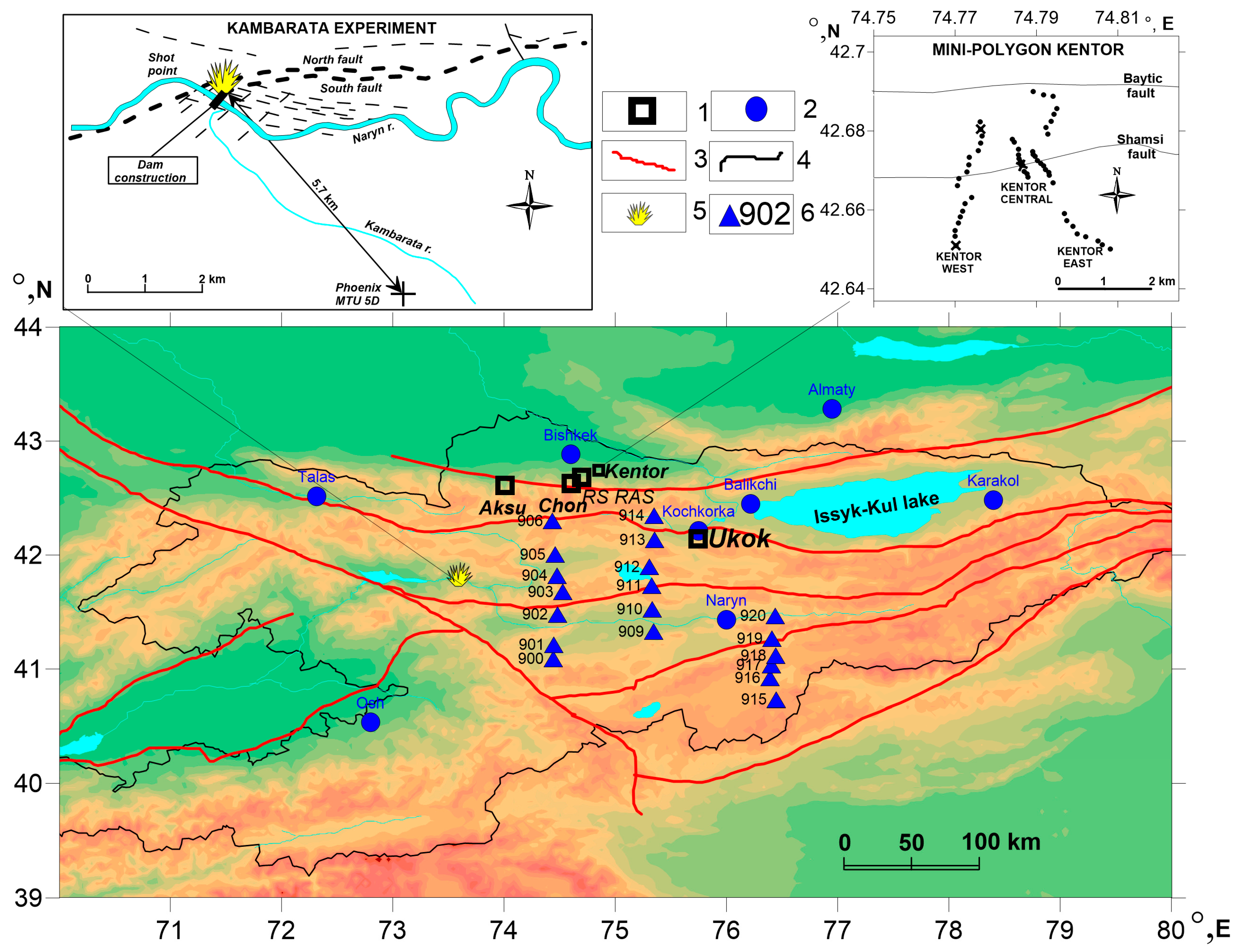
The methodology for processing MTS monitoring data is detailed in [31,49]. Figure 1 shows the network of monitoring points (deep MTS points) in the northern Tien Shan region.

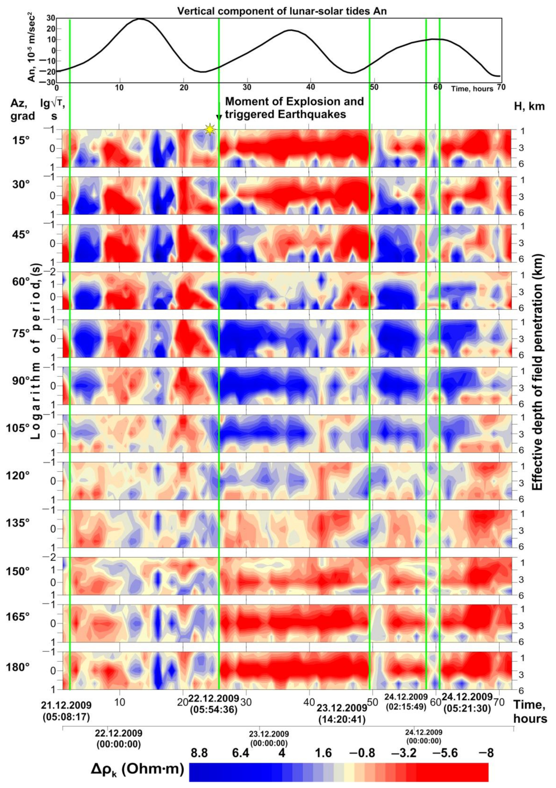
To represent the results of monitoring data processing, we utilized time–frequency series (TFS), which visualize the variability in measured electromagnetic field components with depth (logarithm of the sounding period) as the coordinate system is rotated by a certain angle (in degrees). Previously, some results showed good evidence of temporal variations. A widely researched study that is a very powerful example of a geodynamic man-made event with all known parameters (time, yield, volume) associated with initiated geodynamic natural events is the Kambarata blast-fill dam experiment. Figure 2 displays the TFS for the Kambarata point (top left panel in Figure 1) with a rotation step of α = 15° azimuth. The TFS shows the variations in apparent resistivity (Δρ_k), which represents the difference between the average and current values along the considered azimuth within a 72 h period [31,49]. This initial step allows for the analysis of anisotropy in physicoelectric parameters under different coordinate system orientations over continuous time. It is evident that the variations (Δρ_k) occur and exhibit uniqueness over time. These variations are influenced by changing telluric currents due to external factors such as lunar–solar tides, fluid dynamics, or man-made impacts on the lithosphere, as observed at the Kambarata point. The Kambarata 2 blast-fill dam is located in the geodynamically active and seismic part of the central Tien Shan [50]. The Kambarata explosion, which occurred on 22 December 2009 at 11:54 UTC in Kyrgyzstan (coordinates of the main explosion measured by GPS: 41.77467° N, 73.33122° E), was an exceptionally powerful event for geophysical monitoring. The explosion had a total yield of 2800 tons of TNT equivalent.

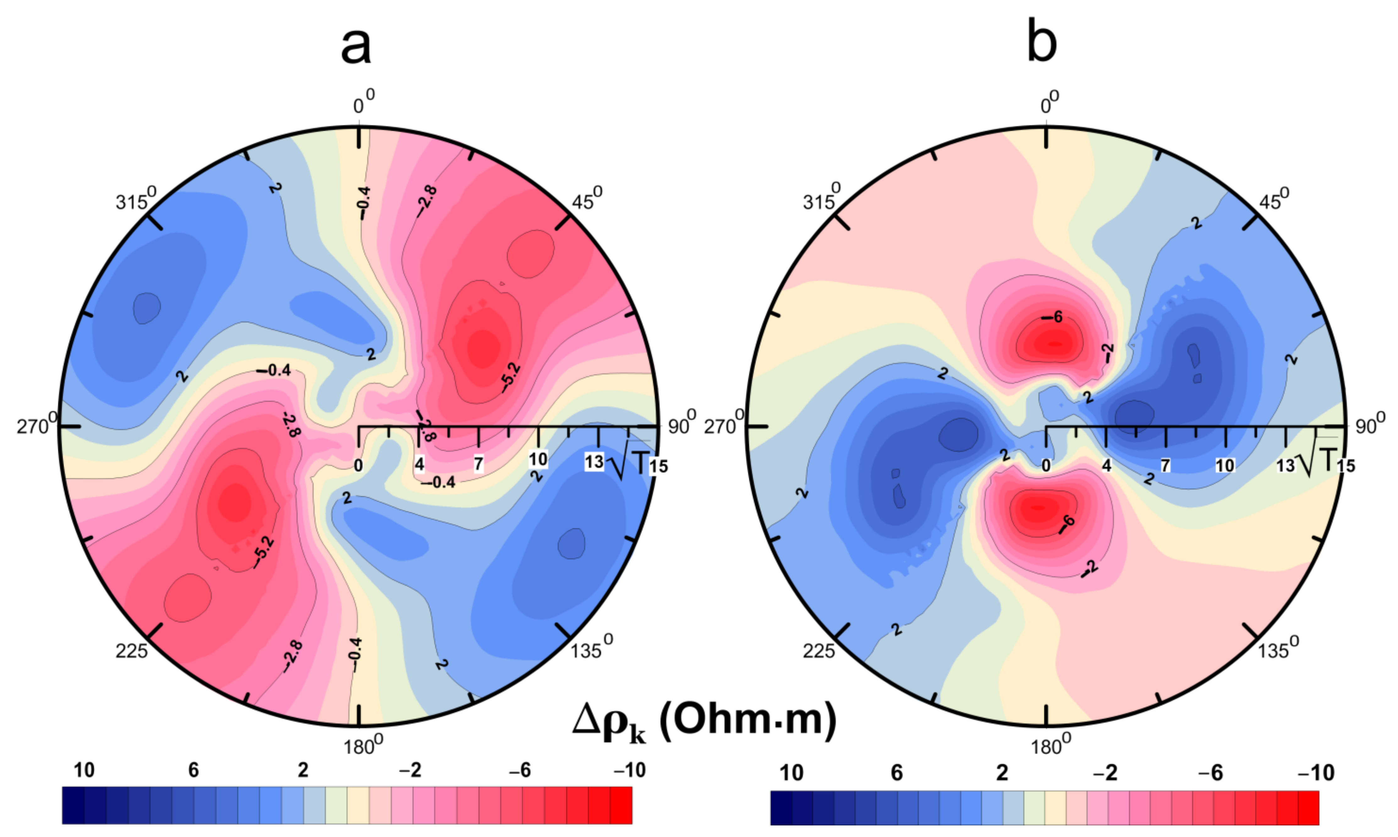
Additionally, another form of MTS monitoring data is represented in polar diagrams, which depict changes in electromagnetic parameters over a specific time period. Figure 3 demonstrates the behavior of apparent resistivity (ρ_k) before and after the Kambarata industrial explosion and subsequent earthquakes [31,49]. These polar diagrams serve as circular sounding monitoring tools that remain invariant regardless of the orientation of the instrument installation. This represents the second step in analyzing physicoelectric parameters with sounding period parameters.

Geodynamic processes manifest in the geological media as a result of stress and state imbalances. These processes involve both reversible and irreversible deformations [51,52,53] and occur slowly over extended periods, except for events like earthquakes. They also lead to structural and textural adjustments in rocks. Technogenic activities such as mining actively stimulate geodynamic processes as they disrupt the relative stress balance within geological media [51]. Shear stresses, tensile forces, and deformations occur, accompanied by continuous quasi-plastic flow, cracking, and the rupturing of rocks near mining sites [54].

In certain cases, fluid dynamics also contribute to geodynamic processes. For example, during oil extraction, the physical properties of the reservoir rock change as water fluid replaces the oil, leading to deformation (failure), fracturing of the rock matrix [55], and plastic deformation [56]. Another example concerns water tanks. Similarly, water-related factors such as changes in water level, leaching, and watering [54] can cause irreversible deformations and variations in the physical and mechanical properties of rocks.

2.2. Geodynamic Process Reflexion in the Physicoelectric Properties of Rocks

The variations in electrical resistivity are closely related to the process of rock deformation [57,58]. Deformation begins with the closure of fractures in the rock sample, and the extent of sample deformation nonlinearly depends on pressure. Simultaneously, the resistivity of the rock decreases due to the conductive surface increasing. As deformation progresses, elastic deformation exhibits a linear dependence on stress, leading to a linear decrease in resistivity. Increasing stresses initiate the development of both existing and newly formed cracks. Further stress buildup results in the release of accumulated elastic energy and a sharp increase in the number of cracks. At this point, an uncontrolled process of brittle fracture ensues, accompanied by a decrease in stresses and a sharp increase in resistivity. Thus, irreversible geodynamic processes manifest as the disruption of rock continuity and the formation of cracks, either without visible displacement or with displacement within their planes due to mechanical impacts caused by tectonic and non-tectonic forces [57,58].

Fracturing is a significant process occurring in all rocks under various geological conditions. The formed cracks are filled with fluids and particles from the deformable rock, altering the overall physical and mechanical properties of the rock [59]. In cases where highly conductive fluids fill the cracks, the structural features of the rock no longer play a role, and the electrical resistivity anisotropy coefficient decreases to unity as moisture content increases. However, in other cases, the anisotropy of electrical resistivity provides valuable information about the structural and textural features of the rock, such as layering, shearing, fracturing, etc. [39,60].

It is well established that resistivity anisotropy is highly sensitive to changes in rock stress. The anisotropy of electric conductivity correlates with the anisotropy of permeability in rock layers and serves as an indicator of the self-organized structure of the rock itself. Isotropy, therefore, represents a special case characterized by a disordered rock structure. To establish a quantitative relationship between the structural–textural and physicoelectric parameters of the rock, it is necessary to construct a phenomenological model of electrical resistivity that considers the structural features of the rock.

The geophysical literature has developed various types of structural phenomenological models and solutions for its numerical description. However, the calculation of electrical resistivity for such models is limited to transversely isotropic media, primarily due to the limited development of the Maxwell homogenization technique [13,61], which enables the transition from the local physicoelectric parameters of the media to macro-parameters.

2.3. Scope of Application for Effective Electromagnetic Parameters

Based on numerous field experiments (Figure 1), it has been observed that modern geodynamic processes lead to rock reorganization—changes in structural and textural characteristics. These modifications manifest as variations in the macro anisotropic electromagnetic parameters of the geological media at the macroscale level. These phenomena were first recognized by O.B. Barsukov [51]. To study these phenomena, it is necessary to explore the connection between the microstructure of rocks and their macroscopic parameters. This connection is addressed through the EMA theory, which considers effective electromagnetic parameters of micro-inhomogeneous media. The EMA theory assumes a relationship between the macroscopic parameters of the medium and its micro-composites, resulting in anisotropy [62]. Some electrical anisotropy studies started in the 20th century include those by Matlas and Habbejam [39], Berdichevsky et al. [63], and Lilley [64].

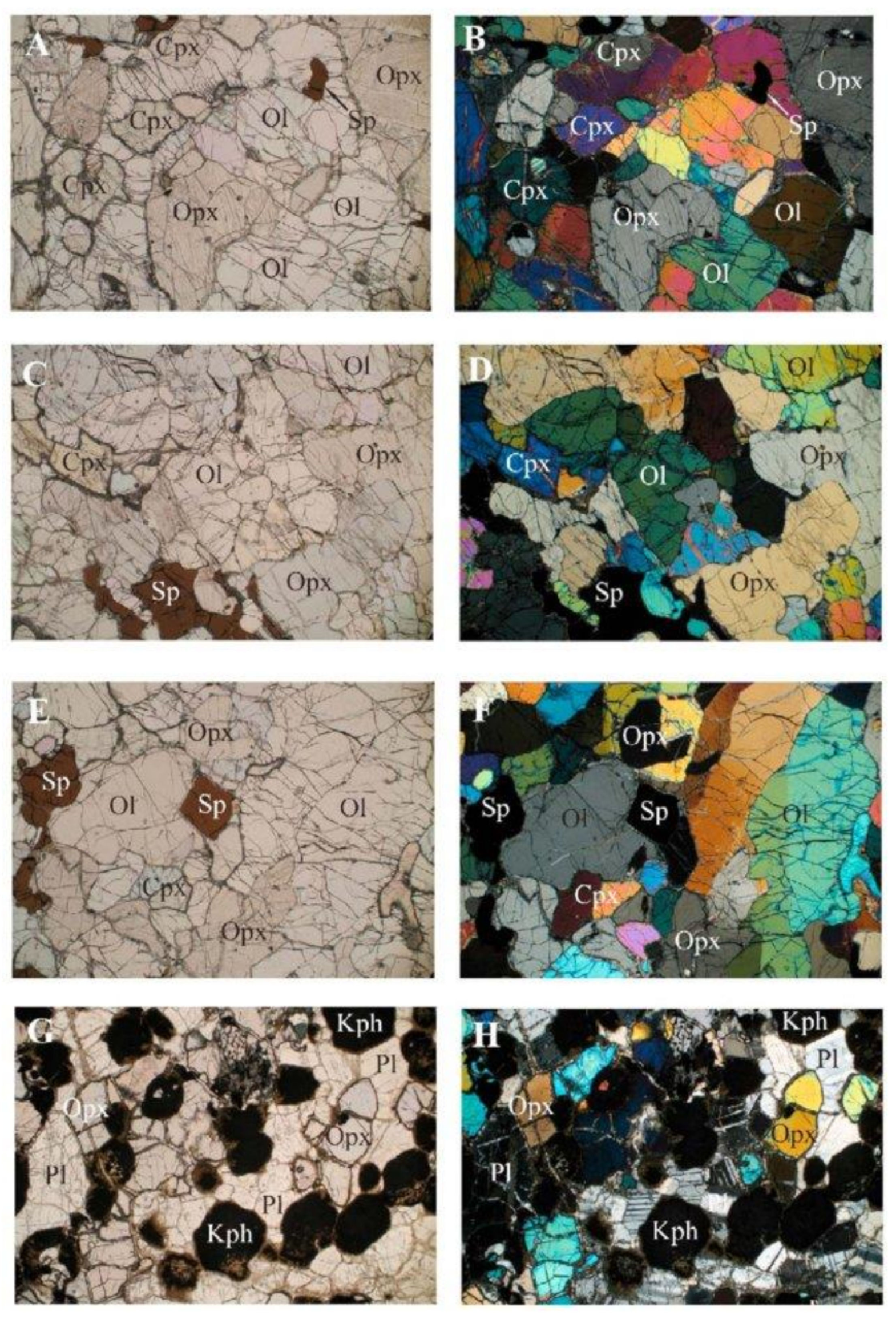
In the context of the central Tien Shan region and its deep-seated rocks (depicted in Figure 4), the investigation of effective electromagnetic parameters becomes crucial. These rocks exhibit a micro-heterogeneous nature, and understanding their behavior requires the calculation of effective electromagnetic parameters. This relationship aligns well with the observations made in the MTS turnaround analysis depicted in Figure 2 and Figure 3. By studying the relationship between the microstructure and macroscopic parameters of such rocks, we can gain insights into the anisotropic properties and their impact on electromagnetic monitoring data.

2.4. Calculations of the Effective Electric Conductivity of Rocks

Transition from the local electromagnetic characteristics of geological media to integral parameters is of great practical importance. Due to the large linear dimensions of the electromagnetic field sources and/or receivers, as well as the complex structure and vast volumes of the geological media, obtaining information about the local distribution of electromagnetic parameters within the rock is fundamentally impossible.

The problem of transitioning from local to integral parameters in electrical prospecting is analogous to the transition from microfields to macrofields in electrodynamics. Homogenization (averaging) of physically infinitesimal volumes transforms the Lorentz equations for microfields (describing the electromagnetic field under vacuum) into Maxwell’s equations, which describe the electromagnetic field in continuous media. The nature of charge location, movement, and interaction is not considered in Maxwell’s equations; instead, these phenomena are characterized through the relative dielectric and magnetic permeability and electric conductivity (ε, μ, σ) media parameters. Spatial and temporal averaging of microscale fields simplifies the solution of electromagnetic problems. However, solving Maxwell’s equations introduces the challenge of dealing with boundary conditions, which are absent in the Lorentz equations [66].

In geoelectrics during prospecting, a similar problem arises where each grain of rock-forming minerals has its own electromagnetic parameters, such as relative permittivity, magnetic permeability, and specific electrical resistivity. The complex relationship of electromagnetic parameters across spatial coordinates within rock samples poses significant challenges in solving Maxwell’s equations for such media. To overcome these difficulties, an additional stage of Maxwell homogenization is proposed. During this stage, Maxwell’s equations for a continuous media are averaged while considering the boundary conditions. Spatial averaging is performed over a small, physically finite volume, leading to the consideration of macroscale anisotropy in the effective resistivity and electric conductivity (σ^eff). We show this procedure in Appendix A.

There are different approximations of two-phase geological media that are still under investigation, and we introduce some of them here. The effective electric conductivity for spherical inclusions and layered media has been a subject of research since Maxwell’s work to obtain the effective resistivity of two-phase media [67,68]. Subsequently, many researchers have tackled this problem. An up-to-date view is supported by Kanaun [69,70]. According to S. Kanaun [69], we know that, “a homogeneous anisotropic conductive media with a set of anisotropic heterogeneities and its’ numerical solution, using Gaussian approximating functions around isolated anisotropic spherical and cylindrical inclusions in an anisotropic homogeneous host media was studied by numerous researchers” [71,72]. These approaches share a common model that describes the relationship between electric and elastic properties through effective properties by following Maxwell’s methodology [68]. Understanding the effective conductivity of bianisotropic media in terms of composites with anisotropic components is an up-to-date view proven by Kanaun [69]. V.R. Bursian developed a method [73] to obtain effective resistivity for layered media, demonstrating that the roundness of grains introduces anisotropic effects in electrical resistivity. A.S. Semenov [74] investigated the effective resistivity of paralloid-shaped inclusions, while A.M. Nechai [75] approximated real media with lumped parameters to obtain effective resistivity for cube-shaped inclusions. Similar conclusions were drawn in [6,7,8,9,10], which discuss the dependence of effective electrical conductivity on the number of inclusions. The authors also explored models that describe the dependence of elastic and electromagnetic parameters on grain shape, specifically the aspect ratio [76]. These parameters directly influence the distribution of thermal properties. In [13], the correlation between emerging effects in elastic parameters is explained as a consequence of the anisotropy of the geological environment. These approaches are based on the approximation of homogeneous anisotropic micro-heterogeneous media, providing a universal and common framework. V.P. Gubatenko [77] utilized averaging methods and expansion over the time period to consider the macroscale anisotropy tensor of electric conductivity (σ) in relation to the dielectric constant (ε). The effective resistivity of elliptical inclusions has been calculated from various perspectives by numerous researchers [69,78,79,80,81,82]. However, the full spectrum of anisotropy effects is not yet completely understood.

2.5. Theory: Electromagnetic Properties of Rock Capillarity

An important problem in the detailed description of the physicoelectric parameters of rocks is the complex configuration of hydrodynamic capillarity systems. In the context of the theory of effective media approximation (EMA), capillarity is treated as a conductor, while the host rock is considered an insulator. This allows for the geological parameter known as the tortuosity of the capillarity system to be obtained. EMA helps us to avoid special theory for electrokinetic (due to capillarity fluid mineralization) and mechano-electrical effects (rock failure and piezoelectric effects). The study of rocks with a developed capillarity system leads us to the formulation of new material equations known as bianisotropic media theory [83,84,85,86,87,88].

Bianisotropic media are characterized by linear electromagnetic properties described by general Maxwell’s equations:

$$J=\sigma E+\xi H,\begin{array}{cc}& \end{array}B=\zeta E+\mu H$$

(2)

rotH = σE + dD/dt, rotE = −dB/dt,

(3)

where J is the electric current density (A/m²), B is the magnetic induction intensity (Wb/m²), E is the electric field intensity vector (V/m), H is the magnetic field intensity vector (A/m), D = εE is the electric displacement vector (C/m²), ε is the dielectric constant, σ is the electric conductivity, and μ is magnetic permeability [68,89]. The items dD/dt and dB/dt are time derivatives. ξ and ζ are called effective parameters and are new in the theory and application of electrical prospecting and have not yet received definite designations. Equation (3) is given in differential form.

The effective parameters ξ and ζ are necessary for an adequate description of the electromagnetic behavior of a rock with a complex system of capillaries. They take into account the tortuosity of capillaries filled with a conducting fluid. The physical properties depend on the connectivity of joint patterns [60]. Physical interpretation of these parameters is associated with the generation of electric currents through induced electromotive force (parameter ξ) and the appearance of magnetic dipoles (parameter ζ) due to the presence of closed conductors in the media. These conductors, or closed loop currents, arise due to the complex geometry of the capillarity system, which can theoretically be divided into simpler elements. The electromagnetic behavior and electrical resistivity features of bianisotropic media have been previously studied [88,89,90,91,92]. In previous works by the authors, it was demonstrated that the effective parameters σ, μ, ξ, and ζ are 3 × 3 matrices because they correspond to three spatial components where anisotropy is observed [17,91]. In this study, we will focus on obtaining the effective parameters for a rock with a complex conductivity system.

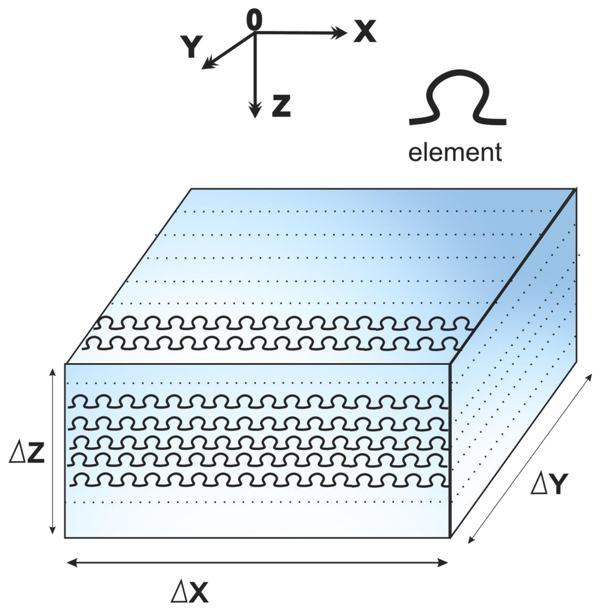
We first consider a rock volume that contains a system of capillaries with a complex configuration and infinite length (closed porosity). In this case, the electric conductivity of the media is solely determined by the conductivity of fluids filling the thin, extended capillaries. The idealized model of a horizontally layered system with capillaries is shown in Figure 5, where x, y, and z are spatial coordinates.

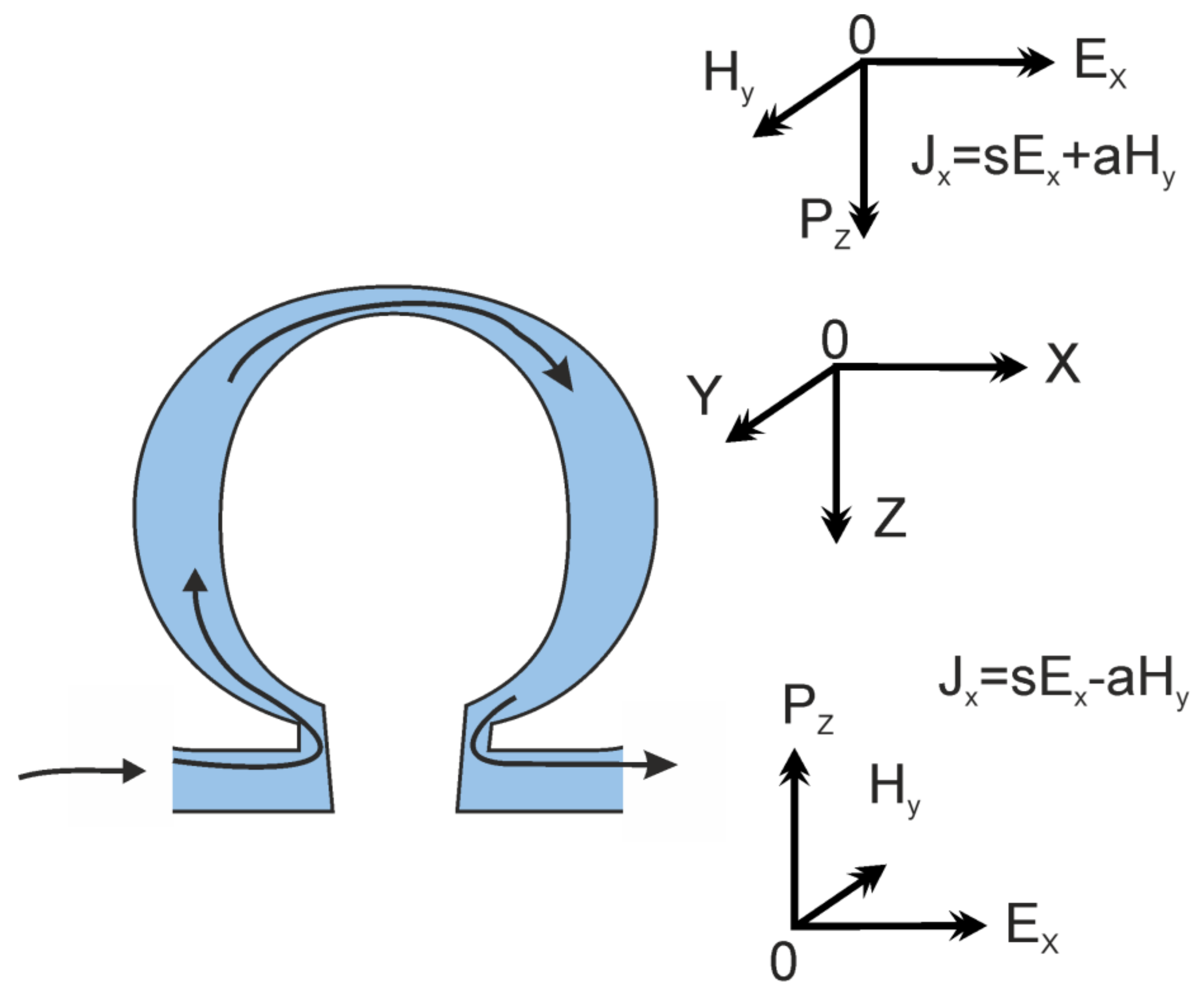
In this model, each individual capillary filled with fluid forms a rectilinear electric current that is galvanically connected to a loop-shaped capillary, referred to as the Ω (omega shape) inclusion [93,94]. The media in this case is considered dielectric, and the magnetic permeability remains constant along the entire length of the loop, equal to the magnetic permeability of a vacuum. This type of media is composite. More complex models can be found in [70].

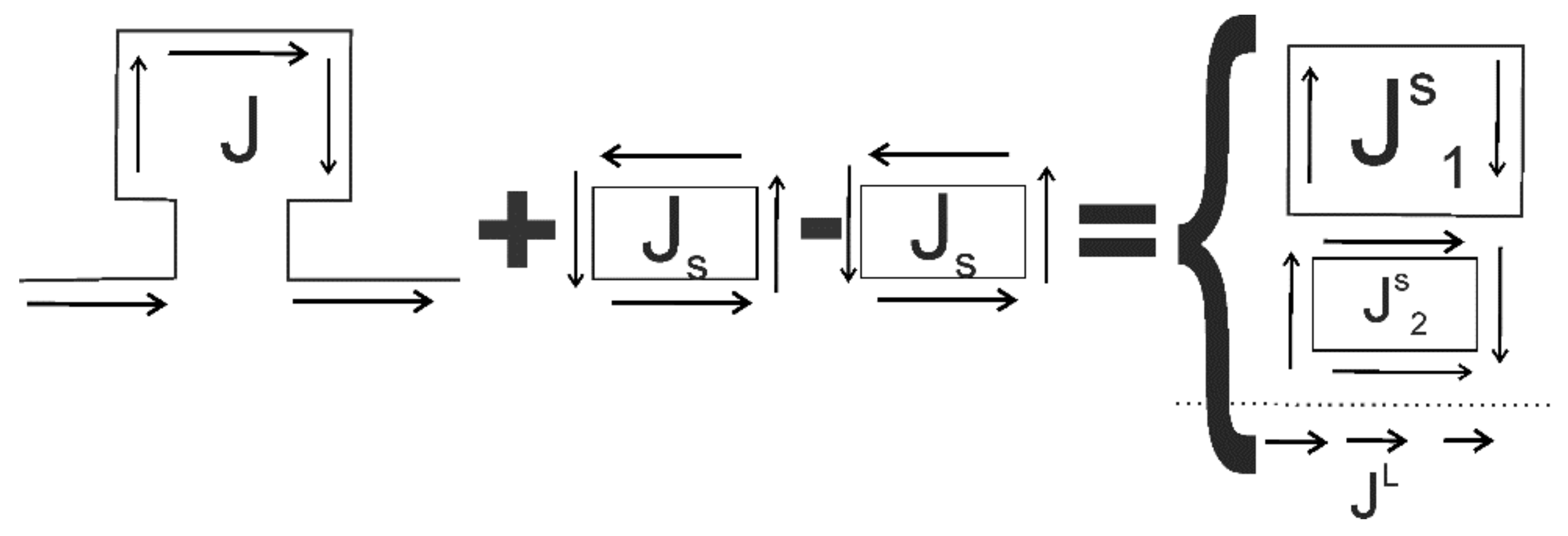
The problem of Maxwell homogenization is calculating the effective parameters for the suggested model of rock electric conductivity. To achieve this, we need to transform the complex system of electric current density J into a simpler configuration. The idea behind this transformation is shown in Figure 6 and can be represented as the addition and subtraction of electric current densities at the bottom of each segment of the Ω inclusion.

In Figure 6, it can be observed that by adding and subtracting currents, whose sum is zero, the complex system of currents within the Ω inclusion can be divided into current densities with simpler geometries: a straight current density, $J^s$, and two closed-loop current densities, $J_1^s$ and $J_2^s=-J^s$. The closed electric currents form two coaxial magnetic dipoles. We can now apply homogenization to calculate the effective electromagnetic parameters of the capillarity system. Closed currents, similar to magnetic dipoles, are volume parameters, and the homogenization process reduces them to calculate the average magnetic moment for a given volume. Homogenization of a system of coaxial straight currents does not present significant difficulties. It is important to note that a similar transformation can be applied to more complex capillary flow geometries.

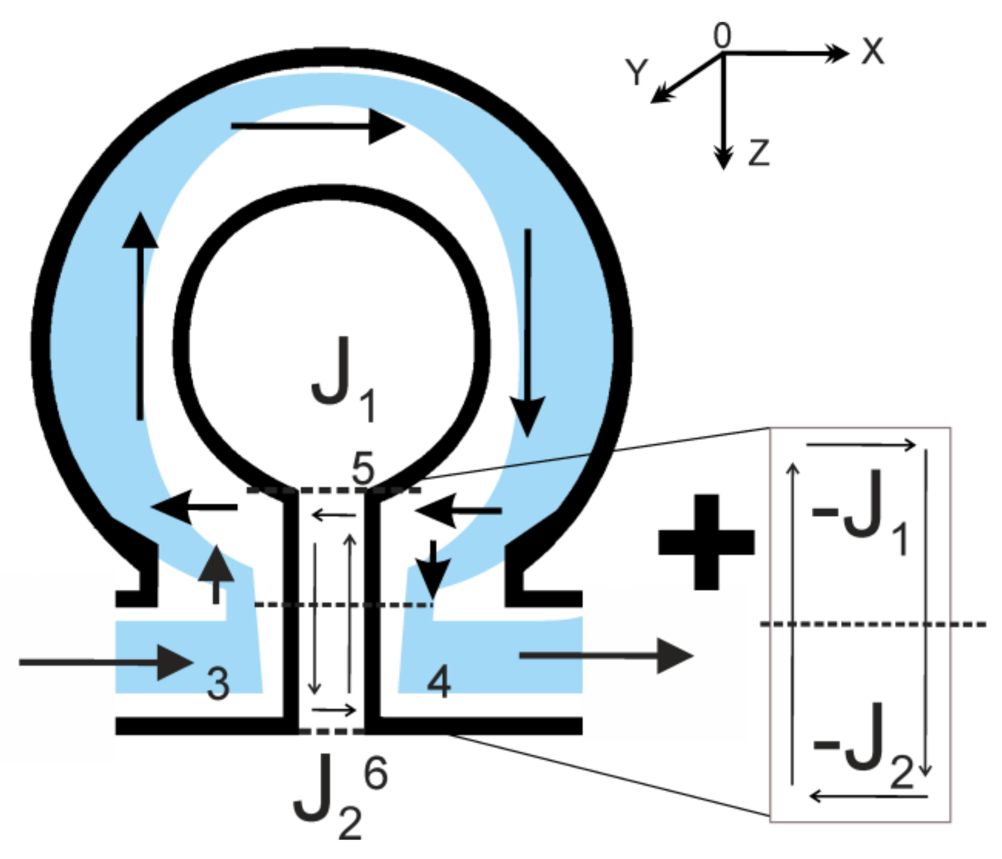
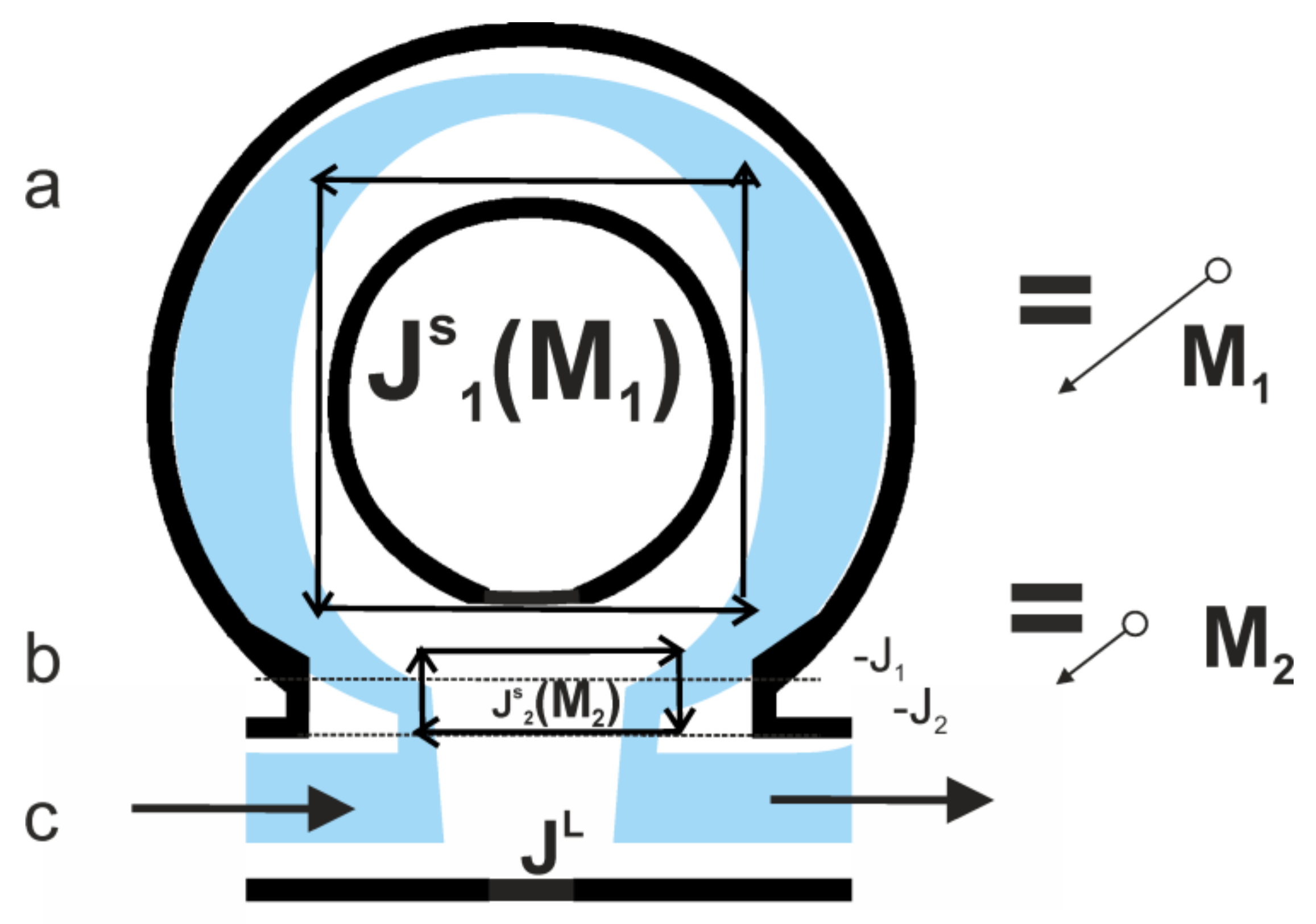
The scheme for separating electric current densities, taking into account capillary size, is illustrated in Figure 7 and Figure 8, along with the distribution of currents in the capillaries [94,95].

The loop current density in the inset (Figure 8b) is divided by a dotted line into two components, $J^s=J_1+J_2$. The need for such a division will be clear from the following discussion. According to the procedure described above, the system of currents is added and subtracted from the current at the bottom of the Ω inclusion (Figure 7), provided that

$$\begin{array}{l}{\displaystyle \underset{3}{\overset{4}{\int }}{(J+J_1+J_2)}_{z}dxdy}=0,\\ {\displaystyle \underset{5}{\overset{6}{\int }}{(J_1+J_2)}_{x}dxdy}=0,\end{array}$$

where points 3, 4, 5, and 6 mark the cross sections of the capillaries where the total current density must be zero. The first condition eliminates currents that are normal to the surface of the capillarity, as shown by the dashed line in Figure 8a,b. The second condition relates the current density in the closed part of the capillarity to the current in its rectilinear part (Figure 8c). In other words, the introduced currents do not change Maxwell’s equations, but the currents in the Ω inclusion are presented as a sum of three components (Figure 8): a rectilinear current density ($J^1$) and two closed current densities. The latter have the same direction and are written in the form $J_1^s=rot{M}_1$ and $J_2^s=rot{M}_2$ (Figure 8), where closed currents are the curls, which describe the rotation of a vector field enclosing charge M₁ in a bigger loop and M₂ in a smaller loop. In this case, the electric currents in the newly formed currents are continuous. Since the currents are relatively small, they will be ignored.

The original Maxwell’s equations from Equation (3), where σ is the electric conductivity of the capillarity and μ is the magnetic permeability of the media, can then be transformed into the complex form with the imaginary unit i:

$$\begin{array}{l}rotH=\sigma E+i\omega D=J+J_1-J_1+J_2-J_2=J^1+J_1^s+J_2^s,\\ =rot{J}^1+rot{M}_1+rot{M}_2\\ rotE=-i\omega \mu H.\end{array}$$

(4)

The model is now supplemented with a capillarity system oriented along the Y axis and not interacting with the original system (Figure 8) and a system of linear capillaries oriented along the vertical Z axis under conductivity, at which the conductivity of the rock will be the same in all directions. Ignoring the interaction between Ω inclusions, we could apply coordinate averaging for electrical conductivity: ${\sigma }^e=\frac{1}{\frac{1}{\Delta X}{\displaystyle \underset{L}{\int }\frac{1}{\frac{1}{S_x}{\displaystyle \underset{S_x}{\int }\sigma dydz}}}dx}$ (see Appendix A). Therefore, the material equations (Equation (2)) averaged over the rock volume in complex form are written as

$$\begin{array}{l}J=i{J}_x=i{\sigma }^e{E}_x-ii\omega \mu {\alpha }^e{H}_y,\\ B=j\mu {\beta }^e{E}_x+\mu H,\end{array}$$

(5)

where ${\alpha }^e=n\alpha$; ${\beta }^e=n\beta {\sigma }^{*}$ are some parameters of pore and capillarity tortuosity; n is a quantity of inserts in a volume unit; i and j are capillarity units inside the volume; and x, y, and z are spatial coordinates. Thus, the effective parameters ξ and ζ from Equation (2) become complex $\xi =i\omega \mu {\alpha }^e$ and $\xi =\mu {\beta }^e$.

Accordingly, other spatial components are

$$\begin{gathered} J_x=\sigma E_x-i\omega \mu \alpha H_y; B_x=\mu H_x-\mu \beta E_y; \\ {J}_y=\sigma E_y+i\omega \mu \alpha H_x; B_y=\mu H_y+\mu \beta E_x; \end{gathered}$$

$J_z=\sigma E_z$; $B_z=\mu H_z$, because the model is horizontally layered.

The material equations in general view then take the complex vector form

$$\begin{array}{l}J=\stackrel{⌢}{\sigma }E-i\omega \mu \stackrel{⌢}{\alpha }H,\\ B=\mu \stackrel{⌢}{\beta }E+\stackrel{⌢}{\mu }H,\end{array}$$

(6)

where $\stackrel{⌢}{\sigma }=\left(\begin{array}{ccc}\sigma & 0& 0\\ 0& \sigma & 0\\ 0& 0& \sigma \end{array}\right)$; $\stackrel{⌢}{\alpha }=\left(\begin{array}{ccc}0& \alpha & 0\\ -\alpha & 0& 0\\ 0& 0& 0\end{array}\right)$; $\stackrel{⌢}{\beta }=\left(\begin{array}{ccc}0& -\beta & 0\\ \beta & 0& 0\\ 0& 0& 0\end{array}\right)$; $\stackrel{⌢}{\mu }=\left(\begin{array}{ccc}\mu & 0& 0\\ 0& \mu & 0\\ 0& 0& \mu \end{array}\right)$.

The bianisotropic effective parameters $\stackrel{⌢}{\alpha }$ and $\stackrel{⌢}{\beta }$ are antisymmetric matrices, and their structure depends on the orientation of the Ω inclusion relative to the straight, linear part of the capillarity. For instance, $\stackrel{⌢}{\alpha }$ and $\stackrel{⌢}{\beta }$ change signs (opposite signs) when the Ω inclusion is rotated by 180° relative to the rectilinear segment (resulting in an L-shaped media). Other orientations lead to different structures for matrices $\stackrel{⌢}{\alpha }$ and $\stackrel{⌢}{\beta }$. For example, a 90° rotation gives rise to diagonal matrices known as Tellegen media [96].

In a constant electromagnetic field, the effects of bianisotropic media disappear in an electric field but remain present in a magnetic field. One remarkable property of bianisotropic media is the violation of the principle of reciprocity, which can be illustrated in a simple manner (Figure 9).

As a result, the electric current density becomes the sum of the conduction current (from the linear part of the capillarity) and the induction of the magnetic field due to the loop. When the electromagnetic field propagates from top to bottom (from the first source), the electric current in the Ω inclusion is the sum of the electric current from the linear part of the capillarity and the electric current density induced by the magnetic field’s induction in the loop ($J_x=\sigma E_x+a{H}_y$) (Figure 9). Conversely, when the electromagnetic field propagates from bottom to top (from the second source), the electric current in the Ω inclusion is the sum of the electric current density from the linear part of the capillarity and another, which is induced by the magnetic field’s induction in the loop but with a negative sign ($J_x=\sigma E_x-a{H}_y$). Therefore, the electric current density either increases or decreases depending on the direction of electromagnetic field propagation. This effect can be explained formally as follows:

If we consider the system of Maxwell’s equations (Equation (5)) in a homogeneous media with electromagnetic parameters, σ₀ is media conductivity, μ₀ is the media permeability, and iωD is equal to 0:

$$rotH={\sigma }_{0}E,$$

$$rotE=-i\omega {\mu }_{0}H.$$

(7)

If we represent magnetic field $\tilde{H}=fH$ and electric field $\tilde{E}=qE$ as multiplexing by functions f and q, which will be defined below, then Maxwell’s equations for these vectors of the electromagnetic field, taking into account (7), take the form

$$\begin{array}{l}rot\tilde{H}=rotfH=frotH+gradf\times H={\sigma }_{0}f\frac{q}{q}E+\frac{gradf}{f}\times fH={\sigma }_0\frac{f}{q}\tilde{E}+\frac{gradf}{f}\times \tilde{H}\\ rot\tilde{E}=rotqE=qrotE+gradq\times E=-i\omega {\mu }_{0}q\frac{f}{f}H+\frac{gradq}{q}\times qE=-i\omega {\mu }_0\frac{q}{f}\tilde{H}+\frac{gradq}{q}\times \tilde{E}\end{array}$$

Considering $f=e^d$ and $q=e^c$ are exponential functions, where $d$ and $c$ are some functions of spatial coordinates, we obtain [94]

$$\begin{array}{l}rot\tilde{H}={\sigma }_0{e}^{d-c}\tilde{E}+gradd\times \tilde{H},\\ rot\tilde{E}=-i\omega {\mu }_0{e}^{c-d}\tilde{H}+gradc\times \tilde{E}.\end{array}$$

Particularly, assuming $d=c={\alpha }_{23}x+{\alpha }_{13}y+{\alpha }_{12}z=g$, we obtain

$$gradg\times =\left(\begin{array}{ccc}0& -{\alpha }_{12}& {\alpha }_{13}\\ {\alpha }_{12}& 0& -{\alpha }_{23}\\ -{\alpha }_{13}& {\alpha }_{23}& 0\end{array}\right)=\alpha =\beta ,$$

(8)

from which we obtain the system of Maxwell’s equations for bianisotropic media:

$$\begin{array}{l}rot\tilde{H}={\sigma }_0\tilde{E}+\alpha \tilde{H},\\ rot\tilde{E}=-i\omega {\mu }_0\tilde{H}+\beta \tilde{E}.\end{array}$$

(9)

Thus, violation of the principle of reciprocity (ERT) in bianisotropic media leads to exponential growth of the electromagnetic field in one direction and an exponential decrease in the opposite direction (Equation (9) vs. Equation (6)). This property can be utilized to study the tortuosity of the capillarity system of electric conductivity in rocks.

However, due to the challenges in solving forward and inverse problems for bianisotropic media, there is currently no scientifically justified technical solution for their use in electromagnetic monitoring. Some progress has been made in modeling inversion and interpretation of magnetotelluric responses, as shown in [97]. Additionally, there are solutions for forward problems [98,99]. Section 3.2 presents geological object models for bianisotropic media using EMA theory. It is worth noting that the development of bianisotropic media EMA began in the 1920s, and contributions by V.R. Bursian [73] in the Russian-speaking sector have been fundamental to the development of the fundamental foundations of electrodynamics.

3. Results and Discussion

3.1. The Monitoring of Geodynamic Processes

The current tectonic regime of submeriodional transpression in the Tien Shan region leads to changes in the integral macroscopic parameters of geological media, resulting in variations and anomalies being observed in continuous measurements of electrophysical parameters such as apparent electrical resistivity. Successful monitoring examples, such as the Kambarata experiment, demonstrate that certain azimuthal rotations make the apparent electrical resistivity most sensitive to simultaneous seismic events. The developed effective media approximation theory allows for mathematical definition of the effective electrical conductivity tensor (σ^eff) for gradient anisotropic media by averaging the spatial dependence of parameters over a small, physically finite volume.

Experimental data for the Tien Shan region demonstrate clear decreases and increases in electrical resistivity values along orthogonal azimuths (Figure 2 and Figure 3). Cleavage microcracks, which can be parallel or perpendicular, are common in rock masses and contribute to the observed anisotropy in changing physical parameters. The present study identifies key points with complex relationships between variations in apparent electrical resistivity and the stress–strain state of crustal parts in order to investigate geodynamic processes in seismically active zones. Slow fluid redistribution between fracture and pore systems during seismic event preparation is also reflected in variations in electric conductivity, as shown in [29].

Effective parameters such as electric conductivity are useful for studying the impact on geological media, and EMA theory allows for their manipulation. Apparent resistivity and impedance phase values are employed to assess effective parameters, which are highly sensitive to geological media. The choice of coordinate system affects the effective electric conductivity, and switching to another system can result in gradient anisotropic media.

Appendix A provides general expressions for effective electric conductivity, while the following subsection explores several models of rock deformation and their reflection in macro anisotropic electrical parameters that are relevant for active electromagnetic monitoring considering different kinds of monitoring system configurations.

3.2. The Geodynamic Model Examples

Homogenization, which represents the physical meaning of mean value averaging operations, is valid for these selected media models. There are three models of bianisotropic media: fracturing in the rock mass, quasi-plastic deformation of rocks, and rock failure near the borehole. Partly, examples and descriptions of the propagation of an electromagnetic field in anisotropic and bianisotropic two-dimensional horizontally inhomogeneous layered media and radially inhomogeneous media were considered by the authors of [81]. Solutions for the forward problems of geoelectrics are mainly limited to special study cases of bianisotropic media. For example, for a model of two-phase composite materials with an anisotropic microstructure (non-randomly oriented non-spherical inclusions), a clear correlation was established between two groups of anisotropic effective properties: conductivity and elasticity. Here, we show three models: fracturing in the rock mass, quasi-plastic deformation of rocks, and rock failure near the borehole. For the below model calculation, please refer to the PhD thesis of P.N. Aleksandrov [17].

3.2.1. Model of Fracturing in the Rock Mass

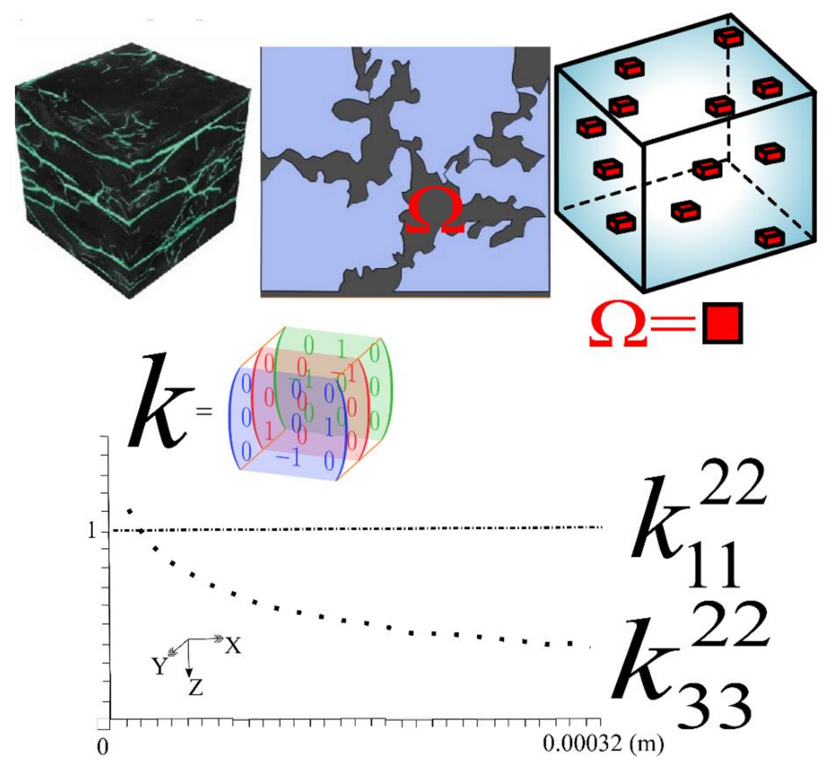
As the analysis of the manifestation of geodynamic processes shows, they are expressed in the structural and textural rearrangement of the rock. We will consider these transformations using the example of fracture formation in fractured carbonate reservoirs. At first, vertical cracks appear in the initially layered rock model under the influence of irreversible deformations. Such a model, corresponding to the model shown in Appendix A (Equation (A2)), can be described by the following distribution of local electrical parameters:

$$\sigma =10X(x)Y(y)Z(z),$$

where

$$X(x)=\left\{\begin{array}{c}0.01,x=[0,0.2]\\ 10,x=[0.02,0.02+h]\\ 0.01,x=[0.02+h,0.04+h]\end{array}\right.; Y(y)=\left\{\begin{array}{c}1,y=[0,0.02]\\ 0.15,y=[0.02,0.04]\\ 0.5,y=[0.04,0.06]\\ 2,y=[0.06,0.061]\\ 0.3,y=[0.061,0.081]\end{array}\right.; Z(z)=\left\{\begin{array}{c}1,z=[0,0.2]\\ 0.1,z=[0.2,2.2]\end{array}\right..$$

The dependence of the effective tensor of resistivity on macroscale anisotropy is shown in Figure 10.

The behavior of the graph of the anisotropy coefficient shows that the macro anisotropic characteristics of the rock in terms of electric conductivity depend, and quite strongly, on the presence, thickness, and electric conductivity of cracks. In this case, the macroscale anisotropy coefficients change to

$$k_{22}^{11}=\sqrt{\frac{{\rho }_{22}}{{\rho }_{11}}}=[1.26,0.38]; k_{33}^{11}=\sqrt{\frac{{\rho }_{33}}{{\rho }_{11}}}=[1.29,0.38]; k_{33}^{22}=\sqrt{\frac{{\rho }_{33}}{{\rho }_{22}}}=[1.01,1.01]$$

when the crack opening degree (h) changes from 0 to 3.2·10⁻⁴ m.

This change is sufficient and permits us to assert that the resistivity macroscale anisotropy tensor is an informative parameter sensitive to modern geodynamic processes. Additionally, we conclude that it is necessary to monitor all elements of the macroscale anisotropy tensor because, as follows from the above calculations, the anisotropy coefficient $k_{33}^{22}$ varies slightly depending on the crack opening degree. Thus, all the elements of the macroscale anisotropy tensor are specific objects of research in active electromagnetic monitoring. The following model confirms this fact.

3.2.2. Model of the Quasi-Plastic Deformation of Rocks

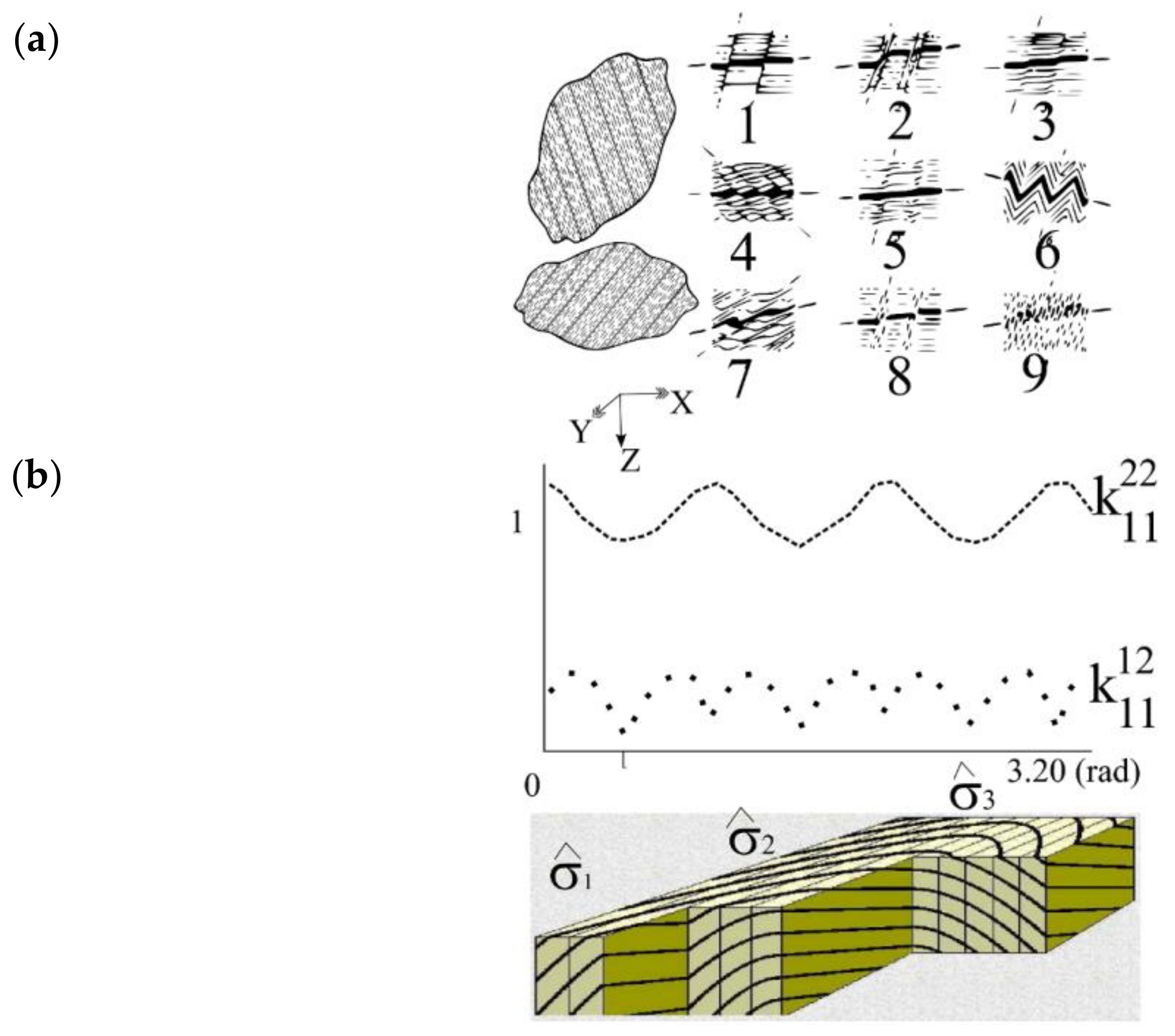
The model shown in Figure 11 characterizes irreversible geodynamic processes in the layer pack as a result of quasi-plastic movement of the rock mass. It assumes that the geoelectric boundaries do not change in the layer unit. The layers themselves undergo changes in terms of the formation of micro-dislocations in the form of cleavage (see [100,101]) in each layer.

In a Cartesian coordinate system, a two-dimensional model is analogous to strata interlayering. Each layer, with a thickness of h_i, is characterized by the anisotropy tensor of electric conductivity,

$${\sigma }_i=\left(\begin{array}{cc}{\sigma }_{11}^i& 0\\ 0& {\sigma }_{22}^i\end{array}\right),$$

with constant elements of this tensor. The macroscale anisotropy tensor of effective electric conductivity will then have the form

$${\sigma }^{eff}=\left(\begin{array}{cc}{\sigma }_{11}& 0\\ 0& {\sigma }_{22}\end{array}\right),$$

where for n layers

$${\sigma }_{11}=\frac{1}{{\displaystyle \sum _{i=1}^n{h}_i}}{\displaystyle \sum _{i=1}^n{\sigma }_{11}^i{h}_i}; {\sigma }_{22}=\frac{1}{\frac{1}{{\displaystyle \sum _{i=1}^n{h}_i}}{\displaystyle \sum _{i=1}^n\frac{h_i}{{\sigma }_{22}^i}}}.$$

The anisotropy coefficient is equal to

$$k_{22}^{11}=\sqrt{\frac{{\sigma }_{11}}{{\sigma }_{22}}}=\sqrt{\frac{1}{{\displaystyle \sum _{i=1}^n{h}_i}}{\displaystyle \sum _{i=1}^n{\sigma }_{11}^i{h}_i}\frac{1}{{\displaystyle \sum _{i=1}^n{h}_i}}{\displaystyle \sum _{i=1}^n\frac{h_i}{{\sigma }_{22}^i}}}.$$

Let us consider one important case observed experimentally that does not yet have a theoretical explanation. In some cases, during field and laboratory studies of geological objects, it is noted that the anisotropy coefficient is

$$k_{22}^{11}=\sqrt{\frac{{\rho }_{22}}{{\rho }_{11}}}=\sqrt{\frac{{\sigma }_{11}}{{\sigma }_{22}}},$$

where ρ₁₁ is the resistivity of the layered media along the strata and ρ₂₂ is the resistivity of the layered media across the strata, which may be less than 1.

To explain this fact, let us consider a two-dimensional model of a three-layer media, each layer of which has the following mesoanisotropy of electric conductivity: the first layer with electric conductivity and thickness, and the second with a thickness and electric conductivity tensor:

$${\sigma }_2=\left(\begin{array}{cc}{\sigma }_{11}& 0\\ 0& {\sigma }_{22}\end{array}\right),$$

where the third layer is isotropic with electric conductivity σ₃ and thickness h₃.

The macroscale anisotropy tensor of the effective electric conductivity then takes the form

$${\sigma }^{eff}=\left(\begin{array}{cc}\frac{{\sigma }_1{h}_1+{\sigma }_{11}{h}_2+{\sigma }_3{h}_3}{h_1+h_2+h_3}& 0\\ 0& \frac{h_1+h_2+h_3}{h_1{\rho }_1+h_2{\rho }_{22}+h_3{\rho }_3}\end{array}\right)$$

where ${\rho }_1=\frac{1}{{\sigma }_1}$, ${\rho }_{22}=\frac{1}{{\sigma }_{22}}$, and ${\rho }_3=\frac{1}{{\sigma }_3}$.

For h₁ = h₂ = h₃ and σ₁ = σ₃ = 1/ρ = σ, the anisotropy coefficient $k_{22}^{11}$ takes the form

$$k_{22}^{11}=\sqrt{\frac{5+2(\sigma {\rho }_{22}+{\sigma }_{11}\rho )}{9}}.$$

Hence, it follows that the macroscale anisotropy coefficient $k_{22}^{11}$ is greater than 1 at $\sigma {\rho }_{22}+{\sigma }_{11}\rho >2$ and less than 1 at $\sigma {\rho }_{22}+{\sigma }_{11}\rho <2$.

Thus, the presence of an anisotropic layer in a stack of layers can lead to an anisotropy coefficient of less than 1.

Let us next consider the case of interlayering of anisotropic strata. Each layer of this model is characterized by the electrical conductivities ${\sigma }_{11}^i$, ${\sigma }_{22}^i$ (in the case of electric conductivity tensor reduction to a diagonal form), and ${\alpha }_i$ by the rotation angle of the anisotropy tensor relative to the selected coordinate system:

$${\sigma }_i=\left(\begin{array}{cc}{\sigma }_{11}^i{\cos }^2{\alpha }_i+{\sigma }_{22}^i{\sin }^2{\alpha }_i& ({\sigma }_{22}^i-{\sigma }_{11}^i)\cos {\alpha }_i\sin {\alpha }_i\\ ({\sigma }_{22}^i-{\sigma }_{11}^i)\cos {\alpha }_i\sin {\alpha }_i& {\sigma }_{11}^i{\sin }^2{\alpha }_i+{\sigma }_{22}^i{\cos }^2{\alpha }_i\end{array}\right).$$

Each layer has a thickness of $h_i$. The described model is consistent with model (Appendix A, Equation (A9)).

We will next consider the dependence of the effective tensor of resistivity’s macroscale anisotropy on changes in the anisotropic characteristics of the intermediate layer. For this purpose, calculations were carried out for a three-layer model with the following parameters:

$$\begin{array}{l}{\sigma }_1=0.1, h_1=0.01,\\ {\sigma }_{11}^2=0.1, {\sigma }_{22}^2=0.2, {\alpha }_2=\left[0.2\pi \right], h_2=0.01,\\ {\sigma }_{11}^3=0.1,h_3=0.01.\end{array}$$

In this model, the angle of rotation of the anisotropy tensor of the second layer was changed from 0 to $2\pi$. Graphs of changes in the coefficients of macroscale anisotropy, $k_{11}^{12}=\sqrt{\frac{{\rho }_{12}}{{\rho }_{11}}}$ and $k_{11}^{22}=\sqrt{\frac{{\rho }_{22}}{{\rho }_{11}}}$ depending on the angle, are shown in Figure 11. From the behavior of these graphs, we observe that the diagonal elements of the macroscale anisotropy tensor change slightly depending on the angle rotation, while the off-diagonal elements change very significantly. The absolute value of the off-diagonal elements is changed to the measurable value.

A similar approach to calculating the effective parameters is valid in any other orthogonal coordinate system where the coordinate planes coincide with the planes of discontinuity in the electromagnetic parameters. In other words, when the representation in a certain coordinate system is valid, the description of the microstructure takes the form of a product of isolated functions of coordinates in a given coordinate system. As an example, consider a cylindrical coordinate system, which is important for studying the dynamics of physicoelectric parameters associated with the destruction of rocks near production boreholes.

Thus, in the examples considered for a Cartesian coordinate system and for a cylindrical one the macro anisotropic electrical parameters became gradient anisotropic media when passing from one coordinate system to another.

Obtaining such information is associated with some methodological difficulties. The known technique of azimuthal resistivity sounding (ARS) is aimed at measuring the apparent anisotropy in direct current methods. However, there are no grounds to unambiguously recognize this setup as the only possible option for measuring the anisotropy of the electric conductivity of the media, since other installations also carry information about the anisotropy of the media.

3.2.3. Model of Rock Failure near the Borehole

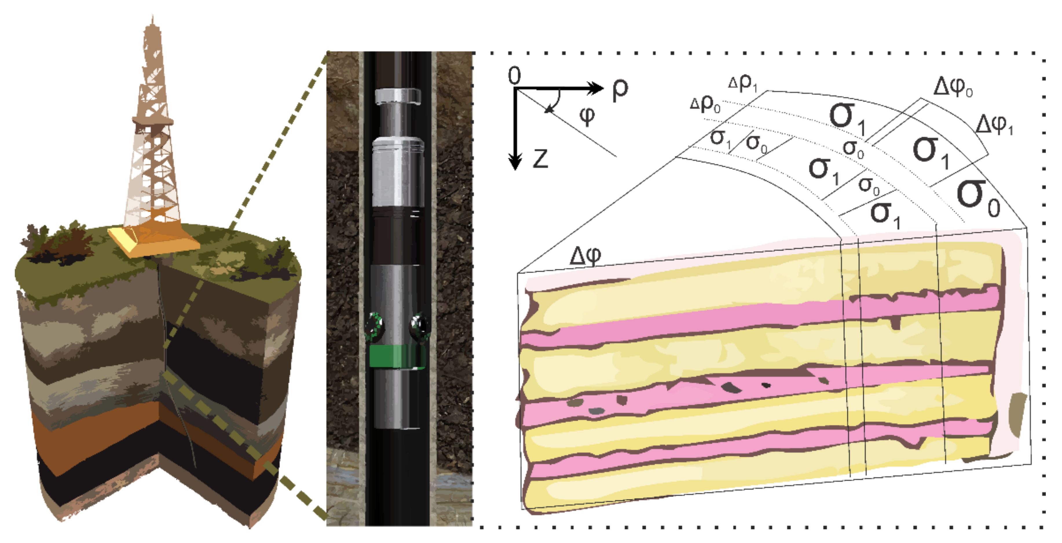
The borehole model (Figure 12) reflects irreversible geodynamic processes near wells. It mainly characterizes tensile deformations, due to which radial and azimuthal fracture cracks are formed. The development of fracturing and the accompanying process of filling the fractures with fluid will be accompanied by a change in the resistivity of the near-well space. As a result, the macroscopic geoelectric characteristics of the rock near the well become azimuthally anisotropic.

To determine the effective electric conductivity of the rock near the well, we use the cylindrical coordinate system with new coordinates, namely $\rho$, $\varphi$, and $z$, where $\rho$ is the radial coordinate, $\varphi$ the azimuthal coordinate, and $z$ the vertical coordinate. As the homogenization volume, we select a segment bounded by an $\Delta \varphi$ angle, $\Delta \rho$ radius, and $\Delta z$ thickness.

We consider the model of the media to be uniform along the Z axis. The inclusions have sizes of $\Delta {\rho }_1$, $\Delta {\varphi }_1$, and $\Delta z_1$ and electric conductivity of ${\sigma }_1$, while the size of the pore space is $\Delta {\rho }_0$ with electric conductivity of ${\sigma }_0$(Figure 12).

In the general case, the electric conductivity in the entire homogenization volume cannot be represented as a product of isolated functions of coordinates. However, in each separate layer, bounded in Figure 12 by the dotted line, electric conductivity has the following appearance. Therefore, we first average the electric conductivity in each layer over the spatial coordinates.

At $\rho \in \Delta {\rho }_1$,

$${\sigma }^{eff}=\left(\begin{array}{ccc}{\sigma }_1\frac{\Delta {\phi }_1}{\Delta \phi }+{\sigma }_0\frac{\Delta {\phi }_0}{\Delta \phi }& 0& 0\\ 0& \frac{1}{\frac{1}{{\sigma }_1}\frac{\Delta {\phi }_1}{\Delta \phi }+\frac{1}{{\sigma }_0}\frac{\Delta {\phi }_0}{\Delta \phi }}& 0\\ 0& 0& {\sigma }_1\frac{\Delta {\phi }_1}{\Delta \phi }+{\sigma }_0\frac{\Delta {\phi }_0}{\Delta \phi }\end{array}\right),$$

where $\Delta \varphi =\Delta {\varphi }_1+\Delta {\varphi }_0$; if $\rho \in \Delta {\rho }_0$, ${\sigma }^{eff}={\sigma }_0$.

With this operation, the transition to the (radially) layered anisotropic model (1.6) is carried out. Passing this to the entire homogenization volume, i.e., averaging (radially) layered anisotropic media, we finally obtain

$${\sigma }^{eff}=\left(\begin{array}{ccc}{\sigma }_{11}& 0& 0\\ 0& {\sigma }_{22}& 0\\ 0& 0& {\sigma }_{33}\end{array}\right),$$

(10)

where $\Delta \rho =\Delta {\rho }_1+\Delta {\rho }_0$;

$$\begin{array}{l}{\sigma }_{11}=\frac{1}{\frac{\Delta {\rho }_1}{\Delta \rho }\frac{1}{{\sigma }_1\frac{\Delta {\varphi }_1}{\Delta \varphi }+{\sigma }_0\frac{\Delta {\varphi }_0}{\Delta \varphi }}+\frac{\Delta {\rho }_0}{\Delta \rho }\frac{1}{{\sigma }_0}}; \\ {\sigma }_{22}=\frac{\Delta {\rho }_1}{\Delta \rho }\frac{1}{\frac{1}{{\sigma }_1}\frac{\Delta {\varphi }_1}{\Delta \varphi }+\frac{1}{{\sigma }_0}\frac{\Delta {\varphi }_0}{\Delta \varphi }}+\frac{\Delta {\rho }_0}{\Delta \rho }{\sigma }_0; \\ {\sigma }_{33}=\frac{\Delta {\rho }_1}{\Delta \rho }({\sigma }_1\frac{\Delta {\varphi }_1}{\Delta \varphi }+{\sigma }_0\frac{\Delta {\varphi }_0}{\Delta \varphi })+\frac{\Delta {\rho }_0}{\Delta \rho }{\sigma }_0. \end{array}$$

The anisotropy coefficients of the effective electric conductivity are

$$\begin{gathered} k_{11}^{22}=\sqrt{\frac{{\sigma }_{22}}{{\sigma }_{11}}}=\sqrt{(\frac{\Delta {\rho }_1}{\Delta \rho }\frac{1}{({\sigma }_1\frac{\Delta {\phi }_1}{\Delta \phi }+{\sigma }_0\frac{\Delta {\phi }_0}{\Delta \phi })}+\frac{\Delta {\rho }_0}{\Delta \rho }\frac{1}{{\sigma }_0})(\frac{\Delta {\rho }_1}{\Delta \rho }\frac{1}{\frac{1}{{\sigma }_1}\frac{\Delta {\phi }_1}{\Delta \phi }+\frac{1}{{\sigma }_0}\frac{\Delta {\phi }_0}{\Delta \phi }}+\frac{\Delta {\rho }_0}{\Delta \rho }{\sigma }_0)}; \\ {k}_{11}^{33}=\sqrt{\frac{{\sigma }_{33}}{{\sigma }_{11}}}=\sqrt{(\frac{\Delta {\rho }_1}{\Delta \rho }({\sigma }_1\frac{\Delta {\phi }_1}{\Delta \phi }+{\sigma }_0\frac{\Delta {\phi }_0}{\Delta \phi })+\frac{\Delta {\rho }_0}{\Delta \rho }{\sigma }_0)(\frac{\Delta {\rho }_1}{\Delta \rho }\frac{1}{\frac{1}{{\sigma }_1}\frac{\Delta {\phi }_1}{\Delta \phi }+\frac{1}{{\sigma }_0}\frac{\Delta {\phi }_0}{\Delta \phi }}+\frac{\Delta {\rho }_0}{\Delta \rho }{\sigma }_0)}. \end{gathered}$$

Thus, as a result of the destruction of the rock space near the well, the initially isotropic and homogeneous geoelectric media with electric conductivity is transformed into a uniformly anisotropic one with an electric conductivity tensor of 1.14. The macroscale anisotropy tensor of the obtained azimuthal anisotropic model characterizes the irreversible deformations of rock near the workings of the mine.

As a numerical example, let

$$\begin{array}{l}\Delta {\varphi }_0=2, \Delta {\varphi }_1=1, \Delta \varphi =3,\\ \Delta {\rho }_0=0.08, \Delta {\rho }_1=0.04, \Delta \rho =0.12,\\ {\sigma }_0=0.01, {\sigma }_1=0.1.\end{array}$$

The numerical values of the macroscale anisotropy tensor will then be equal to

$$\begin{array}{l}{\sigma }_{11}=0.0125;\\ {\sigma }_{22}=0.012; k_{11}^{22}\cong 1;\\ {\sigma }_{33}=0.027; k_{11}^{33}=1.4.\end{array}$$

Thus, with the destruction of the rock near the well, the macroscale anisotropy tensor of electric conductivity changes significantly. In this case, the anisotropy coefficient increases by a significant (measurable) value, namely a factor of 1.4.

3.3. Discussion: Reasons for Variability in Macro Anisotropic Parameters

The hypothesis of fluid redistribution between fracture systems of different orientations [21,38,102,103] is accepted as a working hypothesis to explain variations in apparent resistivity associated with changes in the stress–strain state of geological objects. The closure or opening of fluid-filled end-to-end pore networks (cracks) leads to changes in the electromagnetic characteristics of the media, anomalous values in geophysical fields, and the appearance of rock with anisotropic properties [104].

The study of macroscale anisotropy provides a universal tool for assessing the stress–strain state of rocks at an inter-scale view considering their structural, textural, and physical properties. At the microscale level, models of telluric currents are described using Lorentz equations [66], which are then converted to Maxwell’s equations at the macroscale. The approximation of rocks as layered bianisotropic media allows for the convenient study of macroscale parameters and transformation from one coordinate system to another. When we cross from the standard Cartesian coordinate system to any other system, the transition remains equivalent to considering gradient anisotropic media. In this case, the relationship between cross properties under EMA with effective parameters and geodynamic processes is considered.

Electromagnetic monitoring enables the observation and analysis of time-dependent variations in the physicoelectric parameters of rocks. This allows for the consideration of these parameters as functions of time, leading to the transition from 3D problems, where only spatial coordinates are considered, to 4D problems, where the fourth dimension is time. The gains of the fourth dimension are temporal changes and, consequently, frequency dependence [46,63]. This approach is essential for studying modern geodynamic processes, as the preparation of endogenous processes occurs over geological epochs. In the context of 4D problems, the observation and processing systems are considered stationary, and the results of studying physicoelectric macro-parameters are directly related to the dynamics of the observation system over time. The variability in measured physicoelectric parameters, such as apparent resistivity, is influenced by external sources outside the measurement system. Therefore, solving 4D problems requires the development of methodological foundations for geophysical monitoring and improvements to the systems used for processing multiparametric data.

In the case of an arbitrary dependence in electric conductivity, which is different from the product of isolated functions of spatial coordinates in the chosen coordinate system, transitioning to another coordinate system does not allow us to obtain an electric conductivity tensor that is independent of spatial coordinates. However, it is possible to transition from a micro-inhomogeneous media to a uniformly anisotropic one if the boundaries of media contact coincide with the coordinate axis planes. The requirement that the planes of electric conductivity’s discontinuity align with the coordinate planes is fundamental because it is not possible to transition from a micro-inhomogeneous model of rock structure to a homogeneous anisotropic model when switching to another coordinate system.

The transition becomes more challenging for frequency-dependent parameters since it requires that the dependence of the dispersive media be expressed as a product of complex functions of a single coordinate. This idea encounters an unresolved problem at the moment. However, for one-dimensional models, it is possible to obtain effective electromagnetic parameters known as the Maxwell–Wagner effect [77,105].

The calculations performed in this study demonstrate that structural and textural rearrangement of rocks leads to changes in the structure of all elements of the resistivity macroscale anisotropy tensor. Therefore, an electromagnetic monitoring system should aim to track all elements of the macroscale anisotropy tensor of electric conductivity. Choosing an observation system for electromagnetic monitoring involves analyzing various systems to determine the most sensitive and informative approach for all elements of the macroscale anisotropy tensor of electric conductivity. This necessitates solving forward and inverse problems in inhomogeneous anisotropic media. Our findings validate the concept that continuous electromagnetic monitoring can aid in identifying natural disasters such as earthquakes based on variations in integral macroscopic parameters.

4. Conclusions

Monitoring of geodynamic processes through geophysical methods remains crucial in the context of natural and man-made disasters. The novel cross properties in bianisotropic media (fracturing rock) employing effective media approximation (EMA) through the estimation of effective parameters are presented in this paper. The consideration of effective electrical conductivity as an important parameter in bianisotropic media provides a modern approach to interpreting experimental measurements and is a novel way of addressing inverse problems related to geophysics. Further investigations and case studies are needed to deepen understanding in this area.

Regarding the above considerations, results, and discussion, we conclude that the following:

• Variations in the structural and textural characteristics of rocks and their relation to physicoelectric properties reflect irreversible geodynamic processes. This can be verified in time with non-destructive monitoring such as magnetotelluric sounding.
• Transitioning to another coordinate system is equivalent to considering a gradient anisotropic media and simplifies derivation of effective media parameters.
• The Maxwell homogenization technique enables the transition from local physicoelectric parameters of the media to macro-parameters. Establishing a relationship between macro- and micro-parameters of electric conductivity enables mathematical modeling of various geodynamic processes (such as cracking) and changes in local electric conductivity, which help in understanding how macroscopic resistivity changes under the influence of rock deformations.
• The simulation results show the following:

  (a)

  The macroscale anisotropy tensor of electric conductivity depends significantly on the rock structure and is a sensitive parameter to changes in local physicoelectric characteristics.

  (b)

  During electromagnetic monitoring, it is essential to study and monitor changes in all elements of the macroscale anisotropy tensor, as they provide valuable information about modern geodynamic processes.

  (c)

  The electromagnetic monitoring system for changes in the macroscale anisotropy tensor of electric conductivity should cover a volume of research that corresponds to the extent of modern geodynamic processes. This requirement should be considered when designing appropriate monitoring systems.

References

- Cambou, B.; Dubujet, P.; Nouguier-Lehon, C. Anisotropy in Granular Materials at Different Scales. Mech. Mater. 2004, 36, 1185–1194. [Google Scholar] [CrossRef]
- Marina, V.Y.; Marina, V.I. Single Approach to the Description of the Relation Between Micro-and Macrostates in Reversible and Irreversible Deformation of Polycrystals. Int. Appl. Mech. 2021, 57, 707–719. [Google Scholar] [CrossRef]
- Benedek, K.; Molnár, P. Combining Structural and Hydrogeological Data: Conceptualization of a Fracture System. Eng. Geol. 2013, 163, 1–10. [Google Scholar] [CrossRef]
- Guo, X.; Fan, N.; Liu, Y.; Liu, X.; Wang, Z.; Xie, X.; Jia, Y. Deep Seabed Mining: Frontiers in Engineering Geology and Environment. Int. J. Coal Sci. Technol. 2023, 10, 23. [Google Scholar] [CrossRef]
- Thanh, L.D.; Jougnot, D.; Do, P.V.; Hue, D.T.M.; Thuy, T.T.C.; Tuyen, V.P. Predicting Electrokinetic Coupling and Electrical Conductivity in Fractured Media Using a Fractal Distribution of Tortuous Capillary Fractures. Appl. Sci. 2021, 11, 5121. [Google Scholar] [CrossRef]
- Bayuk, I.O.; Chesnokov, E.M. Correlation between Elastic and Transport Properties of Porous Cracked Anisotropic Media. Phys. Chem. Earth 1998, 23, 361–366. [Google Scholar] [CrossRef]
- Han, T. Joint Elastic-Electrical Properties of Artificial Porous Sandstone with Aligned Fractures. Geophys. Res. Lett. 2018, 45, 3051–3058. [Google Scholar] [CrossRef]
- Zhao, J.; Chen, H.; Li, N. The Study of Elastic Properties of Fractured Porous Rock Based on Digital Rock. IOP Conf. Ser. Earth Environ. Sci. 2020, 514, 022022. [Google Scholar] [CrossRef]
- Han, T.; Yan, H.; Xu, D.; Fu, L.-Y. Theoretical Correlations between the Elastic and Electrical Properties in Layered Porous Rocks with Cracks of Varying Orientations. Earth-Sci. Rev. 2020, 211, 103420. [Google Scholar] [CrossRef]
- Markov, M.; Markova, I.; Ávila-Carrera, R. Effective Elastic Properties of Porous Rocks with Fluid-Filled Vugs. J. Appl. Geophys. 2021, 192, 104393. [Google Scholar] [CrossRef]
- Santamarina, J.C.; Rinaldi, V.A.; Fratta, D.; Klein, K.A.; Wang, Y.-H.; Cho, G.C.; Cascante, G. A Survey of Elastic and Electromagnetic Properties of Near-Surface Soils. In Near-Surface Geophysics; Society of Exploration Geophysicists: Houston, TX, USA, 2005; pp. 71–88. [Google Scholar]
- Cilli, P.A.; Chapman, M. Linking Elastic and Electrical Properties of Rocks Using Cross-Property DEM. Geophys. J. Int. 2021, 225, 1812–1823. [Google Scholar] [CrossRef]
- Kushch, V.I.; Sevostianov, I. Maxwell Homogenization Scheme as a Rigorous Method of Micromechanics: Application to Effective Conductivity of a Composite with Spheroidal Particles. Int. J. Eng. Sci. 2016, 98, 36–50. [Google Scholar] [CrossRef]
- Kaufman, A.A.; Alekseev, D.; Oristaglio, M. Electromagnetic Soundings. In Methods in Geochemistry and Geophysics; Elsevier B.V.: Amsterdam, The Netherlands, 2014; pp. 417–439. [Google Scholar] [CrossRef]
- Wait, J.R. Magnetotelluric Theory. In Geo-Electromagnetism; Elsevier: Amsterdam, The Netherlands; Academic Press: Cambridge, MA, USA, 1982; pp. 184–208. [Google Scholar]
- Roy, K.K. Magnetotellurics. In Natural Electromagnetic Fields in Pure and Applied Geophysics; Springer Geophysics; Springer: Cham, Switzerland, 2020; pp. 199–332. [Google Scholar] [CrossRef]
- Aleksandrov, P.N. Theoretical and Methodological Foundations of Electromagnetic Monitoring of Modern Geodynamic Processes. Ph.D. Thesis, Saratov Chernyshevsky State University, Moscow, Russia, 1994. (In Russian). [Google Scholar]
- Bataleva, E. On the Question of the Relationship of Variations in Geophysical Fields, Lunar-Solar Tidal Effects and Seismic Events. E3S Web Conf. 2019, 127, 02019. [Google Scholar] [CrossRef]
- Svetov, B.S.; Karinskij, S.D.; Kuksa, Y.I.; Odintsov, V.I. Magnetotelluric Monitoring of Geodynamic Processes. Ann. Geofis. 1997, 40, 435–443. [Google Scholar] [CrossRef]
- Saraev, A.K.; Pertel, M.I.; Malkin, Z.M. Correction of the Electromagnetic Monitoring Data for Tidal Variations of Apparent Resistivity. J. Appl. Geophys. 2002, 49, 91–100. [Google Scholar] [CrossRef]
- Zhamaletdinov, A.A.; Mitrofanov, F.P.; Tokarev, A.D.; Shevtsov, A.N. The influence of lunar and solar tidal deformations on electric conductivity and fluid regime of the Earth’s crust. Dokl. Earth Sci. 2000, 371, 403–407. [Google Scholar]
- Liu, Y.; Junge, A.; Yang, B.; Löwer, A.; Cembrowski, M.; Xu, Y. Electrically Anisotropic Crust from Three-Dimensional Magnetotelluric Modeling in the Western Junggar, NW China. J. Geophys. Res. Solid Earth 2019, 124, 9474–9494. [Google Scholar] [CrossRef]
- Park, S.K.; Johnston, M.J.S.; Madden, T.R.; Morgan, F.D.; Morrison, H.F. Electromagnetic Precursors to Earthquakes in the Ulf Band: A Review of Observations and Mechanisms. Rev. Geophys. 1993, 31, 117–132. [Google Scholar] [CrossRef]
- Sarlis, N.V.; Varotsos, P.A.; Skordas, E.S.; Uyeda, S.; Zlotnicki, J.; Nagao, T.; Rybin, A.; Lazaridou-Varotsos, M.S.; Papadopoulou, K.A.; Sarlis, N.V.; et al. Seismic Electric Signals in Seismic Prone Areas. Earthq. Sci. 2018, 31, 44–51. [Google Scholar] [CrossRef]
- Stanica, D.; Stanica, M. Electromagnetic monitoring in geodynamic active areas. Acta Geodyn. Geomater. 2007, 4, 99–107. [Google Scholar]
- Uyeda, S.; Kamogawa, M.; Tanaka, H. Analysis of Electrical Activity and Seismicity in the Natural Time Domain for the Volcanic-Seismic Swarm Activity in 2000 in the Izu Island Region, Japan. J. Geophys. Res. 2009, 114, B02310. [Google Scholar] [CrossRef]
- Vargas, C.A.; Caneva, A.; Solano, J.M.; Gulisano, A.M.; Villalobos, J. Evidencing Fluid Migration of the Crust during the Seismic Swarm by Using 1D Magnetotelluric Monitoring. Appl. Sci. 2023, 13, 2683. [Google Scholar] [CrossRef]
- Nevedrova, N.N.; Epov, M.I.; Dashevskii, Y.A. Determination of Rock Mass Structure and Results of Active Electromagnetic Monitoring on the Baikal Prognostic Proving Ground. J. Min. Sci. 2004, 40, 244–258. [Google Scholar] [CrossRef]
- Nevedrova, N.N.; Sanchaa, A.M.; Shalaginov, A.E.; Babushkin, S.M. Electromagnetic Monitoring in the Region of Seismic Activization (on the Gorny Altai (Russia) Example). Geod. Geodyn. 2019, 10, 460–470. [Google Scholar] [CrossRef]
- Plotkin, V.V.; Pospeeva, E.V.; Gubin, D.I. Inversion of Magnetotelluric Data in Fault Zones of Gorny Altai Based on a Three-Dimensional Model. Russ. Geol. Geophys. 2017, 58, 650–658. [Google Scholar] [CrossRef]
- Bataleva, E.A.; Batalev, V.Y.; Rybin, A.K. On the Question of the Interrelation between Variations in Crustal Electrical Conductivity and Geodynamical Processes. Izv. Phys. Solid Earth 2013, 49, 402–410. [Google Scholar] [CrossRef]
- Batalev, V.Y.; Bataleva, E.A.; Egorova, V.V.; Matyukov, V.E.; Rybin, A.K. The Lithospheric Structure of the Central and Southern Tien Shan: MTS Data Correlated with Petrology and Laboratory Studies of Lower-Crust and Upper-Mantle Xenoliths. Russ. Geol. Geophys. 2011, 52, 1592–1599. [Google Scholar] [CrossRef]
- Bataleva, E.A.; Mukhamadeeva, V.A. Complex electromagnetic monitoring of geodynamic processes in the Northern Tien Shan (Bishkek Geodynamic Test Area). Geodyn. Tectonophys. 2018, 9, 461–487. [Google Scholar] [CrossRef]
- Papadopoulou, K.; Skordas, E.; Zlotnicki, J.; Nagao, T.; Rybin, A. Study of Geo-Electric Data Collected by the Joint EMSEV-Bishkek RS-RAS Cooperation: Possible Earthquake Precursors. Entropy 2018, 20, 614. [Google Scholar] [CrossRef]
- Larionov, I.; Malkin, E.; Uvarov, V. Deformation-Electromagnetic Relations in Lithospheric Activity Manifestations. E3S Web Conf. 2018, 62, 03002. [Google Scholar] [CrossRef]
- Moroz, Y.F.; Moroz, T.A. Correlation of the Anomalies in the Electric Field and Electric Conductivity of the Lithosphere to Earthquakes in Kamchatka. Izv. Phys. Solid Earth 2012, 48, 287–296. [Google Scholar] [CrossRef]
- Gavrilov, V.A.; Panteleev, I.A.; Deshcherevskii, A.V.; Lander, A.V.; Morozova, Y.V.; Buss, Y.Y.; Vlasov, Y.A. Stress–Strain State Monitoring of the Geological Medium Based on The Multi-Instrumental Measurements in Boreholes: Experience of Research at the Petropavlovsk-Kamchatskii Geodynamic Testing Site (Kamchatka, Russia). Pure Appl. Geophys. 2020, 177, 397–419. [Google Scholar] [CrossRef]
- Busby, J.P. The Effectiveness of Azimuthal Apparent-Resistivity Measurements as a Method for Determining Fracture Strike Orientations. Geophys. Prospect. 2000, 48, 677–695. [Google Scholar] [CrossRef]
- Matlas, M.J.S.; Habbejam, G.M. The effect of structure and anisotropy on resistivity measurements. Geophysics 1986, 51, 964–972. [Google Scholar]
- Shalaginov, A.E.; Nevedrova, N.N. The Anisotropic Characteristics of the Section on the Electromagnetic Sounding Data for the Study of Geological Structure and Objectives of the Monitoring of Seismotectonic Processes. In Proceedings of the Geobaikal 2012—2nd EAGE International Research and Application Conference on Electromagnetic Research Methods and Integrated Geophysical Data Interpretation, Irkutsk, Russia, 20–24 August 2012; p. cp-304-00004. [Google Scholar]
- Shevnin, V.A.; Karinsky, A.D.; Yalov, T.V. Study of Azimuthal Resistivity Anisotropy with Dipole-Dipole Electromagnetic Profiling. In Proceedings of the Near Surface Geoscience 2012—18th European Meeting of Environmental and Engineering Geophysics, Paris, France, 3–5 September 2012; p. cp-306-00169. [Google Scholar]
- Aleksandrov, P.N. To theory of seismic and electromagnetic monitoring of the modern geodynamic processes. Bull. Kamchatka Reg. Assoc. «Educ. -Sci. Cent. » Earth Sci. 2009, 2, 49–58. (In Russian) [Google Scholar]
- Rybin, A.; Bataleva, E.; Nepeina, K.; Matiukov, V.; Alexandrov, P.; Kaznacheev, P. Response of Cracking Processes in Variations of Geophysical Fields. J. Appl. Geophys. 2020, 181, 104144. [Google Scholar] [CrossRef]
- Rybin, A.K.; Spichak, V.V.; Batalev, V.Y.; Bataleva, E.A.; Matyukov, V.E. Array Magnetotelluric Soundings in the Active Seismic Area of Northern Tien Shan. Russ. Geol. Geophys. 2008, 49, 337–349. [Google Scholar] [CrossRef]
- Watson, C.S.; Elliott, J.R.; Amey, R.M.J.; Abdrakhmatov, K.E. Analyzing Satellite-Derived 3D Building Inventories and Quantifying Urban Growth towards Active Faults: A Case Study of Bishkek, Kyrgyzstan. Remote Sens. 2022, 14, 5790. [Google Scholar] [CrossRef]
- Berdichevsky, M.N.; Dmitriev, V.I. Models and Methods of Magnetotellurics; Springer: Berlin/Heidelberg, Germany, 2008; ISBN 978-3-540-77811-0. [Google Scholar]
- Medved, I.; Bataleva, E.; Buslov, M. Studying the Depth Structure of the Kyrgyz Tien Shan by Using the Seismic Tomography and Magnetotelluric Sounding Methods. Geosciences 2021, 11, 122. [Google Scholar] [CrossRef]
- Bielinski, R.A.; Park, S.K.; Rybin, A.; Batalev, V.; Jun, S.; Sears, C. Lithospheric Heterogeneity in the Kyrgyz Tien Shan Imaged by Magnetotelluric Studies. Geophys. Res. Lett. 2003, 30, 1806. [Google Scholar] [CrossRef]
- Bataleva, E.A. Processing, Analysis and Interpretation of Time-Frequency Series for Magnetotelluric Monitoring. IOP Conf. Ser. Earth Environ. Sci. 2019, 350, 012053. [Google Scholar] [CrossRef]
- Havenith, H.-B.; Torgoev, I.; Torgoev, A.; Strom, A.; Xu, Y.; Fernandez-Steeger, T. The Kambarata 2 Blast-Fill Dam, Kyrgyz Republic: Blast Event, Geophysical Monitoring and Dam Structure Modelling. Geoenviron. Disasters 2015, 2, 11. [Google Scholar] [CrossRef]
- Barsukov, O.M. Variations of Electric Resistivity of Mountain Rocks Connected with Tectonic Causes. Tectonophysics 1972, 14, 273–277. [Google Scholar] [CrossRef]
- Bragin, V.D.; Sverdlik, L.G. Estimates of relationship between the dynamics of geophysical parameters and the stress-strain state of geoenvironment. Geodyn. Tectonophys. 2020, 11, 352–364. [Google Scholar] [CrossRef]
- Gzovsky, M.V.; Grigoryev, A.S.; Gushchenko, O.I.; Mikhailova, A.V.; Nikonov, A.A.; Osokina, D.N. Problems of the Tectonophysical Characteristics of Stresses, Deformations, Fractures and Deformation Mechanisms of the Earth’s Crust. Tectonophysics 1973, 18, 167–205. [Google Scholar] [CrossRef]
- Scheidegger, A.E. Principles of Geodynamics; Springer: Berlin/Heidelberg, Germany, 1982; ISBN 978-3-642-68459-3. [Google Scholar] [CrossRef]
- Anders, M.H.; Laubach, S.E.; Scholz, C.H. Microfractures: A Review. J. Struct. Geol. 2014, 69, 377–394. [Google Scholar] [CrossRef]
- Chernyshev, S.N.; Dearman, W.R. Rock Fractures, 1st ed.; Butterworth-Heinemann: London, UK, 1991. [Google Scholar]
- Kaselow, A.; Shapiro, S.A. Stress Sensitivity of Elastic Moduli and Electrical Resistivity in Porous Rocks. J. Geophys. Eng. 2004, 1, 1–11. [Google Scholar] [CrossRef]
- Kostrov, B.V.; Das, S. Principles of Earthquake Source Mechanics; Cambridge University Press: New York, NY, USA, 2005; ISBN 9780521017244. [Google Scholar]
- Qi, T.; Zhang, F.; Pei, X.; Feng, G.; Wei, H. Simulation Research and Application on Response Characteristics of Detecting Water-Filled Goaf by Transient Electromagnetic Method. Int. J. Coal Sci. Technol. 2022, 9, 17. [Google Scholar] [CrossRef]
- Zhao, Z.; Luo, Z.; Sun, H.; Li, H.; Liu, Q.; Liu, H. Capillary Rise in Layered Soils. Appl. Sci. 2023, 13, 3374. [Google Scholar] [CrossRef]
- Starkov, I.A.; Starkov, A.S. Homogenization of the Dielectric and Magnetic Permeability Tensors for Anisotropic and Bianisotropic Layered Media. Int. J. Solids Struct. 2019, 160, 32–39. [Google Scholar] [CrossRef]
- Zhang, X.; Wu, Y. Effective Medium Theory for Anisotropic Metamaterials. Sci. Rep. 2015, 5, 7892. [Google Scholar] [CrossRef] [PubMed]
- Berdichevsky, M.N.; Gubatenko, V.P.; Svetov, B.S. Frequency Dispersion of Electrical Properties of an Anisotropic Medium. Izv. - Phys. Solid Earth 1996, 31, 765–771. [Google Scholar]
- Lilley, F.E.M. The Electrical Conductivity Structure of Geodynamic Processes. Tectonophysics 1980, 63, 387–395. [Google Scholar] [CrossRef]
- Bagdassarov, N.; Batalev, V.; Egorova, V. State of Lithosphere beneath Tien Shan from Petrology and Electrical Conductivity of Xenoliths. J. Geophys. Res. 2011, 116, B01202. [Google Scholar] [CrossRef]
- Tamm, I.E. Fundamentals of The Theory of Electricity; Eng. ed.; Mir Publisher: Moscow, Russia, 1979; ISBN 978-0714714547. [Google Scholar]
- Landau, L.D.; Bell, J.S.; Kearsley, M.J.; Pitaevskii, L.P.; Lifshitz, E.M.; Sykes, J.B. Electrodynamics of Continuous Media; Elsevier Addison: Wesley Reading, UK, 2013. [Google Scholar]
- Maxwell, J.C. A Treatise on Electricity and Magnetism; Cambridge University Press: Cambridge, UK, 2010; ISBN 9780511709340. [Google Scholar]
- Kanaun, S. Local Fields and Effective Conductivity of Composites with Anisotropic Components. Int. J. Eng. Sci. 2021, 158, 103427. [Google Scholar] [CrossRef]
- Kanaun, S. Effective Conductivity of Anisotropic Media with Crack-like Inclusions and Cracks of Arbitrary Shapes. Int. J. Eng. Sci. 2021, 168, 103561. [Google Scholar] [CrossRef]
- Yakhno, V.G. Computing and Simulation of Time-Dependent Electromagnetic Fields in Homogeneous Anisotropic Materials. Int. J. Eng. Sci. 2008, 46, 411–426. [Google Scholar] [CrossRef]
- Sevostianov, I.; Mogilevskaya, S.G.; Kushch, V.I. Maxwell’s Methodology of Estimating Effective Properties: Alive and Well. Int. J. Eng. Sci. 2019, 140, 35–88. [Google Scholar] [CrossRef]
- Bursian, V.R. Teoriya Elektromagnitnyh Poley, Primenyaemyh v Elektrorazvedke; Nedra: Leningrad, Russia, 1972. (In Russian) [Google Scholar]
- Semenov, V.Y. On the apparent resistivity in magnetotelluric sounding. Phys. Solid Earth 2000, 36, 99–100. [Google Scholar]
- Nechai, A.M. Question of the quantitative evaluation of secondary porosity in fractured oil and gas reservoirs. Prikl. Geofiz. 1964, 38, 201–212. (In Russian) [Google Scholar]
- Carcione, J.M.; Ursin, B.; Nordskag, J.I. Cross-Property Relations between Electrical Conductivity and the Seismic Velocity of Rocks. Geophysics 2007, 72, E193–E204. [Google Scholar] [CrossRef]
- Gubatenko, V.P. Maxwell–Wagner effect in electric prospecting. Phys. Solid Earth 1991, 27, 326–334. [Google Scholar]
- Giordano, S. Effective Medium Theory for Dispersions of Dielectric Ellipsoids. J. Electrostat. 2003, 58, 59–76. [Google Scholar] [CrossRef]
- Kanaun, S.K.; Levin, V.M. Effective field method in mechanics of matrix composite materials. In Series on Advances in Mathematics for Applied Sciences; World Scientific: Singapore, 1994; pp. 1–58. [Google Scholar]
- Epov, M.I.; Shurina, E.P.; Kutischeva, A.Y. Computation of Effective Resistivity in Materials with Microinclusions by a Heterogeneous Multiscale Finite Element Method. Phys. Mesomech. 2017, 20, 407–416. [Google Scholar] [CrossRef]
- Aleksandrov, P.N. The theory of calculating the effective electric parameters of rock. Russ. Geol. Geophys. 1995, 36, 103–110. (In Russian) [Google Scholar]
- Asadchy, V.S.; Díaz-Rubio, A.; Tretyakov, S.A. Bianisotropic Metasurfaces: Physics and Applications. Nanophotonics 2018, 7, 1069–1094. [Google Scholar] [CrossRef]
- Ivanov, O.V. Effective Constitutive Parameters of Plane-Stratified Bianisotropic Structures. Opt. Spectrosc. 2001, 90, 877–883. [Google Scholar] [CrossRef]
- Li, L.W.; Yin, W.Y. Classification of bianisotropic media. In Encyclopedia of RF and Microwave Engineering; Tech John Wiley and Sons: New York, NY, USA, 2005. [Google Scholar]
- Klemens, P.G. Electrical Resistivity of Inhomogeneous Alloys. J. Appl. Phys. 1991, 70, 4322–4325. [Google Scholar] [CrossRef]
- Mackay, T.G.; Lakhtakia, A. Chapter 3 Electromagnetic Fields in Linear Bianisotropic Mediums. In Progress in Optics; Elsevier: Amsterdam, The Netherlands, 2008; pp. 121–209. [Google Scholar]
- Sedyukov, A.; Semchenko, I.; Tretyakov, S.; Sihvola, A. Electromagnetics of Bi-Anisotropic Materials, Theory and Applications; Amsterdam Gordon and Breach Science Publisher: Amsterdam, The Netherlands, 2001. [Google Scholar]
- Liu, Y.; Gralak, B.; Guenneau, S. Finite Element Analysis of Electromagnetic Waves in Two-Dimensional Transformed Bianisotropic Media. Opt. Express 2016, 24, 26479. [Google Scholar] [CrossRef]
- Müller, W.H. Fundamentals of Electromagnetic Field Theory. In An Expedition to Continuum Theory; Springer: Dordrecht, The Netherlands, 2014; pp. 331–390. [Google Scholar]
- Aleksandrov, P.N. Bianisotropics qualities of the rock capillaries system. In Proceedings of the 7-th International Conference on Complex Media “Bianisotropics’98”, Braunschweig, Germany, 3–6 June 1998; pp. 249–254. [Google Scholar]
- Aleksandrov, P.N. Solution of Forward 2-D Geoelectric Problems Using Integrodifferential Equations. Izv. Phys. Solid Earth 2007, 43, 197–204. [Google Scholar] [CrossRef]
- Simovski, C.R. Plane-Wave Reflection and Transmission by Grids of Conducting Ω-Particles and Dispersion of Ω Electromagnetic Crystals. AEU - Int. J. Electron. Commun. 2003, 57, 358–364. [Google Scholar] [CrossRef]
- Sevostianov, I. Gassmann equation and replacement relations in micromechanics: A review. Int. J. Eng. Sci. 2020, 154, 103344. [Google Scholar] [CrossRef]
- Aleksandrov, P.N. Effective electromagnetic parameters of a capillarity electrical conduction system in rocks. Izv. Phys. Solid Earth 2000, 36, 179–186. [Google Scholar]
- Aleksandrov, P.N. The forward problem of geoelectrics in one-dimension bianisotropic media. Izv. Phys. Solid Earth 2001, 37, 324–333. [Google Scholar]
- Fisanov, V.V. Reflection of Plane Waves from an Impedance Boundary in a Non-Reciprocal Bi-Isotropic Tellegen Medium. Russ. Phys. J. 2013, 56, 562–569. [Google Scholar] [CrossRef]
- Martí, A. The Role of Electrical Anisotropy in Magnetotelluric Responses: From Modelling and Dimensionality Analysis to Inversion and Interpretation. Surv. Geophys. 2014, 35, 179–218. [Google Scholar] [CrossRef]
- Karinski, A.D. Solutions of forward problems for the toroidal antenna field in an anisotropic media. Izv. Phys. Solid Earth 2003, 39, 7–18. [Google Scholar]
- Shlykov, A.A.; Saraev, A.K. Estimating the Macroanisotropy of a Horizontally Layered Section from Controlled-Source Radiomagnetotelluric Soundings. Izv. Phys. Solid Earth 2015, 51, 583–601. [Google Scholar] [CrossRef]
- Tang, H.; Wei, W.; Song, X.; Liu, F. An Anisotropic Elastoplastic Cosserat Continuum Model for Shear Failure in Stratified Geomaterials. Eng. Geol. 2021, 293, 106304. [Google Scholar] [CrossRef]
- Wang, Y.; Guo, W.; Bai, E.; Wang, Y. Key Strata Identification of Overburden Based on Magnetotelluric Detection: A Case Study. Appl. Sci. 2020, 10, 558. [Google Scholar] [CrossRef]
- Mukhamadeeva, V.A. Anamolous Modulations of Electromagnetic Field during Increased Seismic Activity. IOP Conf. Ser. Earth Environ. Sci. 2021, 929, 012024. [Google Scholar] [CrossRef]
- Bogomolov, L.; Bragin, V.; Fridman, A.; Makarov, V.; Sobolev, G.; Polyachenko, E.; Schelochkov, G.; Zeigarnik, V.; Zubovich, A. Comparative Analysis of GPS, Seismic and Electromagnetic Data on the Central Tien Shan Territory. Tectonophysics 2007, 431, 143–151. [Google Scholar] [CrossRef]
- Ziganshin, E.; Nourgaliev, D.; Bayuk, I.; Kadyrov, R.; Nguyen, T.H. Carbonate Pore Shape Evaluation Using Digital Image Analysis, Tomography, and Effective Medium Theory. Appl. Sci. 2023, 13, 2696. [Google Scholar] [CrossRef]
- De Lima, O.A.L.; Sharma, M.M. A Generalized Maxwell-Wagner Theory for Membrane Polarization in Shaly Sands. Geophysics 1992, 57, 431–440. [Google Scholar] [CrossRef]
- Bronshtein, I.N.; Semendyayev, K.A.; Musiol, G.; Mühlig, H. Handbook of Mathematics, 6th ed.; Springer: Berlin/Heidelberg, Germany, 2015; ISBN 978-3-662-46220-1. [Google Scholar]
Figure 1.
The monitoring network of the Research Station of the Russian Academy of Sciences in Bishkek in the central Tien Shan, along with the Kambarata point, on a geographic elevation map. The network includes various types of monitoring points: stationary points, regime monitoring points, and points of deep magnetotelluric soundings. The key features depicted in Figure 1 are as follows: 1—Aksu and Chon-Kurchak stationary points, Kentor mini-polygon, and Ukok regime monitoring point; 2—cities; 3—fault structures; 4—borders of the Kyrgyz Republic; 5—point of explosion at the Kambarata point; 6—points of deep MTS.
Figure 2.
Variations in the anisotropic properties of electrical resistivity (Δρk) at the Kambarata point at different azimuths as represented by TFS. The TFS plot is accompanied by the vertical component (An) of lunar–solar tides at the top. The vertical green lines indicate the moments of seismic events near the observation point. At the left side, α shows the clockwise angle of rotation for the axes.
Figure 3.
Polar diagrams showing the variations in apparent resistivity (ρk) over time at a fixed point before and after an explosive earthquake. The diagrams depict the dependence of resistivity on the sounding period (T) and azimuth (α) in degrees (Az). (a) represents the data 12 h before the earthquake, while (b) shows the data 6 h after the earthquake.
Figure 4.
Micrographs of thin sections of Ortosuu mantle and crustal xenoliths. (A–F) Spinel (Sp) lherzolites; (G,H) mafic granulites; Ol, olivine; Opx, orthopyroxene; Cpx, clinopyroxene; Pl, plagioclase; Kph, kelyphite aggregate that replaces primary garnet. Tool: Camebax electron microprobe manufactured by Cameca with automated stages down to <3-micrometer precision. Analysis down to a weight of several hundred ppm for selected elements. The field of width of each micrograph is 8 mm [65].
Figure 5.
An idealized model of a network of capillaries with a complex configuration and Ω inclusions.
Figure 6.
Assumed diagram of the circulation of electric currents and their separation inside Ω-inclusion capillarity, where is a straight current density and and are two closed-loop current densities. Addition and subtraction are introduced intentionally.
Figure 7.
Graphical solution for the separation of electric current densities in Ω inclusions (in bianisotropic media). Points 3, 4, 5, and 6 mark the cross sections of the capillaries, where the total current density must be zero. Addition and subtraction are introduced intentionally for loop dividing.
Figure 8.
Representation of electric current densities in Ω inclusions (in bianisotropic media) as a sum of three components: (a) upper part showing loop current density (Js1); (b) central part showing loop current density (Js2); (c) lower part showing linear current density (JL).
Figure 9.
Demonstration of violation of electromagnetic reciprocity transfer (ERT) for capillarity in an Ω inclusion.
Figure 10.
Model of a fractured carbonate reservoir (general volume view, Ω-shaped capillarity and idealized bianisotropic media with Ω inclusions). Below: calculated model. Legend: --•--; • • • are the coefficients of macroscale anisotropy.
Figure 11.
Model of the quasi-plastic deformation of horizontally layered rocks with cleavage. (a) 1–9—random types of fractured anisotropic media with cleavage. Lines form tilted rock types with various directions of fractures. (b) Below surface cross section of layered rocks with cleavage, an example of the type of geologic formation for monoclinic layers is shown with undersurface perpendicular cut lines (effective parameters of electrical conductivity , , ), with the upper part showing calculated coefficients of macroscale anisotropy: ••• ; ---.
Figure 12.
The model of rock destruction near the borehole of the rock corresponds to the fractured-capillarity type of pore space (bianisotropic media). A simplified view of a borehole area is shown with a zoomed-in permeable formation depicting the invasion zone of the well. Right: A cut piece of a round clock specimen of layered rocks. σ0 and σ1 are electric conductivities of pore and inclusion spaces. The size of the pore space is Δρ0, Δφ0, and Δz0. The inclusions have sizes of Δρ1, Δφ1, and Δz1. The dimensions of the rock media are Δρ = Δρ0 + Δρ1, Δφ = Δφ0 + Δφ1. The media is uniform along the vertical axis Z.
Disclaimer/Publisher’s Note: The statements, opinions and data contained in all publications are solely those of the individual author(s) and contributor(s) and not of MDPI and/or the editor(s). MDPI and/or the editor(s) disclaim responsibility for any injury to people or property resulting from any ideas, methods, instructions or products referred to in the content. |
© 2023 by the authors. Licensee MDPI, Basel, Switzerland. This article is an open access article distributed under the terms and conditions of the Creative Commons Attribution (CC BY) license (https://creativecommons.org/licenses/by/4.0/).
Share and Cite
MDPI and ACS Style
Nepeina, K.; Bataleva, E.; Alexandrov, P. Electromagnetic Monitoring of Modern Geodynamic Processes: An Approach for Micro-Inhomogeneous Rock through Effective Parameters. Appl. Sci. 2023, 13, 8063. https://doi.org/10.3390/app13148063
AMA Style
Nepeina K, Bataleva E, Alexandrov P. Electromagnetic Monitoring of Modern Geodynamic Processes: An Approach for Micro-Inhomogeneous Rock through Effective Parameters. Applied Sciences. 2023; 13(14):8063. https://doi.org/10.3390/app13148063
Chicago/Turabian StyleNepeina, Kseniia, Elena Bataleva, and Pavel Alexandrov. 2023. "Electromagnetic Monitoring of Modern Geodynamic Processes: An Approach for Micro-Inhomogeneous Rock through Effective Parameters" Applied Sciences 13, no. 14: 8063. https://doi.org/10.3390/app13148063
Note that from the first issue of 2016, this journal uses article numbers instead of page numbers. See further details here.