

Enhancing Feature Selection for Imbalanced Alzheimer’s Disease Brain MRI Images by Random Forest
1
School of Data Science, Guizhou Institute of Technology, Guiyang 550003, China
2
Key Laboratory of Electric Power Big Data of Guizhou Province, Guiyang 550003, China
3
Special Key Laboratory of Artificial Intelligence and Intelligent Control of Guizhou Province, Guiyang 550003, China
4
College of Computer Science & Technology, Guizhou University, Guiyang 550025, China
5
Guizhou Engineer Lab of ACMIS, Guizhou University, Guiyang 550025, China
*
Authors to whom correspondence should be addressed.
Appl. Sci. 2023, 13(12), 7253; https://doi.org/10.3390/app13127253
Submission received: 7 February 2023
/
Revised: 9 June 2023
/
Accepted: 16 June 2023
/
Published: 18 June 2023
(This article belongs to the Special Issue Intelligent Data Analysis for Connected Health Applications)
Abstract
:Imbalanced learning problems often occur in application scenarios and are additionally an important research direction in the field of machine learning. Traditional classifiers are substantially less effective for datasets with an imbalanced distribution, especially for high-dimensional longitudinal data structures. In the medical field, the imbalance of data problem is more common, and correctly identifying samples of the minority class can obtain important information. Moreover, class imbalance in imbalanced AD (Alzheimer’s disease) data presents a significant challenge for machine learning algorithms that assume the data are evenly distributed within the classes. In this paper, we propose a random forest-based feature selection algorithm for imbalanced neuroimaging data classification. The algorithm employs random forest to evaluate the value of each feature and combines the correlation matrix to choose the optimal feature subset, which is applied to imbalanced MRI (magnetic resonance imaging) AD data to identify AD, MCI (mild cognitive impairment), and NC (normal individuals). In addition, we extract multiple features from AD images that can represent 2D and 3D brain information. The effectiveness of the proposed method is verified by the experimental evaluation using the public ADNI (Alzheimer’s neuroimaging initiative) dataset, and results demonstrate that the proposed method has a higher prediction accuracy and AUC (area under the receiver operating characteristic curve) value in NC-AD, MCI-AD, and NC-MCI group data, with the highest accuracy and AUC value for the NC-AD group data.
1. Introduction
AD (Alzheimer’s disease) is a chronic neurodegenerative disease and has become the most common form of dementia in the elderly. In clinical diagnoses, AD patients are characterized by a significant decline in memory, loss of language ability, cognitive function decline, and gradual decline in self-care ability, etc., accompanied by the emergence of dementia, such as mental disorders, which seriously threatens the quality of life and life health of the elderly [1]. According to statistics, there are currently more than 50 million AD patients in the world. With the increasing aging of the global population, the number of elderly people has increased significantly. It is estimated that the number of AD patients in the world will increase to 152 million by 2050 [2]. MCI (mild cognitive impairment) is generally considered to be the early stage of AD. Based on relevant research reports, 10–15% of MCI patients develop into AD each year; however, only 2% of the normal population (normal people) develop into AD each year. Thus, MCI patients are highly susceptible to developing AD [3,4]. This makes the MCI stage an ideal target for early prediction, as research suggests that early diagnosis is the key to potentially delaying the overall progression of AD. However, currently, there is no effective method of curing AD; thus, early diagnosis and treatment for patients have a great significance in delaying the development of AD. With the rapid development of machine learning technology, various computer technologies are used to process and analyze brain images to extract their essential features and combine machine learning methods to design a method that can automatically and accurately diagnose MCI, AD, and NC, which aids in the rapid and accurate diagnosis of the disease so that AD patients can be treated at an early stage to delay or prevent a further progression of the disease process.
By analyzing the changes in the brain neuroimaging structure and function of AD patients, many researchers have attempted to identify biomarkers that can contribute to the clinical diagnosis of AD and offer value for early diagnosis. MRI (magnetic resonance imaging) is widely used in the early diagnosis of AD, due to its advantages of non-invasiveness and high popularity [5]. The framework of a brain imaging-based classification model consists primarily of three parts: image preprocessing, image feature extraction, and data processing. Among them, image feature extraction plays a crucial role, which is commonly used in natural images including color features, texture features, or shape features. Most of the different types of images collected by the existing medical imaging equipment are non-color images. Therefore, compared with color features, texture features or shape features are more important for medical images.
Since subtle changes in brain histopathology may cause significant changes in the function of brain regions, the analysis of morphological features in medical images has gradually received attention in recent years. It utilizes non-invasive morphological MRI techniques to study changes in brain tissue structure [6], such as the VBM (voxel-based morphometry) method [7] and the manually marked ROI (regions of interest) method [8]. Compared with the ROI method, the VBM method is a hypothetical, efficient, and unbiased method that can measure and analyze differences between brain tissues, such as gray and white matter in the whole brain [7]. Therefore, VBM is widely used to assess morphological changes [9], which has been successfully applied to study the gray matter changes of AD [10,11]. Texture analysis defines the quantification of the grayscale pattern of the image, which embodies the surface structure and organization properties of the object surface of periodic changes. It can help identify the surface phenomenon of the image that exhibits different changes. Existing texture feature extraction methods can be summarized into statistical analysis methods (including the gray-level co-occurrence matrix, run length matrix, and local binary mode, etc.), structural analysis methods (including syntactic texture description methods, mathematical morphology methods, etc.), model analysis methods (including the Markov model, fractal model, etc.), and spectral analysis methods (including the Gabor filter method, Fourier transform method, etc.) [12].
Among them, the structural analysis method is appropriate for texture feature extraction from artificial texture images with regular textures, whereas it is challenging to extract effective features from texture images that cannot extract primitives or texture images with extremely complex arrangement rules. The model analysis method mainly uses model coefficients to identify texture features; however, its solution process is difficult. Thus, for complex brain images with irregular lesion areas, the application of structural analysis and model analysis is very limited. In contrast, statistical analysis methods, such as the gray-level co-occurrence matrix and spectral analysis methods are widely used to extract texture features from brain images [13,14]. As a result, the gray-level co-occurrence matrix and gray-gradient co-occurrence matrix are used to extract the texture features of medical images of the brain in this paper. Texture features are used to depict the details of lesions more finely in AD images to help classify and identify MRI images of AD. Subsequently, the texture feature and morphological feature are fused to form feature data that can represent image information, laying the foundation of establishing a classification model.
In many disease screening and early diagnosis studies, imbalanced classification is the most common challenge when a severely skewed class distribution in the data is attributed to the rarity of the disease. Traditional classification methods that generally assume a balanced class distribution often perform poorly and misclassify subjects from the minority class (i.e., disease) as ones from the majority (i.e., health), resulting in a high false negative rate [15]. In the study of AD, the imbalanced data distribution problem is often encountered. Imbalanced datasets are very unfavorable in the establishment of classification models because the entire establishment process will be biased towards the majority class, resulting in a higher misclassification rate for the minority class [16]. However, in some special cases, the minority class samples are the ones we care most about. For instance, the cost of misdiagnosing a cancer patient as disease-free is far greater than the cost of misdiagnosing a disease-free patient as having cancer in a medical diagnosis [17,18,19].
To solve the problem of medical image data with imbalanced data distribution obtained in practical applications, this paper proposes a classification model for AD medical images based on class imbalance learning technology. The experimental data are from the American public data database ADNI (Alzheimer’s neuroimaging initiative), which has an obvious class imbalance problem. The research idea is as follows: Firstly, preprocess the brain MRI medical images, determine the ROI, and extract the morphological features and texture features. Secondly, a feature selection algorithm for imbalanced data based on random forests is proposed to solve the class imbalance problem. Finally, extensive experiments are carried out on the ADNI dataset to verify the effectiveness of the proposed method. In this paper, by integrating these methods to study the class imbalance AD brain medical image classification problem, a novel way of AD diagnosis is explored.
The major contributions of this paper are summarized as follows:
(1) To address the medical image data with the class imbalance problem, multiple types of features are extracted that can represent 2D and 3D brain information, including morphological features and texture features, and these are fused to form a feature matrix that can represent the image’s essential information;
(2) Furthermore, to cope with the high dimensional complexity of AD data, feature selection is carried out on the extracted features. In the process of feature selection, a new feature selection method RF–AUC–Cor suitable for class imbalance data is proposed based on the random forest algorithm, AUC evaluation standard, and the covariance matrix, which can effectively reduce redundant features;
(3) Extensive experiments verify that the proposed method is effective in dealing with medical image data with imbalanced class distribution and has certain research and promotion values.
The remainder of this paper is organized as follows: Section 2 describes the related work. Section 3 presents the proposed imbalanced AD medical image data analysis approach in detail, and the random forest-based feature selection method is additionally described in this section. Section 4 reports the experimental results. Finally, Section 5 draws conclusions and discusses future work.
2. Related Work
At present, various methods have been used to analyze AD medical image data. Zhe et al. [20] proposed the SVM–RFE with covariance feature selection method by extracting morphological features, gray-level co-occurrence matrix features, and Gabor filter features for the classification and prediction of AD. Shankar et al. [21] proposed a novel, mutual relationship-based feature selection model with high-altitude acute response-like features for the brain, predefined feature areas using magnetic resonance, and then improved the SVM classification algorithm for the analysis of AD. Baskar et al. [22] proposed an automated reliable system for the accurate detection of AD-affected patients with brain images from sMRI where, in the feature extraction stage, important texture and shape features are extracted from the HC and PCC involved in 3 brain planes; 19 highly relevant AD-related features are selected through a multiple-criterion feature selection method. Richhariya et al. [23] proposed a novel feature selection technique to incorporate prior information about data distribution in the recursive feature elimination process, named universum support vector machine-based recursive feature elimination. The proposed method provides global information about data in the RFE process, as compared to the local approach of feature selection in SVM–RFE. Feng et al. [24] proposed an ROI-based contourlet subband energy feature to represent the sMRI (structural magnetic resonance imaging) image in the frequency domain for AD classification. Extracting which features and how to combine multiple features to improve the performance of MCI classification have always been challenging problems. To address these problems, Liu et al. [25] proposed a new method to enhance the feature representation of multi-modal MRI data by combining multi-view information to improve the performance of MCI classification. Lao et al. [26] proposed a method to identify AD by extracting equal-distant ring shape context features from the saliency map of sMRI. Ansingkar et al. [27] presented an innovative methodology for Alzheimer’s detection in brain images, in which a hybrid equilibrium optimizer with a capsule auto-encoder framework is utilized for the detection of Alzheimer’s and normal and mild cognitive impairment images.
There are many methods based on DL (deep learning) that have additionally been proposed for feature extraction and the analysis of medical images [28,29,30], including AD medical image data [31]. Li et al. [32] constructed a DenseNet to learn the patch features for each cluster, and the features learned from the discriminative clusters of each region are ensembled for classification. Afterwards, the classification results from different local regions are combined to enhance the final image classification. Spasov et al. [33] presented a novel DL architecture, which is multi-tasking in the sense that it learns to simultaneously predict both MCI to AD conversion as well as AD vs. healthy controls classification, which facilitates relevant feature extraction for AD prognostication. In the research of Bi et al. [34], to tackle the problem of the automatic prediction of AD based on MRI images, the unsupervised convolutional neural networks for feature extraction are implemented, and then the unsupervised predictor is utilized to achieve the final diagnosis. In [35], image features are generated from 3D input images using an ensemble of pre-trained autoencoder-based feature extraction modules, and then convolutional neural networks are used to diagnose AD. In [36], a DL is a proposed model for all-level feature extraction and a fuzzy hyperplane-based least square twin support vector machine for the classification of the extracted features for early diagnosis of AD using extracted sagittal plane slices from 3D MRI images.
It can be found that their experimental results have demonstrated that they have better performances in AD classification and prediction, owing to the multi-feature fusion/selection strategies. However, since the above work did not consider the characteristics of imbalanced data distribution, their performance of prediction still has room for further improvement.
According to a survey of the related literature, it was shown that there exist few studies on imbalanced MRI AD, and most AD-related machine learning work is based on the hypothesis of balanced data distribution. However, the number of people with AD is usually less than the normal number. In [37], due to the imbalance in the number of subjects in NC and MCI groups, they achieved a much lower sensitivity than specificity. In addition, it is commonly agreed that imbalanced datasets adversely impact the performance of the classifier as the learned model is biased towards the majority class to minimize the overall error rate [38,39]. In the view of the above analysis, two issues must be considered for the imbalanced AD dataset. One is the feature extraction for images, and the other is how to deal with data distribution imbalance. Since our work in this paper is to address the problem of data imbalance by improving the existing methods, that is why we follow the idea of [20], a multi-feature fusion during feature extraction. In feature extraction, VBM can effectively distinguish gray matter changes in the brain region [10] and is often widely used in the study of AD [7,40,41]. Moreover, considering the complexity of AD and to extract more feature information, we extract the morphological features and texture features to analyze the imbalanced AD image data. However, there are often some redundant, irrelevant, and less effective features among morphological features and texture features.
To deal with AD imbalance learning problems, there are many researchers devoted to this area and who have conducted comprehensive investigations, which are mainly divided into internal solutions and external solutions [42]. Internal methods solve the imbalance problem by designing new algorithms or improving existing algorithms [43]. Because of the complexity of high dimensional imbalanced data, it is very difficult to find a classifier that can directly classify and meet users’ requirements. For instance, different penalties are assigned to different class labels in the support vector machine-based classifiers [44]. The external method reduces the impact of imbalance on the classification by pre-processing the data [45,46,47]. This method directly changes the imbalanced distribution of the data by employing a sampling technique; for example, Tsai et al. [48] introduced a novel undersampling approach called cluster-based instance selection (CBIS) that combines clustering analysis and instance selection; Murugan et al. [49] used the SMOTE technique to address the class imbalance problem in the dataset, by randomly duplicating the minority class of images in the dataset to minimize the overfitting problem; Velazquez et al. [50] focused on providing an individualized MCI to AD conversion prediction using a balanced random forest model, and the oversampling is performed to balance the initially imbalanced classes before training the model with 1000 estimators; and Afzal et al. [51] employed a transfer learning-based technique using data augmentation for 3D MRI views to avoid the class imbalance problem. Because some samples will be replicated in the oversampling dataset, the trained model will be subject to a certain degree of overfitting. In contrast, undersampling will lead to the loss of some data in the final training set, resulting in the model acquiring only a portion of the overall pattern. To address the pre-processing of high-dimensional imbalanced data, it is necessary to propose a novel solution.
As mentioned above, an important goal of AD research is to identify key biometric signatures. Biometric discovery is accomplished through feature selection, which is defined as the process of finding a subset of relevant features (biomarkers) to develop efficient and robust learning models. Simultaneously, referring to the ensemble feature selection ideas of the literature [20,52], we propose a new imbalanced feature selection algorithm based on random forest (namely, the RF–AUC–Cor algorithm) in this paper. Random forest is an ensemble learning algorithm, and it can alleviate the problem of imbalanced sample distribution in imbalanced datasets in the learning process [53]. AUC is widely used to evaluate the performance of imbalanced classification problems. In our work, we combine them to address the issue of imbalanced learning.
3. Design of Imbalanced AD Medical Data Analysis Approach
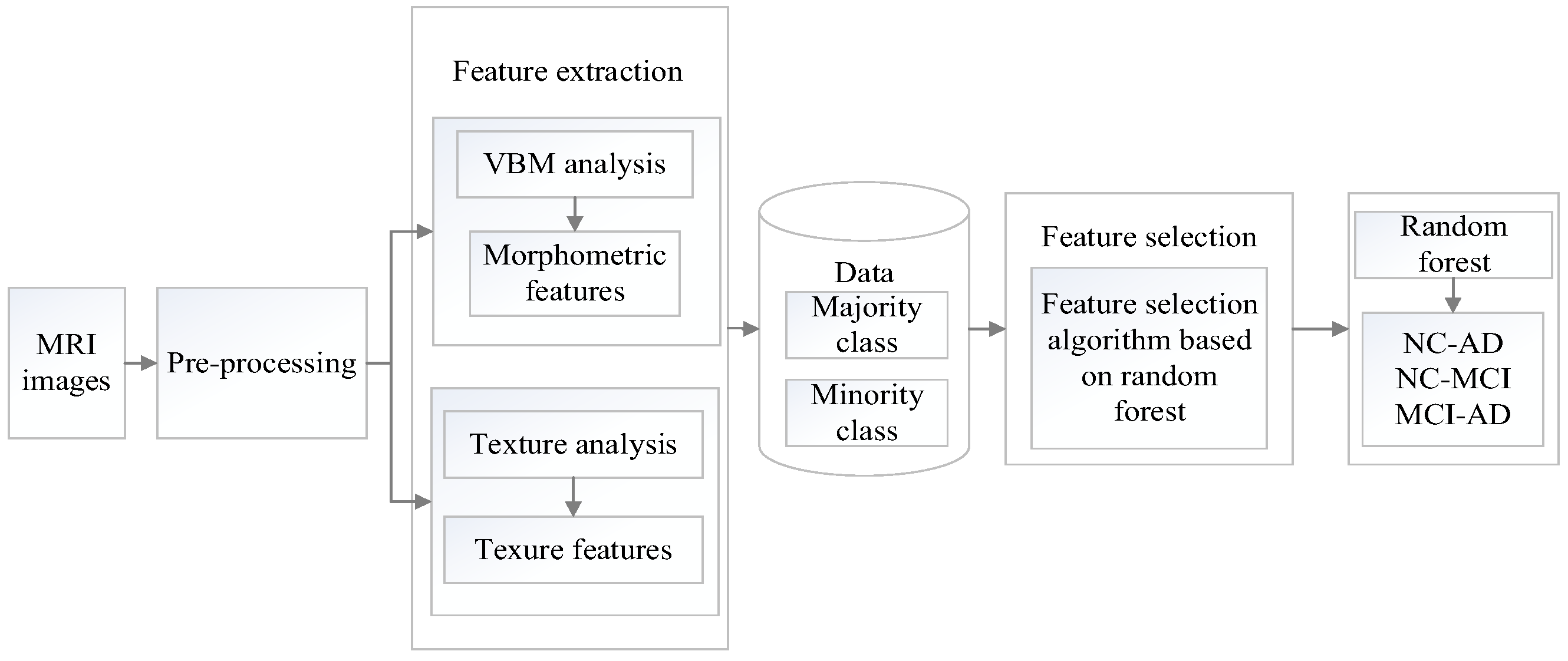
In this section, the proposed method will be described in detail. The overview of the proposed classification framework for imbalanced brain MRI image data is illustrated in Figure 1. The process is as follows: Firstly, collect MRI images from the ADNI database and conduct initial pre-processing such as gradient correction, non-uniformity correction, intensity unevenness correction, and scaling correction. Secondly, perform multi-type feature extraction and fusion. Thirdly, propose a new feature selection algorithm based on the random forest to obtain the optimal feature subset. Finally, classify images from the ADNI database by using classifiers.
In research on the current brain medical image feature extraction technologies, it can be found that the feature fusion method can retain more details of the image; therefore, this paper employs the feature fusion method to fuse the morphological features and texture features of the MRI images.
3.1. The Feature Extraction
3.1.1. Morphological Feature Extraction
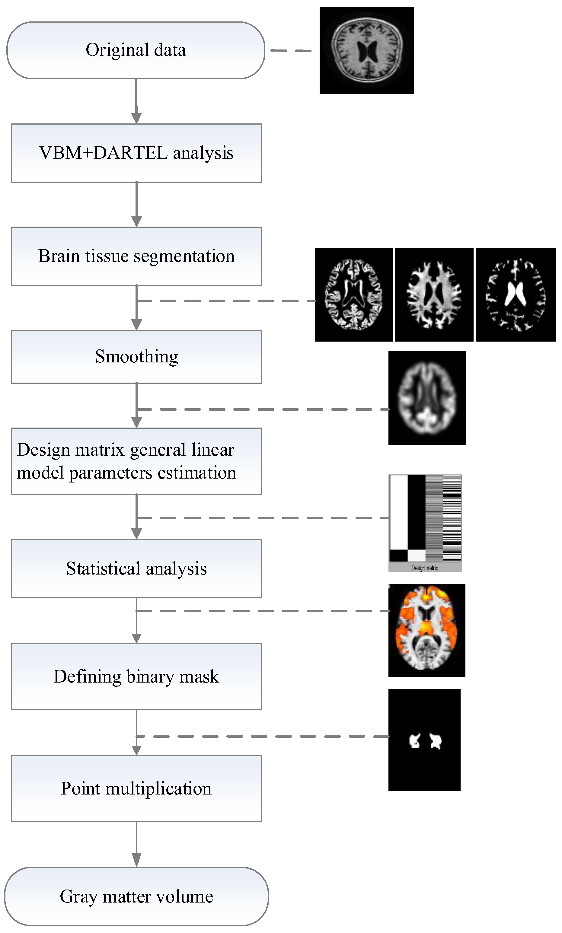
The VBM method is a voxel-based morphological measurement method that represents the morphological changes in brain tissue. Since it can estimate the density change of a certain voxel unit volume, it was employed to represent local brain features and brain tissue components. Baron et al. [54] used the VBM method to find that the total brain gray matter of people with AD was significantly reduced when compared with the normal elderly, which was consistent with the results obtained by the manual drawing method of [55] and the pathological results. Therefore, in this paper, ROI analysis of the MRI data was carried out using SPM8 software (http://www.fil.ion.ucl.ac.uk/spm, accessed on 10 September 2021) and the VBM8 toolbox (http://dbm.neuro.uni-jena.de/vbm, accessed on 10 September 2021). Furthermore, the gray matter volume of the lesion area was calculated as a morphological feature. Figure 2 illustrates the processing framework of morphological feature extraction.
The specific steps of morphological feature extraction are as follows:
Step 1: Space standardization. Images are processed by using the VBM–DARTEL algorithm, which not only improves the segmentation accuracy however additionally preserves the original volume information and ensures the accuracy of spatial standardization.
The VBM algorithm pre-segments the brain tissue, according to the prior probability information. In addition, it saves the volume of the medical image through modulation and uses the Jacobian determinant to store the volume change information of each pixel in the image, as shown in Formula (1):
In Formula (1), and represent the pixels before and after image registration, respectively. During the modulation process of the image, the volume information of the pixel is restored by multiplying the grayscale value of the pixel after image segmentation by the Jacobian matrix determinant of that pixel.
The DARTEL algorithm introduces a Lie algebra and flow field theory into the process of VBM space standardization and uses them to carry out nonlinear image registration, which compensates for the defects in the VBM algorithm registration process and improves the accuracy of registration. The principle of the DARTEL algorithm is as follows:
Firstly, assuming a constant flow field u; a differential equation describing the deformation field changing with time can be obtained through u, as shown in Formula (2):
A deformation field can be obtained by using Formula (2), where x is the position coordinate, representing the unit transformation, and the initial value of the time point . Formula (3) can be obtained by integrating over :
Further, use the Euler equation to transform Formula (2) and obtain Formula (4):
In Formula (4), h represents the time step, and different deformation fields Φ can be obtained by setting different time steps. The DARTEL algorithm obtains the corresponding deformation field by exponentiating the flow field, which ensures that the determinant of the Jacobian matrix is always positive while obtaining the deformation field so that the registration result is diffeomorphic;
Step 2: Brain tissue segmentation. After the processing of spatial normalization, the images are segmented into gray matter (GM), white matter (WM), and cerebrospinal fluid (CSF);
Step 3: Spatial smoothing. Spatial smoothing is a filtering process, based on images of the different tissue in segments. In this process, a Gaussian kernel function is used to convolve image data in the standard space. The purpose of the smoothing is to eliminate subtle matching errors and improve the signal-to-noise ratio;
Step 4: Defining ROI binary image. At present, VBM statistical analysis is based on a generalized linear model. It performs a two-sample t-test on the hypothesis to detect whether there is a significant difference in the density of certain regions of the gray matter images between the two groups. The gray matter density regions with significant differences are identified as an area of interest.
The two-sample t-test was used to analyze whether there are significant differences between the brain medical image data of normal people and those with AD lesions and to identify the brain regions with more serious differences. The process is as follows:
Original hypothesis H0: assume that the population means values of the 2 samples are equal.
Alternative Hypothesis H1: assume that the population means values of the 2 samples are not equal.
The t-value is calculated in the 2-sample statistical test as shown in Formula (5):
In Formula (5), and represent the population means values of the 2 independent samples, respectively. The solution of is shown in Formula (6):
In Formula (6), and represent their sample variances, respectively, and their calculation methods are shown in Formulas (7) and (8).
where n1 and n2 represent the total numbers of sample 1 and sample 2, respectively.
In the case of a certain significance level, according to the t critical value table, if t is greater than the critical threshold, then the result is to reject H0 and accept H1, which proves that there is a significant difference between the 2 sample populations.
A two-sample t-test was performed on different groups of AD brain medical image data by VBM to detect the regions where they have significant differences;
Step 5: Gray matter volume calculation. After VBM analysis, the ROI of the lesion area was obtained. The ROI binary masks were made by using the WFU_PickAtlas (https://www.nitrc.org/projects/wfu_pickatls, accessed on 10 September 2021). Because the two MRI images for dot product calculation must have the same dimension, the ROI binary masks additionally needed to be resampled to have the same dimensions as the gray matter image. Then the resampled ROI binary mask and the gray matter image were implemented in the dot product calculation to obtain a gray matter volume.
3.1.2. Texture Feature Extraction
We extracted various texture features, based on the Gray-Level Co-occurrence Matrix and Gray-Gradient Co-occurrence Matrix techniques. The specific steps for texture feature extraction are as follows:
Step 1: Gray-level co-occurrence matrix. The gray-level co-occurrence matrix reflects the comprehensive information on the gray level of the image concerning direction, adjacent spacing, and variation amplitude. It is the basis of analyzing the local patterns of images and their permutation rules. Therefore, we can extract a series of features to describe the image. The texture feature extraction method was proposed by [12,56,57], which provides us with a calculation and theoretical basis. In this paper, the selected spatial distance is from 1 to 6 pixels, and the directions are 0°, 45°, 90°, and 135°. A total of 24 gray-level co-occurrence matrices were constructed, and 12 features were employed, including angular second moment, variance, inverse difference moment, sum averages, sum variances, contrast, entropy, correlation, difference averages, sum entropy, difference entropies, and difference variance;
Step 2: Gray-gradient co-occurrence matrix. The gray-gradient co-occurrence matrix reflects the relationship between the gray level and the gradient (or edge) of the pixel in the image [58]. The gray level of each image point is the basis of the image, and the gradient is the element that constitutes the edge contour of the image. The main information of the image is provided by the edge contour. In this paper, 15 features were employed, including small gradient advantage, large gradient advantage, gray distribution inhomogeneity, gradient distribution inhomogeneity, energy, gray average, gradient average, gray mean square variance, gradient mean square variance, correlation, gray entropy, gradient entropy, mixed entropy, inertia, and inverse difference moment.
3.2. The Proposed RF–AUC–Cor Algorithm
After the feature extraction, the extracted morphological features and texture features were combined linearly to obtain feature data. Unfortunately, there are some redundant, irrelevant, and less effective features among them, which will impact the effect of classification prediction. Moreover, the data we studied are imbalanced. Therefore, traditional feature selection algorithms are usually limited by the classification target of the highest accuracy, such that the final selected features tend to classify the minority class into the majority class. However, the minority class is what we most want to identify. Therefore, we propose a random forest-based feature selection algorithm, called RF–AUC–Cor, for high dimensional imbalanced data. The algorithm can alleviate the problem of imbalanced distribution, while performing feature selection and treating the features of the majority class and minority class fairly. The specific description of the RF–AUC–Cor algorithm is as follows:
- (1)
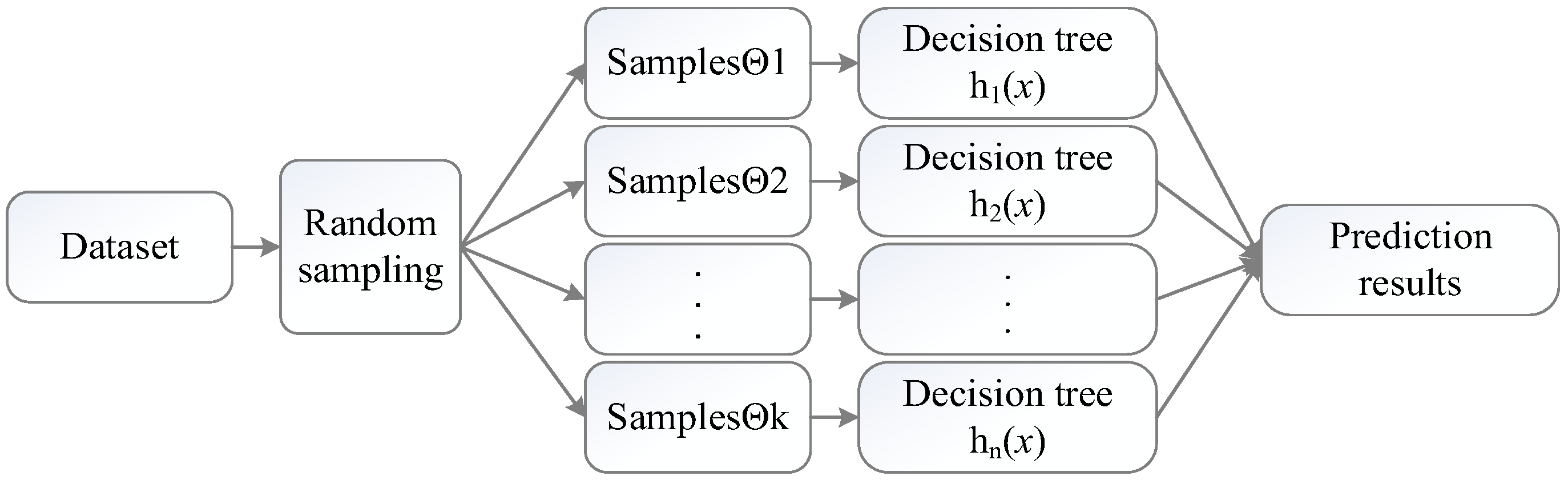
- Random Forest. The random forest is a decision tree integration algorithm proposed by [59]. For a given x vector, each decision tree has the right to vote and finally summarizes the voting results. The class of x is determined, based on the principle of the minority obeying the majority.
The structure of the random forest algorithm is shown in Figure 3.
In Figure 3, the random forest obtains a combination of base classifiers, including after k training, and an ensemble classifier is formed by the base classifier. The base classifier generates the final predicted result by voting. Afterward, the random forest algorithm summarizes the voting results of all base classifiers, and the result with the highest score is used as the final prediction result. The voting calculation method is shown in Formula (9):
where H(x) is the combination classification model, hk is a decision tree model, y represents the decision tree classification result, and I(·) is an indicator function.
To sum up, the random forest obtains the decision tree model based on training samples, then uses the branch nodes of the decision tree to compare the eigenvalues of the test set, and finally completes the class judgment at the leaf nodes. Compared to other classifiers, random forests have a superior effect on both accuracy and AUC. Therefore, we choose the random forest to evaluate each feature;
- (2)
- AUC evaluation criteria. For the problem of data imbalance, accuracy is not a good criterion for classification performance. For example, if the ratio of majority class to minority class of the imbalanced data is 9:1, then even if all the minority classes are misclassified into the majority class the final accuracy can reach 90%; however, the cost of this misclassification is very high. Therefore, researchers introduced several new performance criteria for imbalanced data problems. The most widely used criterion is the AUC. Because the AUC can treat the majority class and minority class fairly and our goal is to improve the AUC of diagnosis and prediction by feature selection, we use AUC as the evaluation criteria for the feature selection of the AD data;
- (3)
- Correlation analysis. The correlation matrix provides the correlation analysis between two sets of observed variables. Taking 2 random variables X and Y as examples, and allowing n to be the number of 2 variables, then the correlation is calculated as follows:
The correlation matrix reflects the correlation between two observation variables. The elements of the ith row and the jth column of the correlation matrix are the correlation coefficients of the ith column and the jth column of the original matrix, which corresponds to the degree of redundancy between the corresponding variables;
- (4)
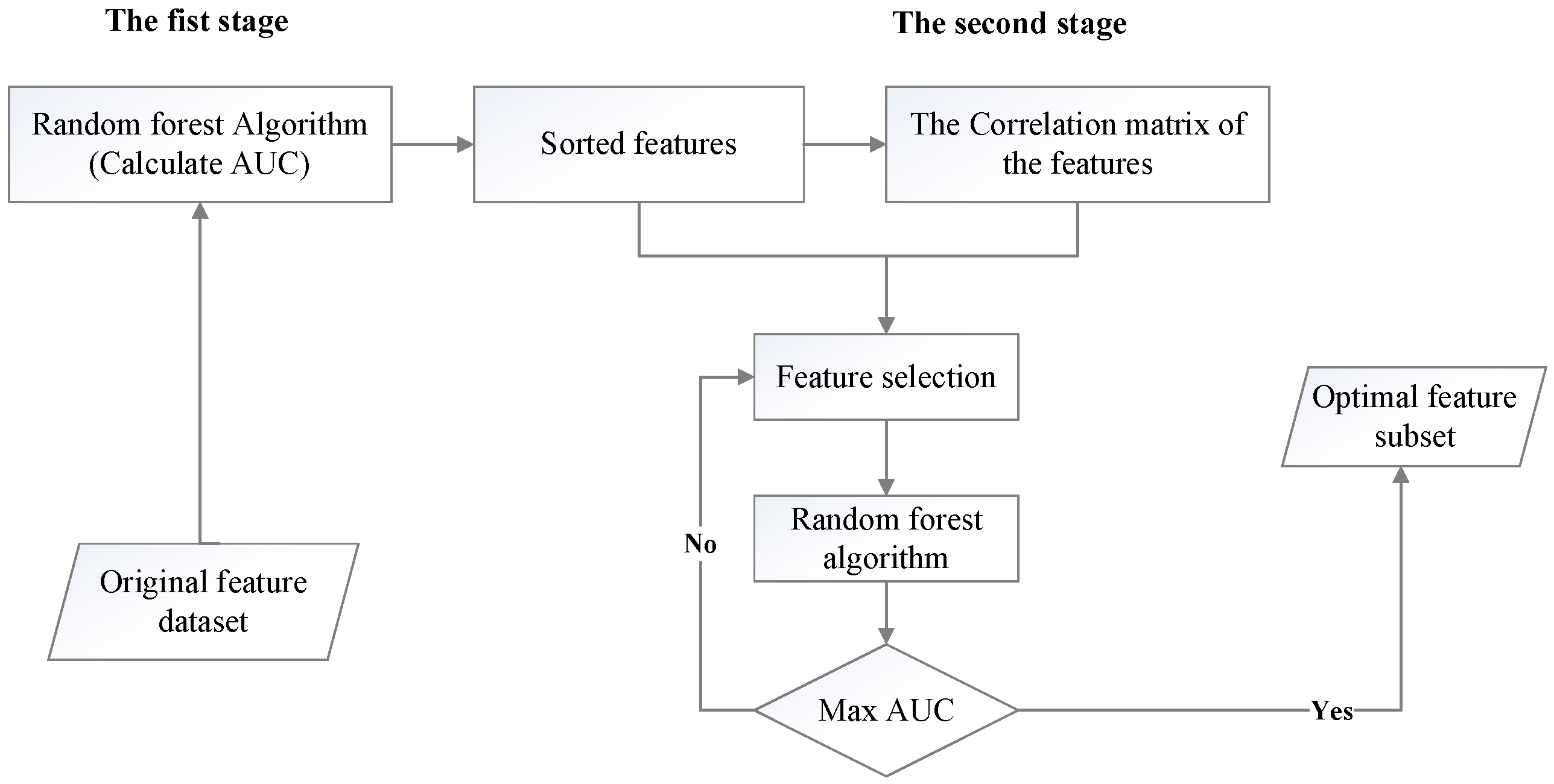
- RF–AUC–Cor algorithm. To optimize the process of feature selection, the RF–AUC–Cor algorithm is proposed in this paper, as shown in Figure 4. The procedure of the RF–AUC–Cor algorithm is divided into two steps. In the first step, the random forest is used to classify samples when evaluating the features. The AUC of each feature is calculated, and the features are sorted in descending order based on their AUC values. In the second step, the correlation between all features is calculated. Moreover, according to the correlation matrix and the sorted features, the feature subsets are generated by feature selection. Finally, the random forest is used to verify the feature subset.
The specific process of the RF–AUC–Cor algorithm is as follows:
Step 1: Utilize random forest to classify samples, calculate the AUC value of each feature, sort the features by AUC value as the score, and obtain a new sorted feature set;
Step 2: For the sorted feature set, calculate the correlation between the features and obtain the correlation matrix;
Step 3: The initial state of the subset is empty, and in the process of selecting the feature subset, one feature is selected to add to the existing feature subset each time. The selected feature is the feature with the highest score in the feature ranked set, or the feature which has the minimal redundancy with the highest score feature that was selected last time;
Step 4: Based on the above analysis, in the feature selection process it is necessary to determine whether to continuously select the K highest ranked features, or the consecutive K features that have the minimum redundancy with the highest score feature that was selected last time;
Step 5: Each selection obtains a new feature subset, and the random forest is employed to classify the samples. The feature subset with the highest AUC value is the optimal feature subset to be selected.
4. Results and Analysis
4.1. Experimental Dataset
The data used in our experiments come from the large ADNI public database of the United States. The sample image is a weighted MRI, with a magnetic flux of 1.5. The number of samples is 602, including 50 AD cases, 332 NC cases, and 220 MCI cases. The description of the data information is shown in Table 1, which lists the numbers, ages, simple mental state table (MMSE), and clinical dementia rating (CDR) of AD, NC, and MCI, respectively. The total score of MMSE is 30 points. It evaluates scores according to the educational level. If the score is below the cut-off value, it is a functional defect, and a score above the cut-off value is normal: illiterate (uneducated) is 17 points, primary school (education years ≤ 6 years) is 20 points, and secondary school or above (education years ≥ 6 years) is 24 points. CDR is used to assess the severity of dementia: healthy (CDR = 0), suspected dementia (CDR = 0.5), mild dementia (CDR = 1), moderate dementia (CDR = 2), and severe dementia (CDR = 3).
The information on features is shown in Table 2. For the NC–AD group data, the total number of features is 312, including 303 texture features and 9 morphological features. For the NC–MCI group data, the total number of features is 314, including 303 texture features and 11 morphological features. For the MCI–AD group data, the total number of features is 316, including 303 texture features and 13 morphological features. This paper mainly studies the binary classification problem. In the actual diagnosis process, it is not only necessary to identify the patients from normal people however additionally to consider the degree of disease. After all, MCI in the later stage is easily confused with AD. Therefore, we additionally need to consider the distinction between MCI and AD.
4.2. Experimental Setup
The experiments performed in this study aimed to minimize bias with the use of randomness and generate a classification model with relative stability. Subsequently, the preprocessed data were divided into majority and minority sub-datasets. Further, 10-fold cross-validation was used to evaluate the classification model. The training and testing sets from each class were combined to generate a training dataset and a testing dataset. The dataset was divided into 10 parts: 9 parts were randomly selected as training samples to build a classification model, and the other part was used as a test set to test the model’s performance. After each training model, the training and testing accuracy rates were obtained and repeated 5 times, and the average of the 5 training and testing results were taken as the final classification accuracy rate of the model. Given the imbalance of data distribution, in addition to classification accuracy, AUC is additionally considered an evaluation criterion of classifier performance.
The calculation method of classification accuracy is shown in Formula (11):
where TP (true positives) represents the number of correctly identified positive cases in the classification results; FP (false positives) represents the number of cases that are incorrectly identified as positive cases in the classification results; FN (false negatives) represents the number of cases that are incorrectly identified as negative in the classification results; and TN (true negatives) represents the number of correctly identified negative cases in the classification results.
Since AUC is the area enclosed by the ROC curve and the coordinate axis, the AUC value can be obtained by calculating the points on the ROC curve, so it can reflect the changing trend of the ROC curve.
(1) Calculate the area directly from the ROC curve. Assuming that there are m points on the ROC curve, which are formed by the classification results obtained by classifier training, where x1, x2,…, xm represent the abscissas of these points and y1, y2,…, ym represent the ordinates, then the AUC value can be calculated using Formula (12):
(2) Calculate the equivalent of AUC using the error rate, supposing that X is the sample dataset to be predicted, which consists of m majority class samples and n minority class samples. After training the classifier samples, all prediction results are given. In the statistical prediction results, the number of misclassified minority class samples into majority class samples is x, and the number of majority class samples misclassified into minority class samples is y. Calculating the AUC value of the classifier is shown in Formula (13):
4.3. Experimental Results and Evaluation
In this section, three experiments are conducted to compare and analyze the performance of the algorithm. The first step is to verify the effect of the parameter K (see the proposed RF–AUC–Cor algorithm in Section 3.1.2) on the proposed algorithm. The second is to evaluate alternative feature selection algorithms. The third is to compare the distinct classification models.
4.3.1. The Effect of the Parameter K on the Proposed Algorithm
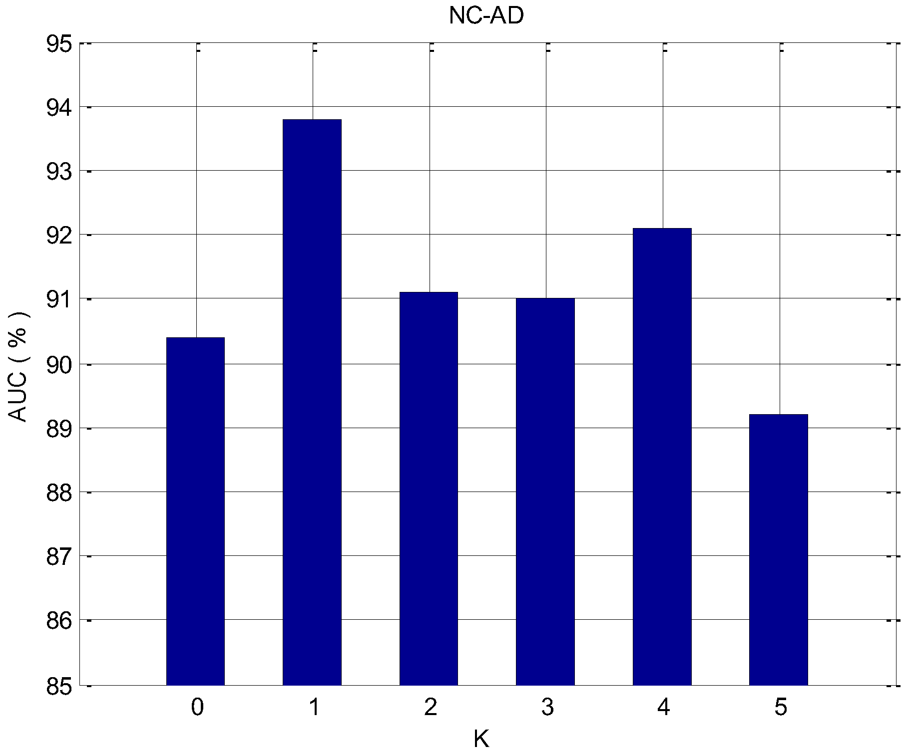
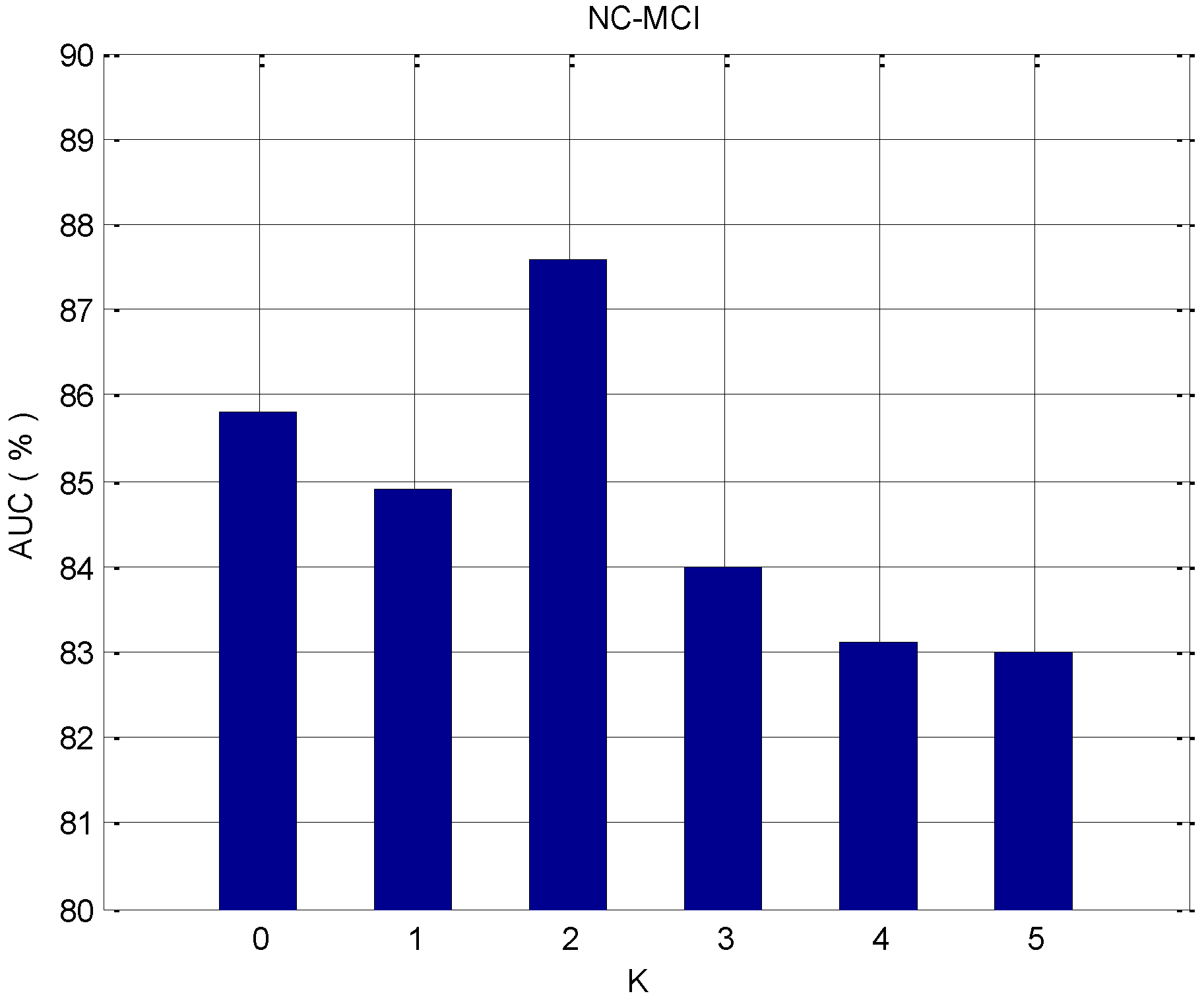
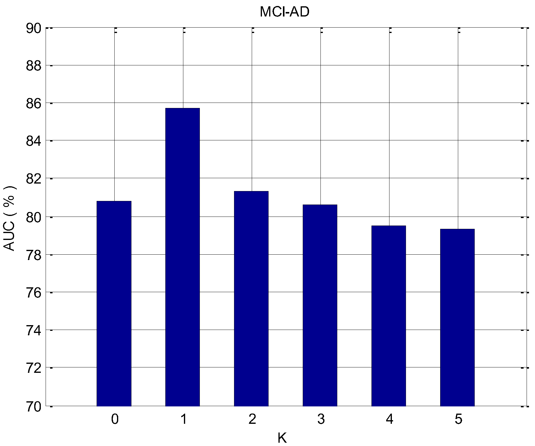
To prove the validity of the proposed feature selection algorithm, we applied it to the data of NC–AD, NC–MCI, and MCI–AD, respectively. In the feature selection process, it is necessary to determine whether to continuously select the K with the highest ranked features, or the consecutive K features that have the minimum redundancy with the highest score feature that was selected last time. For each dataset, the influence of different parameters K on the classification effect is analyzed. For the classification problem of imbalanced data, the accuracy cannot evaluate the effect of the classifier well, and the AUC is the more important evaluation criterion. Thus, we evaluate the effect of the algorithm by considering the AUC value. Figure 5, Figure 6 and Figure 7 depict the change of the AUC by using the random forest classification prediction under a different K.
K represents the number of features that need to be selected in the feature selection process and have the minimum redundancy with the previous highest-ranked feature. When K equals 0, the redundancy among features is not considered. Features are sorted by the AUC and added to the feature subset each time, and the top K features are finally selected as the feature subset. When the value of K becomes larger and affected by the redundancy between features, the classification performance will be affected. For the NC–AD group data, when K equals 1, the classification performance is maximized, and the maximum value is 93.7%. In the case of the NC–MCI group data, when K equals 2, the classification performance is maximized, and the maximum value is 87.6%. For the MCI–AD group data, when K equals 1, the classification performance is maximized, and the maximum value is 85.7%. For these three datasets, when we observe the results at the overall level, it can be seen clearly that when K becomes larger and reaches a certain value, the classification performance will decrease. This is because as K increases, the redundancy between features is over-considered, and the importance of the features themselves may be ignored.
4.3.2. Compared with Other Feature Selection Algorithms
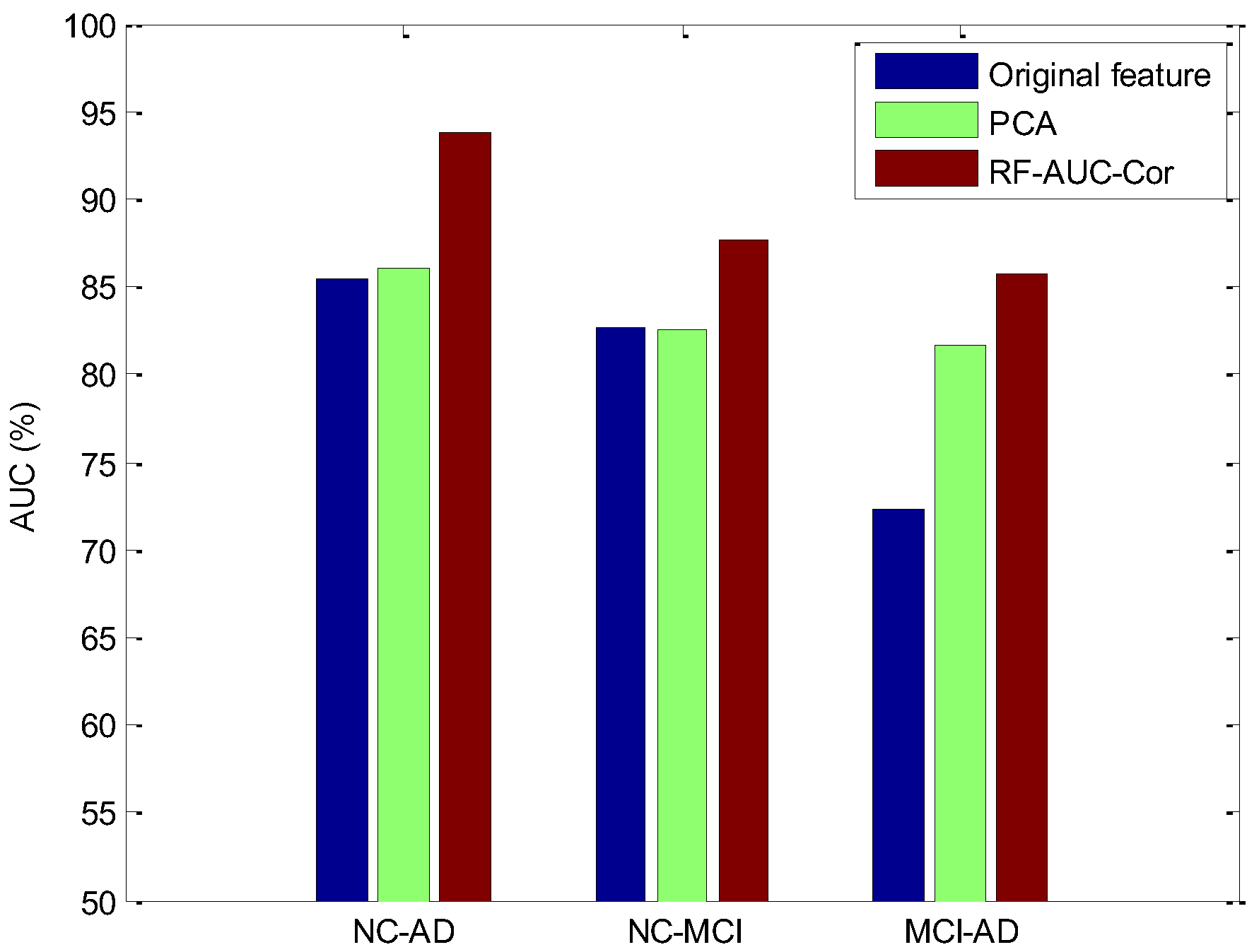
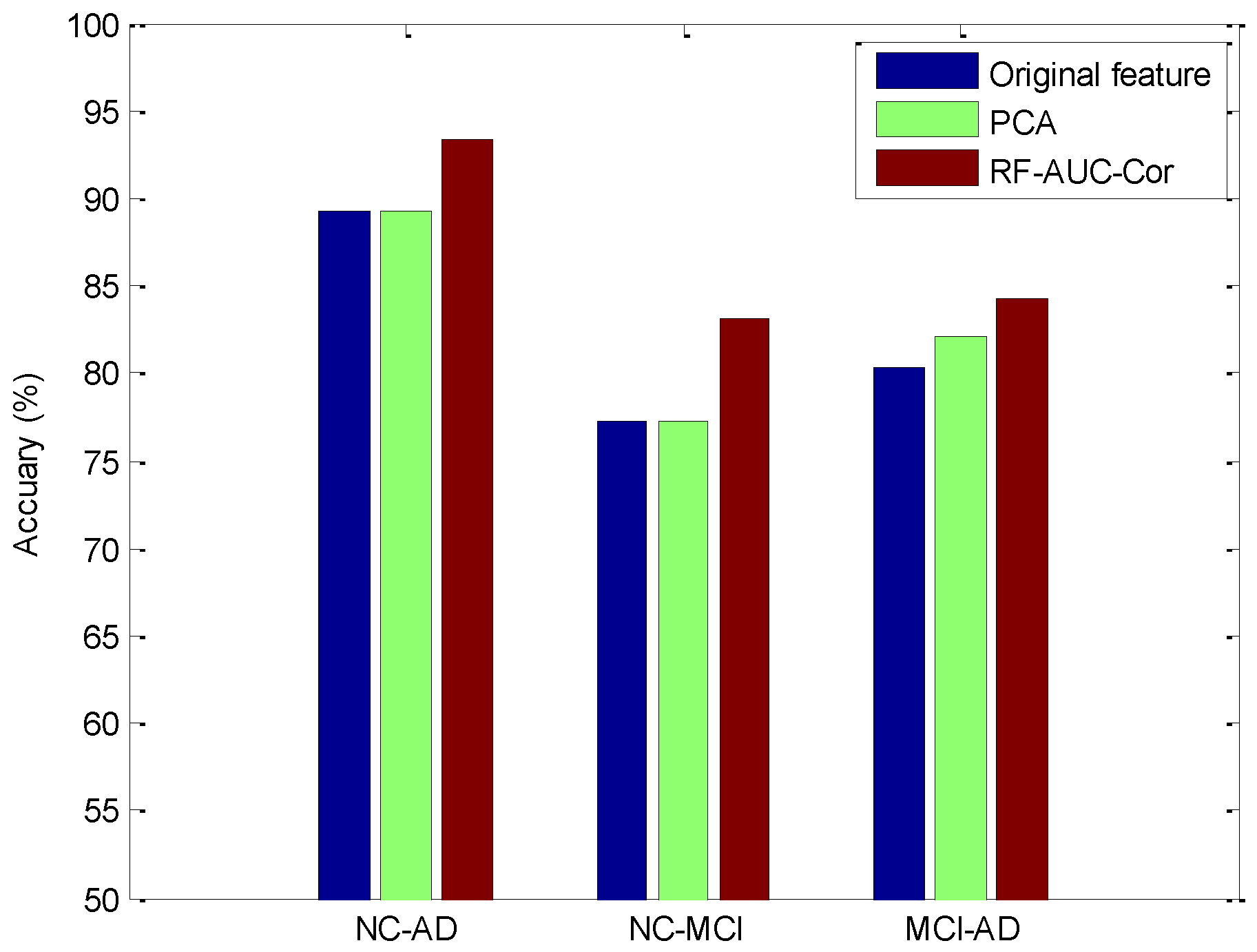
Based on the above experimental results, we can find that when K equals 1, the NC–AD and the MCI–AD groups’ data obtain the optimal feature subset. While K equals 2, the NC–MCI group data obtain the optimal feature subset. To prove the effectiveness of the RF–AUC–Cor algorithm proposed in this paper, we evaluated with two other strategies. One is the classification schema without feature selection, and the other is the classification schema using the PCA (principal components analysis) dimensionality reduction technology. PCA is one of the most widely used dimension reduction algorithms, and its performance has been proven in many of the literatures. The experimental results are the average classification results of 10-fold cross-validation, which are presented in Figure 8 and Figure 9.
From Figure 8 and Figure 9, it can be found that the proposed method achieved a superior AUC and accuracy than the PCA method, and the superiority is significantly relevant in the NC–AD group data, which proves that the random forest base RF–AUC–Cor feature selection algorithm is effective in high dimensional imbalanced data scenarios. Consequently, the algorithm proposed in this paper not only improves the recognition rate of the minority class however additionally guarantees a higher accuracy rate.
4.3.3. Compared with Other Classification Models
In this section, we compare the performance of our model with state-of-the-art methods, including SVM [60,61], RNN [62], CNN [63], and KNN (RFE + PCA) [52]. In [61], the importance-based feature selection was adopted, and an SVM-based AD classification model was further established. Glozman et al. [61] developed shape descriptors to capture and quantify these changes and test their efficacy as imaging biomarkers for the automatic classification of the following populations: MCI patients who progressed to AD, AD patients, and normal controls (NC). Qasim et al. [52] proposed a KNN model, based on RFE and PCA to identify AD, which used RFE and PCA for feature selection. Ghazi et al. [62] and Rana et al. [63] utilized different deep neural works for AD classification. In our study, the examination was conducted by splitting the data into 90–10 in the train-test split approach, and the experimental results are shown in Table 3.
Table 3 presents the overall performance of the six methods. Since ADNI is an imbalanced dataset, from the experimental results and the data preprocessing method adopted, it can be found that designing an appropriate feature selection strategy for the characteristics of the dataset can effectively improve the performance of the model. For example, comparing the first and second methods in Table 3, the second method designs a more scientific feature selection algorithm, and therefore, its classification performance is better than the first method. For the second and third methods, regarding the NC–AD classification problem, the third method designs a more reasonable feature selection algorithm, in which RFE is applied with PCA to reduce the number of features; therefore, its performance is significantly better than the second method. Theoretically speaking, the fourth and fifth methods should obtain higher classification accuracy and AUC values compared with other methods; however, the experimental results are just the opposite. The main reason for this is closely related to the imbalance of the dataset and the quality of the learned features. The performance of the method proposed in this paper is significantly better than other methods for the NC–AD classification problem; regarding the MCI–AD classification problem, its comprehensive performance (including classification accuracy, the AUC, and training time) can be ranked first. In this study, morphological features and texture features were extracted and fused, and feature selection was additionally applied to the dataset as a preprocessing step. On the one hand, it can reduce the classification performance degradation caused by data imbalance; on the other hand, it can additionally reduce the time complexity of model training. Moreover, the classification performance results of all the models were comprehensively discussed. Therefore, the proposed AD diagnostic method can help medical practitioners efficiently identify patients with AD.
4.3.4. Discussion
Based on MRI, the early lesion features of NC and MCI can be detected, and many studies have extracted brain features for the classification of NC, AD, and MCI. However, in the classification process, the class imbalance problem seriously affects the classification effect. Drawing on the existing solutions, this paper proposed a new feature extraction and fusion method to solve this problem. Meanwhile, considering the redundancy between the extracted features and further feature selection, only the key features that have a significant impact on the disease are screened out. In this way, the dimension of input features can be effectively reduced, the time cost of model training can be cut, and the classification prediction effect is better. Furthermore, the main factors affecting diagnosis can be found, and a reference for clinical practice can be provided.
In the experiments with the feature extraction, firstly, the effect of the parameter K on the proposed algorithm was verified and then compared with other feature extraction methods, including PCA (in Section 4.3.2) and RFE + PCA (in Section 4.3.3). The results indicate that the proposed method can identify the minority class samples well and avoid the unsatisfactory classification effect caused by the majority class. This is similar to integrating oversampling technology and undersampling technology to preprocess samples. Therefore, the method proposed in this paper can deal well with the problem of unsatisfactory classification results caused by class imbalance.
In our study, we have demonstrated that the random forest model can take MRI features and accurately predict NC–MCI, NC–AD, and MCI–AD problems. Our proposed classifier showed a superior performance compared to the competing SVM, KNN, RNN, and CNN. It is worth noting that this model has the highest accuracy and AUC value for the NC–AD group data (94.2% and 93.7%) classification problem, followed by MCI–AD (84.5% and 85.7%) and NC–MCI group data (83.8% and 87.6%) classification problems. Moreover, the training time of our model is the shortest, which is far lower than other models, of approximately 3.0 s only. Therefore, the proposed method can well predict the progression of disease from NC to AD, from MCI to AD, and from NC to MCI, which is critical to the study of why only certain NC and MCI patients develop AD, as well as to understanding the disease and developing accurate prognostic indicators.
Furthermore, our original intention is to apply the proposed preprocessing method for class-imbalanced datasets to the whole field of medical research. Since most medical datasets contain a similar target class imbalance, our approach incorporates multi-type features to balance the weight of the minority class in the model. Currently, the proposed approach was only tested on binary classification problems; we plan to apply it to multi-class classification problems as well.
One limitation of this study is that all patients were from the ADNI dataset. Although we split the dataset into multiple instances to validate its accuracy and AUC, no participant populations other than ADNI were tested. Taking other datasets as test objects for the model will be more helpful to verify its effectiveness, which is the goal of our future work.
5. Conclusions and Future Work
In this paper, we proposed an effective classification framework to effectively identify imbalanced Alzheimer’s disease (AD), mild cognitive impairment (MCI), and normal control (NC). Firstly, we extracted the features of AD, MCI, and NC, and then extracted and linearly combined morphological features and texture features as feature data. Secondly, based on the high dimensional imbalance characteristics of the data, we proposed the feature selection approach RF–AUC–Cor, which not only evaluates the imbalance of data however additionally estimates the redundancy between features. The experimental results showed that the RF–AUC–Cor algorithm has some practical application value and can effectively reduce the misclassification rate of minority data instances.
In future work, we intend to address the following aspects: First, we will continue to increase the number of samples and the diversity of the samples, and then we will investigate the algorithm’s performance on new datasets. Second, based on the characteristics of the class-imbalanced datasets, we will examine additional pre-processing methods, evaluate the performance indicators for each method, and then apply these methods to actual projects. In addition, we will consolidate the study of the current project, annotate the disease dataset, and create a knowledge graph for researchers to study collaboratively.
Author Contributions
Conceptualization, X.W., Q.Z., H.L. and M.C.; methodology, X.W. and Q.Z.; software, X.W. and Q.Z.; validation, H.L. and M.C.; formal analysis, X.W. and Q.Z.; investigation, X.W., Q.Z., H.L. and M.C.; resources, H.L., X.W. and M.C.; data curation, H.L. and X.W.; writing—original draft preparation, Q.Z. and X.W.; writing—review and editing, H.L. and M.C.; visualization, Q.Z. and X.W.; project administration, X.W. and H.L.; funding acquisition, X.W. and H.L. All authors have read and agreed to the published version of the manuscript.
Funding
This work was partially supported by the National Natural Science Foundation of China (grant nos. 72161005, 62162010, 71901078, and 71964009), Research Projects of the Science and Technology Plan of Guizhou Province (grant nos. QianKeHeJiChu-ZK [2022] General 184, [2021] 449, [2023] 010, [2023] 276), High-Level Talent Project of Guizhou Institute of Technology (grant no. XJGC20190929), and Special Key Laboratory of Artificial Intelligence and Intelligent Control of Guizhou Province (grant no. KY [2020]001).
Institutional Review Board Statement
Not applicable.
Informed Consent Statement
Not applicable.
Data Availability Statement
The ADNI dataset used to support the findings of this study is available at https://adni.loni.usc.edu/ (accessed on 21 September 2021).
Acknowledgments
The authors would like to thank the Guizhou Engineer Lab of ACMIS for their support.
Conflicts of Interest
The authors declare no conflict of interest.
References
- Wilson, R.S.; Segawa, E.; Boyle, P.A.; Anagnos, S.E.; Hizel, L.P.; Bennett, D.A. The natural history of cognitive decline in Alzheimer’s disease. Psychol. Aging 2012, 27, 1008–1017. [Google Scholar] [CrossRef] [Green Version]
- Patterson, C. World Alzheimer Report 2018; Alzheimer’s Disease International: London, UK, 2018. [Google Scholar]
- Alzheimer’s Association. 2015 Alzheimer’s disease facts and figures. Alzheimer’s Dement. 2015, 11, 332–384. [Google Scholar] [CrossRef] [PubMed]
- Ronald, R.C.; Smith, G.E.; Waring, S.C.; Ivnik, R.J.; Tangalos, E.G.; Kokmen, E. Mild cognitive impairment: Clinical characterization and outcome. Arch. Neurol. 1999, 56, 303–308. [Google Scholar]
- Reitz, C.; Mayeux, R. Alzheimer disease: Epidemiology, diagnostic criteria, risk factors and biomarkers. Biochem. Pharmacol. 2014, 88, 640–651. [Google Scholar] [CrossRef] [PubMed] [Green Version]
- Colloby, S.J.; Taylor, J.P. Patterns of cerebellar volume loss in dementia with lewy bodies and Alzheimer’s disease: A VBM-DARTEL study. Psychiatry Res. Neuroimaging 2014, 223, 187–191. [Google Scholar] [CrossRef] [Green Version]
- Zhang, F.; Tian, S.; Chen, S.; Ma, Y.; Li, X.; Guo, X. Voxel-based morphometry: Improving the diagnosis of Alzheimer’s disease based on an extreme learning machine method from the ADNI cohort. Neuroscience 2019, 414, 273–279. [Google Scholar] [CrossRef] [PubMed]
- Jack, C.R., Jr.; Wiste, H.J.; Schwarz, C.G.; Lowe, V.J.; Senjem, M.L.; Vemuri, P.; Petersen, R.C. Longitudinal tau PET in ageing and Alzheimer’s disease. Brain 2018, 141, 1517–1528. [Google Scholar] [CrossRef] [PubMed] [Green Version]
- Busatto, G.F.; Diniz, B.S.; Zanetti, M.V. Voxel-based morphometry in Alzheimer’s disease. Expert Rev. Neurother. 2008, 8, 1691–1702. [Google Scholar] [CrossRef]
- Ashburner, J.; Friston, K.J. Voxel-based morphometry-the methods. Neuroimage 2000, 11, 805–821. [Google Scholar] [CrossRef] [Green Version]
- Guo, Y.; Zhang, Z.; Zhou, B.; Wang, P.; Yao, H.; An, N.; Dai, H.; Wang, L.; Zhang, X. Grey-matter volume as a potential feature for the classification of Alzheimer’s disease and mild cognitive impairment: An exploratory study. Neurosci. Bull. 2014, 30, 477–489. [Google Scholar] [CrossRef] [Green Version]
- Humeau-Heurtier, A. Texture feature extraction methods: A survey. IEEE Access 2019, 7, 8975–9000. [Google Scholar] [CrossRef]
- Zaletel, I.; Milutinović, K.; Bajčetić, M.; Nowakowski, R.S. Differentiation of Amyloid Plaques Between Alzheimer’s Disease and Non-Alzheimer’s Disease Individuals Based on Gray-Level Co-occurrence Matrix Texture Analysis. Microsc. Microanal. 2021, 27, 1146–1153. [Google Scholar] [CrossRef]
- Mathew, A.R.; Anto, P.B. Tumor detection and classification of MRI brain image using wavelet transform and SVM. In Proceedings of the 2017 International Conference on Signal Processing and Communication (ICSPC), Coimbatore, India, 28–29 July 2017; IEEE: Piscataway, NJ, USA, 2017; pp. 75–78. [Google Scholar]
- Li, Y.; Hsu, W.W.; Alzheimer’s Disease Neuroimaging Initiative. A classification for complex imbalanced data in disease screening and early diagnosis. Stat. Med. 2022, 41, 3679–3695. [Google Scholar] [CrossRef]
- Estabrooks, A. A Combination Scheme for Inductive Learning from Imbalanced Data Sets. MCS Thesis, Faculty of Computer Science, Dalhousie University, Halifax, NS, Canada, 2000. [Google Scholar]
- Taieb, J.; Svrcek, M.; Cohen, R.; Basile, D.; Tougeron, D.; Phelip, J. Deficient mismatch repair/microsatellite unstable colorectal cancer: Diagnosis, prognosis and treatment. Eur. J. Cancer 2022, 175, 136–157. [Google Scholar] [CrossRef]
- Wu, Y.L.; Wu, F.; Xu, C.P.; Chen, G.L.; Zhang, Y.; Chen, W.; Yan, X.C.; Duan, G.J. Mediastinal follicular dendritic cell sarcoma: A rare, potentially under-recognized, and often misdiagnosed disease. Diagn. Pathol. 2019, 14, 1–11. [Google Scholar] [CrossRef]
- Li, J.; Fong, S.; Liu, L.; Dey, N.; Ashour, A.S.; Moraru, L. Dual feature selection and rebalancing strategy using metaheuristic optimization algorithms in X-ray image datasets. Multimed. Tools Appl. 2019, 78, 20913–20933. [Google Scholar] [CrossRef]
- Xiao, Z.; Ding, Y.; Lan, T.; Zhang, C.; Luo, C.; Qin, Z. Brain MR Image Classification for Alzheimer’s Disease Diagnosis Based on Multifeature Fusion. Comput. Math. Methods Med. 2017, 2017, 1952373. [Google Scholar] [CrossRef] [PubMed] [Green Version]
- Shankar, V.G.; Sisodia, D.S.; Chandrakar, P. A novel discriminant feature selection–based mutual information extraction from MR brain images for Alzheimer’s stages detection and prediction. Int. J. Imaging Syst. Technol. 2022, 32, 1172–1191. [Google Scholar] [CrossRef]
- Baskar, D.; Jayanthi, V.S.; Jayanthi, A.N. An efficient classification approach for detection of Alzheimer’s disease from biomedical imaging modalities. Mulitimed. Tools Appl. 2019, 78, 12883–12915. [Google Scholar] [CrossRef]
- Richhariya, B.; Tanveer, M.; Rashid, A.H. Diagnosis of Alzheimer’s disease using universum support vector machine based recursive feature elimination (USVM-RFE). Biomed. Signal Proces. 2020, 59, 101903. [Google Scholar] [CrossRef]
- Feng, J. Extracting ROI-Based Contourlet Subband Energy Feature from the sMRI Image for Alzheimer’s Disease Classification. IEEE/ACM Trans. Comput. Biol. Bioinform. 2021, 19, 1627–1639. [Google Scholar] [CrossRef] [PubMed]
- Liu, J.; Pan, Y.; Wu, F.X.; Wang, J.X. Enhancing the feature representation of multi-modal MRI data by combining multi-view information for MCI classification. Neurocomputing 2020, 400, 322–332. [Google Scholar] [CrossRef]
- Lao, H.; Zhang, X.; Tang, Y. Alzheimer’s disease diagnosis based on the visual attention model and equal-distance ring shape context features. IET Image Process. 2021, 15, 2351–2362. [Google Scholar] [CrossRef]
- Ansingkar, N.P.; Patil, R.; Deshmukh, P.D. An efficient multi class Alzheimer detection using hybrid equilibrium optimizer with capsule auto encoder. Multimed. Tools Appl. 2022, 81, 6539–6570. [Google Scholar] [CrossRef]
- Xu, C.; Xu, L.; Gao, Z.; Zhao, S.; Zhang, H.; Zhang, Y.; Du, X.; Zhao, S.; Ghista, D.; Liu, H.; et al. Direct delineation of myocardial infarction without contrast agents using a joint motion feature learning architecture. Med. Image Anal. 2018, 50, 82–94. [Google Scholar] [CrossRef] [PubMed]
- Rao, A.; Park, J.; Woo, S.; Lee, J.Y.; Aalami, O. Studying the effects of self-attention for medical image analysis. In Proceedings of the IEEE/CVF International Conference on Computer Vision (ICCV) Workshops, Virtual, 11–17 October 2021; pp. 3416–3425. [Google Scholar]
- Cai, Y.; Yu, J.G.; Chen, Y.; Liu, C.; Xiao, L.; Grais, E.M.; Zhao, F.; Lan, L.; Zeng, J.; Wu, M.; et al. Investigating the use of a two-stage attention-aware convolutional neural network for the automated diagnosis of otitis media from tympanic membrane images: A prediction model development and validation study. BMJ Open 2021, 11, e041139. [Google Scholar] [CrossRef] [PubMed]
- Nancy Noella, R.S.; Priyadarshini, J. Machine learning algorithms for the diagnosis of Alzheimer and Parkinson disease. J. Med. Eng. Technol. 2023, 47, 35–43. [Google Scholar] [CrossRef]
- Li, F.; Liu, M.; Alzheimer’s Disease Neuroimaging Initiative. Alzheimer’s disease diagnosis based on multiple cluster dense convolutional networks. Comput. Med. Imaging Graph. 2018, 70, 101–110. [Google Scholar] [CrossRef]
- Spasov, S.; Passamonti, L.; Duggento, A.; Lio, P.; Toschi, N. A parameter-efficient deep learning approach to predict conversion from mild cognitive impairment to Alzheimer’s disease. Neuroimage 2019, 189, 276–287. [Google Scholar] [CrossRef] [Green Version]
- Bi, X.; Li, S.; Xiao, B.; Li, Y.; Wang, G.; Ma, X. Computer aided Alzheimer’s disease diagnosis by an unsupervised deep learning technology. Neurocomputing 2020, 392, 296–304. [Google Scholar] [CrossRef]
- Hedayati, R.; Khedmati, M.; Taghipour-Gorjikolaie, M. Deep feature extraction method based on ensemble of convolutional auto encoders: Application to Alzheimer’s disease diagnosis. Biomed. Signal Process. 2021, 66, 102397. [Google Scholar] [CrossRef]
- Sharma, R.; Goel, T.; Tanveer, M.; Murugan, R. FDN-ADNet: Fuzzy LS-TWSVM based deep learning network for prognosis of the Alzheimer’s disease using the sagittal plane of MRI scans. Appl. Soft Comput. 2022, 115, 108099. [Google Scholar] [CrossRef]
- Cuingnet, R.; Gerardin, E.; Tessieras, J.; Auzias, G.; Lehéricy, S.; Habert, M.O.; Chupin, M.; Benali, H.; Colliot, O. Automatic classification of patients with Alzheimer’s disease from structural MRI: A comparison of ten methods using the ADNI database. Neuroimage 2011, 56, 766–781. [Google Scholar] [CrossRef] [Green Version]
- Thabtah, F.; Hammoud, S.; Kamalov, F.; Gonsalves, A. Data imbalance in classification: Experimental evaluation. Inf. Sci. 2020, 513, 429–441. [Google Scholar] [CrossRef]
- Johnson, J.M.; Khoshgoftaar, T.M. Survey on deep learning with class imbalance. J. Big Data 2019, 6, 27. [Google Scholar] [CrossRef] [Green Version]
- Schmitter, D.; Roche, A.; Maréchal, B.; Ribes, D.; Abdulkadir, A.; Bach-Cuadra, M.; Daducci, A.; Granziera, C.; Klöppel, S.; Maeder, P.; et al. An evaluation of volume-based morphometry for prediction of mild cognitive impairment and Alzheimer’s disease. NeuroImage Clin. 2015, 7, 7–17. [Google Scholar] [CrossRef] [Green Version]
- Huang, H.; Zheng, S.; Yang, Z.; Wu, Y.; Li, Y.; Qiu, J.; Cheng, Y.; Lin, P.; Lin, Y.; Guan, J.; et al. Voxel-based morphometry and a deep learning model for the diagnosis of early Alzheimer’s disease based on cerebral gray matter changes. Cereb. Cortex 2022, 33, 754–763. [Google Scholar] [CrossRef]
- Lin, W.J.; Chen, J.J. Class-imbalanced classifiers for high-dimensional data. Brief. Bioinform. 2013, 2013, 13–26. [Google Scholar] [CrossRef] [Green Version]
- Ali, H.; Salleh, M.N.M.; Saedudin, R.; Hussain, K.; Mushtaq, M.F. Imbalance class problems in data mining: A review. Indones. J. Electr. Eng. Comput. Sci. 2019, 14, 1560–1571. [Google Scholar] [CrossRef]
- Lin, Y.; Lee, Y.; Wahba, G. Support vector machines for classification in nonstandard situations. Mach. Learn. 2002, 46, 191–202. [Google Scholar] [CrossRef] [Green Version]
- Díaz-Uriarte, R.; Alvarez de Andrés, S. Gene selection and classification of microarray data using random forest. BMC Bioinform. 2006, 7, 3. [Google Scholar] [CrossRef] [Green Version]
- Albalawi, Y.; Buckley, J.; Nikolov, N.S. Investigating the impact of pre-processing techniques and pre-trained word embeddings in detecting Arabic health information on social media. J. Big Data 2021, 8, 95. [Google Scholar] [CrossRef]
- Werner de Vargas, V.; Schneider Aranda, J.A.; dos Santos Costa, R.; da Silva Pereira, P.R.; Victória Barbosa, J.L. Imbalanced data preprocessing techniques for machine learning: A systematic mapping study. Knowl. Inf. Syst. 2023, 65, 31–57. [Google Scholar] [CrossRef]
- Tsai, C.F.; Lin, W.C.; Hu, Y.H.; Yao, G.T. Under-sampling class imbalanced datasets by combining clustering analysis and instance selection. Inf. Sci. 2019, 477, 47–54. [Google Scholar] [CrossRef]
- Murugan, S.; Venkatesan, C.; Sumithra, M.G.; Gao, X.Z.; Elakkiya, B.; Akila, M.; Manoharan, S. DEMNET: A deep learning model for early diagnosis of Alzheimer diseases and dementia from MR images. IEEE Access 2021, 9, 90319–90329. [Google Scholar] [CrossRef]
- Velazquez, M.; Lee, Y.; Alzheimer’s Disease Neuroimaging Initiative. Random forest model for feature-based Alzheimer’s disease conversion prediction from early mild cognitive impairment subjects. PLoS ONE 2021, 16, e0244773. [Google Scholar] [CrossRef] [PubMed]
- Afzal, S.; Maqsood, M.; Nazir, F.; Khan, U.; Aadil, F.; Awan, K.M.; Mehmood, I.; Song, O.Y. A data augmentation-based framework to handle class imbalance problem for Alzheimer’s stage detection. IEEE Access 2019, 7, 115528–115539. [Google Scholar] [CrossRef]
- Qasim, H.M.; Ata, O.; Ansari, M.A.; Alomary, M.N.; Alghamdi, S.; Almehmadi, M. Hybrid feature selection framework for the Parkinson imbalanced dataset prediction problem. Medicina 2021, 57, 1217. [Google Scholar] [CrossRef]
- Wang, Z.; Cao, C.; Zhu, Y. Entropy and confidence-based undersampling boosting random forests for imbalanced problems. IEEE Trans. Neural Netw. Learn. Syst. 2020, 31, 5178–5191. [Google Scholar] [CrossRef]
- Baron, J.C.; Chételat, G.; Desgranges, B.; Perchey, G.; Landeau, B.; de La Sayette, V.; Eustache, F. In vivo mapping of gray matter loss with voxel-based morphometry in mild Alzheimer’s disease. Neuroimage 2001, 14, 298–309. [Google Scholar] [CrossRef]
- Frisoni, G.B. Visual rating and volumetry of the medial temporal lobe on magnetic resonance imaging in dementia. Neurosurg. Psychiatry 2000, 69, 572. [Google Scholar] [CrossRef] [Green Version]
- Haralick, R.M.; Shanmugam, K.; Dinstein, I.H. Textural features for image classification. IEEE Trans. Syst. Man Cybern. 1973, SMC-3, 610–621. [Google Scholar] [CrossRef] [Green Version]
- Ponti, M.; Nazaré, T.S.; Thumé, G.S. Image quantization as a dimensionality reduction procedure in color and texture feature extraction. Neurocomputing 2016, 173, 385–396. [Google Scholar] [CrossRef]
- Hong, J. Gradient Csooccurrence Matrix Texture Analysis Method. Acta Autom. Sin. 1984, 10, 22–25. [Google Scholar]
- Breiman, L. Random forests. Mach. Learn. 1990, 5, 197–227. [Google Scholar]
- Grassi, M.; Rouleaux, N.; Caldirola, D.; Loewenstein, D.; Schruers, K.; Perna, G.; Dumontier, M.; Alzheimer’s Disease Neuroimaging Initiative. A novel ensemble-based machine learning algorithm to predict the conversion from mild cognitive impairment to Alzheimer’s disease using socio-demographic characteristics, clinical information, and neuropsychological measures. Front. Neurol. 2019, 10, 756. [Google Scholar] [CrossRef] [Green Version]
- Glozman, T.; Solomon, J.; Pestilli, F.; Guibas, L.; Alzheimer’s Disease Neuroimaging Initiative. Shape-attributes of brain structures as biomarkers for Alzheimer’s disease. J. Alzheimers Dis. 2017, 56, 287–295. [Google Scholar] [CrossRef] [Green Version]
- Ghazi, M.M.; Nielsen, M.; Pai, A.; Cardoso, M.J.; Modat, M.; Ourselin, S.; Sørensen, L. Robust training of recurrent neural networks to handle missing data for disease progression modeling. arXiv 2018, arXiv:1808.05500. [Google Scholar]
- Rana, S.S.; Ma, X.; Pang, W.; Wolverson, E. A Multi-Modal Deep Learning Approach to the Early Prediction of Mild Cognitive Impairment Conversion to Alzheimer’s Disease. In Proceedings of the 2020 IEEE/ACM International Conference on Big Data Computing, Applications and Technologies (BDCAT), Leicester, UK, 7–10 December 2020. [Google Scholar]
Figure 1.
The proposed classification framework.

Figure 2.
The process of morphological feature extraction.

Figure 3.
Random forest algorithm classifier.

Figure 4.
The overall framework of the RF–AUC–Cor algorithm.

Figure 5.
The effect of the parameter K on the classification of the NC–AD group.

Figure 6.
The effect of the parameter K on the classification of the NC–MCI group.

Figure 7.
The effect of K on the classification of the MCI–AD group.

Figure 8.
The effect of the AUC under different feature selection algorithms.

Figure 9.
The effect of accuracy under different feature selection algorithms.


Table 1.
Basic information of the ADNI dataset.
| Name | Number | Age (Mean ± Variance) | MMSE (Mean ± Variance) | CDR (Mean ± Variance) |
|---|---|---|---|---|
| NC | 332 | 72.2 ± 7.4 | 28.4 ± 1.0 | 0 |
| MCI | 220 | 75.5 ± 6.6 | 25.1 ± 2.0 | 0.5 |
| AD | 50 | 74.4 ± 7.5 | 22.8 ± 2.2 | ≥0.5 |
Table 2.
Information of features.
| Name | Number | Features | Minority Class | Majority Class |
|---|---|---|---|---|
| NC-AD- | 382 | 312 | 13% | 87% |
| NC-MCI | 552 | 314 | 40% | 60% |
| MCI-AD | 270 | 316 | 19% | 81% |
Table 3.
Classification performances of different models.
| Author | Method | Subject | Data | Target | Accuracy (%) | AUC (%) | Train Time |
|---|---|---|---|---|---|---|---|
| Grassi et al. [60] | SVM | ADNI (550) | Clinical | MCI-AD | 78.8 | 88.0 | - |
| Glozman et al. [61] | SVM | ADNI (299) | Clinical | NC-AD | 80.54 | - | - |
| ADNI (213) | Clinical | MCI-AD | 88.13 | - | - | ||
| Qasim et al. [52] | KNN (RFE + PCA) | ADNI (382) | Clinical | NC-AD | 92.3 | 91.5 | - |
| Ghazi et al. [62] | RNN | ADNI (742) | Clinical | NC-AD | - | 90.3 | - |
| MCI-AD | - | 78.4 | 340 s | ||||
| Rana et al. [63] | CNN | ADNI (559) | Clinical/MRI | MCI-AD | 69.8 | 83.0 | - |
| Proposed method (this paper) | RF-AUC-Cor Algorithm | ADNI (382) | Clinical | NC-AD | 94.2 | 93.7 | 3.68 s |
| ADNI (270) | Clinical | MCI-AD | 84.5 | 85.7 | 2.60 s |
Disclaimer/Publisher’s Note: The statements, opinions and data contained in all publications are solely those of the individual author(s) and contributor(s) and not of MDPI and/or the editor(s). MDPI and/or the editor(s) disclaim responsibility for any injury to people or property resulting from any ideas, methods, instructions or products referred to in the content. |
© 2023 by the authors. Licensee MDPI, Basel, Switzerland. This article is an open access article distributed under the terms and conditions of the Creative Commons Attribution (CC BY) license (https://creativecommons.org/licenses/by/4.0/).
Share and Cite
MDPI and ACS Style
Wang, X.; Zhou, Q.; Li, H.; Chen, M. Enhancing Feature Selection for Imbalanced Alzheimer’s Disease Brain MRI Images by Random Forest. Appl. Sci. 2023, 13, 7253. https://doi.org/10.3390/app13127253
AMA Style
Wang X, Zhou Q, Li H, Chen M. Enhancing Feature Selection for Imbalanced Alzheimer’s Disease Brain MRI Images by Random Forest. Applied Sciences. 2023; 13(12):7253. https://doi.org/10.3390/app13127253
Chicago/Turabian StyleWang, Xibin, Qiong Zhou, Hui Li, and Mei Chen. 2023. "Enhancing Feature Selection for Imbalanced Alzheimer’s Disease Brain MRI Images by Random Forest" Applied Sciences 13, no. 12: 7253. https://doi.org/10.3390/app13127253
Note that from the first issue of 2016, this journal uses article numbers instead of page numbers. See further details here.