
An Unsupervised Image Denoising Method Using a Nonconvex Low-Rank Model with TV Regularization
1
Key Laboratory of Grain Information Processing and Control, Ministry of Education, Henan University of Technology, Zhengzhou 450001, China
2
Zhengzhou Key Laboratory of Machine Perception and Intelligent System, Henan University of Technology, Zhengzhou 450001, China
3
School of Information Science and Engineering, Henan University of Technology, Zhengzhou 450001, China
*
Author to whom correspondence should be addressed.
Appl. Sci. 2023, 13(12), 7184; https://doi.org/10.3390/app13127184
Submission received: 7 May 2023
/
Revised: 11 June 2023
/
Accepted: 14 June 2023
/
Published: 15 June 2023
Abstract
:In real-world scenarios, images may be affected by additional noise during compression and transmission, which interferes with postprocessing such as image segmentation and feature extraction. Image noise can also be induced by environmental variables and imperfections in the imaging equipment. Robust principal component analysis (RPCA), one of the traditional approaches for denoising images, suffers from a failure to efficiently use the background’s low-rank prior information, which lowers its effectiveness under complex noise backgrounds. In this paper, we propose a robust PCA method based on a nonconvex low-rank approximation and total variational regularization (TV) to model the image denoising problem in order to improve the denoising performance. Firstly, we use a nonconvex -norm to address the issue that the traditional nuclear norm penalizes large singular values excessively. The rank approximation is more accurate than the nuclear norm thanks to the elimination of matrix elements with substantial approximation errors to reduce the sparsity error. The method’s robustness is improved by utilizing the low sensitivity of the -norm to outliers. Secondly, we use the -norm to increase the sparsity of the foreground noise. The TV norm is used to improve the smoothness of the graph structure in accordance with the sparsity of the image in the gradient domain. The denoising effectiveness of the model is increased by employing the alternating direction multiplier strategy to locate the global optimal solution. It is important to note that our method does not require any labeled images, and its unsupervised denoising principle enables the generalization of the method to different scenarios for application. Our method can perform denoising experiments on images with different types of noise. Extensive experiments show that our method can fully preserve the edge structure information of the image, preserve important features of the image, and maintain excellent visual effects in terms of brightness smoothing.
1. Introduction
Due to the transmission channel’s limitations, it is easy to introduce noise during the process of image shooting, which has a significant negative impact on the image’s visual effect. Noise introduces random or stochastic variations into the images, which may blur, distort, or even hide useful information [1]. Moreover, the effect of noise removal is also directly related to the subsequent processing of the image, such as image segmentation, object recognition, and edge extraction. Therefore, the topic of image denoising is of great significance in scientific research, the engineering field, and medical clinical diagnosis [2].
As the name suggests, image denoising aims to preserve as much of the original information in the image as possible while minimizing noise. Over the past decades, many efficient denoising methods have emerged. Spatial domain denoising methods [3] directly act on the source image and include classical filtering methods such as mean filtering [4], median filtering [5], and Wiener filtering [6]. While these methods are easy to implement, they are less adaptable and stable, and the denoised images are not sharp enough. Transform domain denoising methods [7] can effectively avoid image distortion by transforming the image into the frequency domain for processing, including Fourier transform [8], discrete cosine transform [9], and wavelet transform [10], but such methods usually have a high complexity and uncertainty. Moreover, deep-learning-based denoising methods enhance the denoising effect to some extent due to their strong feature representation capabilities, but they face higher training-set requirements and more time-consuming computational cost [11].
Robust principal component analysis (RPCA) is a typical representative matrix decomposition method that decomposes a matrix into two matrices, namely a low-rank matrix and a sparse matrix [12]. This idea can effectively avoid complex computational procedures and enhance the robustness of the processing process. It has a wide range of applications in image processing, machine learning, earth science, and medicine [13]. For example, Bayati [14] proposed an adaptive weighted rank reduction (AWRR) method and applied it to synthetic and real seismic data to test its efficiency; Wang et al. [15] used a weighted Schatten p-norm minimization to denoise impulse noise in medical clinical images; Xiu et al. proposed a new Laplacian regularized RPCA framework, where the “robust” aspect came from the introduction of a sparse term [16] and a novel process monitoring approach using the structured joint sparse canonical correlation analysis (SJSCCA) [17]; Javed et al. [18] proposed a spatiotemporal structured sparse RPCA method for moving-object detection, which imposed spatial and temporal regularization on the sparse component in the form of graph Laplacians; Liu et al. [19] proposed a method that used manifold constraints to maintain the local geometric structure and introduced nonconvex joint sparsity to capture the global progressive sparse structure. Among these methods and other RPCA image processing methods that have not been mentioned, we find that most of them are optimized on the basis of the original RPCA algorithm, namely, the optimization of the sparse matrix. Most rank function methods for approximating low-rank matrices still use the standard nuclear norm for approximation. Of course, there are some improvements to the nuclear norm, such as the weighted nuclear norm [20], the singular value threshold [21], and the truncated nuclear norm [22]. However, the nuclear norm can overpenalize large singular values of the matrix during the computation, resulting in the nuclear norm minimization problem not obtaining an optimal solution, which greatly affects the performance of the associated method. Recent literature [23,24] has shown that nonconvex functions provide a better estimation accuracy and variable selection consistency and can provide more accurate rank approximations than the nuclear norm, avoiding its singular value penalty problem. Some specific works have been proposed by a number of scholars. For example, Sun et al. [25] proposed a nonconvex formula consisting of the upper-bound trace norm and the l1-norm, which further restored the low rank of the data matrix; Xiang et al. [26] extended a nonconvex paradigm to a sparse group feature selection and proposed an efficient algorithm for large-scale problems. Nonetheless, these nonconvex models require further optimization in terms of efficiency, robustness, and low-rank recovery accuracy.
In image denoising problems, an image can be viewed as a matrix where the low-rank part represents the structure and texture information, and the sparse part represents the noise information in the image. Therefore, it is feasible to apply the RPCA model to the domain of image denoising. However, RPCA methods based on nonconvex function approximations are less applicable to the domain of image denoising. To address the efficiency and robustness issues of previous nonconvex models, more efficient image denoising schemes have been devised. We design an unsupervised image denoising method based on the nonconvex -norm and RPCA. Firstly, the -norm overcomes the shortcomings of the nuclear norm overestimation and pays more attention to the singular values in the matrix. Compared to other convex functions, the low-rank matrix approximation performs better. Secondly, the -norm has a strong robustness because it is less sensitive to outliers. In practical applications, there are often some outliers in the matrix, and the -norm can deal with these outliers more robustly. Finally, the -norm can be processed by using various optimization algorithms, such as the proximal gradient descent [27], the iterative threshold shrinkage algorithm [28], and the augmented Lagrange multiplier algorithm [29]. These algorithms improve the convergence properties and denoising effectiveness of the overall denoising model. In other aspects, to address the structural smoothness of the images and further improve the denoising performance, we introduce the TV regularization and -norm, respectively. We use the augmented Lagrangian multiplier method [29] to construct Lagrangian functions to solve the final mathematical model, transform the constrained problem into an unconstrained problem, and find the global optimal solution by alternating the updates of variables. The contributions of this work are summarized as follows:
- 1.
- We design an unsupervised image denoising method based on nonconvex -norm and RPCA. To the best of our knowledge, this should be the first application of the nonconvex -norm to image denoising. The use of the -norm avoids the problem of overpunishing large singular values by the nuclear norm and provides a high robustness and rank approximation. Combined with the associated solution algorithm, the overall model is highly efficient and converges fast, which facilitates the overall denoising model in quickly discarding matrix elements with large approximation errors and providing a high estimation accuracy.
- 2.
- The denoising effect is facilitated by combining the -norm and a TV norm regularization. The -norm can effectively enhance the sparsity of the noise, while the TV norm can exploit the sparsity of the image in the gradient domain to further enhance the smoothness of the image while preserving the edge information of the denoised image.
- 3.
- Our method does not require any labeled images for training, and its unsupervised denoising principle makes it easy to generalize to different scenarios for application. Extensive experiments show that the proposed method can preserve the image’s edge structure information, preserve important features of the image, and maintain excellent visual effects in brightness smoothing under different scenes and different levels of noise.
2. Related Work
2.1. Image Denoising Literature Review
We divided the literature on image denoising into three types: traditional denoising, deep learning denoising, and RPCA denoising. Traditional denoising methods include spatial domain denoising methods [1] and transform domain denoising methods [7], which mostly appear in the early stages. For example, Donoho and John Stone [30] proposed a wavelet threshold denoising method; Huang et al. proposed that the median filtering method was the most widely used method [31]; Saito et al. [32] designed and used the LMMSE filter to improve the denoising effect by restoring image texture; and the antileakage least-squares spectral analysis proposed by Ghaderpour [33] used the Fourier transform and least squares spectral analysis to process noise in seismic data. However, traditional denoising methods often face issues such as a high complexity and poor robustness. Deep learning denoising methods have been proposed in recent years. For instance, Chen et al. [34] used a GAN to model the noise information extracted from real noisy images and completed denoising under the constraint of a correlation loss; Valsesia et al. [35] designed a denoising method based on graphical convolution by introducing an edge attention mechanism and using a convolution operator. Deep learning denoising models typically face high computational costs and a large quantity of labeled data, whose unexplained nature makes denoising models less adaptable. RPCA achieves denoising with a new idea. In recent years, there have been a relatively large number of denoising works on RPCA. For example, Wang et al. [36] proposed an improved RPCA method using a penalty function. This method replaced the nuclear norm and L1-norm in the original RPCA with regularized and weighted versions of the penalty function, respectively, and built an improved model for medical image denoising. However, its convergence rate was slow and time-consuming, and the maximum effect of the low-rank recovery could not be brought into play. Peng et al. [37] proposed a nonconvex, local, low-rank, and sparse separation denoising method for hyperspectral images. This method focused on simultaneously developing a more accurate approximations to both rank- and columnwise sparsity for the low-rank and sparse components, respectively, and proved its effectiveness in denoising HSIs. Nonetheless, since hyperspectral images consist of many channels, this method is not suitable for grayscale images. Liu et al. [38] proposed a new denoising method based on nonlocal weighted robust principal component analysis (RPCA). They used the local similarity to build the objective function of RPCA and solved the problem by using an iterative log-thresholding algorithm to achieve the denoising function. This approach used the kernel norm and thus overpenalized large singular values, resulting in an increased error, which in turn led to poor image denoising. Moreover, the compressed sensing method is the inspiration for the RPCA method, which has also been studied in the domain of image denoising. For example, Mahdaoui et al. [39] proposed a compressed sensing method combining total variation regularization and the nonlocal self-similarity constraint for image denoising. This approach addressed the problem that reconstruction techniques often fail to preserve the texture of the image and significantly improved the denoising performance. In addition, several scholars have proposed methods that combine multimodal image fusion with sparse representation denoising. For instance, Qi et al. [40] proposed a novel multimodality image simultaneous denoising and fusion method. This method decomposed the noisy source image into cartoon and texture components and used the cartoon texture decomposition to separate the noise from the original image information. A sparse representation (SR) model based on a Gaussian scale mixture was proposed for the denoising and fusion of texture components. Although this method obtained better or comparable performance in computation costs compared with existing SR-based methods, it was still time-consuming due to numerous matrix computations in sparse coding and dictionary learning. After reviewing the above literature, our proposed denoising method effectively improves the robustness and estimation accuracy of the model by introducing a nonconvex -norm and TV norm, provides a more accurate rank approximation, and avoids the singular value penalty problem. Moreover, the proposed model not only improves image denoising and enhances image smoothness but also preserves important features of the image while removing image noise.
2.2. Robust Principal Component Analysis (RPCA)
RPCA is arguably the most widely used modification of the procedure of PCA with an improved robustness especially for a gross corruption scenario. The RPCA model decomposes the corrupted observation data matrix D into the low-rank matrix L and the -norm of sparse matrix S. The mathematical expression is as follows.
where L is a low-rank matrix; S denotes the sparse matrix; denotes a regular factor that balances low rank and sparsity; is the -norm of the matrix; the rank (L) is the rank of the matrix L. It is truly challenging to tackle the NP-hard task of minimizing the matrix rank function and the -norm because of the matrix’s highly nonconvex and nonlinear characteristics. Wright et al. [41] conducted the convex relaxation to facilitate problem (1) as follows
where is the nuclear norm, which is represented by the sum of the singular values in matrix L. is the singular value of matrix L. is the -norm of the matrix.
2.3. Nonconvex -Norm
Kang et al. [42] presented a nonconvex -norm that can be used as a tighter approximation to the rank of a matrix than the nuclear norm, resolving the issue with the imbalance penalty of different singular values in the convex nuclear norm. Although this technique is frequently used in target identification and image recognition, there has not been any more in-depth research suggested for image denoising. Furthermore, the theoretical convergence study demonstrates that the iterative optimization technique based on the nonconvex -norm converges to at least one stationary point, and the calculation of the -norm is rather straightforward. This indirectly infers that the -norm is more stable and succinct than other nonconvex norms when used to constrain the low-rank properties of images. Assuming that L is a matrix, the -norm of a matrix L is:
where
and this is the same as the true rank of , . In addition, is unitarily invariant. for any orthonormal and .
2.4. TV Norm
The total variation (TV) model first proposed by Rudin et al. measures the structural variations in the gradient domain and serves as a good sparsity regularization for image denoising [43]. This technique can keep the edge information and improve the smoothness of the denoised image. Additionally, it can save significant image information in addition to producing pleasing visual effects, which plays a constructive role in some areas. For instance, in the medical field, reducing noise from clinical computed tomography pictures while maintaining their fundamental diagnostic information is very beneficial in identifying the condition. Previous research suggested that the anisotropic TV methods could produce better denoising results than the isotropic TV method. The anisotropic TV is defined as follows:
where is a pixel of the matrix L.
2.5. -Norm
The -norm assumes that the parameters obey the Laplace distribution and are not completely differentiable. Its regularized output is sparse, which can generate a sparse model. The -norm assumes that the parameters conform to the Gaussian distribution and are completely differentiable, which can prevent the model from overfitting. The -norm has a strong stability and is not sensitive to outliers, so its robustness is better than that of the -norm. Moreover, the -norm squares the error, and the error of the model is much larger than with the -norm. More importantly, this approach constrains the matrix S using the -norm rather than the -norm because the -norm may better ensure that the defined optimization problem can find a unique solution. The -norm of a matrix S with elements is given by the maximum value of the column sum.
3. Proposed Method
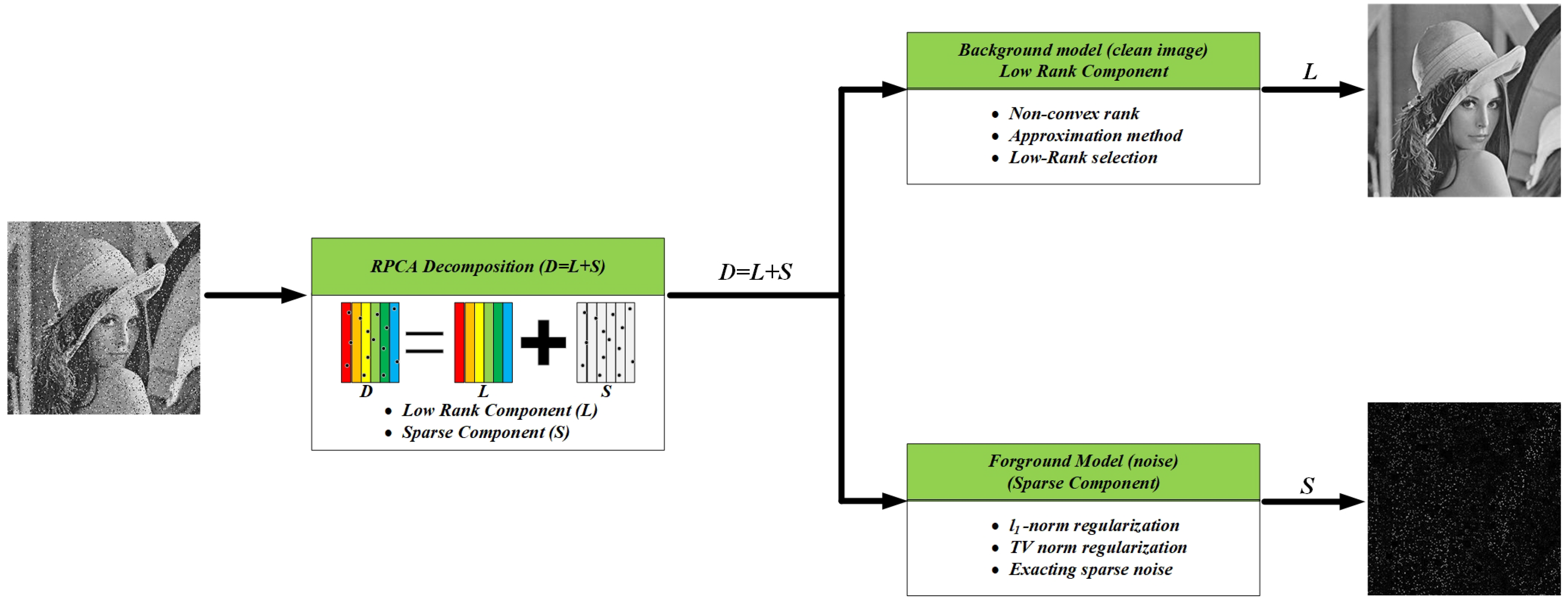
The system framework of the proposed method is presented in Figure 1. As discussed, the RPCA model based on nonconvex -norm can improve the approximation accuracy of the rank function, and the TV regularization can solve the smoothing problem of the image’s structure edge information. This section introduces our proposed RPCA model based on the nonconvex -norm and anisotropic total variation technique. The mathematical model of the method is as follows:
where D is the data matrix of the observed image; L is the low-rank matrix; S is the sparse matrix; is the -norm of the matrix L; represents the -norm of sparse matrix S; represents the TV regularization of matrix L; is a trade-off parameter for controlling the TV norm; is also a trade-off parameter; and . m and n are the dimensions of the observed image matrix D.
Figure 1.
Illustration of the proposed method.

Considering the nonconvex property of the -norm and the introduction of an anisotropic TV regularization, the augmented Lagrange multiplier algorithm [29], also known as the alternating direction method of multipliers (ADMM), is used to solve the optimization problem. We first introduce a new auxiliary variable Z into Model (6):
By adding the Lagrange multiplier and a positive punishment scalar, Formula (7) can be further derived as the following augmented Lagrange function:
where represents a penalty parameter; represents a penalty parameter; represents the inner product of two matrices, while and represent Lagrange multipliers; is the Frobenius norm of a matrix.
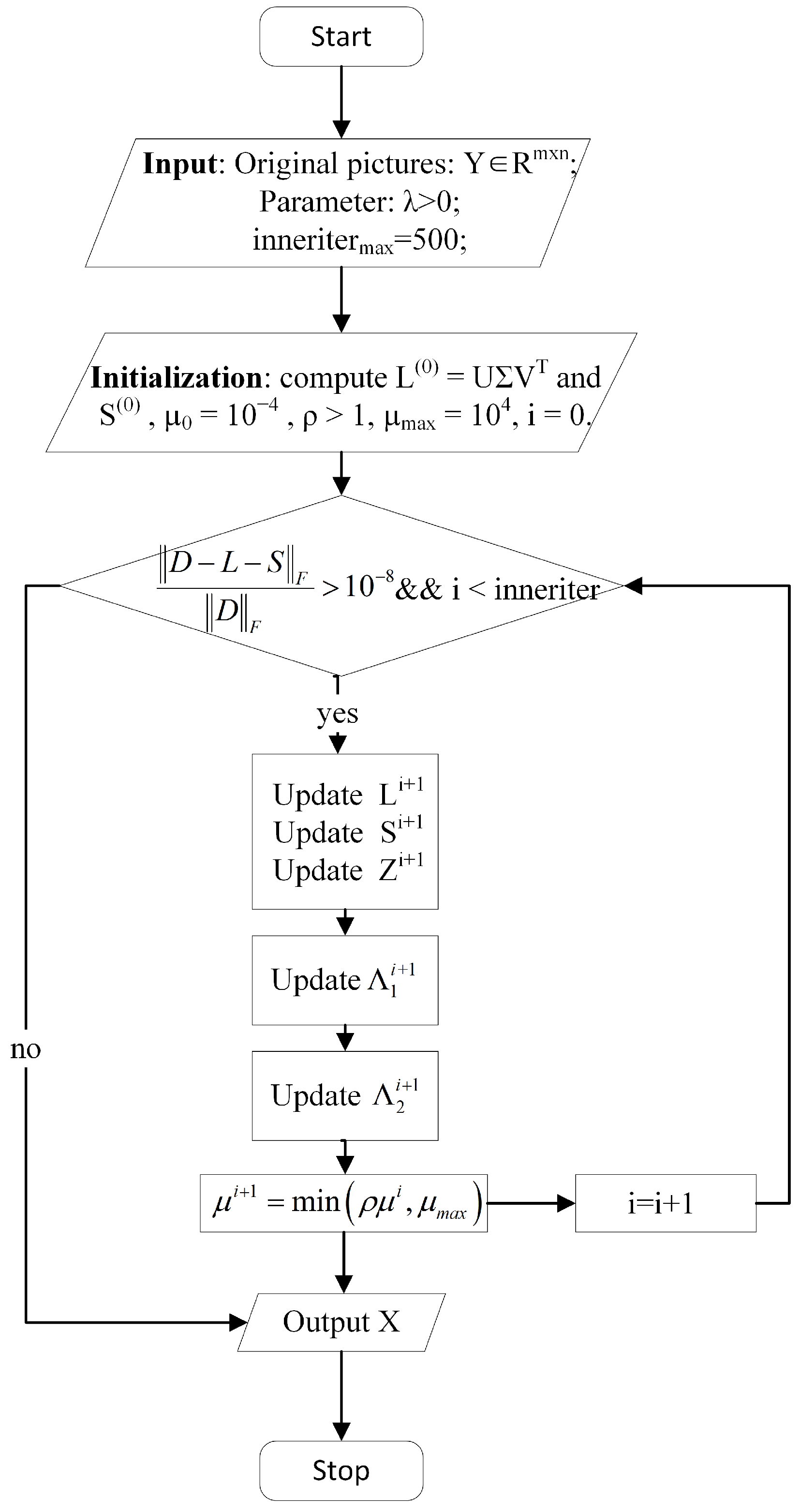
The variable L, S, Z, , and are updated under alternate iterations to improve the solution accuracy. The optimization process is summarized in Algorithm 1. The flowchart of the proposed method is presented in Figure 2.
| Algorithm 1 Solving (7) by ADMM |
Input: Observed data and Initialization: compute and , , , , While and inneriter do
Output:, . |
3.1. Updating L
To solve for variable L, we minimize over with the remaining optimization variables fixed:
To solve (9), the following theorem is introduced.
Theorem 1.
Let [42] be the SVD of and . Let be a unitarily invariant function and . Then, an optimal solution to the following problem
is , where and . Here, is the proximity operator of f with penalty μ, defined as
Based on the theorem above, the optimal solution to (9) is
where , the solution to (11), can be approximated by linearizing the concave term iteratively. Specifically, in the (k + 1) inner iteration, σ can be updated as follows:
where
![Applsci 13 07184 g002]()
Figure 2.
The flowchart of the proposed method.

and is the gradient of f at .
3.2. Updating S
The variable S is updated while minimizing over with variables fixed:
where S is the matrix of the sparse foreground part. The foreground is equivalent to an regularization. The solution is as follows:
and here, is the contraction operator which is defined as follows:
with the function returning the sign of the given operand.
3.3. Updating Z
Similarly, to solve for variable Z, we minimize over with the remaining optimization variables fixed:
We define and where optimization (18) can be rewritten as:
In this paper, we used the fast gradient-based algorithm introduced in [44] to solve (19).
3.4. Updating and
Finally, the Lagrange multiplier matrices and are updated:
4. Experimental Results and Analysis
In this section, we compare our proposed RPCA method based on a nonconvex low-rank approximation and TV regularization with five state-of-the-art methods qualitatively and quantitatively, including the robust principal component analysis (RPCA) [45], nonconvex log total variation model (AMlogtv) [46], nonconvex rank RPCA (NonRPCA) [42], weighted nuclear norm minimization–robust principal component analysis (WNNM−RPCA) [47], and total directional variation (TDV) [48]. We explore the denoising effect of our method on three common noises (salt-and-pepper noise (impulse noise), Poisson noise, and Gaussian noise). Additionally, we also perform facial image denoising experiments in Section 4.3 to demonstrate that our method is capable of preserving important image features while removing noise. An objective evaluation can avoid the uncertainty of subjective vision. Therefore, we use the peak signal-to-noise ratio (PSNR) [49], Structure similarity index measure (SSIM) [50], and feature similarity index measure (FSIM) [51] to evaluate the image quality objectively. The PSNR refers to the ratio of the maximum possible power of the maximum achievable signal strength to the destructive noise power that impacts its representation accuracy. It is often used to evaluate the quality of a denoised image compared to the original image. The SSIM is an index to measure the similarity of two images, and its value is usually affected by the brightness, contrast, and structure of the image. The FSIM is a quality assessment method based on the degree of feature similarity between the ground truth and the denoised image created using the human visual system. High values of the three metrics are desirable.
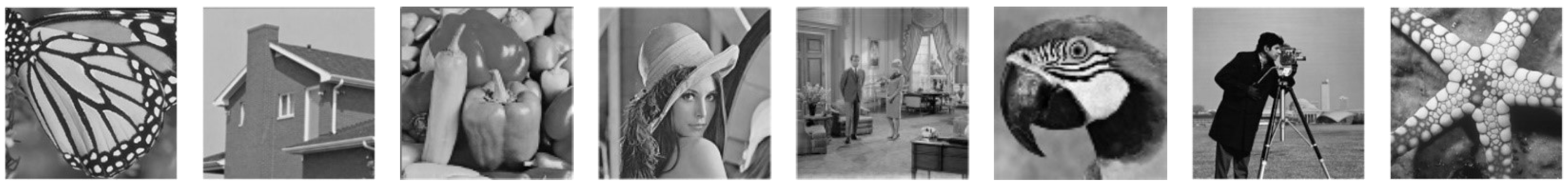
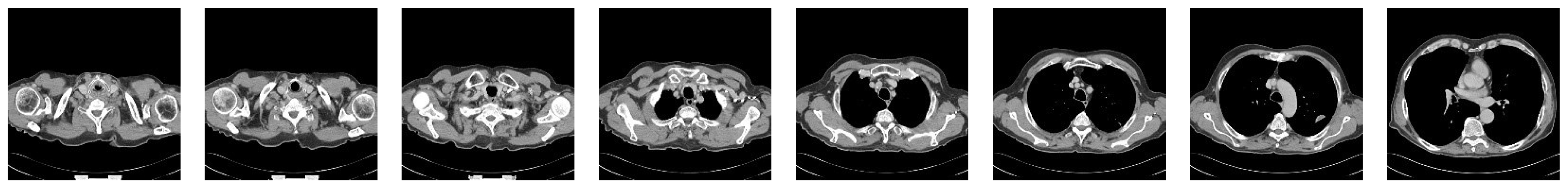
In order to verify the denoising effect of our method in different scenarios, in terms of dataset selection, we used standard, authoritative, and widely used natural image, clinical medical image, and facial image datasets for denoising experiments. The experiment used eight standard grayscale images of 256 × 256 randomly chosen from the digital image processing dataset, namely Butterfly, House, Peppers, Lena, Living Room, Bird, Camera, and Starfish. The medical image denoising experiment was conducted by randomly selecting eight 512 × 512 lung CT images from the LungCT-Diagnosis dataset (https://wiki.cancerimagingarchive.net, accessed on 26 May 2023). The data in LungCT-Diagnosis are from the Moffitt Cancer Center. The dataset has a total of 61 patients, each patient has a different number of 512 × 512 lung tumor images, and these images are diagnostic-enhanced CT scan images. In addition, the images in the Extended Yale B dataset were used in the facial image denoising experiment. The dataset has a total of 38 subjects; each subject has 64 images with a size of 192 × 168, all taken under different lighting. Due to different lighting conditions, the images of each object have different degrees of serious damage.
All the experiments in this paper were implemented in MATLAB 2018a. The host processor was an Intel(R) Core (TM) i5-9400F CPU 2.90 GHz, and the operating system was 64-bit. Furthermore, the method proposed in this paper was based on a matrix of , with the following parameter settings: , , , and .
4.1. Natural Image Denoising
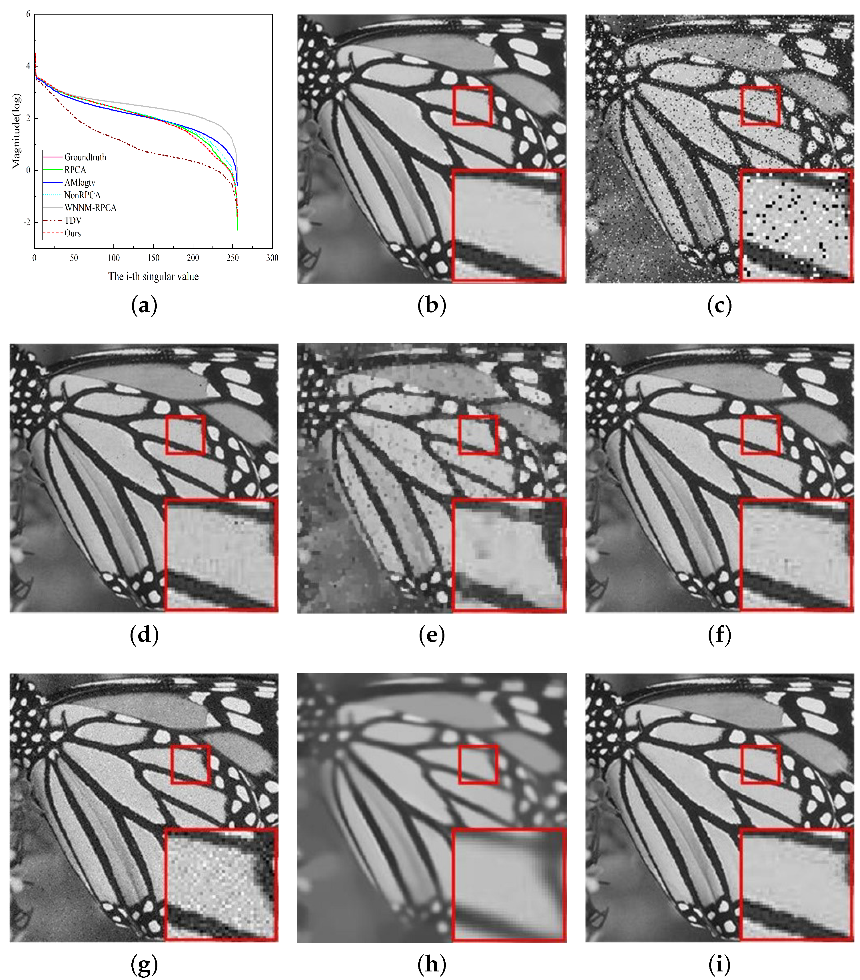
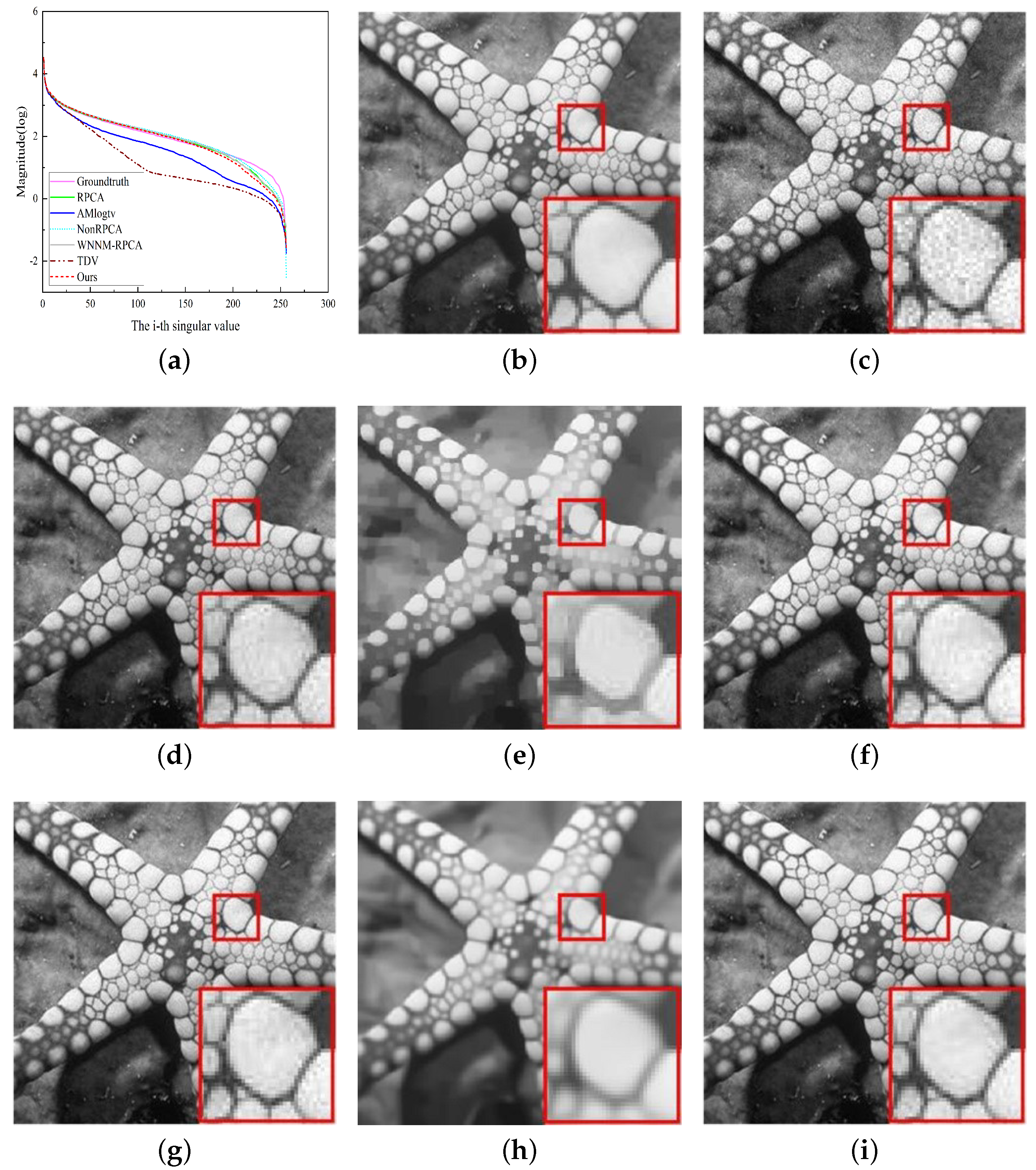
The eight natural images we selected for testing are shown in Figure 3. We chose three examples to demonstrate the denoising effect of the proposed method and five comparison methods on three types of noise, as shown in Figure 4, Figure 5 and Figure 6. In Figure 4, Figure 5 and Figure 6, example ROIs of size 30 × 30 pixels are taken (center) and enlarged (bottom right corner) for visualization, and visible image quality upgrades after restoration are presented. Additionally, based on these six methods, we compared the singular values between the original noise-free image and the denoised image, as shown in Figure 4a, Figure 5a and Figure 6a. The results showed that, compared with the five comparison methods, the singular value curve of our method was closer to the original image curve, which indicated that the method obtained the singular value closest to the original clean image.
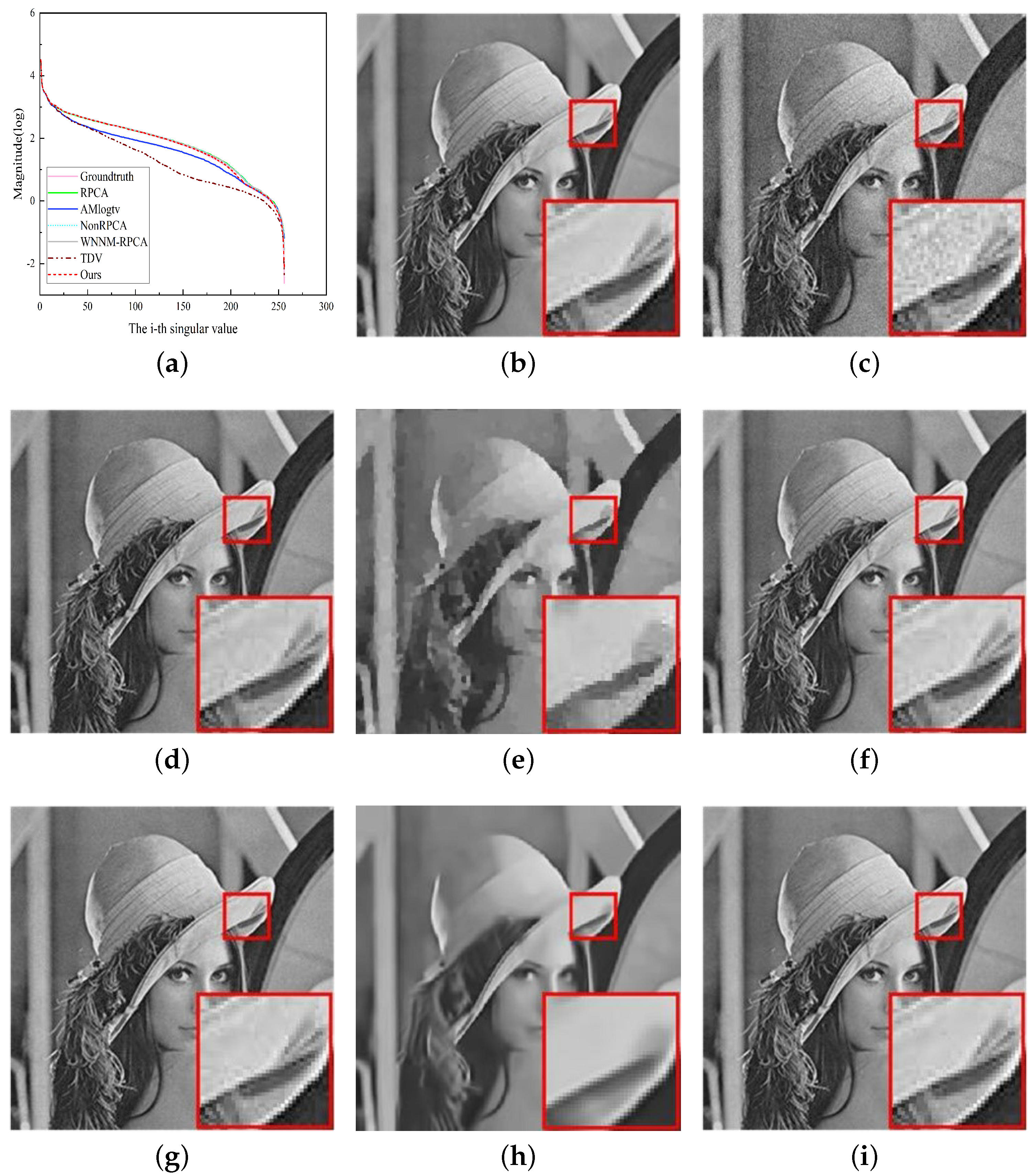
The majority of the images in Figure 4, Figure 5 and Figure 6 show that, despite the method’s various denoising impacts for different noises, our proposed method was still the best when compared to the other five methods. For example, in the denoising results of impulse noise (Figure 4), there are apparent unclear image texture phenomena in Figure 4d. Figure 4e not only retains a lot of noise, but the image structure cannot be identified either. Figure 4f has blurred edges and decreased brightness, while Figure 4g has a certain structural fidelity but a lot of noise residues. Although the noise is removed in Figure 4h, the overall appearance is very blurred, and the image edge cannot be clearly identified. Conversely, Figure 4i not only removes the noise completely but also further enhances the smoothness of the image while preserving the detailed structure of the image. This is due to the positive and effective use of our designed -norm and TV norm. In addition, our proposed method preserved the contrast and brightness of the original image well. In the Poisson noise denoising results (Figure 5), we can see that the enlarged parts of Figure 5d–g clearly show that these comparison methods blurred the noise part but did not remove the blurred part, resulting in a less clear image. The detail structure of Figure 5h is very blurred, and the overall clarity of the picture is seriously reduced. Our denoising method (Figure 5i) is more visible to the naked eye than other denoising methods and provides a smoother image. Although the overall denoising results of our method and WNNM-RPCA for Gaussian noise (Figure 6) did not differ significantly, it is nevertheless obvious from the details that our method preserved the clearest image structure and performed the most complete denoising.
Figure 5.
Denoising images of Starfish by different methods (Poisson noise). (a) Singular value comparison; (b) original clean image; (c) noisy image (Poisson noise); (d) RPCA (PSNR = 27.11 dB, SSIM = 0.9119, FSIM = 0.9561); (e) AMlogtv (PSNR = 25.65 dB, SSIM = 0.7654, FSIM = 0.9682); (f) NonRPCA (PSNR = 28.45 dB, SSIM = 0.9086, FSIM = 0.9541); (g) WNNM−RPCA (PSNR = 28.83 dB, SSIM = 0.9155, FSIM = 0.9582); (h) TDV (PSNR = 20.84 dB, SSIM = 0.5388, FSIM = 0.7005); (i) our method (PSNR = 29.30 dB, SSIM = 0.9324, FSIM = 0.9690).

We used the PSNR, SSIM, and FSIM as the objective indicators of image quality evaluation, and the data results are shown in Table 1, Table 2 and Table 3. In order to show the denoising performance of our method more intuitively, we drew histograms for the average of evaluation indexes of eight natural images under different noises according to the six methods, as shown in Figure 7. Our method achieved the best results in different noise experiments as indicated by the data from the objective indicators. In the impulse denoising experiment, our average PSNR was 23% higher than that of WNNM−RPCA, and the average SSIM was even 31% higher than that of WNNM−RPCA. In the Poisson noise denoising experiment, the average PSNR of our method was 11% higher than that of the classical algorithm RPCA, and the average FSIM was 32% higher than the TDV. In studies including Gaussian noise denoising, the average PSNR of our method was 51% better than that of AMlogtv.
Figure 6.
Denoising images of Lena by different methods (Gaussian noise). (a) Singular value comparison; (b) original clean image; (c) noisy image (Gaussian noise); (d) RPCA (PSNR = 33.61 dB, SSIM = 0.9416, FSIM = 0.9698); (e) AMlogtv (PSNR = 25.24 dB, SSIM = 0.7445, FSIM = 0.9847); (f) NonRPCA (PSNR = 37.56 dB, SSIM = 0.9437, FSIM = 0.9712); (g) WNNM−RPCA (PSNR = 38.86 dB, SSIM = 0.9539, FSIM = 0.9766); (h) TDV (PSNR = 23.03 dB, SSIM = 0.6737, FSIM = 0.7617); (i) our method (PSNR = 42.37 dB, SSIM = 0.9795, FSIM = 0.9890).

4.2. Medical Image Denoising
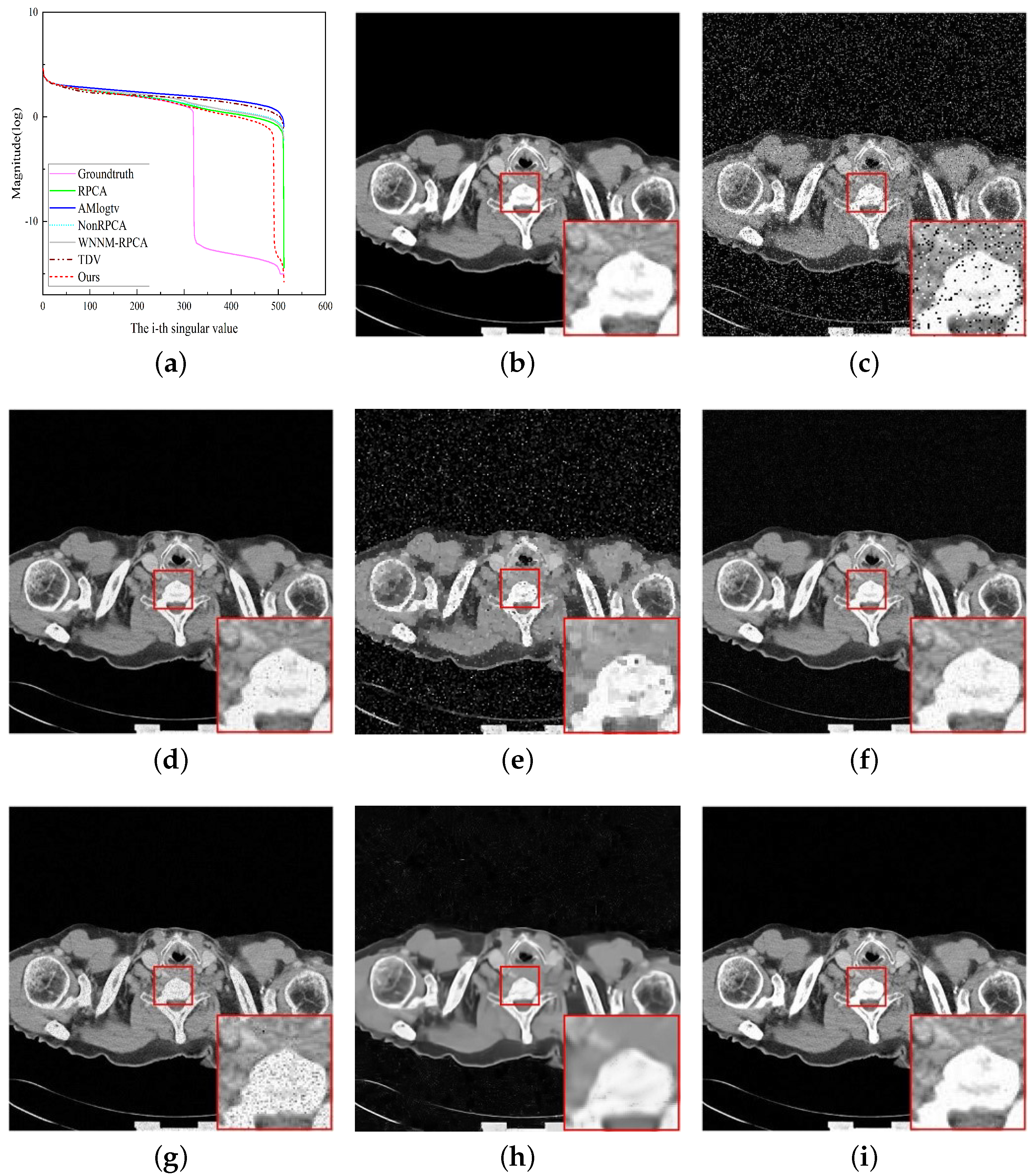
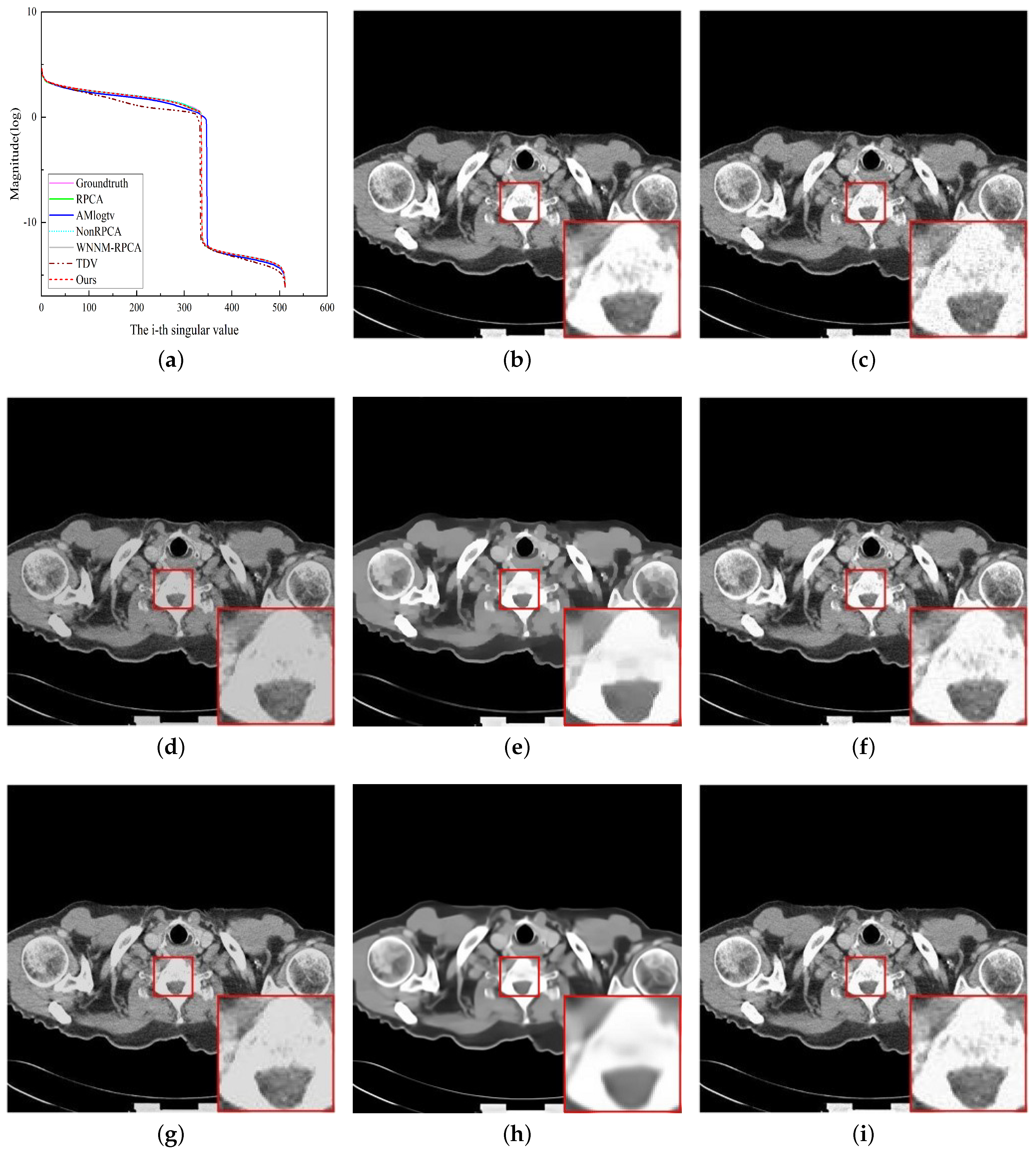
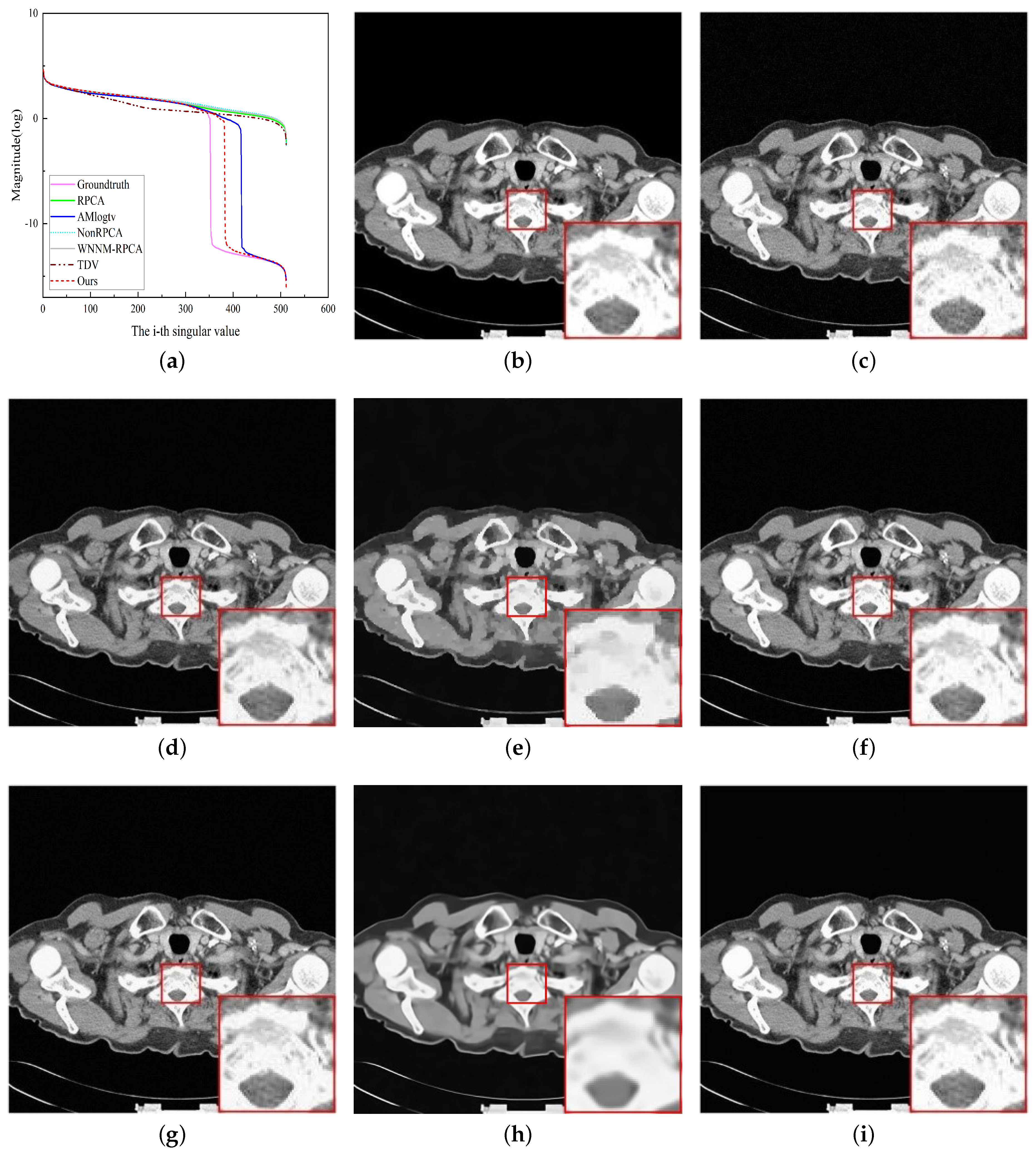
In this section, we selected eight medical images from public datasets for testing, as shown in Figure 8. We show the visual comparison results of three images in Figure 9, Figure 10 and Figure 11. Among them, Figure 9a, Figure 10a, and Figure 11a are the singular value distribution curves of the denoised image and the original image of each comparison method. We learn that the singular value of the denoised image obtained by the proposed method is closer to the real ground value, which also proves that it has the advantage of suppressing the overpenalized singular value of the classical competition method (RPCA) while maintaining a small singular value.
By observing the denoising experiment findings, we discover that in the denoising results of impulse noise (Figure 9), the enlarged images of Figure 9d,h have clear artifacts and little to no noise. In the enlarged image of Figure 9e, the noise is mixed with the structure of the image itself, and the image and noise cannot be distinguished. Although there is not any evident noise in the magnified version of Figure 9f, there is a small blurring of the edge information of the lung tissue and some “oil painting” phenomenon. In Figure 9g, there is a great deal of noise, which makes the image unrecognizable. The enlarged image of Figure 9h is very blurred, and there is obvious noise in the image. Conversely, our method (Figure 9i) has the best denoising effect. The image edge structure is highly clear and noise-free, which is nearly identical to the original image. In the experiment of removing Poisson noise, we find that although the denoising effects of these six algorithms are very close, we can still find that Figure 10d,g are obviously darkened, and there are still some impurities in the background of Figure 10f. Figure 10e,h blur the original details of the image, but our method (Figure 10i) does not exhibit these phenomena. Furthermore, when denoising the image containing Gaussian noise, it is obvious from the comparison result diagram in Figure 11 that although the comparison method removes noise to a certain extent, it does not smooth the image when saving the image detail information, leaving the image with insufficient clarity. In conclusion, our approach had a good edge recovery effect, entirely preserved lung parenchyma, and effectively reduced noise. It can be determined that our denoising method was superior to other methods by a subjective visual evaluation.
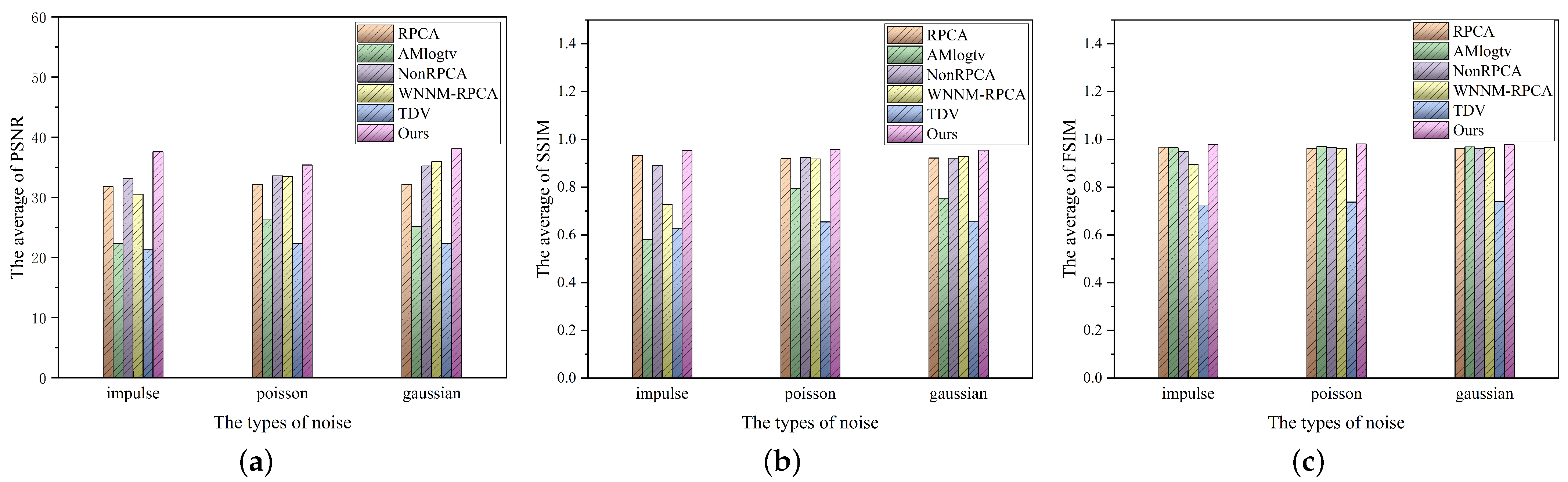
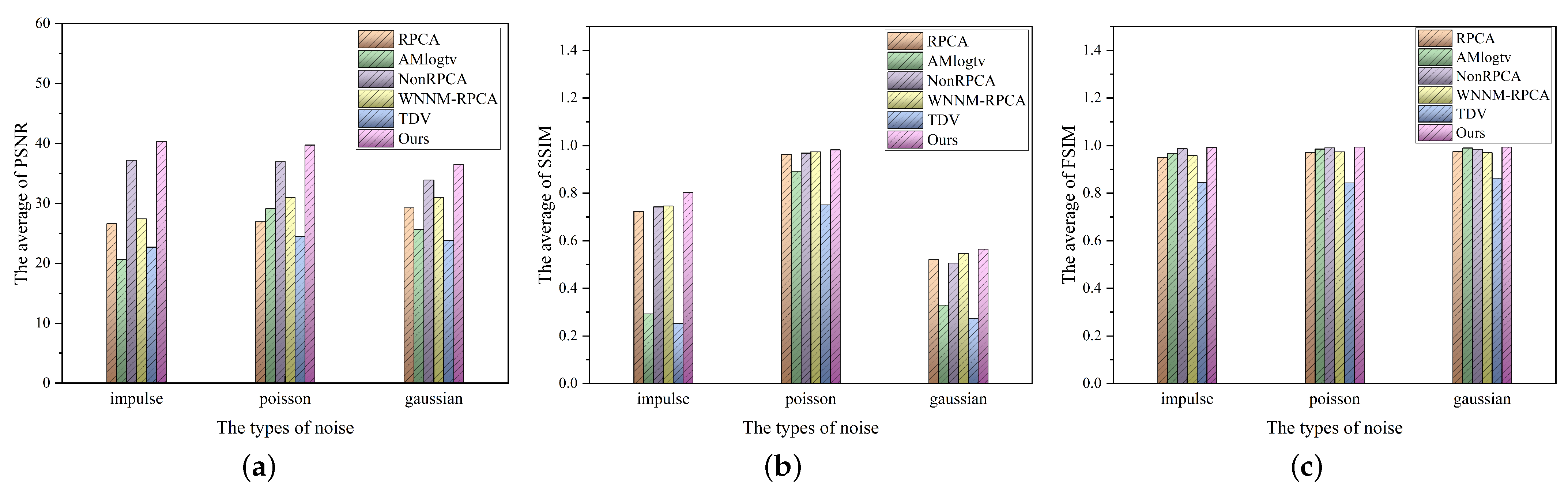
The objective evaluation is shown in Table 4, Table 5 and Table 6 and Figure 12. It can be seen from Figure 12 that our proposed method also achieved the best effect in medical image denoising. Specifically, when denoising impulse noise, the average PSNR value of NonRPCA was roughly 40% higher than that of the classical RPCA algorithm, and the average PSNR value of our method was about 8% higher than that of NonRPCA. For Poisson noise, the average PSNR of our method was 36% higher than the latest method, AMlogtv, and the average SSIM was 31% higher than TDV, which also showed the effectiveness of our method. Additionally, against the background of Gaussian noise, the average SSIM values of all methods were low, which may be due to the characteristics of Gaussian noise itself, causing the brightness, contrast, and image structure to affect the SSIM value. Moreover, the average SSIM value of our proposed method was still higher than other methods. In summary, the objective evaluation results of images were essentially consistent with the subjective analysis.
Figure 8.
The LungCT images used in our experiments. The image numbers are given from left to right as 1 to 8.
Figure 8.
The LungCT images used in our experiments. The image numbers are given from left to right as 1 to 8.

Figure 9.
Denoising images of LungCT image no. 1 by different methods (impulse noise). (a) Singular value comparison; (b) original clean image; (c) noisy image (impulse noise); (d) RPCA (PSNR = 34.11 dB, SSIM = 0.8401, FSIM = 0.9904); (e) AMlogtv (PSNR = 20.81 dB, SSIM = 0.2979, FSIM = 0.9630); (f) NonRPCA (PSNR = 39.39 dB, SSIM = 0.7965, FSIM = 0.9924); (g) WNNM−RPCA (PSNR = 30.07 dB, SSIM = 0.7915, FSIM = 0.9761); (h) TDV (PSNR = 22.66 dB, SSIM = 0.2491, FSIM = 0.8230); (i) our method (PSNR = 43.94 dB, SSIM = 0.8709, FSIM = 0.9968).

Figure 10.
Denoising images of LungCT image no. 2 by different methods (Poisson noise). (a) Singular value comparison; (b) original clean image; (c) noisy image (Poisson noise); (d) RPCA (PSNR = 25.99 dB, SSIM = 0.9620, FSIM = 0.9656); (e) AMlogtv (PSNR = 29.25 dB, SSIM = 0.8792, FSIM = 0.9870); (f) NonRPCA (PSNR = 37.75 dB, SSIM = 0.9732, FSIM = 0.9918); (g) WNNM−RPCA (PSNR = 31.22 dB, SSIM = 0.9776, FSIM = 0.9786); (h) TDV (PSNR = 23.51 dB, SSIM = 0.6897, FSIM = 0.8187); (i) our method (PSNR = 41.38 dB, SSIM = 0.9895, FSIM = 0.9956).

Figure 11.
Denoising images of LungCT image no. 3 by different methods (Gaussian noise). (a) Singular value comparison; (b) original clean image; (c) noisy image (Gaussian noise); (d) RPCA (PSNR = 33.85 dB, SSIM = 0.6098, FSIM = 0.9916); (e) AMlogtv (PSNR = 25.68 dB, SSIM = 0.3639, FSIM = 0.9968); (f) NonRPCA (PSNR = 34.89 dB, SSIM = 0.5844, FSIM = 0.9867); (g) WNNM−RPCA (PSNR = 35.28 dB, SSIM = 0.5988, FSIM = 0.9890); (h) TDV (PSNR = 23.30 dB, SSIM = 0.2879, FSIM = 0.8248); (i) our method (PSNR = 37.94 dB, SSIM = 0.6233, FSIM = 0.9980).

Figure 12.
Histogram of evaluation indicators of medical images. (a) Average PSNR; (b) average SSIM; (c) average FSIM.
Figure 12.
Histogram of evaluation indicators of medical images. (a) Average PSNR; (b) average SSIM; (c) average FSIM.


Table 4.
PSNR comparisons of RPCA, AMlogtv, NonRPCA, WNNM−RPCA, TDV, and the proposed method for noise removal in LungCT images (optimal value: red line; suboptimal value: cyan line).
Table 4.
PSNR comparisons of RPCA, AMlogtv, NonRPCA, WNNM−RPCA, TDV, and the proposed method for noise removal in LungCT images (optimal value: red line; suboptimal value: cyan line).
| Noise Type | Images | RPCA | AMlogtv | NonRPCA | WNNM−RPCA | TDV | Ours |
|---|---|---|---|---|---|---|---|
| Impulse noise | 1 | 34.1086 | 20.8109 | 39.3910 | 30.0661 | 22.6606 | 43.9398 |
| 2 | 29.7339 | 20.7488 | 39.8981 | 28.6808 | 22.5140 | 42.6776 | |
| 3 | 27.5287 | 20.7872 | 36.5463 | 29.3167 | 22.3062 | 40.9121 | |
| 4 | 34.5260 | 20.7857 | 41.9476 | 31.1892 | 22.3296 | 43.9249 | |
| 5 | 22.7421 | 20.6817 | 36.5971 | 26.6155 | 22.6972 | 39.0744 | |
| 6 | 21.6578 | 20.5327 | 36.2646 | 24.5502 | 23.0144 | 38.7777 | |
| 7 | 21.5732 | 20.4626 | 33.8149 | 25.8391 | 23.0563 | 36.7197 | |
| 8 | 20.8001 | 20.3707 | 32.7776 | 22.9537 | 22.9246 | 36.3267 | |
| Average | 26.5838 | 20.6475 | 37.1546 | 27.4014 | 22.6878 | 40.2941 | |
| Poisson noise | 1 | 25.3796 | 29.2750 | 37.8533 | 30.4089 | 23.4745 | 40.7487 |
| 2 | 25.9954 | 29.2576 | 37.7551 | 31.2219 | 23.5091 | 41.3824 | |
| 3 | 32.0855 | 29.0463 | 40.0718 | 40.0718 | 23.8365 | 42.0702 | |
| 4 | 27.2295 | 29.0262 | 39.0888 | 32.7282 | 24.2402 | 40.3903 | |
| 5 | 24.7137 | 29.2884 | 35.0703 | 27.0225 | 23.7425 | 38.5899 | |
| 6 | 25.3914 | 29.0887 | 36.5243 | 27.4036 | 22.3025 | 40.6466 | |
| 7 | 28.2686 | 28.8807 | 29.3977 | 31.1992 | 27.3887 | 37.9662 | |
| 8 | 26.2732 | 28.8691 | 33.4158 | 28.9564 | 27.4388 | 35.8507 | |
| Average | 26.9171 | 29.0915 | 36.9186 | 30.9760 | 24.4916 | 39.7056 | |
| Gaussian noise | 1 | 29.0228 | 25.7441 | 34.9713 | 32.3936 | 23.5661 | 37.0809 |
| 2 | 29.0297 | 25.7769 | 33.8007 | 33.1549 | 23.5022 | 37.4827 | |
| 3 | 33.8497 | 25.6839 | 34.8873 | 35.2871 | 23.2967 | 37.9355 | |
| 4 | 30.3547 | 25.6564 | 33.3377 | 31.6763 | 23.4633 | 35.8458 | |
| 5 | 27.5425 | 25.7290 | 34.7948 | 30.7608 | 23.7899 | 36.1815 | |
| 6 | 27.9469 | 25.5031 | 32.8209 | 28.5334 | 24.3505 | 35.7714 | |
| 7 | 26.7573 | 25.4181 | 32.1886 | 27.2011 | 24.4782 | 34.9603 | |
| 8 | 29.3714 | 25.3123 | 34.1811 | 28.4058 | 24.1735 | 36.1523 | |
| Average | 29.2344 | 25.6030 | 33.8728 | 30.9266 | 23.8275 | 36.4263 |
The Average values are in bold black.
Table 5.
SSIM comparisons of RPCA, AMlogtv, NonRPCA, WNNM−RPCA, TDV, and the proposed method for noise removal in LungCT images (optimal value: red line; suboptimal value: cyan line).
Table 5.
SSIM comparisons of RPCA, AMlogtv, NonRPCA, WNNM−RPCA, TDV, and the proposed method for noise removal in LungCT images (optimal value: red line; suboptimal value: cyan line).
| Noise Type | Images | RPCA | AMlogtv | NonRPCA | WNNM−RPCA | TDV | Ours |
|---|---|---|---|---|---|---|---|
| Impulse noise | 1 | 0.8401 | 0.2979 | 0.7965 | 0.7915 | 0.2491 | 0.8709 |
| 2 | 0.7893 | 0.3024 | 0.7830 | 0.7847 | 0.2533 | 0.8524 | |
| 3 | 0.7605 | 0.3158 | 0.7402 | 0.7937 | 0.2670 | 0.8437 | |
| 4 | 0.8474 | 0.3109 | 0.8179 | 0.7987 | 0.2618 | 0.8750 | |
| 5 | 0.6546 | 0.2922 | 0.7103 | 0.7359 | 0.2513 | 0.7766 | |
| 6 | 0.6337 | 0.2741 | 0.6918 | 0.7015 | 0.2475 | 0.7741 | |
| 7 | 0.6276 | 0.2690 | 0.7090 | 0.7140 | 0.2481 | 0.7159 | |
| 8 | 0.6285 | 0.2732 | 0.6860 | 0.6430 | 0.2437 | 0.7080 | |
| Average | 0.7227 | 0.2919 | 0.7418 | 0.7453 | 0.2527 | 0.8020 | |
| Poisson noise | 1 | 0.9589 | 0.8826 | 0.9740 | 0.9766 | 0.6923 | 0.9883 |
| 2 | 0.9620 | 0.8792 | 0.9732 | 0.9776 | 0.6897 | 0.9895 | |
| 3 | 0.9816 | 0.8739 | 0.9847 | 0.9840 | 0.7149 | 0.9903 | |
| 4 | 0.9654 | 0.8779 | 0.9794 | 0.9774 | 0.7430 | 0.9840 | |
| 5 | 0.9479 | 0.8940 | 0.9539 | 0.9610 | 0.7055 | 0.9791 | |
| 6 | 0.9573 | 0.9022 | 0.9628 | 0.9664 | 0.6900 | 0.9821 | |
| 7 | 0.9682 | 0.9070 | 0.9658 | 0.9734 | 0.8766 | 0.9745 | |
| 8 | 0.9600 | 0.9160 | 0.9509 | 0.9645 | 0.8944 | 0.9694 | |
| Average | 0.9626 | 0.8916 | 0.9680 | 0.9726 | 0.7508 | 0.9821 | |
| Gaussian noise | 1 | 0.5095 | 0.3330 | 0.5307 | 0.5627 | 0.2681 | 0.5862 |
| 2 | 0.5185 | 0.3425 | 0.5144 | 0.5737 | 0.2739 | 0.5981 | |
| 3 | 0.6098 | 0.3639 | 0.5844 | 0.5988 | 0.2879 | 0.6233 | |
| 4 | 0.5725 | 0.3535 | 0.5310 | 0.5790 | 0.2866 | 0.5832 | |
| 5 | 0.5293 | 0.3287 | 0.5352 | 0.5428 | 0.2726 | 0.5680 | |
| 6 | 0.4550 | 0.3071 | 0.4537 | 0.5142 | 0.2696 | 0.5432 | |
| 7 | 0.4861 | 0.3042 | 0.4412 | 0.5022 | 0.2716 | 0.5115 | |
| 8 | 0.4883 | 0.2991 | 0.4628 | 0.5005 | 0.2657 | 0.5224 | |
| Average | 0.5211 | 0.3290 | 0.5067 | 0.5467 | 0.2745 | 0.5669 |
The Average values are in bold black.
Table 6.
FSIM comparisons of RPCA, AMlogtv, NonRPCA, WNNM−RPCA, TDV, and the proposed method for noise removal in LungCT images (optimal value: red line; suboptimal value: cyan line).
Table 6.
FSIM comparisons of RPCA, AMlogtv, NonRPCA, WNNM−RPCA, TDV, and the proposed method for noise removal in LungCT images (optimal value: red line; suboptimal value: cyan line).
| Noise Type | Images | RPCA | AMlogtv | NonRPCA | WNNM−RPCA | TDV | Ours |
|---|---|---|---|---|---|---|---|
| Impulse noise | 1 | 0.9904 | 0.9630 | 0.9924 | 0.9761 | 0.8230 | 0.9968 |
| 2 | 0.9761 | 0.9656 | 0.9928 | 0.9675 | 0.8219 | 0.9956 | |
| 3 | 0.9645 | 0.9709 | 0.9880 | 0.9662 | 0.8086 | 0.9938 | |
| 4 | 0.9907 | 0.9657 | 0.9952 | 0.9759 | 0.8328 | 0.9759 | |
| 5 | 0.9392 | 0.9652 | 0.9850 | 0.9602 | 0.8573 | 0.9912 | |
| 6 | 0.9243 | 0.9651 | 0.9827 | 0.9441 | 0.8681 | 0.9909 | |
| 7 | 0.9159 | 0.9665 | 0.9816 | 0.9501 | 0.8771 | 0.9870 | |
| 8 | 0.9057 | 0.9732 | 0.9831 | 0.9226 | 0.8658 | 0.9879 | |
| Average | 0.9508 | 0.9669 | 0.9876 | 0.9578 | 0.8443 | 0.9925 | |
| Poisson noise | 1 | 0.9619 | 0.9900 | 0.9919 | 0.9769 | 0.8163 | 0.9954 |
| 2 | 0.9656 | 0.9870 | 0.9918 | 0.9786 | 0.8187 | 0.9956 | |
| 3 | 0.9917 | 0.9775 | 0.9938 | 0.9928 | 0.8221 | 0.9957 | |
| 4 | 0.9756 | 0.9673 | 0.9939 | 0.9834 | 0.8533 | 0.9945 | |
| 5 | 0.9490 | 0.9921 | 0.9899 | 0.9504 | 0.8443 | 0.9944 | |
| 6 | 0.9570 | 0.9880 | 0.9905 | 0.9577 | 0.7483 | 0.9943 | |
| 7 | 0.9846 | 0.9902 | 0.9898 | 0.9771 | 0.9213 | 0.9917 | |
| 8 | 0.9782 | 0.9885 | 0.9844 | 0.9687 | 0.9231 | 0.9894 | |
| Average | 0.9704 | 0.9851 | 0.9907 | 0.9732 | 0.8434 | 0.9938 | |
| Gaussian noise | 1 | 0.9749 | 0.9944 | 0.9907 | 0.9907 | 0.8388 | 0.9949 |
| 2 | 0.9752 | 0.9961 | 0.9882 | 0.9821 | 0.8374 | 0.9965 | |
| 3 | 0.9916 | 0.9968 | 0.9867 | 0.9890 | 0.8248 | 0.9980 | |
| 4 | 0.9821 | 0.9770 | 0.9823 | 0.9760 | 0.8547 | 0.9960 | |
| 5 | 0.9640 | 0.9902 | 0.9840 | 0.9701 | 0.8755 | 0.9909 | |
| 6 | 0.9698 | 0.9873 | 0.9782 | 0.9601 | 0.8884 | 0.9890 | |
| 7 | 0.9603 | 0.9848 | 0.9756 | 0.9478 | 0.8935 | 0.9853 | |
| 8 | 0.9791 | 0.9915 | 0.9893 | 0.9625 | 0.8858 | 0.9926 | |
| Average | 0.9746 | 0.9897 | 0.9844 | 0.9709 | 0.8623 | 0.9929 |
The Average values are in bold black.
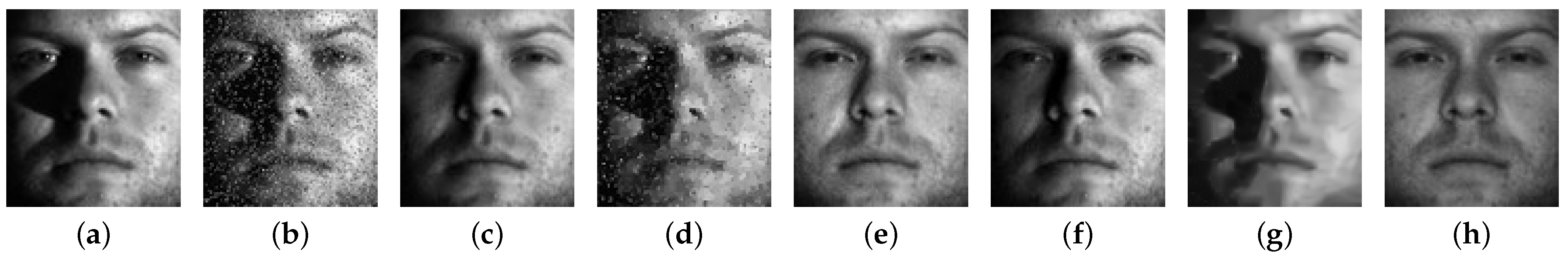
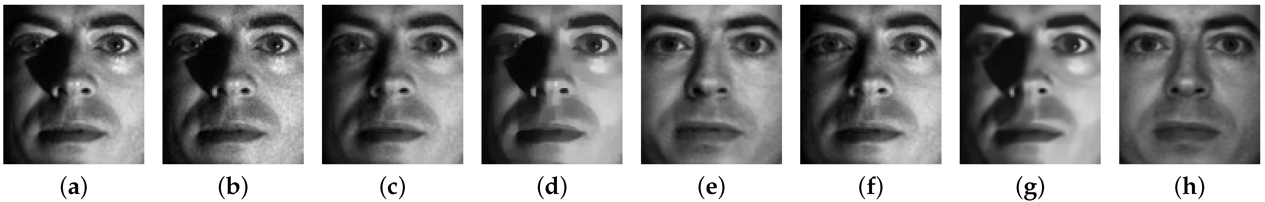
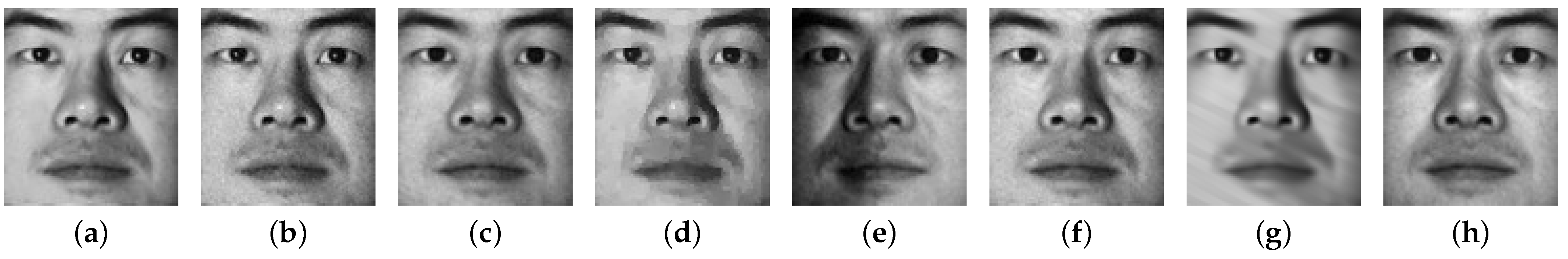
4.3. Face Denoising with Illumination Variation
Face images of the same subject under different illumination conditions generally lie in a low-dimensional subspace, while the outliers resulting from lighting variations can be assumed to be sparse [52]. RPCA can therefore balance the uneven brightness of the image surface and retain important facial features while removing noise. Moreover, given enough facial images of the same person, it is possible to reconstruct real facial images. We experimented with 64 images from the Extended Yale B database for each participant. All images were converted to 32,256-dimensional column vectors, hence for each subject. Since the images were well aligned, L should have a rank of one.
In order to demonstrate the effectiveness of the proposed method, we selected facial images of three subjects from the Extended Yale B database and added different noises to each subject to demonstrate the method’s performance, as shown in Figure 13, Figure 14 and Figure 15. By observing these three sets of photos, it can be shown that in comparison to the experimental outcomes of the comparison methods, the proposed method could more effectively remove the occlusion shadow of the image and keep the important features of the face image on the basis of successfully removing the noise, thereby restoring the true face image. The denoising results of RPCA and WNNM-RPCA were similar, and all of them eliminated a significant amount of noise when removing impulse noise (Figure 13). However, the brightness of the image surface was unbalanced, making it difficult to clearly distinguish facial characteristics. The AMlogtv method could not remove noise in facial images. The TDV method removed noise, but the shadow in the image was not removed, which made the face difficult to identify. Although NonRPCA removed most of the shadows of the face, the denoised image was not smooth enough to cause the detail structure to be very blurred. Similarly, even when removing Poisson and Gaussian noise, respectively, these comparison methods’ denoising effects remained poor. For instance, when removing Poisson noise (Figure 14), WNNM-RPCA (Figure 14f) had the worst impact, not only not entirely removing the noise but also leaving half of the facial image in the shadow. Although NonRPCA (Figure 14e) preserved facial features well, it produced some artifacts in the denoising process. When removing Gaussian noise (Figure 15), RPCA (Figure 15c) and AMlogtv (Figure 15d) still had a small amount of noise, and the uneven brightness of the image surface was not balanced, which blocked the facial features of the image. It can be seen that the experimental effect of our method was the best.
4.4. Implementation Computational Cost
To verify the time cost performance of the proposed method, the starfish image with impulse noise and a size of 256 × 256 was chosen as the test image.
As shown in Table 7, the running time of the proposed method was shorter compared with that of NonRPCA and TDV. Although the running time of the proposed method was longer compared with that of RPCA, AMlogtv, and WNNM-RPCA, the denoising effect of the proposed method was significantly higher than that of the above three methods. The proposed method sacrificed a certain degree of computational cost and improved the accuracy of image restoration.
Figure 13.
Denoising images of yaleB01 by different methods (impulse noise). (a) Original facial image; (b) noisy image (impulse noise); (c) RPCA; (d) AMlogtv; (e) NonRPCA; (f) WNNM-RPCA; (g) TDV; (h) our method.
Figure 13.
Denoising images of yaleB01 by different methods (impulse noise). (a) Original facial image; (b) noisy image (impulse noise); (c) RPCA; (d) AMlogtv; (e) NonRPCA; (f) WNNM-RPCA; (g) TDV; (h) our method.

Figure 14.
Denoising images of yaleB06 by different methods (Poisson noise). (a) Original facial image; (b) noisy image (Poisson noise); (c) RPCA; (d) AMlogtv; (e) NonRPCA; (f) WNNM-RPCA; (g) TDV; (h) our method.
Figure 14.
Denoising images of yaleB06 by different methods (Poisson noise). (a) Original facial image; (b) noisy image (Poisson noise); (c) RPCA; (d) AMlogtv; (e) NonRPCA; (f) WNNM-RPCA; (g) TDV; (h) our method.

Figure 15.
Denoising images of yaleB02 by different methods (Gaussian noise). (a) Original facial image; (b) noisy image (Gaussian noise); (c) RPCA; (d) AMlogtv; (e) NonRPCA; (f) WNNM-RPCA; (g) TDV; (h) our method.
Figure 15.
Denoising images of yaleB02 by different methods (Gaussian noise). (a) Original facial image; (b) noisy image (Gaussian noise); (c) RPCA; (d) AMlogtv; (e) NonRPCA; (f) WNNM-RPCA; (g) TDV; (h) our method.

5. Conclusions
In this study, we proposed a low-rank matrix approximation method that combined the nonconvex -norm, the -norm, and the anisotropic TV regularization to remove noise in images. A denoising experiment on standard natural images, clinical medical images, and facial images was carried out in this paper. The results showed that: (1) When compared with five state-of-the-art methods (RPCA, AMlogtv, NonRPCA, WNNM-RPCA, and TDV), our method was superior in terms of clarity, brightness, and detail characterization, and its denoising results were more consistent with subjective vision. (2) In the objective analysis, the quantitative results based on PSNR, SSIM, and FSIM showed that our method had higher scores, and the objective index was obviously improved compared with some methods. In addition, in the experiment of removing facial image noise, our method could highlight facial features more clearly, without artifacts, while removing noise. At the same time, our method had a lower computational cost than NonRPCA and TDV. Although its cost was higher than the other three methods, our denoising effect was better than theirs. To summarize, the proposed RPCA framework based on a nonconvex low-rank approximation and TV norm showed good performance in noise removal and in the retention of important features of images, which provides a reference for the future application of nonconvex functions in the field of image denoising. However, our method can only process grayscale images at present, and it needs to be optimized in terms of computational cost. Therefore, in the future, we will continue to investigate new iterative optimization methods for solving nonconvex optimization problems, as well as extend our research to a tensor framework for solving the problem of color image denoising in complex noise backgrounds.
Author Contributions
Conceptualization, T.C., Q.X. and D.Z.; methodology, T.C., Q.X. and D.Z.; formal analysis, Q.X.; resources, T.C., Q.X., D.Z. and L.S.; data curation, T.C. and Q.X.; writing—original draft preparation, T.C., Q.X. and D.Z.; writing—review and editing, T.C. and Q.X. All authors have read and agreed to the published version of the manuscript.
Funding
This work was supported by the National Natural Science Foundation of China under grant nos. 62173127 and 61973104, the Scientific and Technological Innovation Leaders in Central Plains (no. 224200510008), the Henan Excellent Young Scientists Fund (no. 212300410036), the Program for Science and Technology Innovation Talents in Universities of Henan Province under grant no. 21HASTIT029, the Innovative Funds Plans of Henan University of Technology under grant no. 2020ZKCJ06, the Zhengzhou Science and Technology Collaborative Innovation Project (no. 21ZZXTCX06), the Cultivation Program of Young Backbone Teachers in Henan University of Technology under grant chentianfei, the Open Fund from Research Platform of Grain Information Processing Center in Henan University of Technology under grant no. KFJJ-2022-003.
Institutional Review Board Statement
Not applicable.
Informed Consent Statement
Not applicable.
Data Availability Statement
The data used to support this study are available from the corresponding author upon request.
Conflicts of Interest
The authors declare no conflict of interest.
Abbreviations
| RPCA | Robust principal component analysis |
| TV | Total variational regularization |
| AWRR | Adaptive weighted rank reduction |
| SJSCCA | Structured joint sparse canonical correlation analysis |
| SR | Sparse representation |
| LMMSE | Linear minimum mean-squared error estimator |
| CT | Computed tomography |
| PSNR | Peak signal-to-noise ratio |
| SSIM | Structure similarity index measure |
| FSIM | Feature similarity index measure |
References
- Diwakar, M.; Singh, P. CT image denoising using multivariate model and its method noise thresholding in non-subsampled shearlet domain. Biomed. Signal Process. Control 2021, 57, 101754. [Google Scholar] [CrossRef]
- Fan, L.; Zhang, F.; Fan, H.; Zhang, C. Brief review of image denoising techniques. Vis. Comput. Ind. Biomed. Art 2019, 2, 7. [Google Scholar] [CrossRef] [PubMed]
- Pradeep, S.; Nirmaladevi, P. A review on speckle noise reduction techniques in ultrasound medical images based on spatial domain, transform domain and CNN methods. In IOP Conference Series: Materials Science and Engineering; IOP Conference: Erode, India, 2021; p. 012116. [Google Scholar]
- Rakshit, S.; Ghosh, A.; Shankar, B.U. Fast mean filtering technique (FMFT). Pattern Recognit. 2007, 40, 890–897. [Google Scholar] [CrossRef]
- Justusson, B.I. Median filtering: Statistical properties. In Two-Dimensional Digital Signal Prcessing II: Transforms and Median Filters; Springer: Berlin/Heidelberg, Germany, 2006; pp. 161–196. [Google Scholar]
- Chen, J.; Benesty, J.; Huang, Y.; Doclo, S. New insights into the noise reduction Wiener filter. IEEE Trans. Audio Speech Lang. Process. 2006, 14, 1218–1234. [Google Scholar] [CrossRef]
- Özen Acarbay, E.; Özkurt, N. Performance analysis of the speech enhancement application with wavelet transform domain adaptive filters. Int. J. Speech Technol. 2023, 26, 245–258. [Google Scholar] [CrossRef]
- Grotevent, M.J.; Yakunin, S.; Bachmann, D.; Romero, C.; Vázquez de Aldana, J.R.; Madi, M.; Calame, M.; Kovalenko, M.V.; Shorubalko, I. Integrated photodetectors for compact Fourier-transform waveguide spectrometers. Nat. Photon. 2023, 17, 59–64. [Google Scholar] [CrossRef]
- Scribano, C.; Franchini, G.; Prato, M.; Bertogna, M. DCT-Former: Efficient Self-Attention with Discrete Cosine Transform. J. Sci. Comput. 2023, 94, 67. [Google Scholar] [CrossRef]
- Scribano, C.; Zheng, M.; Prato, M.; Zuo, W.; Zhang, B.; Zhang, Y.; Zhang, D. Multi-stage image denoising with the wavelet transform. Pattern Recognit. 2023, 134, 109050. [Google Scholar]
- Farmani, B.; Pal, Y.; Pedersen, M. Motion sensor noise attenuation using deep learning. First Break 2023, 41, 45–51. [Google Scholar] [CrossRef]
- Wang, S.; Nie, F.; Wang, Z.; Wang, R.; Li, X. Robust Principal Component Analysis via Joint Reconstruction and Projection. IEEE Trans. Neural Netw. Learn. Syst. 2022. early access. [Google Scholar] [CrossRef]
- Pokala, P.K.; Hemadri, R.V.; Seelamantula, C.S. Iteratively reweighted minimax-concave penalty minimization for accurate low-rank plus sparse matrix decomposition. IEEE Trans. Pattern Anal. Mach. Intell. 2021, 44, 8992–9010. [Google Scholar] [CrossRef]
- Bayati, F.; Trad, D. 3-D Data Interpolation and Denoising by an Adaptive Weighting Rank-Reduction Method Using Multichannel Singular Spectrum Analysis Algorithm. Sensors 2023, 23, 577. [Google Scholar] [CrossRef]
- Wang, L.; Xiao, D.; Hou, W.S. Weighted Schatten p-norm minimization for impulse noise removal with TV regularization and its application to medical images. Biomed. Signal Process. Control 2021, 66, 102123. [Google Scholar] [CrossRef]
- Xiu, X.; Yang, Y.; Kong, L. Laplacian regularized robust principal component analysis for process monitoring. J. Process Control 2020, 92, 212–219. [Google Scholar] [CrossRef]
- Xiu, X.; Yang, Y.; Kong, L. Data-driven process monitoring using structured joint sparse canonical correlation analysis. IEEE Trans. Circuits Syst. II Express Briefs 2020, 68, 361–365. [Google Scholar] [CrossRef]
- Javed, S.; Mahmood, A.; Al-Maadeed, S. Moving object detection in complex scene using spatiotemporal structured-sparse RPCA. IEEE Trans. Image Process. 2018, 28, 1007–1022. [Google Scholar] [CrossRef]
- Liu, J.; Xiu, X.; Jiang, X. MManifold constrained joint sparse learning via non-convex regularization. Neurocomputing 2021, 458, 112–126. [Google Scholar] [CrossRef]
- Zhong, X.; Xu, L.; Li, Y. A nonconvex relaxation approach for rank minimization problems. In Proceedings of the AAAI Conference on Artificial Intelligence, Austin, TX, USA, 25–30 January 2015; AAAI: Palo Alto, CA, USA, 2015. [Google Scholar]
- Peng, Y.; Suo, J.; Dai, Q.; Xu, W. Reweighted low-rank matrix recovery and its application in image restoration. IEEE Trans. Cybern. 2014, 44, 2418–2430. [Google Scholar] [CrossRef]
- Dong, J.; Xue, Z.; Guan, J.; Han, Z.F.; Wang, W. Low rank matrix completion using truncated nuclear norm and sparse regularizer. Signal Process. Image Commun. 2018, 68, 76–87. [Google Scholar] [CrossRef]
- Wang, Z.; Liu, Y.; Luo, X. Large-scale affine matrix rank minimization with a novel nonconvex regularizer. IEEE Trans. Neural Netw. Learn. Syst. 2021, 33, 4661–4675. [Google Scholar] [CrossRef]
- Yang, Y.; Yang, Z.; Li, J. ovel RPCA with nonconvex logarithm and truncated fraction norms for moving object detection. Digit. Signal Process. 2023, 133, 103892. [Google Scholar] [CrossRef]
- Sun, Q.; Xiang, S.; Ye, J. Robust principal component analysis via capped norms. In Proceedings of the 19th ACM SIGKDD International Conference on Knowledge Discovery and Data Mining, Chicago, IL, USA, 11–14 August 2013; ACM: New York, NY, USA, 2013. [Google Scholar]
- Xiang, S.; Tong, X.; Ye, J. Efficient sparse group feature selection via nonconvex optimization. In Proceedings of the International Conference on Machine Learning, Atlanta, GA, USA, 11–19 June 2013; PMLR: Atlanta, GA, USA, 2013. [Google Scholar]
- Lv, T.; Pan, Z.; Wei, W. Iterative deep neural networks based on proximal gradient descent for image restoration. PLoS ONE 2022, 17, e0276373. [Google Scholar] [CrossRef] [PubMed]
- Kim, D.; Park, D. Element-wise adaptive thresholds for learned iterative shrinkage thresholding algorithms. IEEE Access 2020, 8, 45874–45886. [Google Scholar] [CrossRef]
- Jia, X.; Kanzow, C.; Mehlitz, P.; Wachsmuth, G. An augmented Lagrangian method for optimization problems with structured geometric constraints. Math. Program. 2022, 199, 1–51. [Google Scholar] [CrossRef]
- Donoho, D.L.; Johnstone, I.M. Threshold selection for wavelet shrinkage of noisy data. In Proceedings of the 16th Annual International Conference of the IEEE Engineering in Medicine and Biology Society, Baltimore, MD, USA, 3–6 November 1994; IEEE: Baltimore, MD, USA, 1994. [Google Scholar]
- Huang, G.; Bai, M.; Zhao, Q. Erratic noise suppression using iterative structure-oriented space-varying median filtering with sparsity constraint. Geophys. Prospect. 2021, 69, 101–121. [Google Scholar] [CrossRef]
- Saito, Y.; Miyata, T. Recovering Texture with a Denoising-Process-Aware LMMSE Filter. Signals 2021, 2, 286–303. [Google Scholar] [CrossRef]
- Ghaderpour, E.; Liao, W.; Lamoureux, M.P. Antileakage least-squares spectral analysis for seismic data regularization and random noise attenuation. Geophysics 2018, 83, V157–V170. [Google Scholar] [CrossRef]
- Chen, Z.; Zeng, Z.; Shen, H.; Zheng, X.; Dai, P.; Ouyang, P. DN-GAN: Denoising generative adversarial networks for speckle noise reduction in optical coherence tomography images. Biomed. Signal Process. Control 2020, 55, 101632. [Google Scholar] [CrossRef]
- Valsesia, D.; Fracastoro, G.; Magli, E. Deep graph-convolutional image denoising. IEEE Trans. Image Process. 2020, 29, 8226–8237. [Google Scholar] [CrossRef]
- Wang, S.; Xia, K.; Wang, L. Improved RPCA method via non-convex regularisation for image denoising. IET Signal Process. 2020, 14, 269–277. [Google Scholar] [CrossRef]
- Peng, C.; Liu, Y.; Kang, K. Hyperspectral Image Denoising Using Nonconvex Local Low-Rank and Sparse Separation With Spatial-Spectral Total Variation Regularization. IEEE Trans. Geosci. Remote Sens. 2022, 60, 5538617. [Google Scholar] [CrossRef]
- Liu, X.; Chen, X.; Li, J. Nonlocal weighted robust principal component analysis for seismic noise attenuation. IEEE Trans. Geosci. Remote Sens. 2020, 59, 1745–1756. [Google Scholar] [CrossRef]
- Mahdaoui, A.E.; Ouahabi, A.; Moulay, M.S. Image denoising using a compressive sensing approach based on regularization constraints. Sensors 2022, 22, 2199. [Google Scholar] [CrossRef]
- Qi, G.; Hu, G.; Mazur, N. A novel multi-modality image simultaneous denoising and fusion method based on sparse representation. Computers 2021, 10, 129. [Google Scholar] [CrossRef]
- Wright, J.; Ganesh, A.; Rao, S. Robust principal component analysis: Exact recovery of corrupted low-rank matrices via convex optimization. Adv. Neural Inf. Process. Syst. 2009, 22, 1–9. [Google Scholar]
- Kang, Z.; Peng, C.; Cheng, Q. Robust PCA via nonconvex rank approximation. In Proceedings of the 2015 IEEE International Conference on Data Mining, Atlantic City, NJ, USA, 14–17 November 2015; IEEE: Orlando, FL, USA, 2015. [Google Scholar]
- Rudin, L.I.; Osher, S.; Fatemi, E. Nonlinear total variation based noise removal algorithms. Phys. D Nonlinear Phenom. 1992, 60, 259–268. [Google Scholar] [CrossRef]
- Beck, A.; Teboulle, M. Fast gradient-based algorithms for constrained total variation image denoising and deblurring problems. IEEE Trans. Image Process. 2009, 18, 2419–2434. [Google Scholar] [CrossRef]
- Candès, E.J.; Li, X.; Ma, Y. Robust principal component analysis? J. ACM 2011, 58, 1–37. [Google Scholar] [CrossRef]
- Zhang, B.; Zhu, G.; Zhu, Z. Alternating direction method of multipliers for nonconvex log total variation image restoration. Appl. Math. Model. 2023, 114, 338–359. [Google Scholar] [CrossRef]
- Gu, S.; Xie, Q.; Meng, D.; Zuo, W.; Feng, X. Weighted nuclear norm minimization and its applications to low level vision. Int. J. Comput. Vis. 2017, 121, 183–208. [Google Scholar] [CrossRef]
- Parisotto, S.; Lellmann, J.; Masnou, S. Higher-order total directional variation: Imaging applications. SIAM J. Imaging Sci. 2020, 13, 2063–2104. [Google Scholar] [CrossRef]
- Singhadia, A.; Pati, P.S.; Singhal, C. Efficient HEVC encoding to meet bitrate and PSNR requirements using parametric modeling. Circuits Syst. Signal Process. 2022, 41, 4479–4511. [Google Scholar] [CrossRef]
- Bakurov, I.; Buzzelli, M.; Schettini, R. Structural similarity index (SSIM) revisited: A data-driven approach. Expert Syst. Appl. 2022, 189, 116087. [Google Scholar] [CrossRef]
- Sara, U.; Akter, M.; Uddin, M.S. Image quality assessment through FSIM, SSIM, MSE and PSNR—A comparative study. J. Comput. Commun. 2019, 7, 8–18. [Google Scholar] [CrossRef]
- Pan, J.; Li, R.; Liu, H. Highlight removal for endoscopic images based on accelerated adaptive non-convex RPCA decomposition. Comput. Methods Programs Biomed. 2023, 228, 107240. [Google Scholar] [CrossRef]
Figure 3.
The eight test images: Butterfly, House, Peppers, Lena, Room, Bird, Camera, Starfish.

Figure 4.
Denoising images of Butterfly by different methods (impulse noise). (a) singular value comparison; (b) original clean image; (c) noisy image (impulse noise); (d) RPCA (PSNR = 32.52 dB, SSIM = 0.9635, FSIM = 0.9802); (e) AMlogtv (PSNR = 20.87 dB, SSIM = 0.6670, FSIM = 0.9860); (f) NonRPCA (PSNR = 33.86 dB, SSIM = 0.9318, FSIM = 0.9592); (g) WNNM−RPCA (PSNR = 30.95 dB, SSIM = 0.7651, FSIM = 0.9015); (h) TDV (PSNR = 18.41 dB, SSIM = 0.6336, FSIM = 0.7521); (i) our method (PSNR = 41.64 dB, SSIM = 0.9863, FSIM = 0.9911).

Figure 7.
Histogram of evaluation indicators of natural images. (a) Average PSNR; (b) average SSIM; (c) average FSIM.
Figure 7.
Histogram of evaluation indicators of natural images. (a) Average PSNR; (b) average SSIM; (c) average FSIM.

Table 1.
PSNR comparisons of RPCA, AMlogtv, NonRPCA, WNNM−RPCA, TDV, and the proposed method for noise removal in natural test images (optimal value: red line; suboptimal value: cyan line).
Table 1.
PSNR comparisons of RPCA, AMlogtv, NonRPCA, WNNM−RPCA, TDV, and the proposed method for noise removal in natural test images (optimal value: red line; suboptimal value: cyan line).
| Noise Type | Images | RPCA | AMlogtv | NonRPCA | WNNM−RPCA | TDV | Ours |
|---|---|---|---|---|---|---|---|
| Impulse noise | Butterfly | 32.5246 | 20.8745 | 33.8365 | 30.9500 | 18.4085 | 41.6482 |
| House | 32.5501 | 24.5450 | 35.0507 | 31.1299 | 24.3206 | 41.7090 | |
| Peppers | 30.9569 | 22.1821 | 31.9384 | 26.9935 | 21.8727 | 34.1587 | |
| Lena | 33.1704 | 22.6855 | 34.8620 | 30.4863 | 22.0347 | 41.1695 | |
| Room | 33.3740 | 22.9321 | 35.3441 | 33.8834 | 21.4471 | 41.4602 | |
| Bird | 30.4850 | 21.6382 | 30.4429 | 28.0903 | 20.8948 | 33.2591 | |
| Camera | 30.8366 | 21.7976 | 30.7196 | 30.9059 | 21.2003 | 33.4341 | |
| Starfish | 30.2611 | 21.9611 | 32.7050 | 31.8355 | 20.7648 | 33.7062 | |
| Average | 31.7698 | 22.3270 | 33.1124 | 30.5343 | 21.3679 | 37.5681 | |
| Poisson noise | Butterfly | 33.1761 | 25.2643 | 37.8854 | 37.5122 | 19.3446 | 41.8914 |
| House | 33.1059 | 30.1854 | 35.1456 | 34.7763 | 25.9563 | 37.3046 | |
| Peppers | 31.8290 | 25.5136 | 32.0457 | 31.9485 | 23.3223 | 33.0805 | |
| Lena | 34.3953 | 26.2260 | 35.4915 | 35.3024 | 23.0865 | 37.6541 | |
| Room | 35.2429 | 25.7317 | 35.5204 | 35.2885 | 22.2211 | 37.6050 | |
| Bird | 31.0893 | 26.0181 | 31.4407 | 31.3215 | 21.9071 | 34.0229 | |
| Camera | 30.6940 | 25.4728 | 32.7069 | 32.5430 | 22.0588 | 33.8362 | |
| Starfish | 27.1146 | 25.6538 | 28.4586 | 28.8304 | 20.8408 | 29.3038 | |
| Average | 32.0808 | 26.2582 | 33.5868 | 33.4403 | 22.3421 | 35.5873 | |
| Gaussian noise | Butterfly | 33.2683 | 23.6624 | 37.4013 | 38.9586 | 20.4690 | 42.1629 |
| House | 33.1171 | 28.5725 | 37.9599 | 38.4267 | 25.7665 | 42.1794 | |
| Peppers | 31.0499 | 24.5416 | 33.4540 | 34.0774 | 23.0379 | 34.6498 | |
| Lena | 33.6107 | 25.2392 | 37.5569 | 38.8699 | 23.0261 | 42.3696 | |
| Room | 33.6502 | 25.0528 | 37.4442 | 37.9283 | 22.0668 | 42.1284 | |
| Bird | 30.6875 | 24.7570 | 32.3656 | 33.0949 | 21.7068 | 33.6199 | |
| Camera | 30.7358 | 24.6608 | 32.5424 | 32.5958 | 21.9053 | 33.6987 | |
| Starfish | 30.7621 | 24.6617 | 32.8105 | 33.5210 | 20.7648 | 34.0942 | |
| Average | 32.1102 | 25.1435 | 35.1919 | 35.9340 | 22.3429 | 38.1129 |
The Average values are in bold black.
Table 2.
SSIM comparisons of RPCA, AMlogtv, NonRPCA, WNNM−RPCA, TDV, and the proposed method for noise removal in natural test images (optimal value: red line; suboptimal value: cyan line).
Table 2.
SSIM comparisons of RPCA, AMlogtv, NonRPCA, WNNM−RPCA, TDV, and the proposed method for noise removal in natural test images (optimal value: red line; suboptimal value: cyan line).
| Noise Type | Images | RPCA | AMlogtv | NonRPCA | WNNM−RPCA | TDV | Ours |
|---|---|---|---|---|---|---|---|
| Impulse noise | Butterfly | 0.9635 | 0.6670 | 0.9318 | 0.7651 | 0.6336 | 0.9863 |
| House | 0.9455 | 0.6096 | 0.8849 | 0.6157 | 0.7367 | 0.9735 | |
| Peppers | 0.9025 | 0.5965 | 0.8651 | 0.6368 | 0.6742 | 0.9220 | |
| Lena | 0.9514 | 0.5835 | 0.9172 | 0.6705 | 0.6469 | 0.9783 | |
| Room | 0.9694 | 0.5389 | 0.9442 | 0.7807 | 0.4661 | 0.9859 | |
| Bird | 0.9086 | 0.5658 | 0.8395 | 0.6933 | 0.6691 | 0.9280 | |
| Camera | 0.8935 | 0.5237 | 0.8128 | 0.7930 | 0.6357 | 0.9174 | |
| Starfish | 0.9226 | 0.5696 | 0.9301 | 0.8667 | 0.5382 | 0.9403 | |
| Average | 0.9321 | 0.5818 | 0.8907 | 0.7277 | 0.6251 | 0.9539 | |
| Poisson noise | Butterfly | 0.9559 | 0.8563 | 0.9652 | 0.9600 | 0.6689 | 0.9902 |
| House | 0.9255 | 0.8427 | 0.9220 | 0.9104 | 0.7622 | 0.9764 | |
| Peppers | 0.8913 | 0.8196 | 0.8981 | 0.8910 | 0.7094 | 0.9310 | |
| Lena | 0.9366 | 0.7906 | 0.9482 | 0.9420 | 0.6774 | 0.9857 | |
| Room | 0.9578 | 0.6895 | 0.9646 | 0.9597 | 0.4969 | 0.9905 | |
| Bird | 0.8936 | 0.8164 | 0.8997 | 0.8920 | 0.7045 | 0.9410 | |
| Camera | 0.8784 | 0.7814 | 0.8803 | 0.8731 | 0.6741 | 0.9241 | |
| Starfish | 0.9119 | 0.7654 | 0.9086 | 0.9155 | 0.5388 | 0.9324 | |
| Average | 0.9188 | 0.7952 | 0.9233 | 0.6540 | 0.9180 | 0.9589 | |
| Gaussian noise | Butterfly | 0.9581 | 0.8154 | 0.9589 | 0.9684 | 0.7226 | 0.9848 |
| House | 0.9339 | 0.8100 | 0.9256 | 0.9316 | 0.7593 | 0.9706 | |
| Peppers | 0.8933 | 0.7645 | 0.8948 | 0.9107 | 0.7017 | 0.9258 | |
| Lena | 0.9416 | 0.7445 | 0.9437 | 0.9539 | 0.6737 | 0.9795 | |
| Room | 0.9598 | 0.6556 | 0.9618 | 0.9476 | 0.4881 | 0.9851 | |
| Bird | 0.8912 | 0.7688 | 0.8906 | 0.9125 | 0.6947 | 0.9306 | |
| Camera | 0.8812 | 0.7513 | 0.8744 | 0.8705 | 0.6626 | 0.9168 | |
| Starfish | 0.9175 | 0.7217 | 0.9198 | 0.9321 | 0.5382 | 0.9421 | |
| Average | 0.9220 | 0.7539 | 0.9212 | 0.9284 | 0.6551 | 0.9544 |
The Average values are in bold black.
Table 3.
FSIM comparisons of RPCA, AMlogtv, NonRPCA, WNNM−RPCA, TDV, and the proposed method for noise removal in natural test images (optimal value: red line; suboptimal value: cyan line).
Table 3.
FSIM comparisons of RPCA, AMlogtv, NonRPCA, WNNM−RPCA, TDV, and the proposed method for noise removal in natural test images (optimal value: red line; suboptimal value: cyan line).
| Noise Type | Images | RPCA | AMlogtv | NonRPCA | WNNM−RPCA | TDV | Ours |
|---|---|---|---|---|---|---|---|
| Impulse noise | Butterfly | 0.9802 | 0.9860 | 0.9592 | 0.9015 | 0.7521 | 0.9911 |
| House | 0.9751 | 0.9725 | 0.9519 | 0.8593 | 0.7616 | 0.9880 | |
| Peppers | 0.9551 | 0.9436 | 0.9374 | 0.8510 | 0.7726 | 0.9647 | |
| Lena | 0.9768 | 0.9737 | 0.9596 | 0.8735 | 0.7423 | 0.9888 | |
| Room | 0.9827 | 0.9717 | 0.9720 | 0.9307 | 0.5929 | 0.9925 | |
| Bird | 0.9588 | 0.9526 | 0.9333 | 0.8878 | 0.7480 | 0.9666 | |
| Camera | 0.9530 | 0.9579 | 0.9148 | 0.9165 | 0.7002 | 0.9594 | |
| Starfish | 0.9558 | 0.9583 | 0.9638 | 0.9452 | 0.7004 | 0.9676 | |
| Average | 0.9671 | 0.9645 | 0.9490 | 0.8956 | 0.7212 | 0.9773 | |
| Poisson noise | Butterfly | 0.9755 | 0.9848 | 0.9804 | 0.9792 | 0.7675 | 0.9942 |
| House | 0.9667 | 0.9774 | 0.9655 | 0.9611 | 0.7848 | 0.9883 | |
| Peppers | 0.9495 | 0.9415 | 0.9538 | 0.9513 | 0.7925 | 0.9697 | |
| Lena | 0.9694 | 0.9843 | 0.9746 | 0.9718 | 0.7626 | 0.9929 | |
| Room | 0.9782 | 0.9746 | 0.9824 | 0.9806 | 0.6177 | 0.9950 | |
| Bird | 0.9547 | 0.9661 | 0.9576 | 0.9542 | 0.7619 | 0.9709 | |
| Camera | 0.9496 | 0.9578 | 0.9502 | 0.9472 | 0.7118 | 0.9641 | |
| Starfish | 0.9561 | 0.9682 | 0.9541 | 0.9582 | 0.7005 | 0.9690 | |
| Average | 0.9624 | 0.9693 | 0.9648 | 0.9630 | 0.7374 | 0.9805 | |
| Gaussian noise | Butterfly | 0.9744 | 0.9835 | 0.9762 | 0.9807 | 0.8007 | 0.9900 |
| House | 0.9690 | 0.9813 | 0.9664 | 0.9696 | 0.7821 | 0.9865 | |
| Peppers | 0.9499 | 0.9590 | 0.9521 | 0.9586 | 0.7899 | 0.9663 | |
| Lena | 0.9698 | 0.9847 | 0.9712 | 0.9766 | 0.7617 | 0.9890 | |
| Room | 0.9788 | 0.9762 | 0.9800 | 0.9765 | 0.6106 | 0.9919 | |
| Bird | 0.9527 | 0.9558 | 0.9523 | 0.9599 | 0.7583 | 0.9666 | |
| Camera | 0.9452 | 0.9488 | 0.9429 | 0.9419 | 0.7083 | 0.9596 | |
| Starfish | 0.9555 | 0.9592 | 0.9573 | 0.9633 | 0.7004 | 0.9687 | |
| Average | 0.9619 | 0.9685 | 0.9623 | 0.9658 | 0.7390 | 0.9773 |
The Average values are in bold black.
Table 7.
Computational time for different methods.
| Methods | Processing time |
|---|---|
| RPCA | 2.1188 |
| AMlogtv | 1.5780 |
| NonRPCA | 3.6567 |
| WNNM-RPCA | 2.3520 |
| TDV | 3.5570 |
| Ours | 3.4204 |
Disclaimer/Publisher’s Note: The statements, opinions and data contained in all publications are solely those of the individual author(s) and contributor(s) and not of MDPI and/or the editor(s). MDPI and/or the editor(s) disclaim responsibility for any injury to people or property resulting from any ideas, methods, instructions or products referred to in the content. |
© 2023 by the authors. Licensee MDPI, Basel, Switzerland. This article is an open access article distributed under the terms and conditions of the Creative Commons Attribution (CC BY) license (https://creativecommons.org/licenses/by/4.0/).
Share and Cite
MDPI and ACS Style
Chen, T.; Xiang, Q.; Zhao, D.; Sun, L. An Unsupervised Image Denoising Method Using a Nonconvex Low-Rank Model with TV Regularization. Appl. Sci. 2023, 13, 7184. https://doi.org/10.3390/app13127184
AMA Style
Chen T, Xiang Q, Zhao D, Sun L. An Unsupervised Image Denoising Method Using a Nonconvex Low-Rank Model with TV Regularization. Applied Sciences. 2023; 13(12):7184. https://doi.org/10.3390/app13127184
Chicago/Turabian StyleChen, Tianfei, Qinghua Xiang, Dongliang Zhao, and Lijun Sun. 2023. "An Unsupervised Image Denoising Method Using a Nonconvex Low-Rank Model with TV Regularization" Applied Sciences 13, no. 12: 7184. https://doi.org/10.3390/app13127184
Note that from the first issue of 2016, this journal uses article numbers instead of page numbers. See further details here.