
Color CCD High-Temperature Measurement Method Based on Matrix Searching
1
School of Mechanical Engineering, Nanjing University of Science and Technology, Nanjing 210094, China
2
Technology Center, Norinco Group Test and Measuring Academy, Xi’an 710116, China
*
Author to whom correspondence should be addressed.
Appl. Sci. 2023, 13(9), 5334; https://doi.org/10.3390/app13095334
Submission received: 17 February 2023
/
Revised: 18 April 2023
/
Accepted: 21 April 2023
/
Published: 24 April 2023
(This article belongs to the Special Issue Novel Measurement Techniques and Their Applications in Industrial Engineering)
Abstract
:High-temperature processes can have a direct impact on the state and physicochemical properties of materials, making high-temperature measurements important in scientific research, materials processing, and equipment evaluation. A temperature measurement method of color CCD based on matrix search is reported in this paper. In this method, the traditional temperature reverse calculation process is transformed into the forward matrix search process, and the process parameters such as medium absorption gamma correction are incorporated, which saves the calculation resources and is closer to the actual temperature measurement conditions. A temperature measurement process and a temperature visualization procedure are designed for this high-temperature measurement method, the flame temperature measurement experiments are carried out, and the error results are obtained. By comparing the solution results and chrominance deviation distance between the perturbation emissivity model and the non-perturbation emissivity model, the robustness of the solution method is discussed.
1. Introduction
With the characteristics of non-contact and long distance, the radiation temperature measurement method has become a more effective method of high-temperature measurement at the present stage. It completes the calculation of object temperature through the collection and processing of thermal radiation signals. However, due to the Wien displacement [1,2] of the high-temperature radiation spectrum, the response range of the high-temperature radiation signal detector should be close to the short wave, resulting in the infrared radiation temperature measurement method is not ideal for high-temperature measurement. CCD pyrometer is widely used in combustion analysis [3,4], metal processing [5,6,7], radiation performance evaluation [8], and other areas of high-temperature measurements while also becoming an important part of the high-temperature measurement field.
In the 1990s, when the development of charge-coupled devices (CCD) tended to mature, they were applied to temperature measurement. In 1996, Renier, E. et al. proposed a method to measure the global temperature of a heat source by solving the CCD grayscale signal with a narrowband filter [9]. It creatively combines the transient spatial information of temperature into the process of temperature measurement. This method was improved and applied to the field of high-speed metal processing by Sutter, G. et al. in 2003. The temperature of the metal cutting processes is measured, which effectively illustrates the practical application value of the method. However, the approximation of the emissivity in this work still has a significant impact on the measurement accuracy [10,11]. With the emergence of subsequent color CCD technology, in 2008, Fu, T., et al. combined the theory of the CCD gray method and colorimetric method to carry out a dual-channel colorimetric temperature measurement study based on CCD devices [12]. In this method, the ratio of the thermal radiation signal intensity of two similar wavelength positions is used to eliminate the influence of emissivity, which effectively ensures the accuracy of temperature measurement. However, this method is greatly affected by dual-channel wavelength selection, and the temperature calculation is different in the case of different channel calculations. In addition, the method is combined with Wien approximation and needs to be completed by solving the logarithmic equation of the pixel grayscale so that the accuracy of the solution is affected. Based on this study, in 2010, Fu, T. et al. carried out a three-channel broadband temperature measurement method based on color CCD cameras, which is called spectral color temperature measurement [13]. In this method, the CCD detector based on Bayer color filtering technology is used to collect the thermal radiation signal of RGB three channels to realize temperature inversion. Meanwhile, the measurement performance evaluation is studied, and the measurement method is further improved [14]. This method puts forward a new idea of temperature inversion from chromaticity information, but the linear emissivity model used in the research still cannot meet the application. In recent years, Qi, P. et al. have carried out a three-channel spectral band colorimetric temperature measurement method to neutralize the effect of emissivity [15], Sauer, V.M. et al. combined multispectral temperature measurement with CCD temperature measurement methods and developed a multispectral image temperature measurement method to avoid the influence of calibration parameters and spectral emissivity [16,17]. However, there are also problems in the study, such as the long solution time and the great influence of the selection of central wavelength on the temperature calculation. It is easy to understand that for the current high-temperature measurement research, the more difficult problem lies in the process of solving and obtaining the emissivity. The main reason is that the solution process cannot meet the closed condition due to the existence of emissivity in the process of solving the inverse temperature problem. The emissivity model that is more complex and in line with the actual situation will increase the difficulty of solving the equation, if the complex algorithm is used, it will increase the amount of calculation, and increase the convergence time [18,19], and reduce the measurement efficiency. Meanwhile, the nonlinear acquisition effect of the device, i.e., the gamma correction process, is neglected in the above study to reduce the complexity of the solution [20], and the thermal radiation signal absorbed by the transmission medium is ignored, which affects the measurement accuracy to a certain extent.
In this paper, the study of the color CCD high-temperature measurement method based on the matrix search process is carried out, and the reverse solution process of high-temperature measurement is transformed into a forward mapping matrix search process. By introducing the actual spectral emissivity data, the absorption model of the transmission medium, and the nonlinear acquisition process of equipment, a temperature measurement method that is more in line with the actual temperature measurement is established. The temperature visualization procedure based on the mapping matrix search are designed, and the performances of the solution method under different situations is discussed, which provides a new idea for CCD temperature measurement.
2. Method
2.1. CCD Temperature Measurement Theory
According to the blackbody radiation theory, the directional spectral radiation intensity of a blackbody satisfies as follows [21]:
It represents the spectral radiation intensity of the unit solid angle. Where h = 6.626 × 10⁻³⁴ J/K, k = 1.381 × 10⁻²³ J/K, respectively, Planck constant and Boltzmann constant, c0 = 2.998 × 10⁶ m/s, is the speed of light in vacuum, T denotes the absolute temperature of the blackbody. For the thermal radiation of non-black matter, the radiation signal is modulated by the spectral emissivity ε(λ), and the absorption of the transmission medium during the transmission process is considered. If the absorption coefficient of the transmission medium is represented by ĸ(λ), and the radiation and transmission distance are represented by l, the CCD camera lens indicates that the received radiation intensity should be expressed as follows:
The radiation intensity reaching the photosensitive surface of the detector is affected by the detector lens and the spectral response characteristics of the detector. Finally, the gray values of each channel of the pixel are expressed as follows [22]:
where sr(λ), sg(λ), and sb(λ) are the spectral responsivity functions of the red, green, and blue signals of the CCD camera, respectively, and their specific expressions will be given by the calibration process. D is dark current noise, gi (I) is the grayscale curve of each channel, which characterizes the transfer relationship between thermal radiation intensity and gray level [3], γ is the gamma value representing the nonlinear acquisition degree of the device [20]. Because the CCD detector range is visible light band, the integral domain covers the visible light band. P(f,d) is the instrument parameter affected by the focal length f of the lens and the aperture d. If m is used to represent the magnification, ρ is used to represent the aperture magnification of the asymmetric lens, and Δt is the exposure time. In the case of long-distance quasi-spherical thermal radiation signal acquisition, it can be expressed as follows [23]:
Equation (3) can obtain the relationship between the gray value of each channel and the actual temperature of the object to be measured. Normalize the RGB three-channel signal to the following relationship:
At this time, corresponding to the determined R value and G value, the unique B value can be determined, and the unique temperature value T can be determined. The mapping relationship between the temperature T and the normalized channel output signals R and G will be obtained by substituting the temperature T from the Draper point [2] with a sufficiently small step ΔT (ΔT will directly determine the temperature measurement accuracy), the mapping relationship between the temperature T and the normalized channel output signals R and G will be obtained. Taking R and G values as horizontal and vertical coordinates, the temperature mapping surface in R and G space is calculated by using the nearest neighbor difference algorithm [24]. If the coordinate values in R and G space are divided into small enough intervals, there are the following:
where p and q values determine the sensitivity of temperature measurement is called the sensitivity factor. According to the above relationship, the R channel signal value is used as the column vector index and the G channel signal value is used as the row vector index. According to the temperature mapping relationship with R and G space, the p × q dimensional temperature mapping matrix can be established as follows:
Then the normalized R channel value and the normalized G channel value collected during the temperature measurement process can satisfy the following relations through the quotient operation of ΔRΔG in the R-G spatial coordinate interval.
where i and j are the search addresses of the temperature mapping matrix, and the temperature value of the corresponding point of the pixel position is obtained by searching the i and j position elements in Equation (7). Therefore, the search address can be obtained by analyzing the chromaticity information of each pixel, and the temperature of the corresponding position of the pixel can be further obtained.
2.2. Temperature Measurement Realization
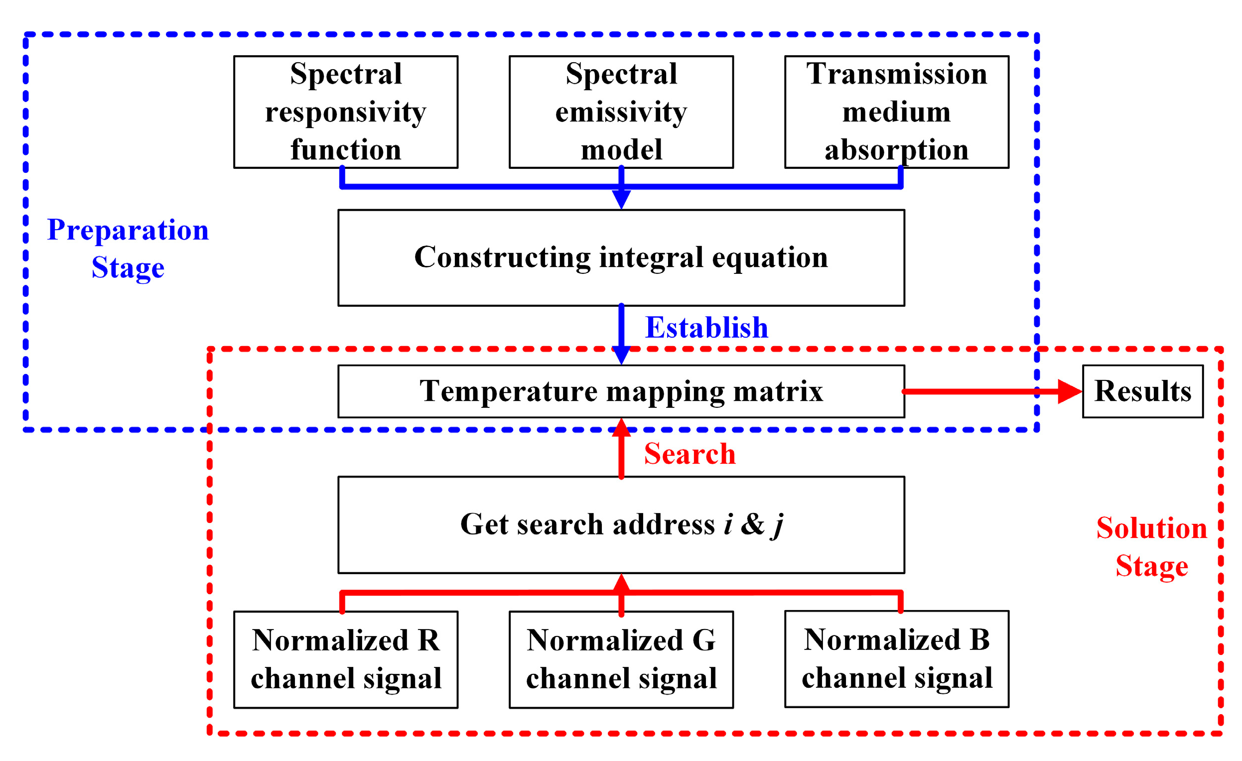
The actual temperature measurement process based on the CCD temperature measurement principle can be summarized into two stages, which are the preparation stage and the solution stage. The relationship and steps of the two stages are shown in Figure 1.
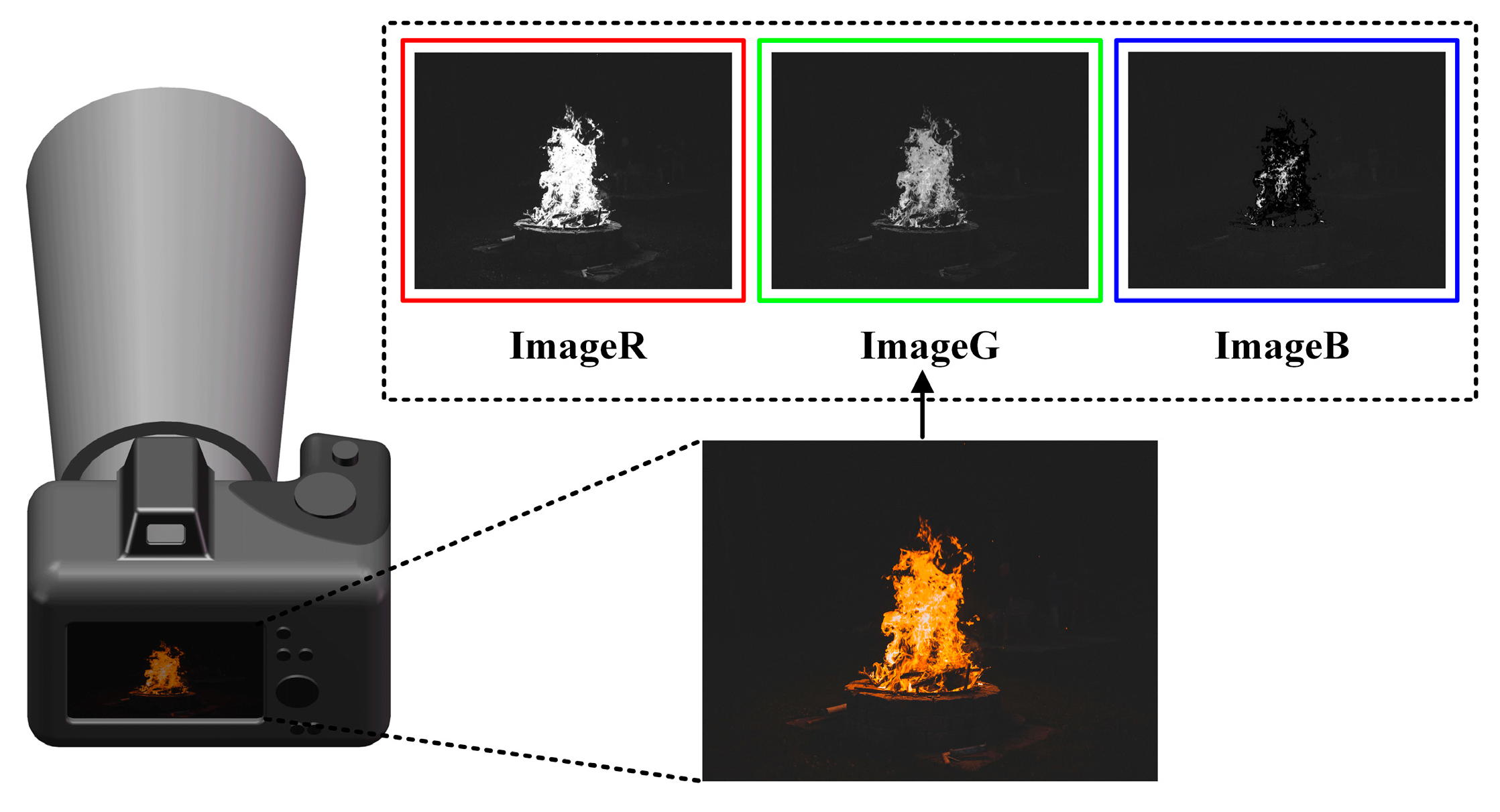
The preparation stage is marked by the blue box in the figure. This stage is completed before the measurement starts, and its ultimate goal is to generate a temperature mapping matrix for a specific temperature measurement environment. In this stage, the specific environment of temperature measurement is first determined, including the spectral response curve of the selected camera, clear imaging focal length and aperture, channel gain, emissivity model of the material to be measured, absorption model of the transmission medium and radiation transmission length, etc. Then, according to the determined temperature measurement environment, the integral equation representing the relationship between the three-channel signal and the temperature described in Formula (3) is constructed. Finally, the appropriate temperature step ΔT is set from the Draper point and substituted into the established integral equation to obtain three-channel signal values corresponding to different temperatures. The normalized three-channel signal values corresponding to each temperature are calculated by Formula (5) to obtain the distribution of temperature T in R-G space. The appropriate sensitivity factors p and q are selected by Formula (6) to calculate the channel signal step ΔR, ΔG to establish the search address. Finally, the temperature T is added to the corresponding address, and the temperature mapping Tmap is established. The solution stage is marked by the red box in the figure. The ultimate goal of this stage is to obtain the temperature solution of the corresponding position of the pixel (specific or global). At this stage, firstly, the temperature field images collected in the measurement are analyzed. As shown in Figure 2, the color images collected by the equipment are analyzed as grayscale images of three primary colors, which are stored in the form of a matrix with the same dimensions as those of the collected images. Three-channel matrices are recorded as ImageR, ImageG, and ImageB, respectively. Use Formula (5) to normalize the three-channel signal and, respectively, construct two normalized matrices ImageRnorm and ImageGnorm, with the same dimension as the image frame. The matrix elements are normalized R value and G value of the corresponding pixel, and each vector corresponds to the pixel position one by one. For the image of r × c dimension, the image normalized matrix Imagenorm is expressed as follows:
Rmn and Gmn are, respectively, the normalized R value and the normalized G value of the pixel in the m-th row and the n-th column. Then, the quotient operation is performed on the matrix element of each pixel position, and ΔRΔG is set in the preparation stage to obtain the mapping matrix search addresses I and j corresponding to each pixel as follows:
Imn and jmn are the search addresses of the temperature mapping matrix of the pixels in the m-th row and the n-th column, respectively. According to the obtained search address of each pixel, the corresponding matrix element in the temperature mapping matrix established in the preparation stage is called, and the value is the temperature calculation result of the corresponding point of the pixel. Finally, the one-to-one temperature calculation result corresponding to the pixel can be obtained, and the result is output in the form of data.
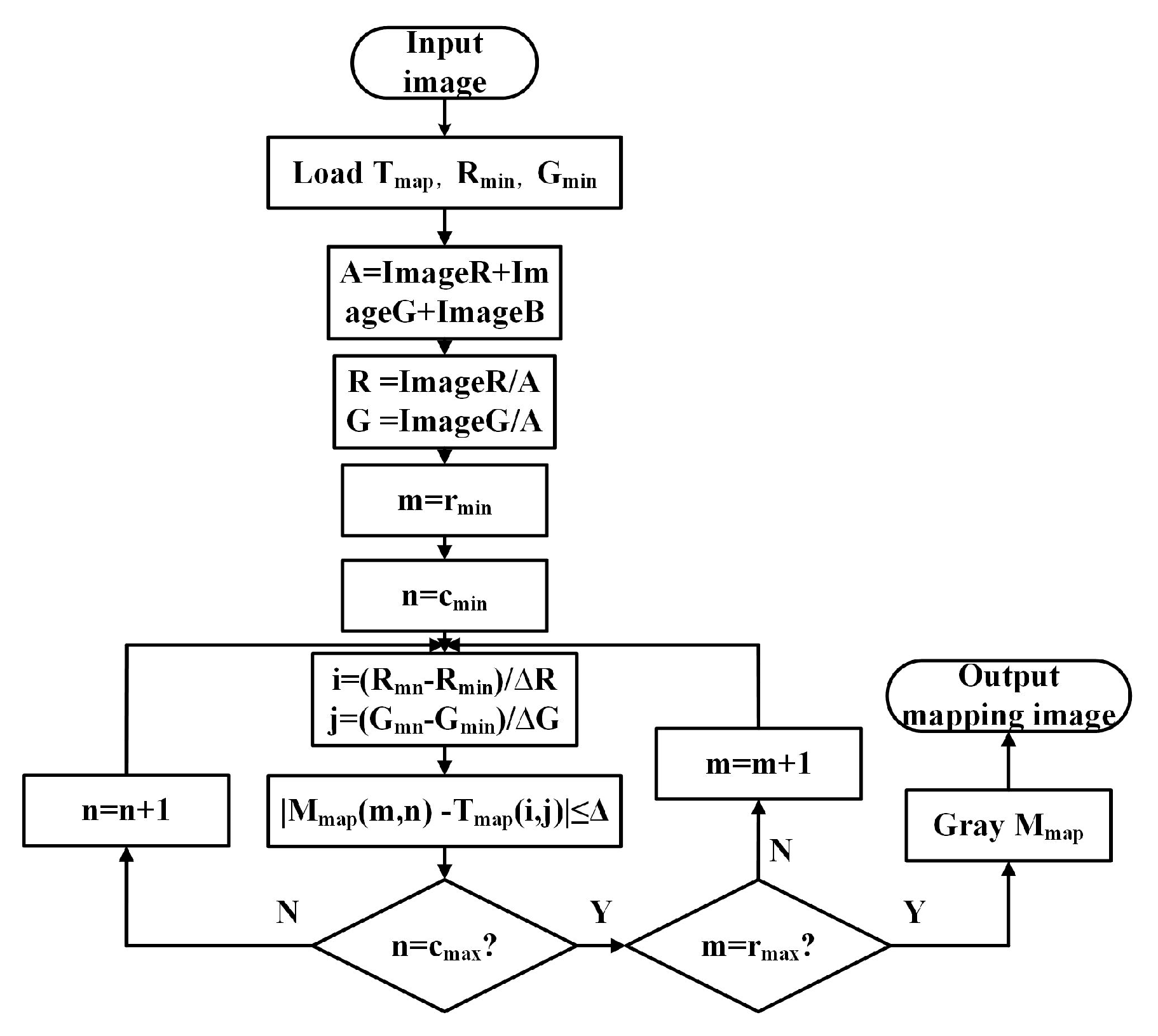
The output form of the CCD temperature measurement method based on matrix search can be divided into data type and image type. Data temperature results are mainly applied to the temperature measurement of a specific position or the temperature measurement of a small temperature field (such as the temperature field caused by a laser). This result can be obtained directly by reading the data of the corresponding pixel position. The image type result is the output spatial temperature mapping image, which can intuitively obtain the temperature distribution of the whole image or the region of interest. The output of the image type result requires post-processing of the temperature data, which is called the temperature visualization process. The block diagram of the temperature visualization program based on the matrix-seeking temperature measurement method is shown in Figure 3.
After obtaining the heat source image, firstly, the temperature mapping matrix Tmap and the minimum normalized signals Rmin and Gmin were generated in the preparation stage for this measurement into the program. Then the collected heat source image is analyzed to obtain a three-channel image matrix ImageR, ImageG, and ImageB. After the three-channel gray matrix is processed and the normalized R and G values of the image are obtained. Through two nested loop programs, the temperature solution results are assigned to a matrix Mmap which is the same as the dimension of the image frame through two nested loop programs. The loop variables m and n represent the number of rows and columns, respectively, and rmin, rmax, cmin, and cmax represent the minimum number of rows, the maximum number of rows, the minimum number of columns, and the maximum number of columns, respectively. When calculating pixels in a specific area, rmin is the starting pixel line of the area, rmax is the ending pixel line of the area, and the corresponding column values are the same. For full image calculation, the rmin value is 1, rmax is the total number of rows, and the corresponding column values are the same. After the cycle, the matrix variable Mmap corresponding to each pixel composed of temperature data will be obtained. Finally, the Mmap will be converted into grayscale data, and different pseudo-color mapping methods will be selected to obtain the temperature data visualization result.
The temperature visualization process can be well-combined with the relatively complete image processing technology. Using comprehensive image blurring, noise reduction, filtering, etc., the details of the corresponding temperature field distribution and change can be well obtained. In addition, by combining the image edge recognition algorithm, the temperature mapping region can be quickly determined, thus reducing the calculation amount of the image visualization process and effectively saving the calculation resources.
It is worth noting that this method is more inclusive in theory because it transforms the inverse problem-solving process into the forward matrix accurate searching process. It can use a more accurate emissivity model in the measurement and can well deal with the temperature measurement of multi-layer transmission media (such as air to underwater target measurement, etc.). In addition, in the process of solving, only the temperature mapping matrix and the minimum value of the normalized channel signal calculated in the preparation stage need to be stored in the memory during the solution process, which can save internal storage space.
3. Experiments
To verify the correctness of the above high-temperature measurement method, the paraffin combustion flame is used as the heat source, the standard air is used as the transmission medium, and the MER2-134-90GC camera (DAHENG IMAGING Company, Beijing, China) is used to build the temperature measurement system and carry out confirmatory experimental research. Taking the above preparation stage as a guide, this part will be developed from the following four aspects: calibration process, emissivity model selection, calculation of transmission medium absorption, and experimental situation.
3.1. Calibration Experiments
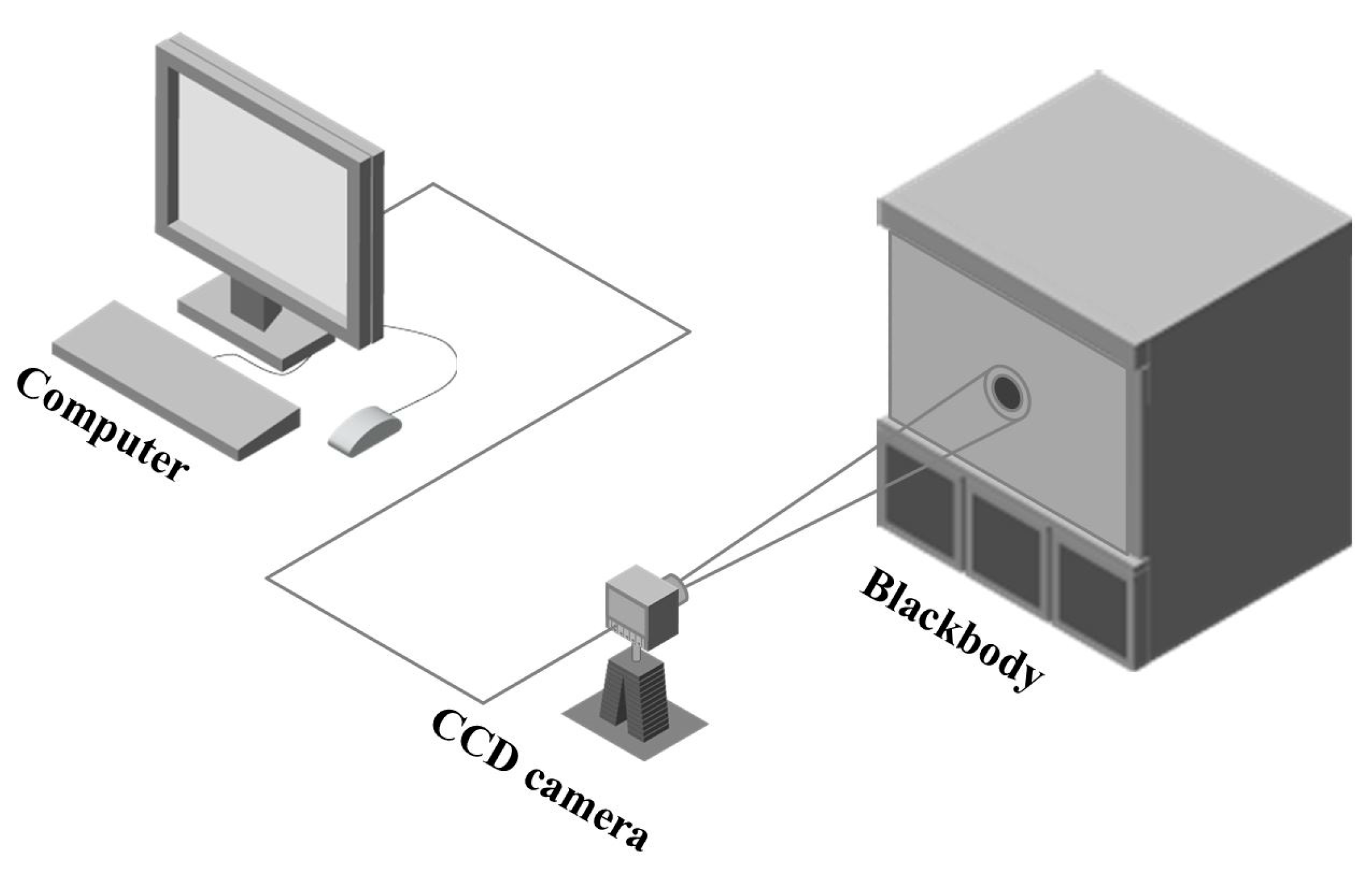
Firstly, with the lens cap installed, the MER2-134 camera is used to acquire a pure black image (lens cap image) to obtain the dark current noise D in 0–12 grayscale units existing in different pixel positions. To obtain the s current-gray conversion coefficient of the camera, the color CCD calibration method described in reference [25] is used to calibrate the MER2-134 camera with the LS1050 standard blackbody of Electro-optical Company as the standard radiation source. The schematic diagram of the experimental set-up is shown in Figure 4.
In the process of calibration, the focal length of the camera is 25 mm, the aperture is f/2.8, and the distance between the camera and the blackbody is 27.5 cm. The calibration begins when the blackbody temperature is 823 K, and then the calibration temperature increases by 50 K, and a total of 11 sets of data are obtained.
3.2. Emissivity Processing Method
In fact, under different spectral emissivity models, the same temperature can show different colorimetric values. Based on the search calculation principle of this method, reverse search based on different colorimetric values can select different spectral emissivity models in a small range.
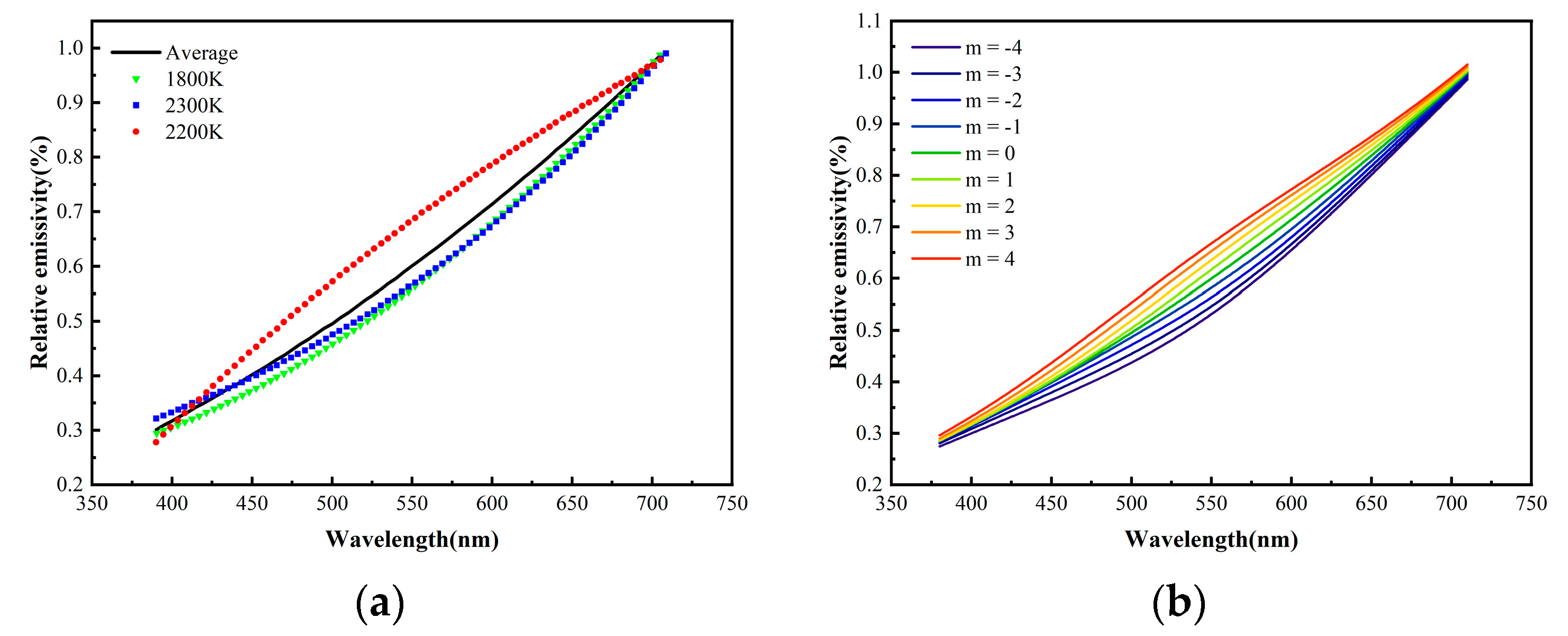
The spectral emissivity model [22,26,27,28,29] for many substances has been proposed in previous temperature measurement studies, but the temperature effect of the emissivity has not been discussed in detail. According to the actual flame spectral emissivity measurement data published in reference [30], the change of emissivity in a smaller temperature range is not linear with temperature but irregular within a certain range. Therefore, the regional spectral emissivity model is considered; that is, the region where the spectral emissivity varies with temperature is filled by introducing perturbation. The model can also verify the emissivity automatic selection ability of the method and characterize the robustness of the method.
The average spectral emissivity model disclosed in reference [30] is selected as the non-perturbative spectral emissivity, and Gaussian noise is added as the emissivity perturbation caused by temperature rise. The specific expressions of the non-perturbation emissivity model ε and perturbation emissivity model εw are as follows.
where a1 is 1.989 × 10⁻⁶; a2 is 0.002; a3 is a function of parameter m, expressed as 0.03 m; a4 is represented as λ − (580 − 15 × |m|); a5 means 5000 + 3000 × |m|; λc is the reference wavelength with a value of 710 nm. When the m value is from 0 to ±4, the perturbation emissivity model is shown in Figure 5b. It has the same range as the measured data in Figure 5a.
It is worth noting that the model is a normalized result based on the emissivity of 710 nm, while the spectral emissivity of 710 nm can be eliminated in the normalization processing of the channel signal of Equation (5), so the model can be applied to the method.
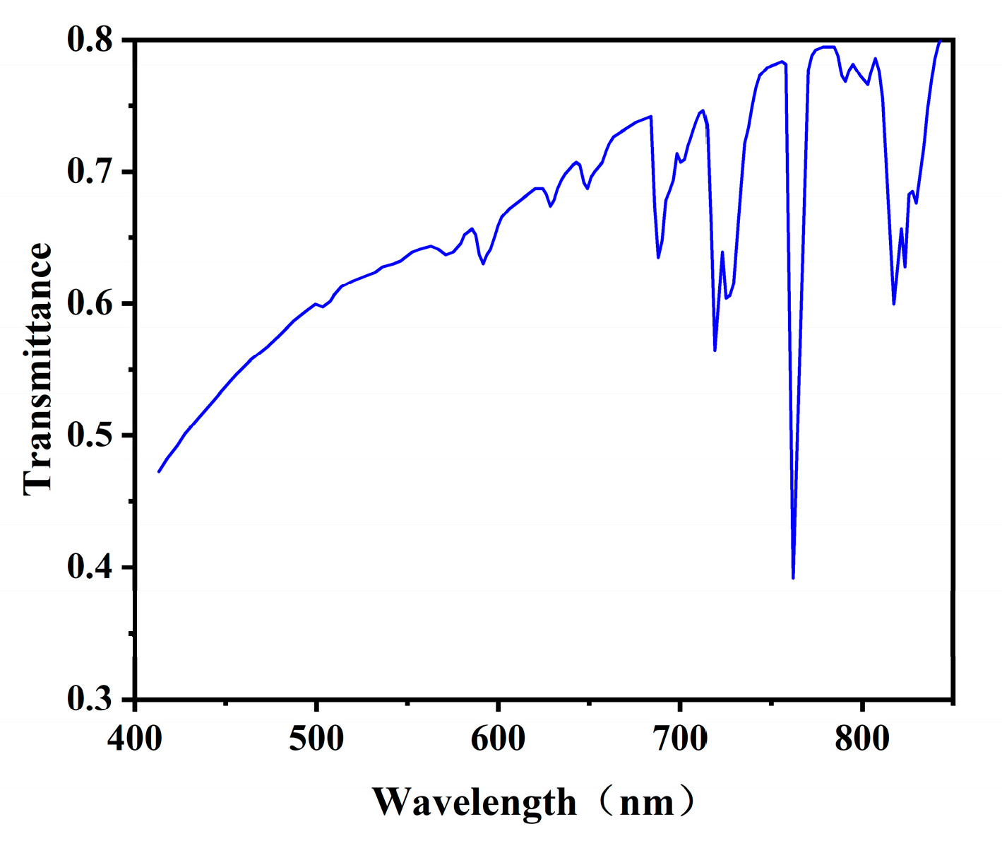
3.3. Calculation of Transmission Medium Absorption
The absorption and scattering of short-wave electromagnetic radiation by air are more intense, and the air transmittance is only 0.43 near 400 nm [31]. Therefore, in the case of long-distance temperature measurement, the neglect of the absorption of radiation signal by air will have a great impact on the calculation results. To obtain the variation of ĸ(λ), the MODTRAN® is used to calculate the air spectral transmittance under standard conditions, as shown in Figure 6.
3.4. Experimental Situation
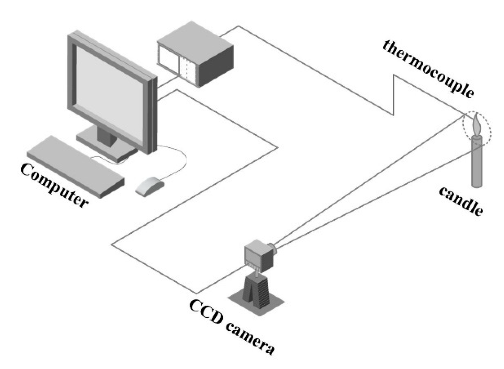
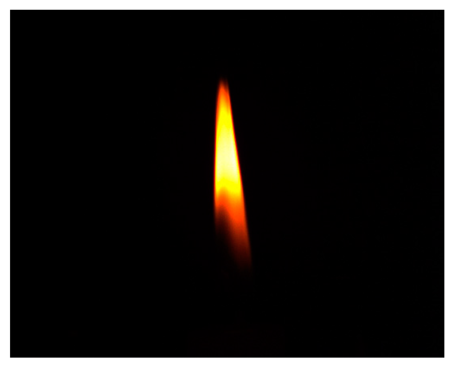
In this study, the experimental device shown in Figure 7 is set up. The calibrated DAHENG IMAGING MER2-134-90GC camera is used as the main measurement device, the platinum-rhodium thermocouple is used as the temperature check device, and the paraffin combustion flame is used as the heat source to conduct validation experiments.
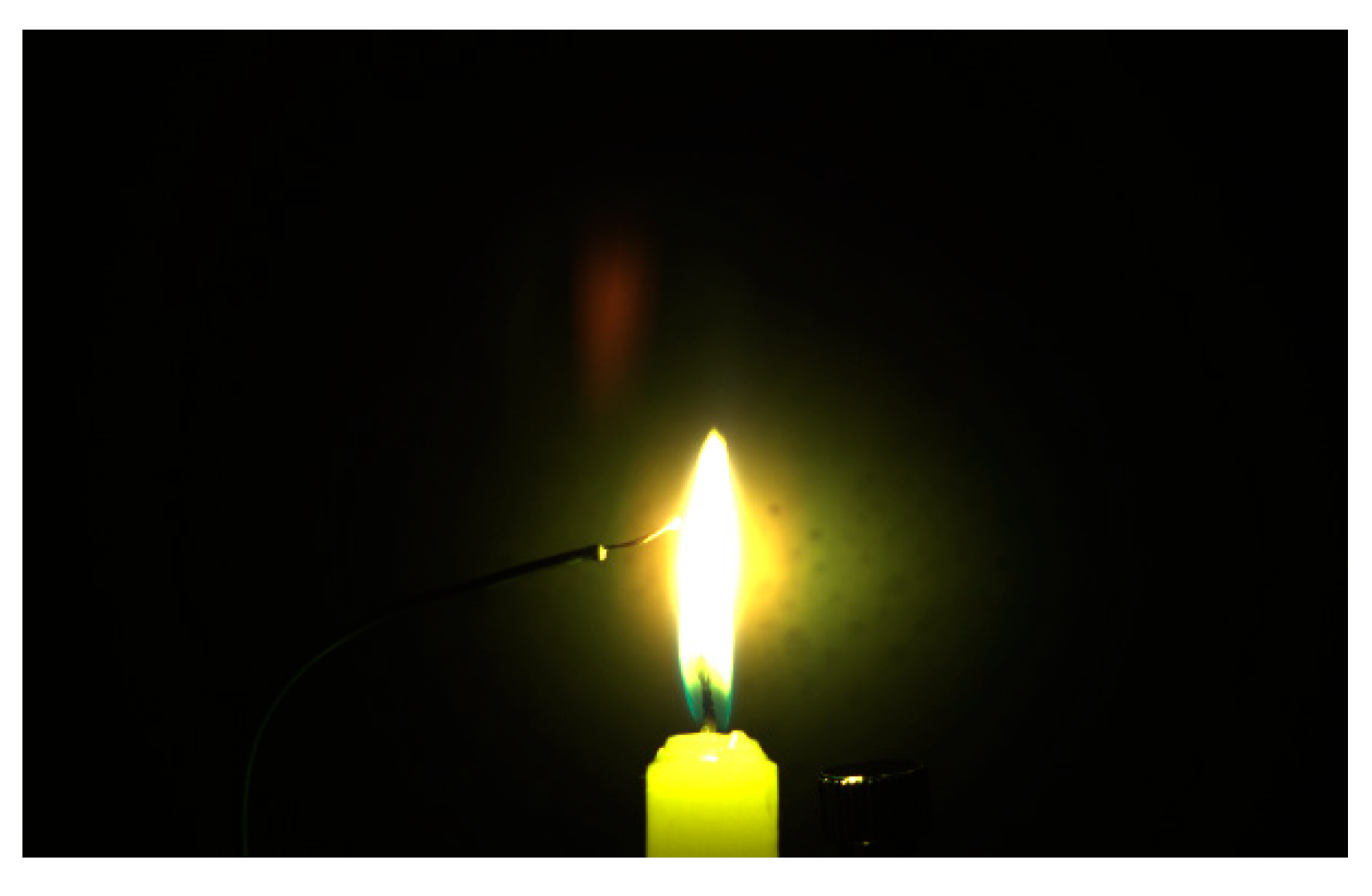
The position of the flame is located in the center of the camera acquisition, and the thermocouple is inserted into the center of the flame. The thermometer inputs the current to the thermocouple and obtains the thermal resistance at the endpoint of the thermocouple by measuring the return current and using the resistance value to obtain the temperature. The thermocouple measurement location is marked in the corresponding pixels of the camera before the experiment starts, which in this experiment is the square area surrounded by the horizontal 532–540 and vertical 370–380 pixels, as shown in Figure 8.
During the experiment, a synchronous trigger is used to link the camera to the thermocouple header, and the acquisition frame frequency of the high-speed camera and the thermocouple output frequency is synchronously set to 10 fps. Ignite the flame and start to trigger synchronously when the flame stabilizes and the flame image corresponding to the thermocouple temperature measurement data at each moment is obtained. The corresponding pixels of the point thermometer measurement position in the flame image are calculated and compared with the thermocouple data to verify the accuracy of measurement accuracy. The lens and camera parameter settings in the experiment are shown in the table.
For image temperature measurement methods, the measurement effect is directly affected by the background light. The grayscale output of the detector is proportional to the integral of the luminous flux during the exposure time, which also means that the lower exposure time can make the signal lower than the response range of the detector. In this study, this feature was used to reduce background light by using a short exposure time to reduce the luminous flux. For the temperature field to be measured, there is a quantitative relationship between the acquisition intensity and the instrument parameters in Equation (4), so it is less affected by exposure time, while the background light attenuates obviously under short exposure, as shown in the comparison between Figure 8 and Figure 9. In addition, a longer focal length is selected to ensure the clarity of the flame image acquisition. Meanwhile, a large aperture (a small number of apertures corresponding to a larger aperture) is used to make the captured image have a smaller depth of field to realize the virtual flame background, which makes the flame background intensity uniform and chromaticity single after the background light attenuation [32].
4. Results and Discussion
4.1. Calibration Results
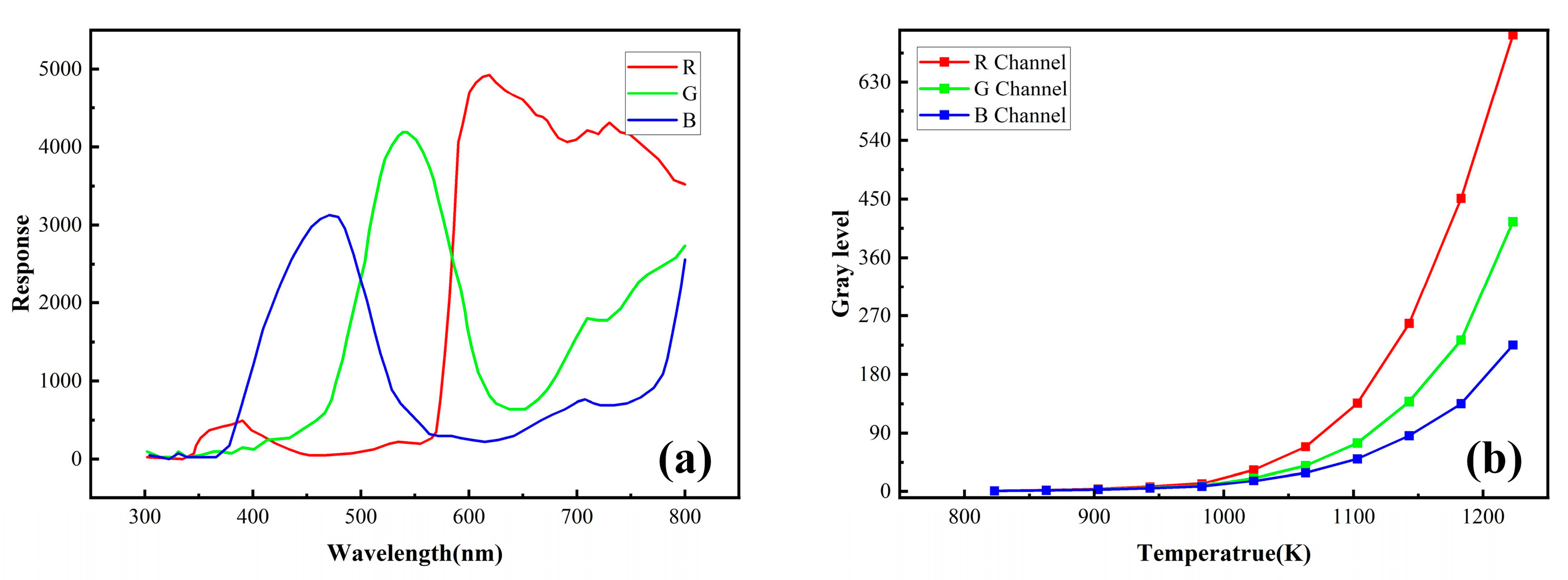
The calibration experiment has been carried out according to Figure 4. When the exposure time is 1300 us, the calibration results of the current-gray conversion coefficient and the spectral response curve of the camera are shown in Figure 10.
Figure 10a is provided by the product manual of the camera photosensitive chip Onsemi PYTHON 1300. Figure 10b shows the corresponding relationship between the output gray level of each channel and the standard blackbody temperature. With the increase in blackbody temperature, the gray change rate of the R channel is the largest, followed by the G channel, and the change of the B channel is the smallest. On the one hand, because the blackbody radiation is mainly concentrated in the long wave in the calibration temperature range, the radiation flux in the spectral range of the R channel is larger than that of the other two channels. On the other hand, the amplitude of the spectral response curve of the G channel and B channel is relatively low, which makes the intensity modulation of the thermal radiation signal more obvious, and finally forms the calibration result of the lower change rate of B and G channels.
The two sets of curves correspond to the spectral response curve si(λ) and the current-gray scale conversion factor gi in Equation (3), respectively, which will be used as the basis for the establishment of the mapping matrix and the final temperature solution.
4.2. Solution Accuracy
Combined with the experimental parameters of Table 1 and the non-perturbation spectral emissivity model in Equation (12), the temperature mapping matrix for this measurement is calculated. The p and q values of the temperature mapping matrix established in this experiment are 30 and 40, respectively. The reason is that p is the indexing of the red component, and q is the indexing of the green component. The rate of the red component rising with the radiation is higher, and the temperature range of the red component is smaller, while that of the green is relatively large in the range of 0–255. For a more uniform distribution of the temperature matrix, the case of p = 30 and q = 40 is selected to solve the problem.
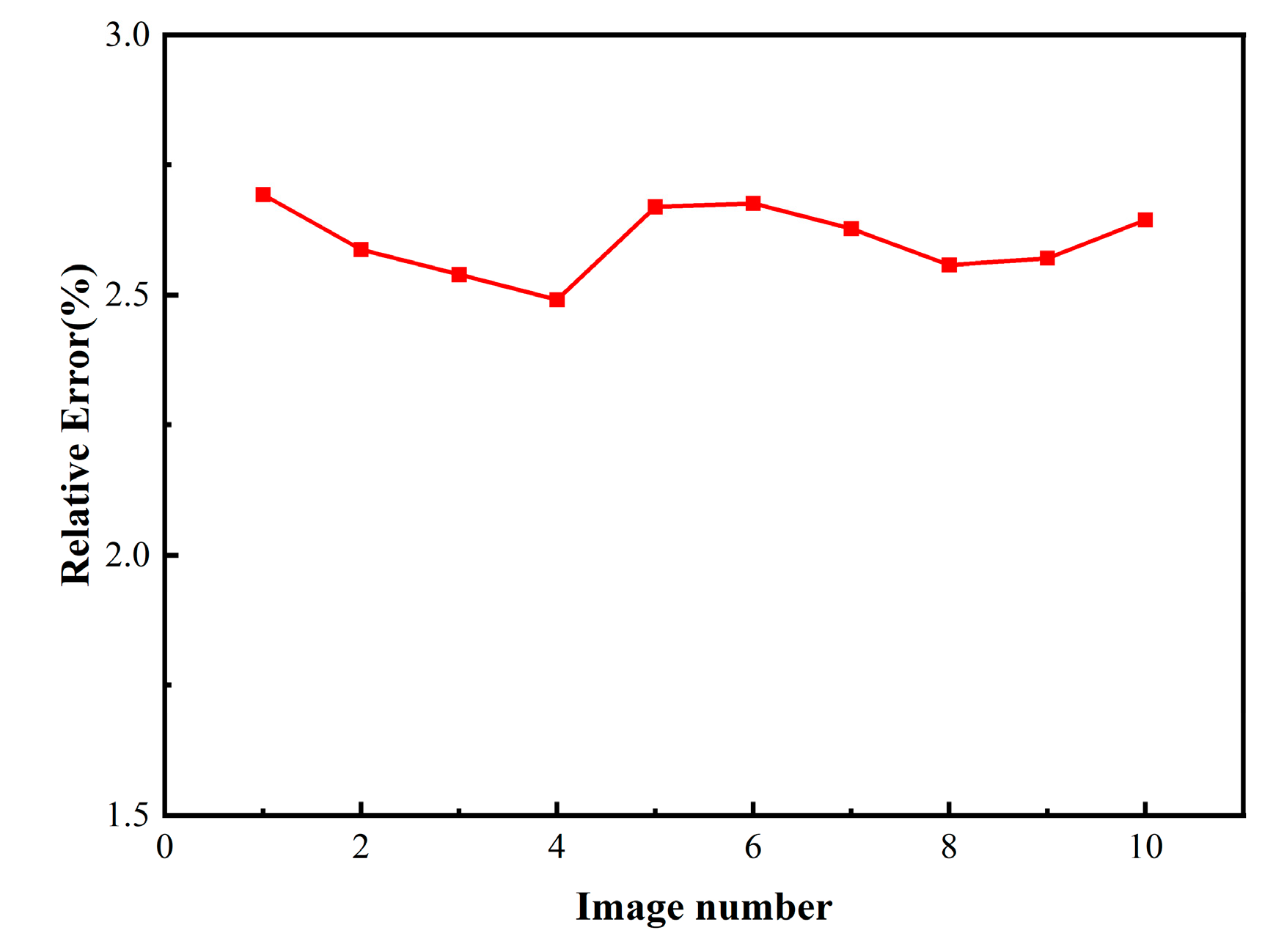
After ten consecutive triggers, the chromaticity data of 99 pixels within a specified pixel region of the image (corresponding to the pixel of the thermocouple detection position) are read, and the mapping matrix is searched to obtain the corresponding position temperature. If h is the ordinal number of pixels, N is the total number of pixels in the region, Tmea is the temperature measurement value obtained by the point thermometer, and Tcal,h is the temperature solution value of the h pixel obtained by this method, then the solution error is expressed as follows:
Equation (13) takes the average value of all the temperature solution values in the specified pixel region as the region temperature and compares it with the point thermometer measurement data of the corresponding time period to obtain the measurement error within the trigger time period. The calculation results are shown in Figure 11.
It can be seen in Figure 11 that the error of this method can be stabilized within the range of 2.5–2.7%. Considering that the measurement uncertainty of the thermocouple is 0.04%, the overall error range of the measurement is modified to 2.5% (±0.04%)–2.7% (±0.04%).
In principle, the error comes from the following three aspects: the first is the calibration data fitting error. In the calculation, in order to ensure that si(λ)ε(λ)I(λ,T) is integrable, the spectral response curve is fitted as a continuous function, which results in some measurement errors. Secondly, the spectral reflectance ignores the error. When the thermal radiation is transferred to the camera lens and image plane, part of the radiation is reflected, and the reflection is also spectral dependent. Although this point is also ignored in the calibration experiment, the spectral reflection of the lens and image plane still affects the actual temperature measurement because of the difference between the radiation behavior of the heat source and the calibration experiment. Finally, there is an error caused by the division of the minimum chromaticity interval. Because the pixels in the range of chromaticity interval ΔR and ΔG will be solved to the same temperature, the error of the solution will be caused. This error will be discussed quantitatively below.
4.3. Comparison of Emissivity Perturbation Effects
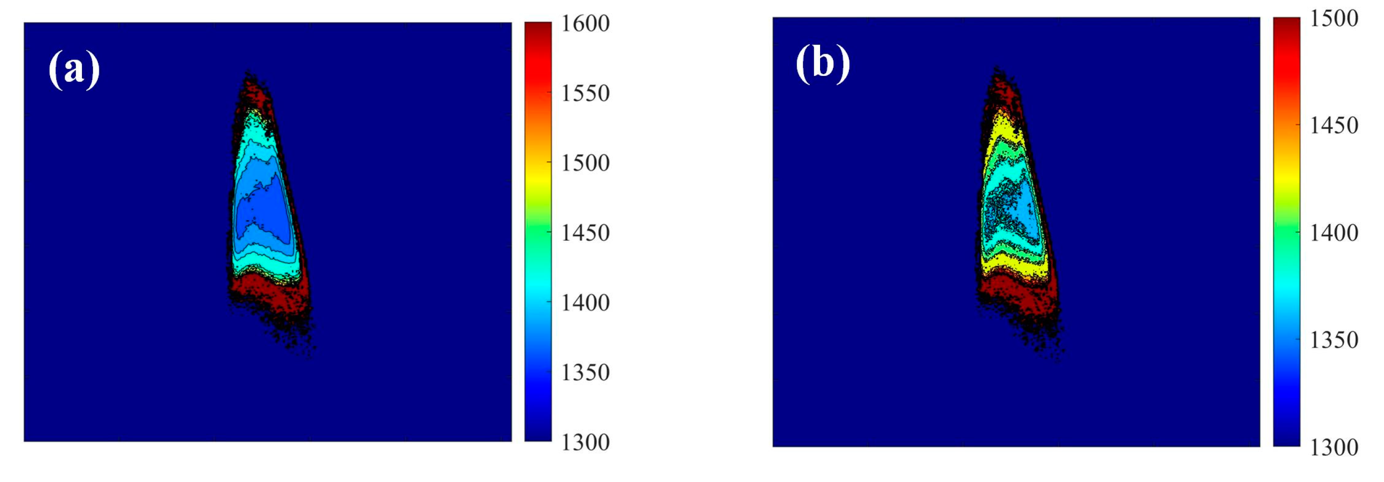
To explore the robustness of the solution method visually, the effect of temperature solution under the no-perturbation emissivity and perturbation emissivity models is analyzed according to the spectral emissivity model of Equations (12) and (13). The two emissivity models are used to build the search matrices, and the temperature mapping matrices are used to solve the non-perturbation emissivity model and the perturbation emissivity model. The results are shown in Figure 12.
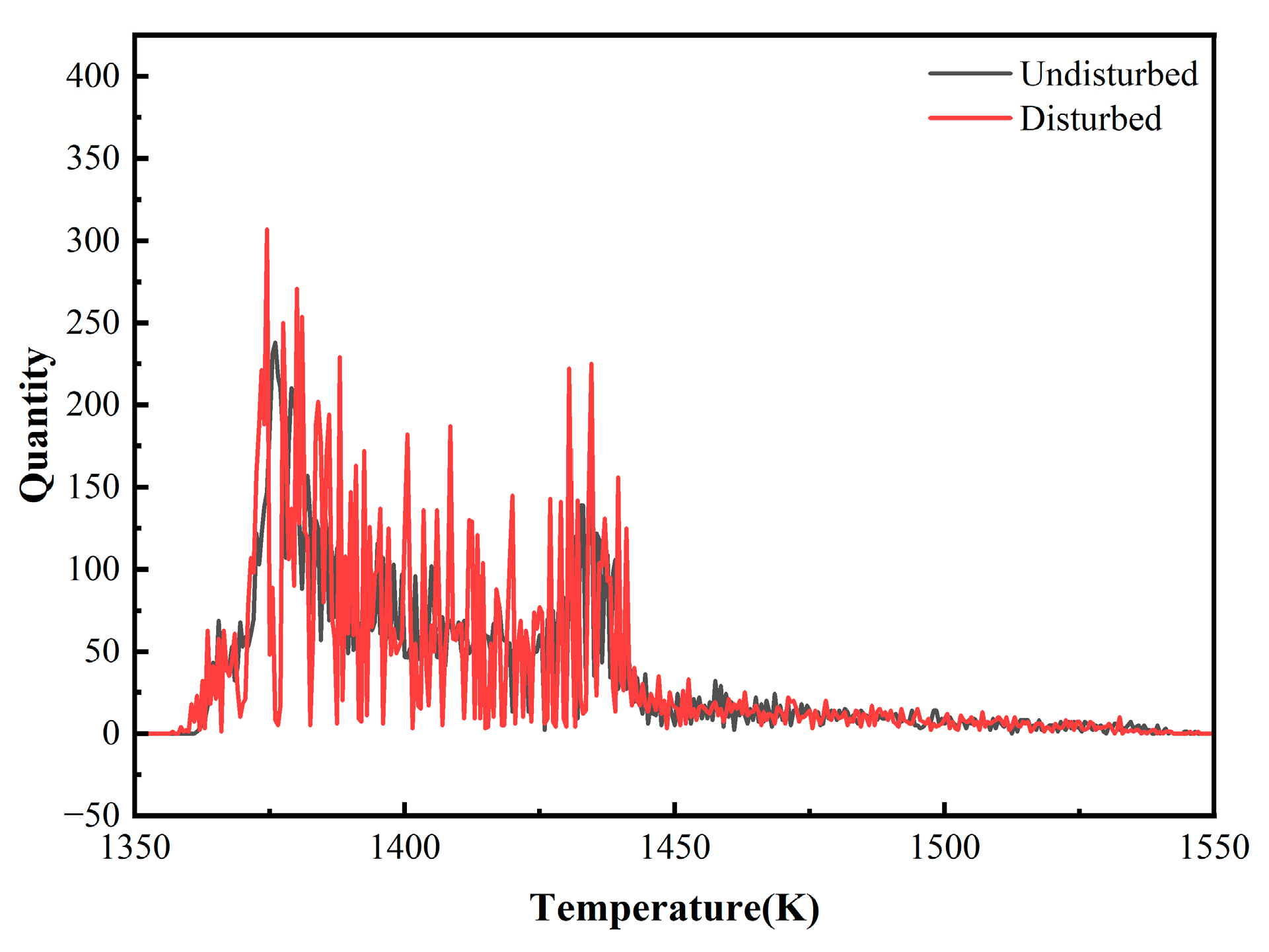
According to the solution results, both show an overall trend that the temperature of the outer flame is higher than that of the inner flame, which is consistent with the results of existing experimental studies. However, there is significant noise in the calculated results under the perturbation emissivity model, but the image has not been seriously distorted. The two-dimensional image of the solution is transformed into a statistical diagram of temperature distribution, as shown in Figure 13.
In the figure, the horizontal axis represents the temperature, and the vertical axis represents the statistical number of temperature values that appear throughout the image. It can be seen that the spectral response curve under the perturbation emissivity model has high noise and severe oscillation in the temperature range. Generally speaking, the two have the same trend. The reason for the noise may be that when solving the perturbation emissivity model, it is necessary to calculate all the emissivity models in the range and establish the search matrix. Because the model is similar, the chromaticity values at similar temperatures are similar. According to the chromaticity search, the result is calculated as a similar temperature value on different emissivity; thus, the solution fluctuation occurs.
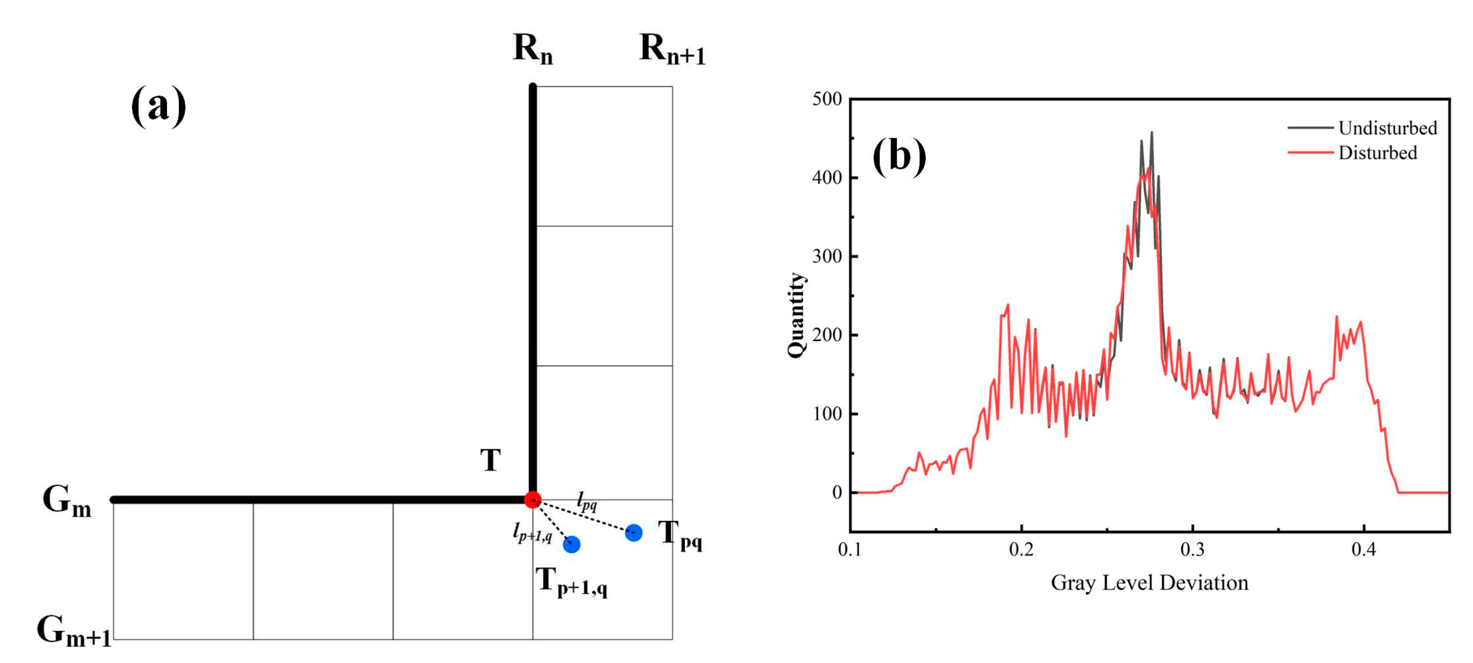
Considering that the matrix search is to calculate the temperature of the pixel points whose chromaticity falls into the determined chromaticity range as the same temperature value, the amount of deviation of the pixel points from the given chromaticity interval in the measurement is the important reason that affects the accuracy of the temperature solution. As shown in Figure 14a, the chromaticity values corresponding to the temperatures T, Tpq, and Tp+1,q will be solved at the same temperature value in the actual solution because they fall within the same divisions. However, the chromaticity of T is located at the edge of the indexing range, so its reverse search error will be minimum. Tpq and Tp+1,q are far away from the indexing boundary, so if they are classified as temperature T, there is bound to be an error, and in theory, the farther the distance, the greater the error. Therefore, the deviation distance of the measured chromaticity from the solved chromaticity is defined as the quantity characterizing the degree of error, which is denoted by l. If H denotes the three-color vector of the nearest index boundary and H′ denotes the measured three-color vector, then l is expressed as follows:
Then, to characterize the robustness of the calculation method, the statistical distribution of the deviation distances calculated in the case of perturbation spectral emissivity and non-perturbation emissivity are plotted as shown in Figure 14b.
It can be seen that the deviation distances trend of the two-emissivity models is the same, most of the positions coincide, with only a small amount of deviation at the most probable deviation distance position, i.e., where the deviation distance statistic is the largest. The perturbed emissivity model combined with the multi-emissivity model refines the search matrix. The perturbed emissivity model combined with the multi-emissivity model refines the search matrix. This also makes it possible to find a solution in which the chrominance deviation distance is smaller than that of the non-perturbative emissivity solution under the perturbation model, so the chromaticity deviation distance curve of the perturbation emissivity model is smoother. The part that not changed is the chrominance deviation distance in the process of solving the black background, so the two are the same.
According to the above experimental results, the CCD temperature measurement method based on matrix search has better temperature reduction capability. In addition, by comparing the solution results of the perturbation and non-perturbation emissivity model, the emissivity model with perturbation will introduce noise into the solution, but it has little effect on the overall solution. This indicates that the matrix searching method has strong robustness and has certain anti-interference capability.
Because of the forward calculation principle of the method, the complexity of solving the integral equation does not need to be considered, and the complex conditions such as atmospheric spectral absorption and gamma correction can be taken into account, which makes the temperature measurement closer to the real situation. In addition, only the temperature mapping matrix needs to be called in the calculation process, which can save computer’s memory and better adapt to the computer working mechanism. At the same time, because of the mechanism of fuzzy classification in the search, this method has high robustness and adapts to the actual temperature measurement conditions.
5. Conclusions
This paper proposes a color CCD high-temperature measurement method based on matrix searching, and the actual temperature inversion method is established by prior calculation. The inverse solution process is transformed into a forward mapping matrix searching process, which adapts to the working mechanism of the computer and effectively saves computational resources. The actual measurement process of the color CCD high-temperature measurement method based on matrix searching is systematically described, and the temperature visualization program is designed. The camera is used as the measuring equipment, and the paraffin combustion flame is used as the measured object to carry out confirmatory experimental research. The collected flame pictures are calculated and compared with the temperature measured by the thermocouple. The results show that the measurement error is in the range of 2.5% (±0.04%)–2.7% (±0.04%). At the same time, by comparing the solution results and chrominance deviation distance of the perturbation and the non-perturbation emissivity model, the influence of disturbance on the method is discussed. The results show that the method has high robustness and that its solution depends on forward-searching, which makes the method well-adapted to complex measurement environments and conditions and provides a new idea for high-temperature measurements.
Author Contributions
Conceptualization, C.L.; Validation, C.L. and L.G.; Formal analysis, Y.W.; Investigation, Y.W. and L.G.; Resources, D.K.; Data curation, Y.W., X.Z. and Q.Z.; Writing—original draft, C.L.; Visualization, X.Z. and Q.Z.; Supervision, D.K.; Project administration, D.K.; Funding acquisition, D.K. All authors have read and agreed to the published version of the manuscript.
Funding
This work is supported by the National Defense Science and Technology Innovation Zone Project of China (20-163-30-ZT-004-015-01).
Institutional Review Board Statement
Not applicable.
Informed Consent Statement
Not applicable.
Data Availability Statement
The data presented in this study are available on request from the corresponding author.
Conflicts of Interest
The authors declare no conflict of interest.
References
- Howell, J.R.; Mengüç, M.P.; Daun, K.; Siegel, R. Thermal Radiation Heat Transfer; CRC Press: Boca Raton, FL, USA, 2020. [Google Scholar]
- Modest, M.F.; Mazumder, S. Radiative Heat Transfer; Academic Press: Cambridge, MA, USA, 2021. [Google Scholar]
- Xiangyu, Z.; Xu, L.; Bo, Z.; Hongjie, X. Temperature measurement of coal fired flame in the cement kiln by raw image processing. Measurement 2018, 129, 471–478. [Google Scholar] [CrossRef]
- Fu, T.; Wang, Z.; Cheng, X. Temperature Measurements of Diesel Fuel Combustion With Multicolor Pyrometry. J. Heat Transf. Trans. ASME 2010, 132, 051602. [Google Scholar] [CrossRef]
- Zeng, Z.; Zhang, J.Q.; Liu, Y. Surface temperature monitoring of casting strand based on CCD image. Adv. Mater. Res. 2011, 154–155, 235–238. [Google Scholar] [CrossRef]
- Zhang, Y.; Lang, X.; Hu, Z.; Shu, S. Development of a CCD-based pyrometer for surface temperature measurement of casting billets. Meas. Sci. Technol. 2017, 28, 065903. [Google Scholar] [CrossRef]
- Zhou, H.-C.; Han, S.-D.; Sheng, F.; Zheng, C.-G. Visualization of three-dimensional temperature distributions in a large-scale furnace via regularized reconstruction from radiative energy images: Numerical studies. J. Quant. Spectrosc. Radiat. Transf. 2002, 72, 361–383. [Google Scholar] [CrossRef]
- Lou, C.; Zhou, H.-C.; Yu, P.-F.; Jiang, Z.-W. Measurements of the flame emissivity and radiative properties of particulate medium in pulverized-coal-fired boiler furnaces by image processing of visible radiation. Proc. Combust. Inst. 2007, 31, 2771–2778. [Google Scholar] [CrossRef]
- Renier, E.; Meriaudeau, F.; Suzeau, P.; Truchetet, F. CCD temperature imaging: Applications in steel industry. In Proceedings of the 1996 IEEE IECON. 22nd International Conference on Industrial Electronics, Control, and Instrumentation, Taipei, Taiwan, 9 August 1996; pp. 1295–1300. [Google Scholar]
- Simmons, D.F.; Fortgang, C.M.; Holtkamp, D.B. Using multispectral imaging to measure temperature profiles and emissivity of large thermionic dispenser cathodes. Rev. Sci. Instrum. 2005, 76, 044901. [Google Scholar] [CrossRef]
- Sutter, G.; Faure, L.; Molinari, A.; Ranc, N.; Pina, V. An experimental technique for the measurement of temperature fields for the orthogonal cutting in high speed machining. Int. J. Mach. Tools Manuf. 2003, 43, 671–678. [Google Scholar] [CrossRef]
- Fu, T.; Cheng, X.; Yang, Z. Theoretical evaluation of measurement uncertainties of two-color pyrometry applied to optical diagnostics. Appl. Opt. 2008, 47, 6112–6123. [Google Scholar] [CrossRef]
- Fu, T.; Zhao, H.; Zeng, J.; Wang, Z.; Shi, C. Improvements to the three-color optical CCD-based pyrometer system. Appl. Opt. 2010, 49, 5997–6005. [Google Scholar] [CrossRef]
- Fu, T.; Yang, Z.; Wang, L.; Cheng, X.; Zhong, M.; Shi, C. Measurement performance of an optical CCD-based pyrometer system. Opt. Laser Technol. 2010, 42, 586–593. [Google Scholar] [CrossRef]
- Qi, P.; Wang, G.; Gao, Z.; Liu, X.; Liu, W. Measurements of Temperature Distribution for High Temperature Steel Plates Based on Digital Image Correlation. Materials 2019, 12, 3322. [Google Scholar] [CrossRef] [PubMed]
- Cai, J.; Zhang, X.; Yang, Y.; Meng, S. Image Distortion and Non-Uniformity Correction for Transient Imaging Multi-spectrum Thermometry. J. Phys. Conf. Ser. 2018, 1065, 122004. [Google Scholar] [CrossRef]
- Sauer, V.M.; Schoegl, I. Numerical assessment of uncertainty and dynamic range expansion of multispectral image-based pyrometry. Measurement 2019, 145, 820–832. [Google Scholar] [CrossRef]
- Jian, X.; Rana, R.S.; Gu, W. Emissivity range constraints algorithm for multi-wavelength pyrometer (MWP). Opt. Express 2016, 24, 19185. [Google Scholar]
- Xing, J.; Peng, B.; Ma, Z.; Guo, X.; Dai, L.; Gu, W.; Song, W. Directly data processing algorithm for multi-wavelength pyrometer (MWP). Opt. Express 2017, 25, 30560. [Google Scholar] [CrossRef]
- Farid, H. Blind inverse gamma correction. IEEE Trans. Image Process. 2001, 10, 1428–1433. [Google Scholar] [CrossRef]
- Núñez-Cascajero, A.; Tapetado, A.; Vargas, S.; Vázquez, C.J.S. Optical fiber pyrometer designs for temperature measurements depending on object size. Sensors 2021, 21, 646. [Google Scholar] [CrossRef]
- Fu, T.; Cheng, X.; Zhong, M.; Liu, T. The theoretical prediction analyses of the measurement range for multi-band pyrometry. Meas. Sci. Technol. 2006, 17, 2751–2756. [Google Scholar] [CrossRef]
- Wang, T.; Peng, C.; Gang, Y. Reconstruction of Temperature Field in Coal-fired Boiler Based on Limited Flame Image Information. Combust. Sci. Technol. 2021, 195, 557–575. [Google Scholar] [CrossRef]
- Arya, S. An optimal algorithm for approximate nearest neighbor searching fixed dimensions. Soc. Ind. Appl. Math. 1994, 45, 891–923. [Google Scholar] [CrossRef]
- Zhang, Y.; Zhang, W.; Dong, Z.; Shu, S.; Xing, C. Calibration and measurement performance analysis for a spectral band charge-coupled-device-based pyrometer. Rev. Sci. Instrum. 2020, 91, 064904. [Google Scholar] [CrossRef] [PubMed]
- Draper, T.S.; Zeltner, D.; Tree, D.R.; Xue, Y.; Tsiava, R. Two-dimensional flame temperature and emissivity measurements of pulverized oxy-coal flames. Appl. Energy 2012, 95, 38–44. [Google Scholar] [CrossRef]
- Daniel, K.; Feng, C.; Gao, S. Application of multispectral radiation thermometry in temperature measurement of thermal barrier coated surfaces. Measurement 2016, 92, 218–223. [Google Scholar] [CrossRef]
- Duvaut, T. Comparison between multiwavelength infrared and visible pyrometry: Application to metals. Infrared Phys. Technol. 2008, 51, 292–299. [Google Scholar] [CrossRef]
- Alberti, M.; Weber, R.; Mancini, M.; Modest, M. Comparison of models for predicting band emissivity of carbon dioxide and water vapour at high temperatures. Int. J. Heat Mass Transf. 2013, 64, 910–925. [Google Scholar] [CrossRef]
- Xu, Y.; Li, S.; Yuan, Y.; Yao, Q. Measurement on the Surface Temperature of Dispersed Chars in a Flat-Flame Burner Using Modified RGB Pyrometry. Energy Fuels 2016, 31, 2228–2235. [Google Scholar] [CrossRef]
- Kindel, B.C.; Qu, Z.; Goetz, A.F. Direct solar spectral irradiance and transmittance measurements from 350 to 2500 nm. Appl. Opt. 2001, 40, 3483–3494. [Google Scholar] [CrossRef]
- Smith, W.J. Modern Optical Engineering, 4th ed.; McGraw Hill: New York, NY, USA, 2007. [Google Scholar]
Figure 1.
Flow chart of temperature measurement.

Figure 2.
Schematic diagram of temperature field acquisition image analysis.

Figure 3.
Block diagram of the temperature visualization program.

Figure 4.
Diagram of calibration experimental device.

Figure 5.
(a) No perturbation emissivity model; (b) perturbation emissivity model.

Figure 6.
Air spectral transmittance solution results.

Figure 7.
Diagram of the experimental device.

Figure 8.
Position identification of thermocouple.

Figure 9.
Background light attenuation effect.

Figure 10.
(a) Spectral response curve; (b) current-grayscale conversion factor.

Figure 11.
Error calculation results.

Figure 12.
(a) Results of the non-perturbative emissivity model; (b) results of the perturbative emissivity model.
Figure 12.
(a) Results of the non-perturbative emissivity model; (b) results of the perturbative emissivity model.

Figure 13.
Statistical distribution of temperature results from two emissivity models.

Figure 14.
(a) Schematic diagram of the effect of chromaticity deviation distance; (b) statistical distribution of chromaticity deviation distance of two emissivities.
Figure 14.
(a) Schematic diagram of the effect of chromaticity deviation distance; (b) statistical distribution of chromaticity deviation distance of two emissivities.


Table 1.
Table of experimental parameters.
| Parameter | Parameter Value |
|---|---|
| Lens focal length | 75 × 10−3 (m) |
| Aperture size | f/2.8 |
| Magnification | 0.5 |
| Gamma value | 1 |
| Pixel dimensions | 20 × 10−6 (m) |
| Exposure time | 300 (us) |
| Camera distance | 1 (m) |
Disclaimer/Publisher’s Note: The statements, opinions and data contained in all publications are solely those of the individual author(s) and contributor(s) and not of MDPI and/or the editor(s). MDPI and/or the editor(s) disclaim responsibility for any injury to people or property resulting from any ideas, methods, instructions or products referred to in the content. |
© 2023 by the authors. Licensee MDPI, Basel, Switzerland. This article is an open access article distributed under the terms and conditions of the Creative Commons Attribution (CC BY) license (https://creativecommons.org/licenses/by/4.0/).
Share and Cite
MDPI and ACS Style
Li, C.; Kong, D.; Wang, Y.; Gao, L.; Zhang, X.; Zhang, Q. Color CCD High-Temperature Measurement Method Based on Matrix Searching. Appl. Sci. 2023, 13, 5334. https://doi.org/10.3390/app13095334
AMA Style
Li C, Kong D, Wang Y, Gao L, Zhang X, Zhang Q. Color CCD High-Temperature Measurement Method Based on Matrix Searching. Applied Sciences. 2023; 13(9):5334. https://doi.org/10.3390/app13095334
Chicago/Turabian StyleLi, Chao, Deren Kong, Yongjuan Wang, Liming Gao, Xiangyong Zhang, and Qi Zhang. 2023. "Color CCD High-Temperature Measurement Method Based on Matrix Searching" Applied Sciences 13, no. 9: 5334. https://doi.org/10.3390/app13095334
Note that from the first issue of 2016, this journal uses article numbers instead of page numbers. See further details here.