

Time Series Forecasting Performance of the Novel Deep Learning Algorithms on Stack Overflow Website Data


1
Gendarmerie and Coast Guard Academy, Beytepe, Ankara 06805, Turkey
2
Department of Electrical and Electronics Engineering, Faculty of Engineering and Architecture, Kafkas University, Kars 36100, Turkey
*
Author to whom correspondence should be addressed.
Appl. Sci. 2023, 13(8), 4781; https://doi.org/10.3390/app13084781
Submission received: 3 March 2023
/
Revised: 31 March 2023
/
Accepted: 8 April 2023
/
Published: 11 April 2023
(This article belongs to the Special Issue The Advanced Application of Intelligent Sensor & Artificial intelligence (AI))
Abstract
:Time series forecasting covers a wide range of topics, such as predicting stock prices, estimating solar wind, estimating the number of scientific papers to be published, etc. Among the machine learning models, in particular, deep learning algorithms are the most used and successful ones. This is why we only focus on deep learning models. Even though it is a hot topic, there are only a few comprehensive studies, and in many studies, there is not much detail about the tested models, which makes it impossible to constitute a comparison chart. Thus, one of the main motivations for this work is to present comprehensive research by providing details about the tested models. In this study, a corpus of the asked questions and their metadata were extracted from the software development and troubleshooting website. Then, univariate time series data were created from the frequency of the questions that included the word “python” as the tag information. In the experiments, deep learning models were trained on the extracted time series, and their prediction performances are presented. Among the tested models, the model using convolutional neural network (CNN) layers in the form of wavenet architecture achieved the best result.
1. Introduction
Time series are seen nearly everywhere in our daily life. We can observe time series in stock prices, weather forecast, historical trends, demand graphs, heartbeat signals, etc. If we make a concise description, a time series is an ordered sequence of values that are usually equally spaced over time. In univariate series, there is only one value at each time step, and in multivariate time series, there are multiple values at each time step. Forecasting the future via time series is very popular because artificial intelligence applications such as predicting forex and stock prices have high financial potential [1]. Time series forecasting is also used for reconstructing corrupted or missing parts, which is known as imputation [2,3]. In some cases, time series analyses are also used to detect abnormal patterns. For example, in the cybersecurity field, they are used to detect abnormalities in the network traffic such as spam or denial of distributed service attacks [4]. Multi-layered neural networks, which are called deep learning methods, have been applied to various kinds of classification and regression problems. Especially in image classification tasks, they have surpassed other machine learning algorithms. One of the fields that deep learning algorithms are used for is time series forecasting. Especially, long short-term memory (LSTM) and CNN-based models are very successful in predicting the next elements of the time series [5,6,7,8].
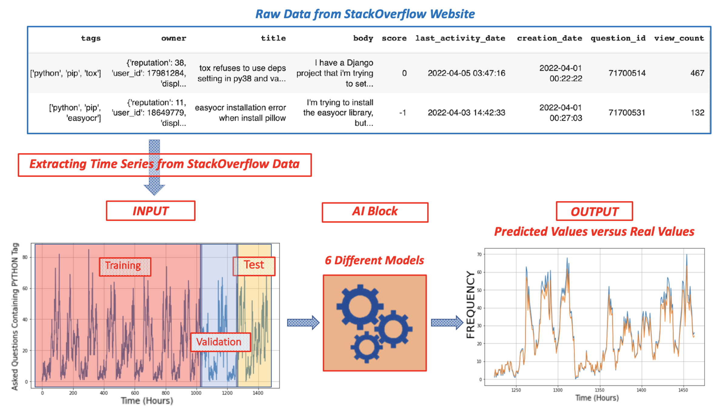
In this work, we have tested the forecasting performance of deep learning algorithms on a dataset that is extracted from the “https://stackoverflow.com/ (accessed on 7 April 2023)” website. The dataset consists of two-month long records of asked questions and corresponding information such as owner, tags, body, title, etc. This dataset consists of 32,890 rows and 10 columns. Each row represents the questions, and in the columns, information for those questions is presented. Some useful statistics were extracted from the raw dataset. This statistical information is the number of questions asked per day and hourly, the most frequently used tag groups, the most frequent individual tag item, etc. The hourly frequency counts of the asked questions are regarded as a time series and are used for the input data.
In the experiments, the input data were divided into three categories: training part, validation part, and test part. Then, a total of six different deep learning algorithms were trained and tested with the same training, validation and test sets. The algorithms belong to several groups such as simple deep models and memory models that are designed to predict time series data. After training six different deep learning models, forecasting performances were measured by using mean absolute error (MAE) metrics. According to the results, the fully convolutional CNN model outperformed other models.
2. Related Work
Forecasting the future behavior of a system can be solved by predicting time series data. Thus, predicting time series is essential and has been studied widely in various domains such as finance, climate, logistics, crime, medicine, etc. [9]. It is possible to divide the works into two main categories. The first group of works uses methods from classical machine learning algorithms based on statistical techniques. The second group of works uses deep learning models. Even though this work mainly focuses on deep learning models, it is important to emphasize traditional machine learning studies on time series forecasting since models such as support vector machines (SVM), decision trees, and other methods have been widely used before the deep learning revolution in 2012. For example, in 2003, K. Jae Kim employed an SVM model on financial time series data [10], and in 2009, L. Robert K. et al. used a fuzzy decision tree model for predicting financial data [11]. In 2004, L. Shen, and H.T. Loh used rough sets from S&P 500 data [12]. In 2015, J. Patel et al. conducted a two-phased experiment using support vector regression and random forest [13]. Another study was conducted by Zhang et al. They adopted the SVM model and multi-layer perceptron (MLP) for predicting stock price movements in China’s market [14]. In another study, the classification performance of some of the classical machine learning algorithms was evaluated on the same data, and the results are presented in [15]. Classical machine learning models are generally based on statistical theories and are used to solve the regression problem, which is the main task in time series prediction. Even though these models are used as time series predictors, they lack memorizing previous data that fail to predict and adapt to sharp changes in trends.
On the other hand, deep learning models such as LSTMs are capable of memorizing previous data and thus producing more agile predictions [16]. Even on stock data, which event-driven, lowly correlated, and unstable data, LSTM models perform well. For example, in a study conducted by Chen et al., an LSTM-based approach resulted in a 13% improvement in accuracy over classical machine learning models [17]. Another study with the LSTM model was conducted on the same dataset by Luca Di al. and yielded satisfactory results over five-day-long intervals [18]. In this work, a relatively bigger window was used for utilizing the memorizing power of LSTM architecture. Morgan B. et al. followed a similar approach as we did in this study by comparing the prediction performances of LSTM, RNN, and CNN models of three layered networks [19]. They tested deep learning models on different time series data from public datasets such as S&P 500 Daily Closing Prices stock data, Nikkei 225 Daily Closing Prices stock data, etc. According to their findings, an LSTM-based model that consisted of one bidirectional LSTM layer, followed by a dropout layer and fully connected layer, outperformed other models.
Financial time series forecasting studies constitute the majority of the research. Studies have been conducted on various data such as stock prices, bond prices, forex prices, cryptocurrency prices, etc. Most of the studies use price data as the only input, while some studies use price data and financial news data together [8]. These studies use hybrid deep learning models by combining memory cells, such as LSTM, and natural language processing (NLP) methods, such as BERT, word2vec embedding, etc. [20,21]. LSTM and variations of LSTM models dominate the financial time series forecasting studies. These text-mining hybrid works are aimed at solving financial time series problems that naturally consist of event-driven patterns. Thus, adding some textural information from financial news by using NLP techniques helps to increase the accuracy of predictions. To increase the accuracy in financial time series prediction is to using hybrid models in a single network. For example, Liu et al. applied CNN and LSTM [22], and Batres et al. combined deep belief networks (DBNs) and MLP [23].
Another important study area in time series prediction is the evaluation of multivariate time series. Likewise, we can observe multivariate time series ubiquitously in everyday life. If there is no correlation between the components of the multivariate time series, then the extra dimensional information does not contribute much to the prediction performance. Thus, in this case, univariate and multivariate predictions produce fairly similar results. Neural networks and deep learning models have also been applied to multivariate time series. For example, in a study conducted by Kang W. et al., real-world datasets, traffic data and solar energy data were analyzed with multiple CNN models [24]. the traffic dataset had two different sensors, and the solar energy dataset had information from 137 power plant. According to the experiments, multiple CNNs performed better than similar time series model such as the LSTM. In a study conducted by Lian et al. on pre-processing, principal component analysis was used on the original multidimensional input. Then, pre-processed data were used for prediction purposes [25]. Yuya Jeremy O. et al. proposed a new method by transforming original multivariate data into a higher tensor network [26].
Detailed information about the used algorithms is presented in the Methodology and Experiments section, but to provide preliminary information for the algorithms, some literature knowledge is also presented in this section. The MLP is the basis of deep learning since it consists of a basic unit called the threshold logic unit (TLU). The TLU computes a weighted sum of its inputs and then applies a step function to that sum and outputs the result.
MLP architecture consists of three layers: one input layer, some TLU units called hidden layers, and a final output layer of one TLU unit. For a long time, it was believed that the TLU unit is only capable of solving linear problems until the discovery that using a derivable activation function makes it possible to override these limitations [27]. In the literature, MLP models are highly studied, and some modified versions are proposed. For example, a study conducted by Robert R. investigated how performance is affected while using different activation functions other than step functions [28]. MLP is a supervised model, which means it requires classified data. However, it is possible to use MLP models in a supervised manner by modifying the usage architecture. In a study conducted by Ankita C. et al., to represent the usage of MLP in an unsupervised scenario, input features are mapped to an output cluster node based on the degree of belongingness [29].
The other three models studied in this work belong to RNN and LSTM architecture which are also called “memory” models, as they take information from prior inputs to influence the current input and output. These models are designed to process sequential data such as language data or time series data. The core of these kinds of algorithms is the RNN. RNNs can only memorize a limited time frame. Thus, there are many studies on making RNNs more efficient. LSTMs are among one them, and LSTMs are modified versions of RNNs designed to memorize previous information. In another study, RNN was extended to a bidirectional recurrent neural network (BRNN). The study showed that BRNN can be trained without the limitation of user input information up to a preset future frame [30]. Generally, BRNNs and Bi-LSTMs use different configurations and activation functions, but they are both effective in predicting real-life time series data [31,32].
Another method used in this work is CNN architecture, which is inspired by the convolution operator widely used in electronic engineering. CNNs are very effective, especially on image classification tasks. There are several different configurations of CNNs, such as differential convolutional neural networks, wavenet, etc. In one study conducted by M. Sarıgul et al., mathematical differentiation operation was used in the convolutional process to increase its accuracy without changing the filter numbers [33]. Wavenet is another configuration of CNN that uses a dilation factor in each layer. Wavenet is generally used in speech synthesis and voice conversion tasks, but it can also deal with various kinds of sequential data such as ECG heartbeat signal or wind speed [34,35].
3. Motivation and Contributions to the Literature
In summary, in the literature, there are different kinds of deep learning models, but the most used and successful models are MLP, RNN, LSTM, CNN, DBNs, and autoencoders [36,37]. Throughout the literature, financial time series forecasting is the most used data since this problem is investigated by the finance industry, individual investors, and academia, and experiments have been conducted by using various deep learning environments such as Tensorflow, Keras, Pytorch, Theano, and Matlab [8]. Some researchers claimed they used Python, but they do not provide detailed information about the development environment and model architecture, which makes it impossible to present a full comparison chart. Thus, for us, one of the main motivations is to constitute a study that presents the prediction performance of popular deep learning models by clearly stating the model’s architecture, development environment, and corresponding codes.
The main contributions of this paper can be summarized as follows:
- Although deep learning models have been widely used for trend prediction and time series forecasting tasks, there are only a few comprehensive studies that present the performance comparison of the models. Moreover, the works in these reviews do not provide enough information for a proper comparison. Thus, in this study, we present some literature for time series forecasting and investigate the effectiveness of the most used deep learning models on univariate time series data with the same or similar complexity models.
- Long short-term memory networks and recurrent neural networks are the kinds of networks designed to memorize previous samples. They are the most used models in time series prediction tasks and are known as the silver bullet for this kind of task. However, we present that wavenet-based CNN models can also extract useful knowledge from datasets with the dimension of time and yield producing more precise prediction results than LSTM models.
4. Dataset
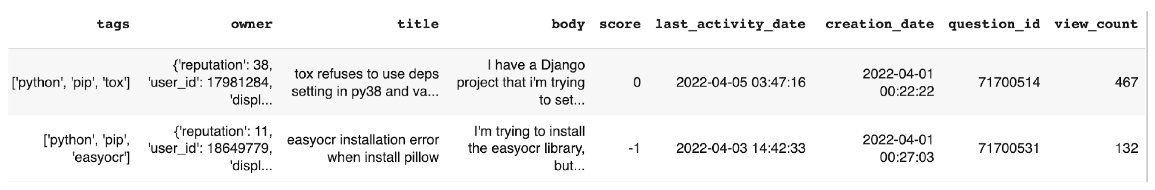
The dataset was acquired through the Stack Overflow website’s API and was saved as a comma-separated file. The dataset has 32,890 rows, and this number represents the total number of questions asked between 1 April and 31 May 2022. There are ten columns as shown in Figure 1, these columns include the information: tags, owner, title, body, score, last activity date, creation date, question ID, and view count.
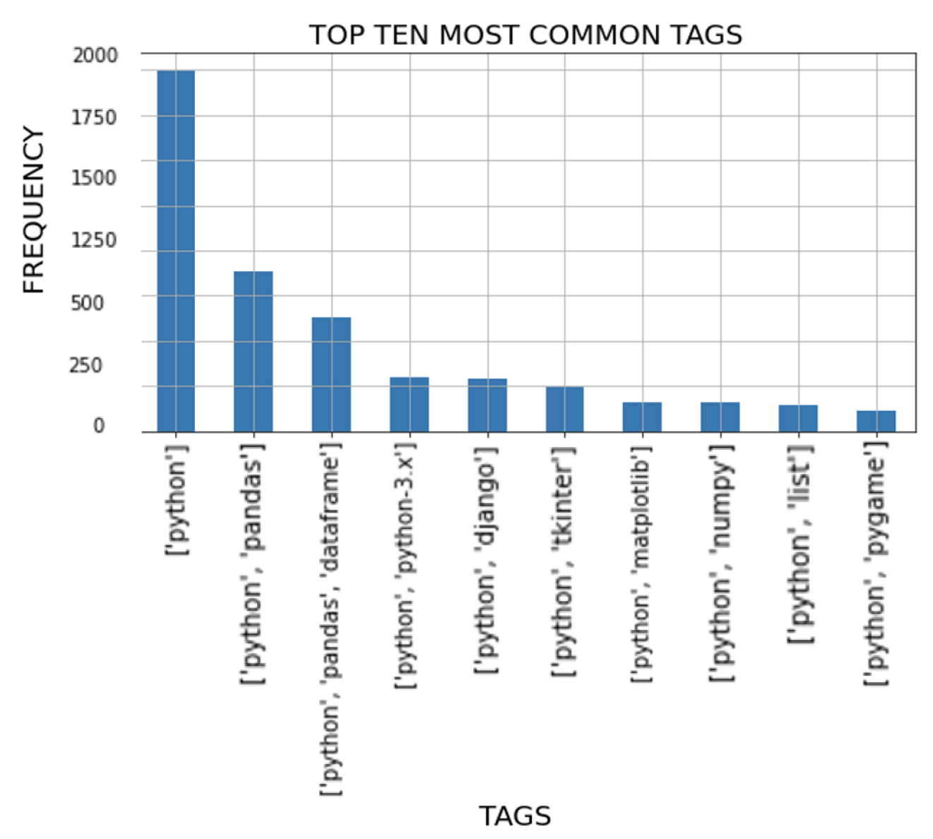
In the pre-processing part, the downloaded coma separated file was processed by using the pandas.DataFrame property. First, the dataframe was checked for duplicate or missing data. To extract a time series from the data, some useful statistic values were computed, such as density distribution of tags and number of asked questions on an hourly, daily, weekly basis, etc. According to this examination, the most popular tag groups are presented in Figure 2. The most frequent tag element was “python”, and it occurred not only as a single tag value but also inside multiple-valued groups such as “python, pandas”, “python, pandas, dataframe”, “python, django”, etc. Thus, to create time series data, a number of the asked questions with the tag value “python” were extracted. Hourly frequency of the asked questions containing the python tag is suitable to use as a time series since it is independent and identically distributed data that naturally occurs by random users of the website.
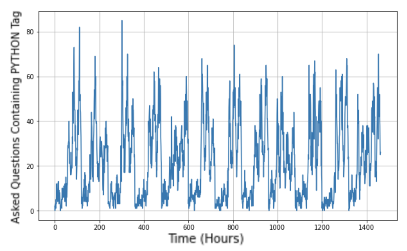
Thus, the number of asked questions containing the “python” tag is presented in a time series data format, as seen in Figure 3, and this extracted data were used for comparing the prediction performance of state-of-art deep learning models.
5. Methodology and Experiments
To provide a holistic viewpoint about the methodology followed in this study, a flowchart is presented in Figure 4.
The time series data had 1464 samples for 61 days. The first 984 samples were kept for training, and this is nearly equal to 67% of all the samples. The following 240 samples were kept for validation purposes, which are very important for mitigating the overfitting effect [38,39]. The last 240 samples were used for performance tests of all the algorithms. The test part of the dataset was used to measure the forecasting performance of the algorithms, and these data were been used before. In the scope of this work, novel deep learning models that are highly applied in time series prediction tasks were used [40]. They were: the multi-layered dense model, simple recurrent neural networks (RNN), stateful RNN, LSTM, and CNN. Among the tested models, the LSTM and CNN-based models performed especially well since they are designed to work on sequential data. All the models are implemented in Google’s Colaboratory environment, which is a cloud service for machine learning and artificial intelligence computations. It utilizes python and all major python libraries, such as TensorFlow, scikit-learn, and matplotlib, among many others, which are pre-installed and ready to be imported. Another powerful feature of Colaboratory is that it can provide GPU acceleration. As a result, Colaboratory can help to train very deep networks; otherwise, it is impossible to train such networks in ordinary computers.
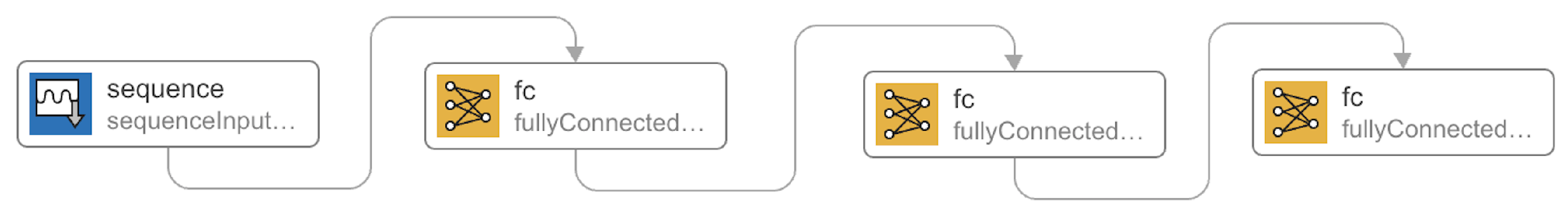
5.1. MLP Model
The first model is an MLP model consisting of dense layer units of Keras API. The first model is shown in Figure 5. Dense layers are the basis of the deep learning process, and they rely on gradient descent [41]. The theory behind gradient descent can be defined as: for each epoch, the algorithm first makes a prediction and measures the error, then goes through each layer in reverse to measure the error contribution from each connection, and finally slightly tweaks the connection weights to reduce the error.
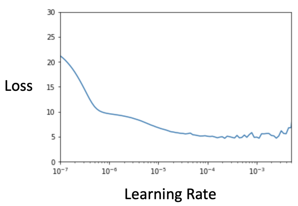
The Huber loss function of the tensorflow.keras API was used. To mitigate the overfitting effect, the “EarlyStopping” callback parameter was also used. To determine the optimal learning rate, the model was trained for 100 epochs, with different learning rates in each epoch. The change in the loss value against different learning rates is shown in Figure 6. Somewhere between 0.0001 and 0.00001 is suitable for the optimal learning rate value.
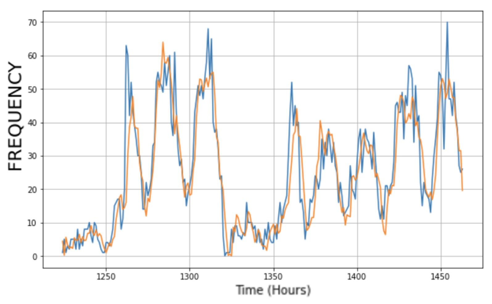
The first layer accepts 30 samples as input, and all 30 tensors are fully connected with the first layer’s 10 neuron units. The second layer accepts the first layer’s output, which is 10 tensors, and it connects those tensors with its 10 units. The last layer accepts inputs from the previous second layer and outputs only one result as the predicted number of asked questions for the next sample. The predictions of the dense model are shown with an orange line in Figure 7, and the blue line represents the real numbers of the asked questions. The dense model achieved a forecasting performance of 5.572 MAE.
5.2. RNN Model
The second model tested in the scope of this work was an RNN model. RNN models can successfully deal with sequential data, because RNN units are designed to memorize previous states [42]. This memory property was used in the computation of the current state. Thus, RNN units accept two inputs: previous output and current input value. The working mechanisms behind RNN units can be formulated as (1).
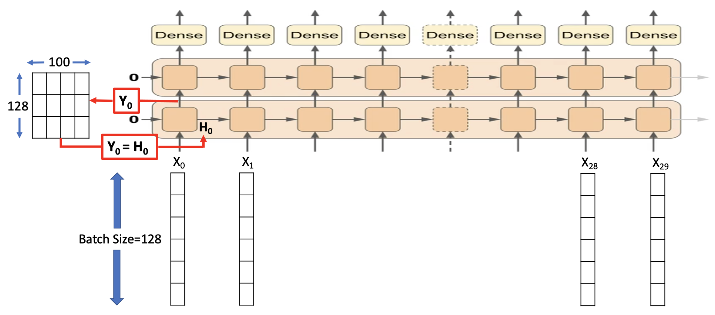
where is the current input, is the current output, and is the past output. The function that models this relation is represented by . In the case of RNN, the function is a simple hyperbolic tangent function that introduces nonlinearity since it has a tendency to have unstable gradients. Using a non-saturating activation function such as the rectified linear unit function causes gradients to grow arbitrarily large. The RNN model is implemented using the “SimpleRNN” function inside the tensorflow.keras.layers API. In this model, two recurrent layers and one dense layer were used, as shown in Figure 8.
The recurrent layers accept a batch size of 128. Each recurrent layer has 100 units, and there are 30 time steps for each. The dense layer accepts the recurrent layers’ outputs and produces a single value as the predicted number of questions. For each window, RNN runs with an initial state value of zero. Then, the state value is updated at each time step until RNN makes its prediction. If not inferred otherwise, SimpleRNN function in tensorflow.keras API clears the state value after a prediction is made and does not keep the state value for the next iterations. This configuration is known as the stateless RNN. In the stateless model, batches can randomly be chosen from the datasets, and they can even overlap each other. On the other hand, in a stateful model, batches should be chosen consecutively, and they should not overlap.
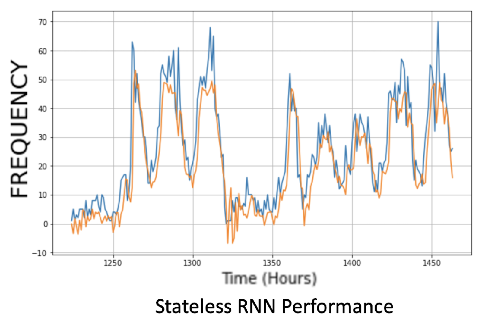
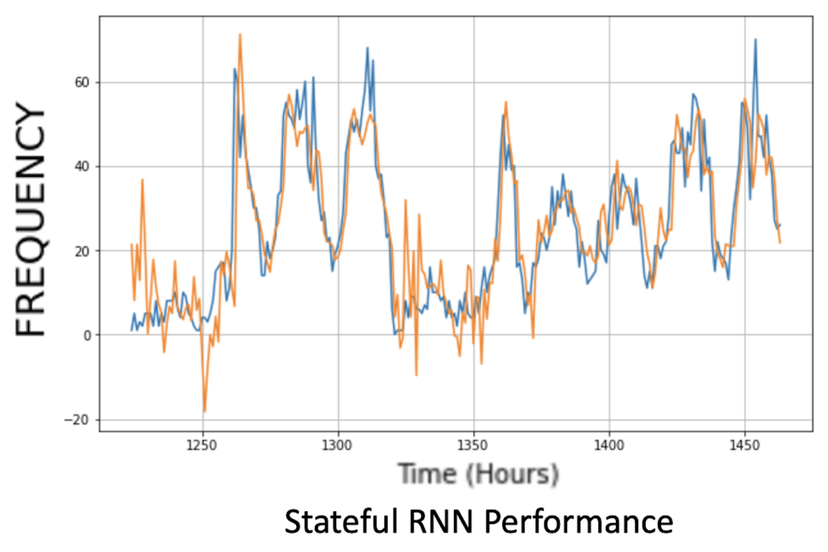
Another configuration is known as the stateful model. In this architecture, RNN units keep the state information and transfer it to the next iterations. Stateful RNN models perform better on longer sequences, but they require a longer training time, and sometimes they perform poorly because consecutive batches are highly correlated. Forecasting performance of the stateless and stateful versions are presented in Figure 9 and Figure 10, where orange lines are the predicted values and blue lines are the real numbers. The stateless RNN model performed better than the stateful RNN, but both performed worse than the dense model. The forecasting performance in terms of MAE was 6.679 for stateless RNN and 7.039 for stateful RNN.
5.3. LSTM
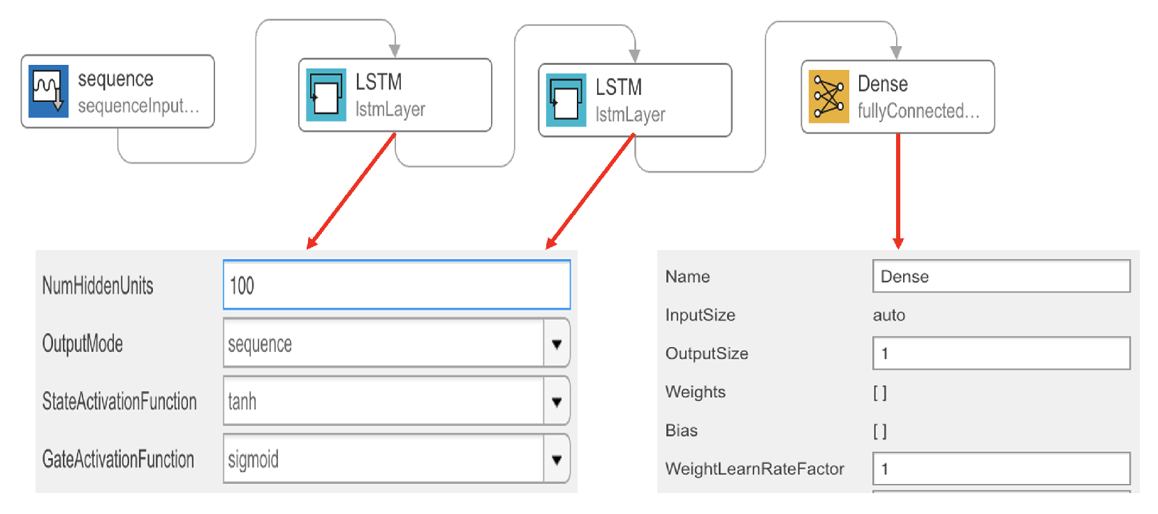
The LSTM model that is used in this work is presented in Figure 11. The model has two LSTM cells with 100 units and one dense layer. For the gates, the sigmoid activation function was used, and for the state vector, the hyperbolic tangent function was used.
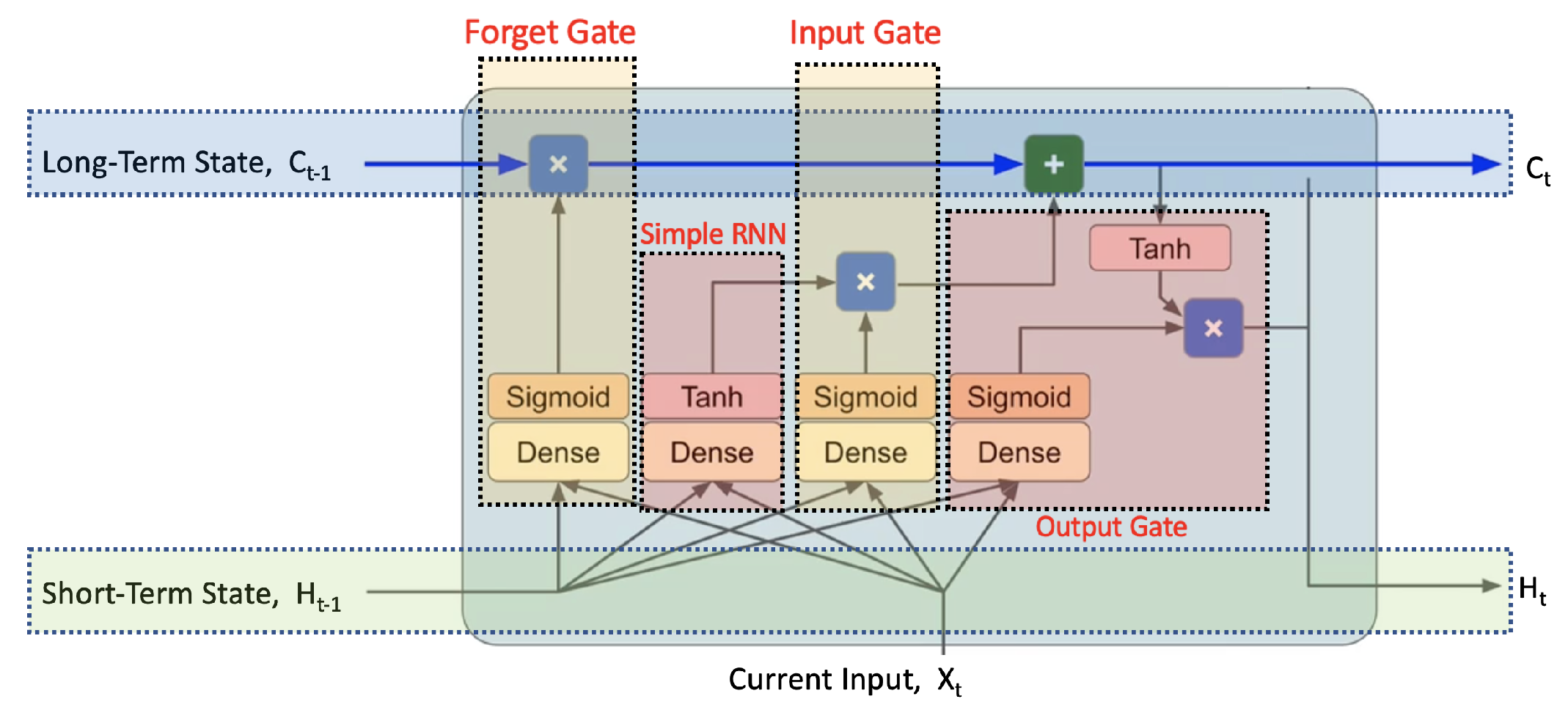
Even though recurrent networks are good at dealing with sequences, they cannot memorize long sequences. To mitigate this downsize, LSTM networks, which are a kind of variant version of RNN networks, are used. Because of the recurrent configuration of the RNN models, when the number of time steps increases, it causes a vanishing gradient problem [12]. The LSTM architecture is shown in Figure 12, and it provides an efficient way for the gradients to backpropagate.
LSTM models are more complex than RNN models, but they can deal with longer sequences, such as several hundred time steps; thus, they can produce successful results on language models [43]. As seen in Figure 12, short-term memory is conveyed with a simple RNN cell, and long-term memory is preserved with a dense layer using a sigmoid activation function and two units, forget gate and input gate. Forget gate takes the previous state vector and current sample as input. It produces values between one and zero since it uses the sigmoid function. If forget gate outputs values close to one, long-term memory is kept, but if it outputs values close to zero, long-term memory is erased. The input gate also produces values between one and zero, and the product is multiplied by the RNN cell’s output. If a trend is detected in the current input that has not existed before, the input gate decides to add this information to long-term memory. Finally, the output gate produces the result of current time steps by multiplying long-term memory with a dense layer. Forecasting performance of the LSTM model is presented in Figure 13, where orange line is the predicted values, and the blue line is the real numbers. The LSTM model has a forecasting metric of 5.375 in terms of MAE. As a result, the LSTM model performed better than the RNN models and dense model.
5.4. CNN
Convolution is an operator that slides one function over another to measure the integral of their element-wise multiplication. For example, for an input vector of “x” and the filter of “w”, which uses the rectified linear unit function (ReLu) and has a kernel size of three, the first output of the convolution is computed as shown in Equation (2). For the second, third, and other elements of the convoluted output vector of “y”, this process is repeated by sliding one element of the input vector in each step.
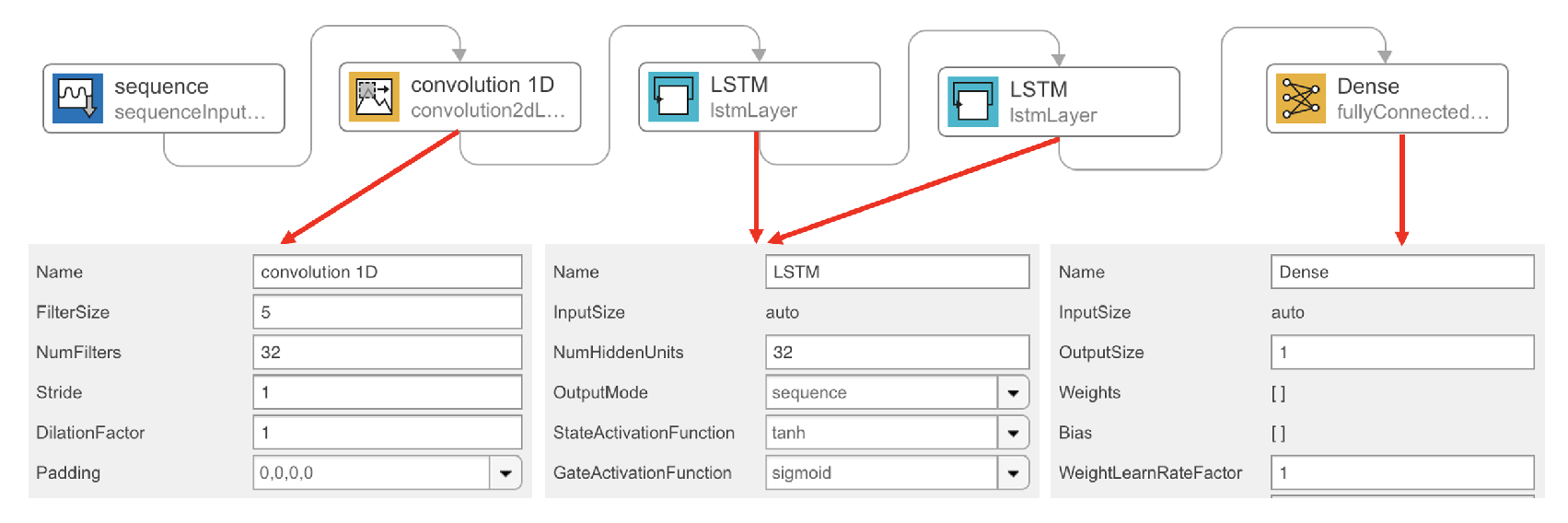
CNN is one of the widely used techniques in the field of image recognition and classification [44,45]. Convolutional layers have been successfully applied to time series prediction tasks [46,47]. In the scope of this work, two CNN models were configured, and the first model is a hybrid version of CNN and LSTM layers that is shown in Figure 14.
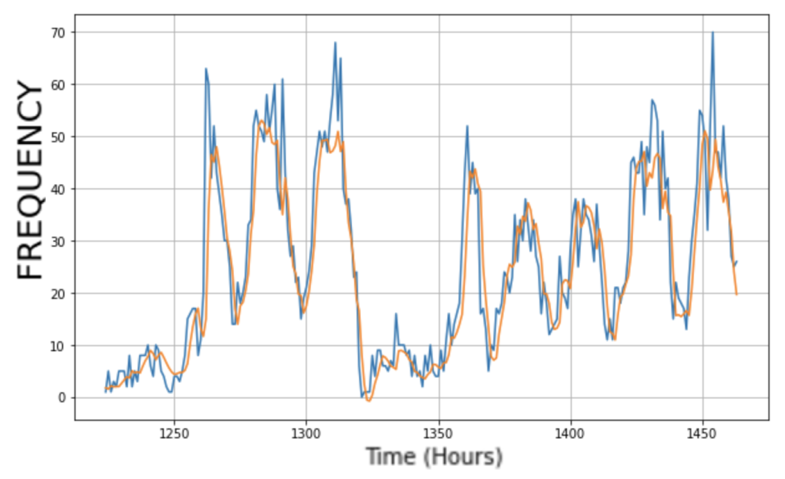
In the hybrid CNN model, convolutional layer was used like a pre-processing unit for LSTM layers. The kernel size of the CNN layer was five, and the stride parameter was set to one. The padding parameter of the tensorflow.keras API was set to “casual”. This parameter adds enough zeros at the beginning of each sequence. As a result, the output dimension will be the same as the input dimension, and the output values will be inferred only from the current and past input values. LSTM layers have 32 hidden units. The hyperbolic tangent function was used for state vectorsm, and the sigmoid function was used for the gates. The final layer was a dense layer that outputs only one value for the predicted number.
The forecasting performance of the hybrid model is presented in Figure 15, where the orange line is the predicted value, and the blue line is the real numbers. The hybrid model has a forecasting metric of 5.389 in terms of MAE.
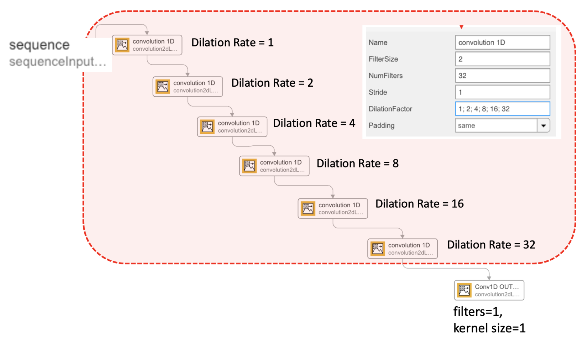
The second model depends on the idea of using convolutional layers consecutively, as seen in Figure 16. This architecture is known as the wavenet model, which was proposed by DeepMind in 2016 and has been widely used in text-to-speech tasks by Google. The wavenet methodology is inspired by combining two different techniques, respectively, wavelet and neural networks. Applying convolutional layers in the wavenet format is also very effective on time series forecasting tasks [48]. In the wavenet architecture, the dilation rate doubles at every layer. Dilated convolutions enable networks have very large receptive fields while preserving input resolution throughout the network as well as computational efficiency.
In the tested model, there were six consecutive CNN layers designed in the form of the wavenet architecture. The CNN layers had dilation rates of: 1, 2, 4, 8, 16, and 32, and each CNN layer had 32 filters of size two. The stride parameter was set to “one” to make one shift in each convolutional iteration. The padding parameter was set to “same” to make the output size equal to the input size. The last layer was also a convolutional layer that had a filter size of one, kernel size of one, and stride parameter set to one. As a result, the last layer produced a single output as the predicted value.
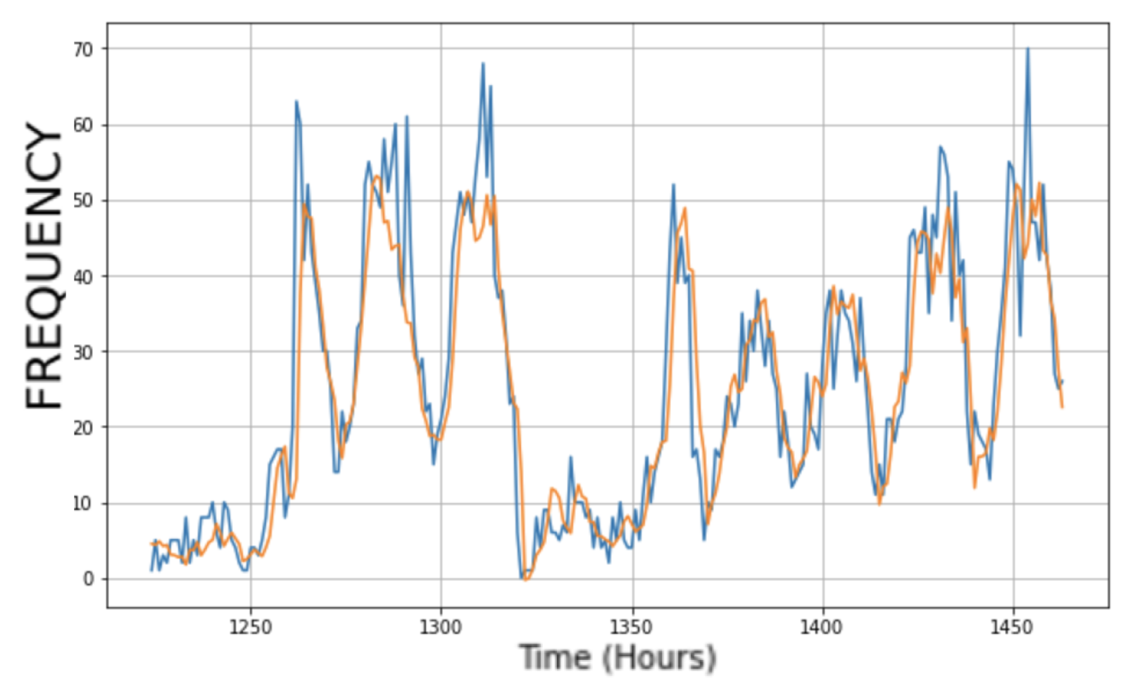
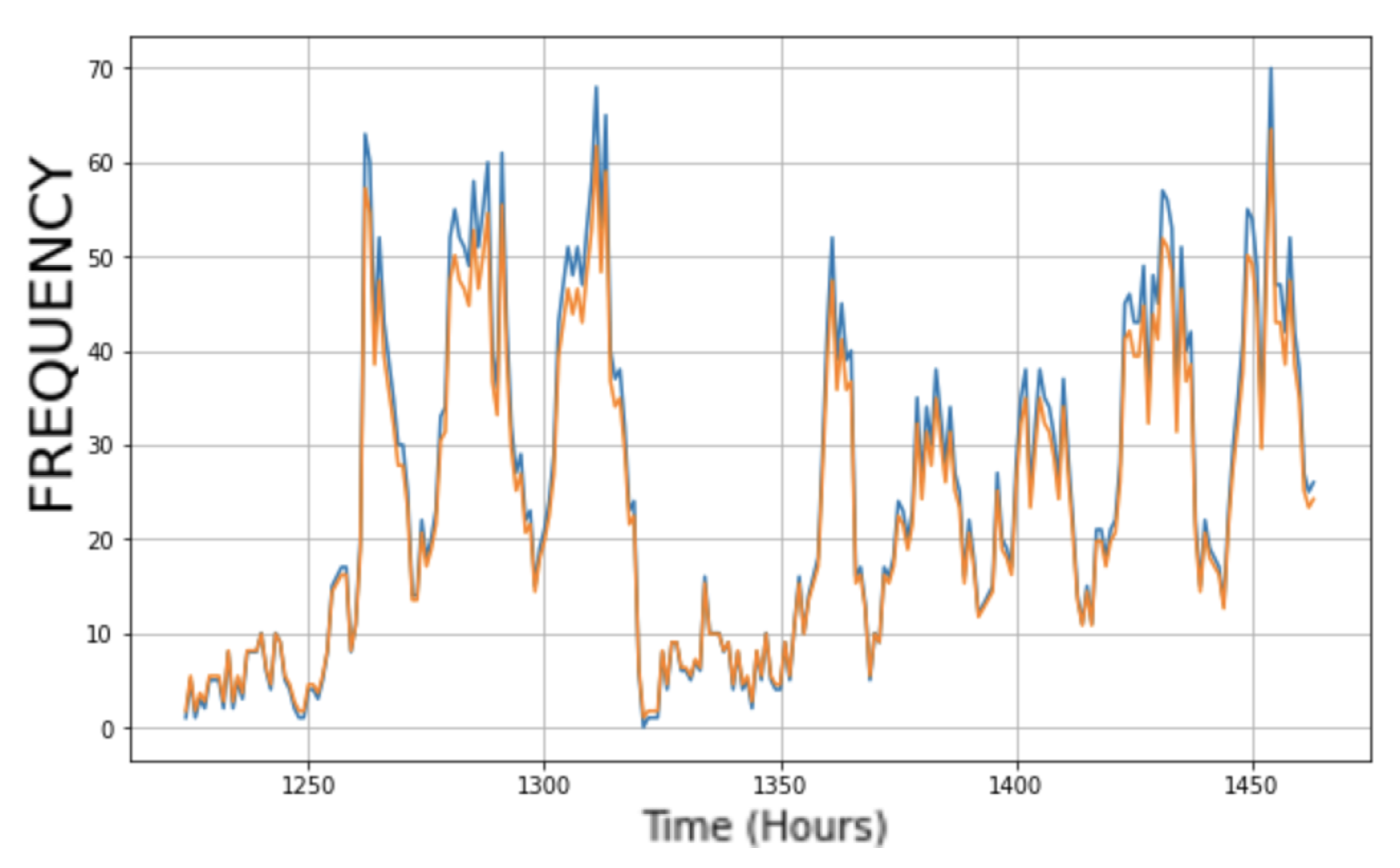
The forecasting performance of the full CNN model is presented in Figure 17, where the orange line is the predicted values, and the blue line is the real numbers. The full CNN model has a forecasting metric of 1.898 in terms of MAE. The full CNN model in the wavenet format performed better than all the other models. This result shows the strength of the wavenet architecture style.
6. Results and Conclusions
There are many well-known datasets, such as S&P 500, weather data, etc. We did not use these datasets because there have already been many experiments conducted on these data. Thus, we extracted a time series dataset from a real-world example. The time series used in this research was extracted from a software debugging web platform that projects the tendency of how frequently a specific tag is asked in blogs. Comparing the forecasting performances of some of the most used and famous models on a real-world time series gives clear insight into how accurate the models can perform.
We tested the most used models: MLP, RNN, LSTM, CNN, and the wavenet variant of CNN. They all have the same or similar complexity. All the models tested in this work were constructed in Google’s Colaboratory environment. The models were powered by TensorFlow version “2.8.2” and tensorflow.keras API version “2.8.0”, which are supported by Google for numerical computing, training, and running neural networks [49]. A list of the tested models and their basic specifications, such as the number of layers, the number of units in the layers, filters, etc., are presented in Table 1.
The prediction performance of the models is presented in Table 2. The metrics used to represent the forecasting performances were mean absolute error (MAE) and mean squared error (MSE). MAE computes the absolute values of the error, which are the differences between the predicted results and actual values. MSE computes the square of the errors. Consequently, MSE penalizes large errors more than MAE. If large errors are potentially more dangerous and cost much more than smaller errors, MSE is more beneficial than MAE.
According to the performance metrics, the fully convolutional layer model was the most successful in both MAE and MSE metrics. Especially, in terms of the MSE, which penalizes large errors more, the fully convolutional model achieved very successful forecasting performance. After the fully CNN Model, the most successful model was the LSTM model. Using the CNN layer as a pre-processing unit did not positively affect the forecasting performance of the LSTM model. Another important result is the success of the dense model. The dense model, consisting of two simple layers with ten units, also performed well when compared with its simplicity and compactness. The RNN models, both stateless and stateful versions, performed poorly. This is partly because RNN models suffer from transferring long-term information, which is known as the vanishing gradient problem.
The accuracy of time series prediction usually decreases as the forecast horizon increases. To measure the strength of the algorithms, we conducted more analyses using shorter window lengths. For example, on 5-day-long windows, the accuracy of the algorithms increased, and the model performances are compared in Table 3.
Another important metric for the tested models was the execution time and complexity. To enlighten this, the number of units, filters used in each layer, and the execution times are presented in Table 4. The metrics are acquired on a Python 3 Google Compute Engine (GPU mode) with 12.7 RAM.
To test the wavenet model’s resilience, we also conducted a preliminary test by using S&P 500 stock data between 16 December 2011 and 9 November 2017. According to this test, the wavenet model predicted the last 400 samples with a mean absolute value of 0.665. For future works, the wavenet model, which performed better than the memory models, can be compared by using a public dataset.
Author Contributions
Conceptualization, M.G. and F.U.; methodology, M.G. and F.U; software, M.G.; validation, M.G. and F.U.; writing—review and editing, M.G. and F.U. All authors have read and agreed to the published version of the manuscript.
Funding
This research received no external funding.
Data Availability Statement
The raw dataset, which was extracted from the StackOverflow website, and the time series extracted from this dataset are presented at https://github.com/mesuttguven/Trend-Prediction-on-Stack-Overflow-Dataset (accessed on 7 April 2023). The codes used in this paper are also presented on the GitHub page.
Conflicts of Interest
The authors declare no conflict of interest.
References
- Hu, Z.; Zhao, Y.; Khushi, M. A Survey of Forex and Stock Price Prediction Using Deep Learning. Appl. Syst. Innov. 2021, 4, 9. [Google Scholar] [CrossRef]
- Hyun, A.; Kyunghee, S.; Kwanghoon, P.K. Comparison of Missing Data Imputation Methods in Time Series Forecasting. Comput. Mater. Contin. 2022, 70, 423–431. [Google Scholar] [CrossRef]
- Wu, X.; Mattingly, S.; Mirjafari, S.; Huang, C.; Chawla, N.V. Personalized Imputation on Wearable Sensory Time Series via Knowledge Transfer. In Proceedings of the 29th ACM International Conference on Information & Knowledge Management, Virtual Event, Ireland, 19–23 October 2020; pp. 1625–1634. [Google Scholar] [CrossRef]
- Ramin Fadaei, F.; Orhan, E.; Emin, A. A DDoS attack detection and defense scheme using time-series analysis for SDN. J. Inf. Secur. Appl. 2020, 54, 102587. [Google Scholar] [CrossRef]
- Dwivedi, S.A.; Attry, A.; Parekh, D.; Singla, K. Analysis and forecasting of Time-Series data using S-ARIMA, CNN, and LSTM. In Proceedings of the 2021 International Conference on Computing, Communication, and Intelligent Systems (ICCCIS), Greater Noida, India, 19–20 February 2021; pp. 131–136. [Google Scholar]
- Bendong, Z.; Lu, H.; Chen, S.; Liu, J.; Wu, D. Convolutional neural networks for time series classification. J. Syst. Eng. Electron. 2017, 28, 162–169. [Google Scholar] [CrossRef]
- Han, Z.; Zhao, J.; Leung, H.; Ma, K.F.; Wang, W. A Review of Deep Learning Models for Time Series Prediction. IEEE Sens. J. 2021, 21, 7833–7848. [Google Scholar] [CrossRef]
- Omer Berat, S.; Mehmet Ugur, G.; Ahmet Murat, O. Financial time series forecasting with deep learning: A systematic literature review: 2005–2019. Appl. Soft Comput. J. 2020, 90, 106181. [Google Scholar] [CrossRef] [Green Version]
- Soheila Mehr, M.; Mohammad Reza, K. An analytical review for event prediction system on time series. In Proceedings of the 2nd International Conference on Pattern Recognition and Image Analysis, Rasht, Iran, 11–12 March 2015. [Google Scholar]
- Kim, K.J. Financial time series forecasting using support vector machines. Neurocomputing 2003, 55, 307–319. [Google Scholar] [CrossRef]
- Lai, R.K.; Fan, C.Y.; Huang, W.H.; Chang, P.C. Evolving and clustering fuzzy decision tree for financial time series data forecasting. Expert Syst. Appl. 2009, 4, 3761–3773. [Google Scholar] [CrossRef]
- Shen, L.; Loh, H.T. Applying rough sets to market timing decisions. Decis.Support Syst. 2004, 37, 583–597. [Google Scholar] [CrossRef]
- Patel, J.; Shah, S.; Thakkar, P.; Kotecha, K. Predicting stock market index using fusion of machine learning techniques. Expert Syst. Appl. 2015, 42, 2162–2172. [Google Scholar] [CrossRef]
- Zhang, X.; Shi, J.; Wang, D.; Fang, B. Exploiting investors social network for stock prediction in China’s market. J. Comput. Sci. 2018, 28, 294–303. [Google Scholar] [CrossRef] [Green Version]
- Kumar, I.; Dogra, K.; Utreja, C.; Yadav, P. A Comparative Study of Supervised Machine Learning Algorithms for Stock Market Trend Prediction. In Proceedings of the 2018 Second International Conference on Inventive Communication and Computational Technologies (ICICCT), Coimbatore, India, 20–21 April 2018; pp. 1003–1007. [Google Scholar] [CrossRef]
- Zhou, F.; Zhou, H.m.; Yang, Z.; Yang, L. EMD2FNN: A strategy combining empirical mode decomposition and factorization machine based neural network for stock market trend prediction. Expert Syst. Appl. 2019, 115, 136–151. [Google Scholar] [CrossRef]
- Chen, K.; Zhou, Y.; Dai, F. A LSTM-based method for stock returns prediction: A case study of China stock market. In Proceedings of the 2015 IEEE International Conference on Big Data, Santa Clara, CA, USA, 29 October–1 November 2015; pp. 2823–2824. [Google Scholar] [CrossRef]
- Persio, L.D.; Honchar, O. Recurrent neural networks approach to the financial forecast of Google assets. Int. J. Math. Comput. Simul. 2017, 11, 1–7. [Google Scholar]
- Blem, M.; Cristaudo, C.; Moodley, D. Deep Neural Networks For Online Trend Prediction. In Proceedings of the 2022 25th International Conference on Information Fusion (FUSION), Linköping, Sweden, 4–7 July 2022; pp. 1–8. [Google Scholar] [CrossRef]
- Chandola, D.; Mehta, A.; Singh, S.; Tikkiwal, V.A.; Agrawal, H. Forecasting Directional Movement of Stock Prices using Deep Learning. Ann. Data Sci. 2022. [Google Scholar] [CrossRef]
- Kittisak, P.; Peerapon, V. Stock Trend Prediction Using Deep Learning Approach on Technical Indicator and Industrial Specific Information. Information 2021, 12, 250. [Google Scholar] [CrossRef]
- Liu, S.; Zhang, C.; Ma, J. CNN LSTM Neural network model for quantitative strategy analysis in stock markets. In Neural Information Processing; Springer International Publishing: Berlin, Germany, 2017; pp. 198–206. [Google Scholar] [CrossRef]
- Batres-Estrada, B. Deep Learning for Multivariate Financial Time Series. Master’s Thesis, KTH, Mathematical Statistics , Stockholm, Sweden, 2015. [Google Scholar]
- Wang, K.; Li, K.; Zhou, L.; Hu, Y.; Cheng, Z.; Liu, J.; Cen, C. Multiple convolutional neural networks for multivariate time series prediction. Neurocomputing 2019, 360, 107–119. [Google Scholar] [CrossRef]
- Lian, L.; Tian, Z. A novel multivariate time series combination prediction model. Commun. Stat.-Theory Methods 2022, 1–32. [Google Scholar] [CrossRef]
- Ong, Y.J.; Qiao, M.; Jadav, D. Temporal Tensor Transformation Network for Multivariate Time Series Prediction. In Proceedings of the 2020 IEEE International Conference on Big Data (Big Data), Atlanta, GA, USA, 10–13 December 2020. [Google Scholar] [CrossRef]
- Hornik, K. Approximation capabilities of multilayer feed forward networks. Neural Netw. 1991, 4, 251–257. [Google Scholar] [CrossRef]
- Robert, R. Can periodic perceptrons replace multi-layer perceptrons? Pattern Recognit. Lett. 2000, 21, 1019–1025. [Google Scholar]
- Chatterjee, A.; Saha, J.; Mukherjee, J. Clustering with multi-layered perceptron. Pattern Recognit. Lett. 2022, 155, 92–99. [Google Scholar] [CrossRef]
- Schuster, M.; Paliwal, K.K. Bidirectional Recurrent Neural Networks. IEEE Trans. Signal Process. 1997, 45, 2673–2681. [Google Scholar] [CrossRef] [Green Version]
- Moharm, K.; Eltahan, M.; Elsaadany, E. Wind Speed Forecast using LSTM and Bi-LSTM Algorithms over Gabal El-Zayt Wind Farm. In Proceedings of the 2020 International Conference on Smart Grids and Energy Systems (SGES), Perth, Australia, 23–26 November 2020. [Google Scholar] [CrossRef]
- Roy, S.S.; Awad, A.I.; Amare, L.A.; Erkihun, M.T.; Anas, M. Multimodel Phishing URL Detection Using LSTM, Bidirectional LSTM, and GRU Models. Future Internet 2022, 14, 340. [Google Scholar] [CrossRef]
- Sarıgul, M.; Ozyildirim, B.M.; Avci, M. Differential convolutional neural network. Neural Netw. 2019, 116, 279–287. [Google Scholar] [CrossRef]
- Qu, Y.; Zhang, N.; Meng, Y.; Qin, Z.; Lu, Q.; Liu, X. ECG Heartbeat Classification Detection Based on WaveNet-LSTM. In Proceedings of the 2020 IEEE the 4th International Conference on Frontiers of Sensors Technologies, Shanghai, China, 6–9 November 2020. [Google Scholar] [CrossRef]
- Rathore, N.; Rathore, P.; Basak, A.; Nistala, S.H.; Runkana, V. Multi Scale Graph Wavenet for Wind Speed Forecasting. In Proceedings of the 2021 IEEE International Conference on Big Data (Big Data), Orlando, FL, USA, 15–18 December 2021. [Google Scholar] [CrossRef]
- LeCun, Y.; Bengio, Y.; Hinton, G. Deep learning. Nature 2015, 521, 436–444. [Google Scholar] [CrossRef] [PubMed]
- Jurgen, S. Deep learning in neural networks: An overview. Neural Netw. 2015, 61, 85–117. [Google Scholar] [CrossRef] [Green Version]
- Li, H.; Li, J.; Guan, X.; Liang, B.; Lai, Y.; Luo, X. Research on overfitting of deep learning. In Proceedings of the 15th International Conference on Computational Intelligence and Security (CIS), Macao, China, 13–19 December 2019; pp. 78–81. [Google Scholar] [CrossRef]
- Kai, W.; Jufeng, Y.; Guangshun, S.; Qingren, W. An expanded training set based validation method to avoid overfitting for neural network classifier. In Proceedings of the Fourth International Conference on Natural Computation, Jinan, China, 18–20 October 2008; pp. 83–87. [Google Scholar] [CrossRef]
- José, F.T.; Dalil, H.; Abderrazak, S.; Martínez-Álvarez, F.; Alicia, T. Deep learning for time series forecasting: A survey. Big Data 2021, 9, 3–21. [Google Scholar] [CrossRef]
- Rumelhart, D.E.; Hinton, G.E.; Williams, R.J. Learning internal representations by error propagation. In Parallel Distributed Processing: Explorations in Microstructure of Cognition; California Univ San Diego La Jolla Inst for Cognitive Science: San Diego, CA, USA, 1985. [Google Scholar]
- Alex, S. Fundamentals of recurrent neural network (RNN) and long short-term memory (LSTM) network. Phys. D Nonlinear Phenom. 2020, 404, 132306. [Google Scholar] [CrossRef] [Green Version]
- Sundermeyer, M.; Schlüter, R.; Ney, H. LSTM neural networks for language modeling. In Proceedings of the Thirteenth Annual Conference of the International Speech Communication Association, Portland, OR, USA, 9–13 September 2012; pp. 9–13. [Google Scholar]
- Zewen, L.; Fan, L.; Wenjie, Y.; Shouheng, P.; Jun, Z. A survey of convolutional neural networks: Analysis, applications, and prospects. IEEE Trans. Neural Netw. Learn. Syst. 2021, 33, 6999–7019. [Google Scholar] [CrossRef]
- Neena, A.; Geetha, M. A review on deep convolutional neural networks. In Proceedings of the 2017 International Conference on Communication and Signal Processing, Tamilnadu, India, 6–8 April 2017; pp. 0588–0592. [Google Scholar]
- Jiuxiang, G.; Wang, Z.; Kuen, J.; Ma, L.; Shahroudy, A.; Shuai, B.; Liu, T. Recent advances in convolutional neural networks. Pattern Recognit. 2018, 77, 354–377. [Google Scholar] [CrossRef] [Green Version]
- Ayodeji, A.; Wang, Z.; Wang, W.; Qin, W.; Yang, C.; Xu, S.; Liu, X. Causal augmented ConvNet: A temporal memory dilated convolution model for long-sequence time series prediction. Isa Trans. 2022, 123, 200–217. [Google Scholar] [CrossRef]
- Jonathan, B.; Philippe, G.; Roch, L. A literature review of wavenet: Theory, application, and optimization. In Audio Engineering Society Convention 146; Audio Engineering Society: New York, NY, USA, 2019. [Google Scholar]
- Geron, A. Hands-On Machine Learning with Scikit-Learn and TensorFlow: Concepts, Tools, and Techniques to Build Intelligent Systems; O’Reilly Media, Inc.: Sebastopol, CA, USA, 2019. [Google Scholar]
Figure 1.
Dataset.

Figure 2.
Occurrences Based on Tags Groups.

Figure 3.
Time series of the asked questions with the tag value of python.

Figure 4.
Flowchart of the methodology.

Figure 5.
Dense model representation.

Figure 6.
Loss value versus learning rate.

Figure 7.
Forecasting performance of the dense model.

Figure 8.
RNN model structure.

Figure 9.
Forecasting performance of the stateless RNN model.

Figure 10.
Forecasting performance of the stateful RNN model.

Figure 11.
LSTM model representation.

Figure 12.
LSTM architecture.

Figure 13.
Forecasting performance of the LSTM model.

Figure 14.
Representation of the hybrid model with CNN and LSTM layers.

Figure 15.
Forecasting performance of the hybrid model.

Figure 16.
Representation of the full CNN model.

Figure 17.
Forecasting performance of the fully CNN model.


Table 1.
Tested models and properties.
| MODEL | LAYERS | FUNCTIONS |
|---|---|---|
| Dense | 3 Dense | ReLu, Linear |
| Stateless RNN | 2 RNN, 1 Dense | tanh, Linear |
| Stateful RNN | 2 RNN, 1 Dense | tanh, Linear |
| LSTM | 2 LSTM, 1 Dense | tanh-Sigmoid, Linear |
| CNN Hybrid | 1 CNN, 2 LSTM, 1 Dense | ReLu, tanh, Linear |
| Fully CNN | 6 CNN, 1 CNN | ReLu |
Table 2.
Model performance comparison.
| MODEL | MAE 1 | MSE 2 |
|---|---|---|
| Dense | 5.5728846 | 61.942547 |
| Stateless RNN | 6.6797476 | 82.98067 |
| Stateful RNN | 7.0399313 | 96.302475 |
| LSTM | 5.3750377 | 59.87254 |
| CNN Hybrid | 5.3894196 | 62.422806 |
| Fully CNN | 1.8986198 | 6.2615194 |
MAE 1: mean absolute error; MSE 2: mean squared error.
Table 3.
Model performance comparison on 5-day-long windows.
| MODEL | MAE-1 1 | MAE-2 2 |
|---|---|---|
| Dense | 5.5728846 | 5.9691405 |
| Stateless RNN | 6.6797476 | 6.0903750 |
| Stateful RNN | 7.0399313 | 6.1267543 |
| LSTM | 5.3750377 | 5.3358135 |
| CNN Hybrid | 5.3894196 | 5.9622736 |
| Fully CNN | 1.8986198 | 1.2275864 |
MAE 1: mean absolute error for 10-day-long predictions; MSE 2: mean absolute error for 5-day-long predictions.
Table 4.
Model complexity and execution time.
| MODEL | COMPLEXITY | TIME (Second Per Epoch) |
|---|---|---|
| Dense | 3 layers; 10, 10, 1 units | 0.431 |
| Stateless RNN | 3 layers; 100, 100, 1 units | 1.272 |
| Stateful RNN | 3 layers; 100, 100, 1 units | 0.575 |
| LSTM | 3 layers; 100, 100, 1 units | 1.038 |
| CNN Hybrid | 4 layers; 32, 32, 32, 1 filters | 0.919 |
| Fully CNN | 7 layers; 32, 32, 32, 32, 1 filters | 0.722 |
Disclaimer/Publisher’s Note: The statements, opinions and data contained in all publications are solely those of the individual author(s) and contributor(s) and not of MDPI and/or the editor(s). MDPI and/or the editor(s) disclaim responsibility for any injury to people or property resulting from any ideas, methods, instructions or products referred to in the content. |
© 2023 by the authors. Licensee MDPI, Basel, Switzerland. This article is an open access article distributed under the terms and conditions of the Creative Commons Attribution (CC BY) license (https://creativecommons.org/licenses/by/4.0/).
Share and Cite
MDPI and ACS Style
Guven, M.; Uysal, F. Time Series Forecasting Performance of the Novel Deep Learning Algorithms on Stack Overflow Website Data. Appl. Sci. 2023, 13, 4781. https://doi.org/10.3390/app13084781
AMA Style
Guven M, Uysal F. Time Series Forecasting Performance of the Novel Deep Learning Algorithms on Stack Overflow Website Data. Applied Sciences. 2023; 13(8):4781. https://doi.org/10.3390/app13084781
Chicago/Turabian StyleGuven, Mesut, and Fatih Uysal. 2023. "Time Series Forecasting Performance of the Novel Deep Learning Algorithms on Stack Overflow Website Data" Applied Sciences 13, no. 8: 4781. https://doi.org/10.3390/app13084781
Note that from the first issue of 2016, this journal uses article numbers instead of page numbers. See further details here.