On Selecting, Ranking, and Quantifying Features for Building a Liver CT Diagnosis Aiding Computational Intelligence Method

Featured Application

The selected attributes and their ranking and weights can be used in decision support algorithms in computer aided diagnosis.

Abstract

The liver is one of the most common locations for incidental findings during abdominal CT scans. There are multiple types of disease that can arise within the liver and many of them are nodular. The ultimate goal of our research is to develop an expert knowledge-based system using fuzzy signatures, to support decisions during diagnosis of the most frequent of these nodular lesions. Since the literature contains limited information about the graphical properties of CT images that must be taken into consideration and their relationship to one another, in this paper we focused on selecting and ranking the input parameters using expert knowledge and determining their importance. Six visual attributes of lesions (size, shape, density, homogeneity contour, and other features) were selected based on textbooks of radiology and expert opinion. The importance of these attributes was ranked by radiologist experts using questionnaires and a pairwise comparison technique. The most important feature was found to be the density of the lesion on the various CT phases, and the least important was the size, the order of the other attributes was other features, contour, homogeneity, and shape, with a Kendall concordance coefficient of 0.612. Weights for the attributes, to be used in the future fuzzy signatures, were also determined. As a last step, several statistical parameter-based quantities were generated to represent the above abstract attributes and evaluated by comparing them to expert opinions.

1. Introduction

Medical decision support systems are a broadly researched area at present. Many research groups are working on algorithms for better segmentation, recognition, and characterization. The purpose of artificial intelligence and computer-aided diagnosis (CAD) is not to substitute doctors but to help them and decrease the possibility of misdiagnosis.

In the past decades, outstandingly successful neural network (NN) based applications have emerged in pattern recognition, including computer-aided medical diagnostic procedures. Since NNs perform particularly well when analyzing images, more and more NN-based approaches are being proposed for disease recognition in CT images. NNs are taught by training samples. In an ideal case, researchers have access to large numbers of medical cases. Miah suggested a NN-based model for lung cancer detection. His NN was trained with 300 samples [1]. Skourt used 1018 samples of the LIDIC-IDRI public database for creating his lung CT image segmentation model [2], Aghamohammadi used the samples of 1000 patients for CT tumor and liver segmentation [3], Hermann used 53,000 photographs for melanoma classification [4], while Shu had 994 pictures to create his adaptive segmentation model for liver CT images [5] (we note that, in this last case, Shu’s 994 samples were derived from only 24 patients, so even though they were obviously taken from different layers, they cannot necessarily be considered different samples). In the listed cases, each of which used NNs, the number of the samples ranged from a few hundred to several thousand. Although the literature does not specify an exact value for the minimum number of teaching samples, the more samples, the higher the accuracy of the NN. Lange and Manner experimented with training sets of different sizes and showed that there is a critical size of the training set, which is dependent on the number of weights used in the NN [6]. A more detailed interpretation of this is outside the scope of this paper, but it can be stated that NN-based medical applications must not be created using only a few tens of images.

If there are not enough samples (note that, due to the General Data Protection Regulation of the European Parliament, few samples are available for medical studies), a neural network with sufficient accuracy cannot be created. There are ways to circumvent this problem, such as using data augmentation, transfer learning, or GAN networks, which in the medical community still imply the question of whether these artificial intelligence methods can provide sufficiently reliable methods that can be used in CAD.

Instead, an expert system based on medical knowledge can be constructed, which can be made more accurate with the data of certain available samples. Fuzzy systems [7], or fuzzy signatures are especially suitable for creating such solutions. Such systems perform surprisingly well in fields with data that can be collected from a lot of work, e.g., in civil engineering, where earthquake resistance [8] or structural condition is assessed [9].

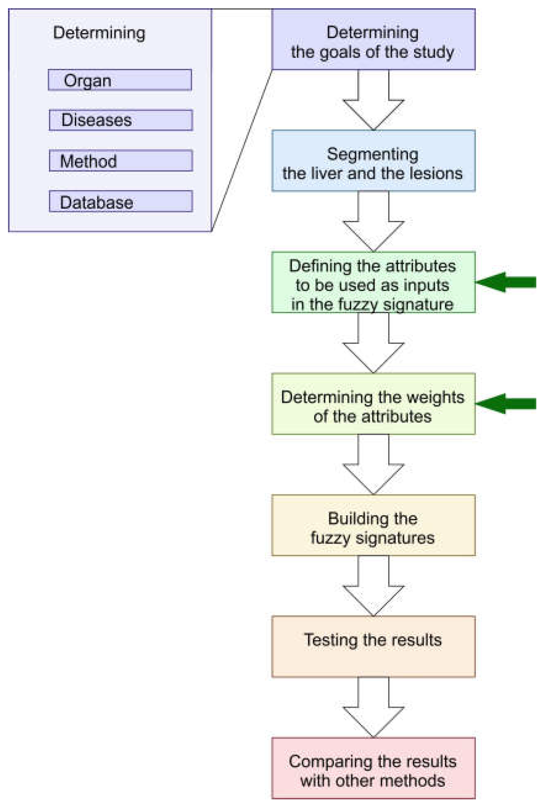
Fuzzy signatures can implement expert knowledge in a very plausible way, and using fuzzy signatures is very advantageous if not all the possible inputs are always present, and it can handle missing data in a very flexible way. This is the reason that our research focused on fuzzy signature-based methods [10,11]. The flowchart for building our method can be seen in Figure 1, with the steps in the paper marked by green arrows.

In our research, we selected the liver as the organ, and CT as the scanning method due to of the following reasons.

One of the key organs during any kind of abdominal imaging is the liver, and incidental findings are very common. An incidental finding means any lesion that causes no symptoms and whose exploration was not the purpose of the examination. They include many benign lesions, but many malignant tumors and metastases are also found by screening “healthy” people or patients with subtle and general symptoms. Metastatic liver disease is many times more common than primary liver tumors. Finding liver metastasis means that the disease is advanced and possibly affects the whole body, so the cure needs to be changed to a more aggressive one. The reason why the liver is a common site for the remote spreading of tumors is its dual blood supply. Small lesions (<15 mm) of the liver are frequently detected by routine ultrasound (US) or computer tomography (CT) studies. About 30% of such lesions are malignant in the whole population; however, in the case of patients with previously known other malignancies, this ratio is 50% [12].

Targeted detection of liver metastases in patients with known neoplasms is primarily done by CT examination. These are so-called screening examinations, which can be followed by some other, more specific type, such as hepatocyte-specific MRI or even biopsies. A baseline CT is performed in almost every cancer case for reference. After treatment or after certain stage points, a control CT is performed to follow the recent changes. This is very important, but with the naked eye it is not always possible to detect subtle signs of metastases in CT and to differentiate them from benign lesions which can imitate malignancies when they are small.

In the recent literature, the majority of the methods focused on the most frequent diseases in the liver, which is probably the reason for the low number of images of the less common lesions that could be used for training and testing. In the available studies, many of the methods can only distinguish malignant and benign lesions, without further differentiation [13,14,15,16]. Many of the authors carried out research on a more detailed classification. There were experiments on differentiating between two or maybe three lesions that are significantly different in appearance [17,18,19]. However, there have been few researchers who could classify these diseases at the same time and not just distinguish between a few categories [20].

Many research groups studied only one phase of the CT protocol, either the non-enhanced [15,20,21,22,23] or the portal [24,25,26] phase, which is usually not sufficient for a proper decision, according to general medical opinion. However, there were a few teams who used all the available CT phases [27,28,29].

For this reason, we started to develop a method that can later be used as a basis of an overall intelligent computer-aided diagnosis algorithm. As well-prepared medical images are expensive to prepare and rare in the case of the liver, especially such images where the different phases of the CT scans can be found for the same lesion, we decided to build an expert system instead of a self-learning one.

The first step of building such an expert system is to select the attributes of the images that are important in the decision making and also to determine to what extent these features are important and how to quantify them. This paper summarizes our methodology and findings for selecting the input attributes for a fuzzy signature-based decision support system and for quantifying them.

This paper consists of the following parts. After a brief introduction, Section 2 (Materials and Methods) contains a paragraph about computed tomography, as well as the importance of the various phases of an abdominal CT protocol. The attributes used by medical experts are defined in Section 2.3. After a short summary of the image-related methods used in the study in Section 2.5, the statistical methods used during the ranking of the selected attributes are listed in Section 2.6. Section 3 (Results) consists of two parts. Section 3.1 describes the ranking process in detail, while Section 3.2 gives the numerical quantities that were suggested for representing the abstract medical attributes, size, shape, density, homogeneity, and contour. In Section 4, a short discussion of the results can be found. The article contains two appendices, the first gives a short summary about the biology of the liver, which helps in understanding the characteristics of the lesions in the images of the different phases. The second part shows questions from the questionnaire we used for studying the expert opinions.

2. Materials and Methods

2.1. About the CT Images

Computed tomography (CT) is a widely used method for liver imaging [30]. The basic idea of CT is that the body is scanned by X-rays from multiple angles, and from these images the attenuation quotient for every pixel is computed. From these data, a 3D-map of the examined voxel can be built. Inside the voxel, the tissues can be differentiated by their different attenuation quotient, which is normalized to the attenuation of water. This normalized scale is the Hounsfield scale, and its units are Hounsfield units (HU) [31]; in which, 0 HU is the attenuation (density) of the water and −1000 HU is the density of the air. Soft tissues such as liver and tumor tissue are around 20–60 HU on non-enhanced images, depending on their fat content. The computer gives every Hounsfield unit a shade of the color gray. It can be seen that, if we used the whole scale of the HU levels, the gray shades of the soft tissues would be indistinguishable from each other [32]. Therefore, a special medical image format called DICOM (digital imaging and communications in medicine) is used for medical images [33]. This has the capacity to handle a large density range and has the capability to tailor it to the needs of the operator. Using the DICOM file format, a range can be set, in which the computer divides the visible 30–60 shades of gray, to give a better contrast. This is called windowing. This is why it is important to use original DICOM files and not conventional image formats, because with the latter a huge amount of information could be lost. The DICOM file format contains not only the image data, but the patient personal data are also embedded. These are strictly protected by European and American law (GDPR in EU [34], HIPAA in USA [35]). To remove them, the first step of data gathering should be anonymization. This can be a rather time-consuming process with large amounts of data. The strict EU and USA laws regarding patient rights are the main reason why no huge databases of medical data are accessible. Another reason could be that many of the diseases are rare or, especially in benign lesions, do not need further imaging after they are discovered. In these scenarios, the large database that a proper and accurate deep learning system would demand is not collectable. Our solution to this problem is that we started to develop a system which can work with rather small amounts of medical data. We want to use expert knowledge processed on the basis of fuzzy signatures to complement the image processing systems, for a better and medically acceptable result.

2.2. CT Medical Protocol in the Case of the Liver and Abdomen

The main aim of a diagnostic algorithm is to exclude or consider the malignancy of a liver lesion. For this purpose, different imaging and laboratory tests are used and all the information are synthesized. In every case, this assessment is made by a team of qualified doctors, which consumes a lot of working hours and money, and of course the process has the possibility of errors in many forms. With a computer-assisted system, the errors could be minimized [36,37].

For distinguishing different tissues inside the parenchymal organs such as the liver, contrast material is needed. Positive contrast material changes the attenuation of the tissues, as they contain substances with high atomic numbers, which increases the attenuation of the X-rays inside the tissue. This can give a hint or show directly the altered vascularization (blood supply) of a lesion compared to normal tissue.

After giving iodinated contrast material, a CT examination can be performed at different time points and different results will come back, according to the location of the contrast material inside the vascular system. Different institutions sometimes use different phases for routine examinations (protocols), different machines, and slightly different timings. These timing data and contrast material data are embedded in DICOM files.

The native or non-enhanced phase (NECT) is taken before giving the intravenous contrast material. This is usually for detecting calcifications and bleeding, and serves as a reference series for contrast-enhanced phases. The most important phases in connection with liver nodular diseases are the arterial phase (20–40 s after injecting the contrast material) and the portal phase (50–90 s). In these phases, alterations of the vasculature inside non-normal tissues of the liver can be detected. Another useful phase is the so-called delayed phase (5–15 min), where poorly vascularized tissues are enhanced and can give additional information, aiding the diagnosis. Unfortunately, the use and timing of these phases are different from institute to institute, as is the type of CT machine. These differences can make unsupervised machine learning difficult, which fact also led us to build a conventional expert-based diagnostic system [32].

2.3. Characteristics of the Liver Nodules to Be Quantified in a CT: The Main Features

During the diagnostic process, the radiologist searches for features such as an abnormal shape, density, or inhomogeneity. From these features, the doctor can define the lesion’s characteristics and more or less classify the lesion as benign or malignant. The main characteristics of the lesion are the shape, density, enhancement, morphology, size, and multiplicity.

In this section, the main imaging features of liver nodules are introduced. Our purpose is to show the most important properties that are examined during the segmentation and processing steps. This list is not a full one and does not show every possible lesion type in the liver (not even all forms of the presented ones), only the most frequent and important. It focuses only on the CT features of the nodules from an image processing point of view. Moreover, only normal or slightly fatty liver is considered as the background for the lesions. These features were selected by synthetizing data from different textbooks [38,39,40], where they are collected from the radiologists’ point of view.

2.3.1. Shape

Most of the circumscribed lesions of the liver, the so-called focal nodules, are roundish or ellipsoid, although perfectly regular shapes are occasionally present. Usually, there are some lobulations or imperfections. Simple cysts are the most round, as the inner fluid expands into the normal liver centrically. The other nodules with tissue (non-fluid) structure rarely have a strictly regular shape.

2.3.2. Contour

An ill-defined contour suggests aggressive, fast-growing disease; however, many hepatic cell carcinomas and metastases have well-defined borders. A well-defined border can be seen when there is tissue death (necrosis) inside the lesion, or when there is a highly vascularized viable tumor tissue at the borders; this causes hyperenhancement in contrast-enhanced images, which has a well-observable tissue contrast with the normal liver. Small and well-defined neoplasms can also have smooth contours. Lobulation can be a morphological feature, which is however nonspecific: benign and malignant lesions can also be lobulated, e.g., both benign hemangiomas and the malignant fibrolamellar carcinoma can be lobulated.

2.3.3. Density

Density is examined in all four phases as it changes with time. As blood flows through the vessels, the tissue changes its capability for X-ray absorption, so the attenuation quotient differs, and this is reflected as a different number of Hounsfield units. In non-enhanced scans, most of the lesions are iso- or hypodense. If the lesion is hyperdense in the non-enhanced phase, this means that it contains blood (50–70 HU) or calcification (over 120 HU). In contrast-enhanced phase, the blood supply of the lesion is examined. Malignant primary lesions have a massive arterial supply, which makes them hyperdense in arterial phase images. Hyperdensity is not necessarily homogeneous; usually small lesions are homogenous, and larger ones have more or less heterogeneous enhancement. Washout is a sign indicating mostly arterial blood flow, which is typical for a malignant lesion. In CT images, such nodules show a bright enhancement in the arterial phase and a relative hypovascularity in comparison with the normal tissues the in portal and late phases. Benign lesions such as FNH and adenoma show bright arterial enhancement with an iso- or slightly hyperdense appearance on the portal and delayed phase. Lesions which are isodense in the portal phase are most probably non-malignant.

2.3.4. Homogeneity

A lesion is homogenous when it contains similar tissues. Clustered distribution of cells, internal hemorrhage, necrosis, calcification, and scarring cause inhomogeneity. Larger lesions can develop necrosis. Some lesions, such as adenoma or HCC can bleed inside. Scarring is usually a characteristic feature and occurs in FNH and some types of liver cancer.

2.3.5. Size

Radiologists consider size to be an important factor; however, it does not have a real predictive value. It is nonspecific, but can provide additional information during the diagnosis-making process. In malignant diseases, a larger size indicates a more advanced stage of the disease that, therefore, usually requires a different management; however, a benign lesion can grow large without any signs or importance.

2.3.6. Other Features

As we have seen, contour, density, enhancement, and even the shape in some cases can vary with time and phase. This is why we suggest examining liver lesions at all approachable phases of time. Additional features, such as a capsule, central scar, calcification, enhancement in delayed phases, etc., are more or less specific for diseases and are not common feature to be evaluated individually. However, they are important findings if they are present.

2.4. Important Features of Liver Lesions and How to Recognize Them

We selected for our research the most frequent focal liver lesions. Their most important characteristics in CT images are summarized in

Table 1. The properties of the focal nodular lesions.

Focal Liver Lesion	Characteristic CT Features
Cyst	near water-density fluid content no enhancement round solitary or multiple
Hemangioma	contrast enhancement follows the blood pool nodular peripheral enhancement in the arterial phase graduate filling-in from the periphery in the later phases prolonged enhancement in delayed phase can be observed
Focal Nodular Hyperplasia (FNH)	often beneath the liver surface well-demarcated borders can be lobulated usually solitaire characteristic low-density central scar (delayed enhancement) spoke-wheel enhancement pattern (most convenient is early arterial phase) isodense in portal and delayed phase
Hepatic Adenoma	sharp contour can be inhomogeneous (especially if large)—bleeding, necrosis, calcification arterial enhancement, can be undistinguishable later phases
Hepatocellular Carcinoma (HCC)	different tissue types can show different appearances avid enhancement in the arterial phase washout in portal and delayed phase rim-enhancement in the delayed phase
Metastases	variable appearance marked washout in portal and delayed phase can be heterogeneous (especially if larger)

. For more detail, as well as a very brief summary of the biological background, see Appendix A.1.1–A.1.6.

2.5. Image Processing Tasks Related to Finding and Characterizing Liver Nodular Lesions

The liver is a rather interesting organ from an image processing point of view. As is evident from the previous sections, the liver is very diverse, and the lesions diagnosed with computational aid are also of multiple types and can manifest in various shapes, sizes, and densities, with different density distributions, both spatially and during the various phases of the measurement. There are two basic image processing tasks regarding the liver in medical diagnosis aiding applications.

2.5.1. Segmentation

The task of segmentation in general image processing is to define different (mostly non-overlapping) domains among the pixels or voxels that correspond to various organs, beside the liver, veins, gallbladder, or the lesions themselves. This segmentation task can be two- or three-dimensional, or it can even include different phases of the CT data. On the contrary to the medical usage, segmentation from an image processing point of view mostly does not include the identification of the actual, medical liver segments, so this nomenclature needs to be clarified between the two communities.

2.5.2. Classification

The task is to give a tag or class to the pixels/voxels or the already segmented groups of pixels or voxels. This classification can mean identifying an organ, a region, an intensity domain, or even the type of the lesion.

2.5.3. Guidelines for CT Image Processing for Decision Support Purposes

During our research, we faced several problems regarding the cooperation of people with medical and engineering backgrounds. This is the reason why a short summary of our rules for cooperation are given in the following points.

• Biology means diversity. Liver is an especially diverse an organ, it can have many shapes, sizes, and density ranges. The lesions in the liver are diverse as well.
• The goal should be to build a method that is good enough to help medical experts, not replacing them.
• If a disease is found, it does not mean that there cannot be another, different or maybe the same type.
• There are lots of types of lesions that can be found in a liver CT. Some of them are extremely rare, yet very dangerous. It is very difficult to build a sufficiently large training set for all the possible outputs of a purely deep learning liver diagnosis program.
• There is a possibility to suggest other diagnostic methods, if the data from the CT is not sufficient to give reliable results. It is possible to have an exit code “order another type of diagnostic procedure” (even biopsy) for a medical image classification program.
• It is necessary to clarify the goal of the classification and the mathematical measure in which the hit rate should be high. It is necessary to describe the usual measures of hit rates to medical experts and to discuss if they are a sufficient or necessary measure for them. It might take more rounds to clarify the goals.
• A medical method should be tested for a long time (several years) before validation. It is necessary to help the medical experts understand how the image processing or classification method works and what are the critical points for testing.

2.5.4. Image Preprocessing in this Study

As the liver itself is rather noisy in CT images, many of the lesions have a very blurry contour; moreover, some lesions have very sharp edges inside them and a blurry outer contour at the same time. Segmentation of all possible lesion types is a very challenging task. Lesion segmentation can be done manually, semi-automatically, or automatically. Each method has its advantages and disadvantages, which are beyond the scope of this article. A wide-ranged review is given in the paper of Nayantara et al. [41]. Previously, we tried several methods, including clustering and active contours with initial contours based on expert knowledge, but none of these methods could give contours that would be fully acceptable for medical experts. In our recent research, we focused on classification of lesions that are already segmented and have at least arterial and portal phase data at approximately the same position.

In addition, our goal was to determine which are the most important characteristics of these lesions and how to quantify them in a manner that it is acceptable and understandable, both for medical experts and engineers, as well as computer scientists.

For this purpose, the first step is to collect the attributes that are used by the medical community and rank them according to importance using the medical experts’ opinion. The next step (which is beyond the scope of this paper) is to implement these attributes in a computationally understandable way.

2.6. Ranking of Features Based on Expert Opinions

In the multi-attribute decision making models of complex systems, the goal is to order the possible choices based on an evaluation of the possibilities. An attribute is such a property that is considered in the evaluation process, not by itself, but as a part of the ordering.

During the selection of features, considering all possible aspects of the system, it is necessary to determine those attributes that are dominant. It is not possible to use such attributes that exclude each other completely or cannot be represented by numbers. Moreover, the attributes should be independent of each other.

During our study, we followed the steps listed below.

2.6.1. Selecting the Set of Attributes

The attributes can be selected based on expert knowledge.

Let us denote the number of the attributes by $n$.

2.6.2. Generating a Pairwise Comparison Questionnaire

The $n$ attributes should be paired in all possible ways, according to the guidelines of Ross [42]. From these pairs, a questionnaire can be built, asking which one of the pair is preferred.

Let us denote the number of experts who received and filled out the questionnaire by $m$.

2.6.3. Building the Preference Tables of Experts Who Answered the Questionnaire

Using the received data from the questionnaire of an expert, a preference table with the attributes in its rows and columns was created. A “1” has to be placed in the cell formed at the intersection of the given pair if the factor corresponding to the given row was more important according to the given expert. Thus, the sum of the numbers in the given row shows in how many cases the factor corresponding to the row was preferred over the other factors. This sum, i.e., $a$, was calculated and collected in column $a$, according to the example in

Table 2. The preference table of Expert 2 is used as an example. The number of attributes is $n=6$. The first column, as well as the first row, shows the attributes, the 6 × 6 matrix shows 1 for those cases when the attribute in the row is preferred to the attribute in the column (the diagonal is of course empty). Column $a$ is the number of cases when the given attribute is preferred (this is shown in the figures later in Section 3.1).

	Size	Shape	Other	Contour	Density	Homogeneity	a
Size							0
Shape	1			1		1	3
Other	1	1		1		1	4
Contour	1						1
Density	1	1	1	1		1	5
Homogeneit	1			1			2
Sum	5	2	1	4	0	3	15

(this is an example from our answering experts).

2.6.4. Sorting out the Inconsistent Experts, Based on a Consistency Rate Calculation

When answering the questionnaire, some respondents may make cycles of important attributes. For example, if one of our experts states that shape is more important than density, density is more important than homogeneity, and homogeneity is more important than shape, he/she clearly does not have a consistent opinion.

Such inconsistent triples can be collected for each of the experts according to

$$d=\frac{n\left(n-1\right)\left(2n-1\right)}{12}-\frac{{\Sigma }_i{a}_i^2}{2},$$

(1)

where $n$ is the number of the attributes, and $d$ is the number of inconsistent triples.

From the resulting $d$ the consistency index

$$K=\{\begin{array}{ll}1-\frac{24d}{n^3-4n},& \mathrm{if}n\mathrm{is}\mathrm{even},\\ 1-\frac{24d}{n^3-n},\hspace{1em}& \mathrm{if}n\mathrm{is}\mathrm{odd},\end{array}$$

(2)

can also be calculated [43]. Usually, a minimum consistency index is set to sort out the experts who have too many inconsistent circles. In our case, the minimum consistency index was set to 75%.

2.6.5. Generating Preference Rates of Each Expert for Each Attributes

The preference rates $p_i$ can be calculated according to

$$p_i=\frac{a_i+0.5}{n},$$

(3)

for each of the experts and each of the $n$ attributes. The preference rate shows by what percent the given expert prefers the given attribute to other attributes.

From this point, two possible directions can lead to the calculation of

(1)

the average ranking of the attributes (Section 2.6.6 and Section 2.6.7),

(2)

the weights corresponding to the importance of the attributes (Section 2.6.8 and Section 2.6.9).

2.6.6. Determining the Ranks of the Attributes in Decision Making

The preference rates $p_i$ can be represented as rankings in a rather straightforward way for each of the $m$ experts. First, the preference rates should be ordered in decreasing order $p_{i_1},p_{i_2},\dots ,p_{i_n}$ for each of the experts. For expert $j$, the attribute having the highest preference rate $p_{i_1}$ should have the 1st rank, i.e., $r_{i_{1}j}=1$, the one with 2nd highest preference rate $p_{i_2}$ should have the 2nd rank, etc.

This results in each of the experts $j$ having their own ranking list $r_{ij}$.

2.6.7. Calculating the Kendall Agreement Index

The Kendall agreement index [44] $W$ is a well-known quantity for determining the grade of agreement between experts, it quantifies the inter-expert reliability on a scale between 0 (total disagreement) and 1 (total agreement) according to the following formula,

$$W=\frac{12·{{\displaystyle \sum }}_{i=1}^n{\left(R_i-\overline{R}\right)}^2}{m^2·\left(n^3-n\right)},$$

(4)

where

$$R_i={\displaystyle \sum }_{j=1}^m{r}_{ij} \mathrm{for} i=1,\dots ,n$$

(5)

is the total ranking of the $i$th attribute,

$$\overline{R}=\frac{1}{n}{\displaystyle \sum }_{i=1}^n{R}_i$$

(6)

is the average ranking, $m$ the number of experts, and $n$ the number of attributes.

2.6.8. Building the Aggregated Preference Table

If the preference tables of all the $m$ consistent experts are summed, then an aggregated preference table can be prepared. The aggregated preference table has the value $a_i$ in its last, summarizing column, similarly to Table 1, but in this case, variable $a_i$ contains the number of all cases when any of the consistent experts prefers the $i$th attribute to any other attributes.

For calculating the aggregated preference rate for the $i$th attribute, the formula

$$P_i=\frac{a_i+\frac{m}{2}}{m·n}, \mathrm{for} i=1,\dots ,n$$

(7)

should be used, with $n$ being the number of attributes, and being $m$ the number of consistent experts.

2.6.9. Calculating the Weights of Each Attribute

From these values the weights [45] $Z$ can be calculated by

$$Z_i=\frac{u_i-\min \left(u\right)}{\max \left(u\right)-\min \left(u\right)} ·100 \mathrm{in} \% \mathrm{for} i=1,\dots ,n,$$

(8)

where $u_i$ is the standard normal distribution value corresponding to $P_i$. This means that the weight $Z_i$ that was proposed by Dingman and Guilford is a simple normalization of the standard normal distribution values $u_i$ between their minimum and maximum.

These weights can be used in fuzzy signatures [10,11] and other expert systems.

3. Results

3.1. On Ranking the Attributes

3.1.1. Selecting the Set of Attributes

Size, shape, contour, density, and homogeneity were considered the most important features based on the textbooks for CT liver diagnosis [38,39,40]. All other properties were summarized in an attribute, called “other”, which might need to be elaborated more in a later phase of the study.

3.1.2. Generating a Pairwise Comparison Questionnaire

The questionnaires were anonymous, and 28 experts filled and sent them back. The text of the questionnaire can be found in Appendix B. Preference tables were individually built for all the experts.

3.1.3. Building the Preference Tables of Experts Who Answered the Questionnaire

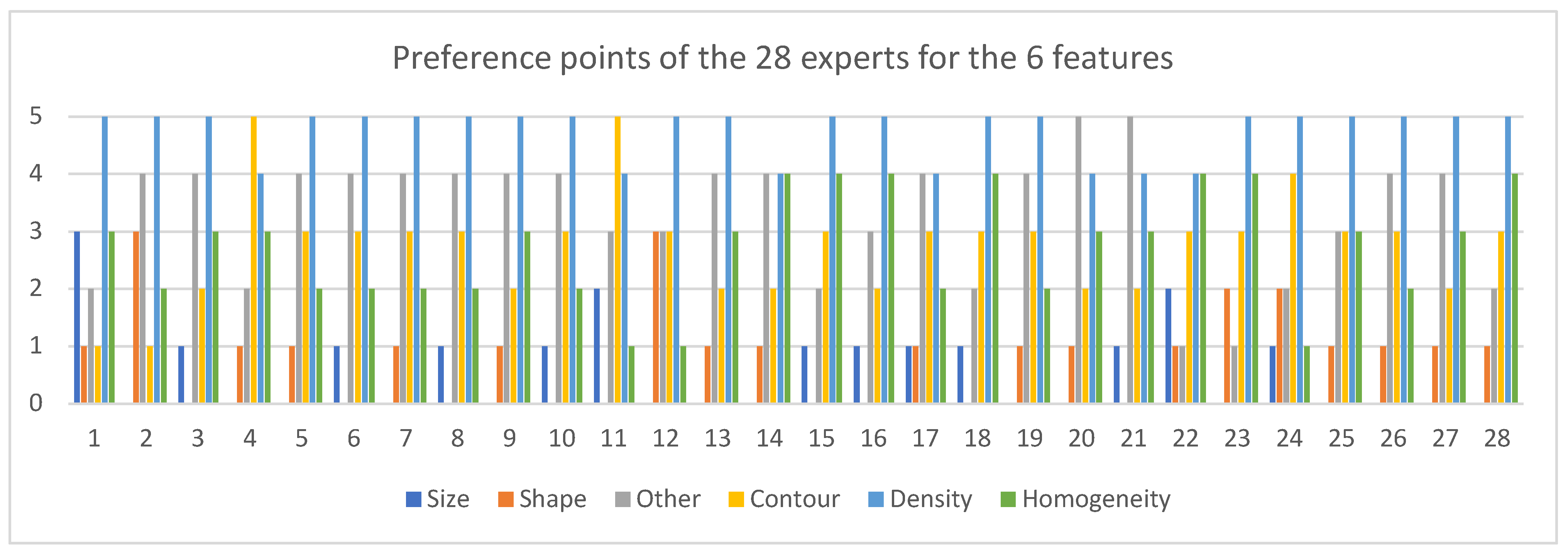
The sum of the preferred cases $a$ is shown in Figure 2 for all of the attributes, and all of the experts.

3.1.4. Sorting out the Inconsistent Experts, Based on Consistency Rate Calculation

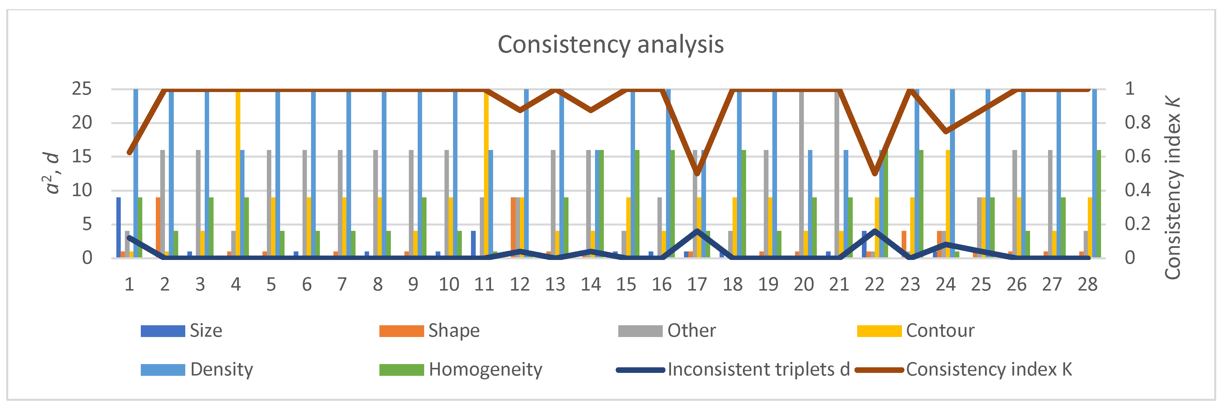
The number of inconsistent triplets $d$ and the consistency indices $K$, together with $a^2$ are shown in Figure 3. It is clearly visible that the consistency index of experts 1, 17, and 22 were below 75%, so in the final evaluation, the opinions of these experts were neglected.

3.1.5. Generating Preference Rates of Each Expert for Each Attribute

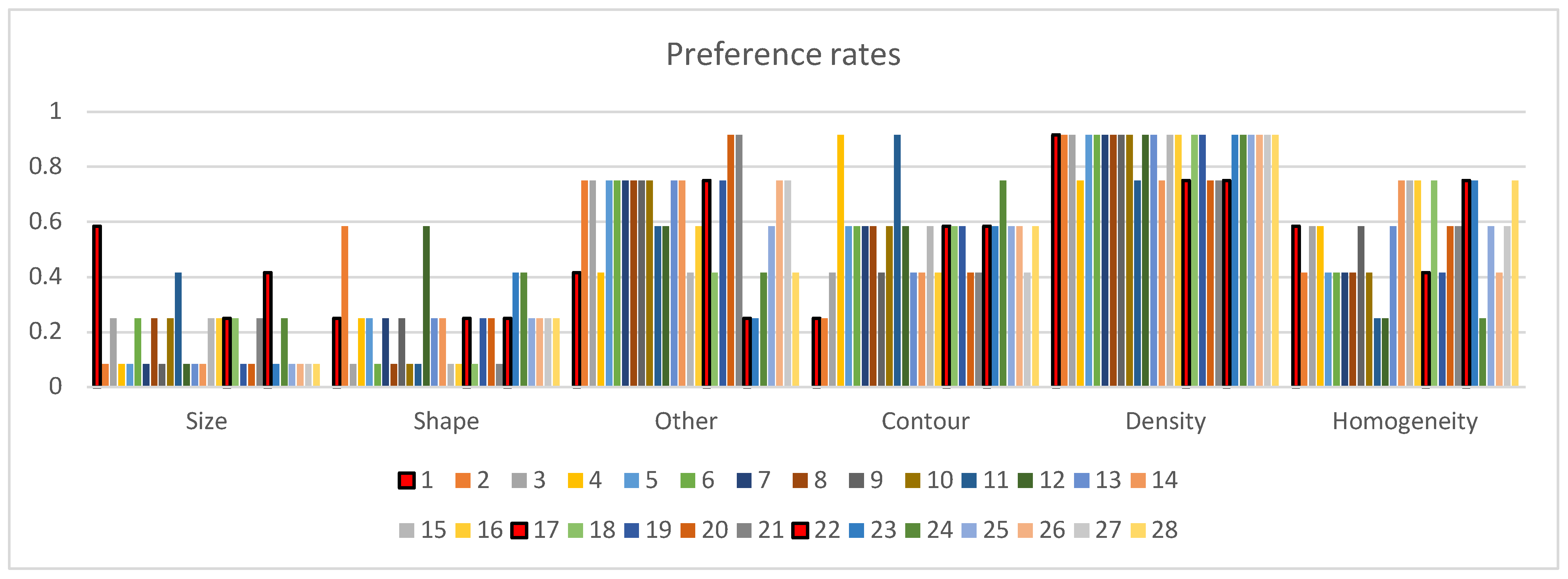
The preference rates $p$ of the experts were calculated according to Equation (3). Figure 4 contains the preference indices grouped according to the attributes (lower subplot), for better visibility.

3.1.6. Determining the Ranks of the Attributes in Decision Making

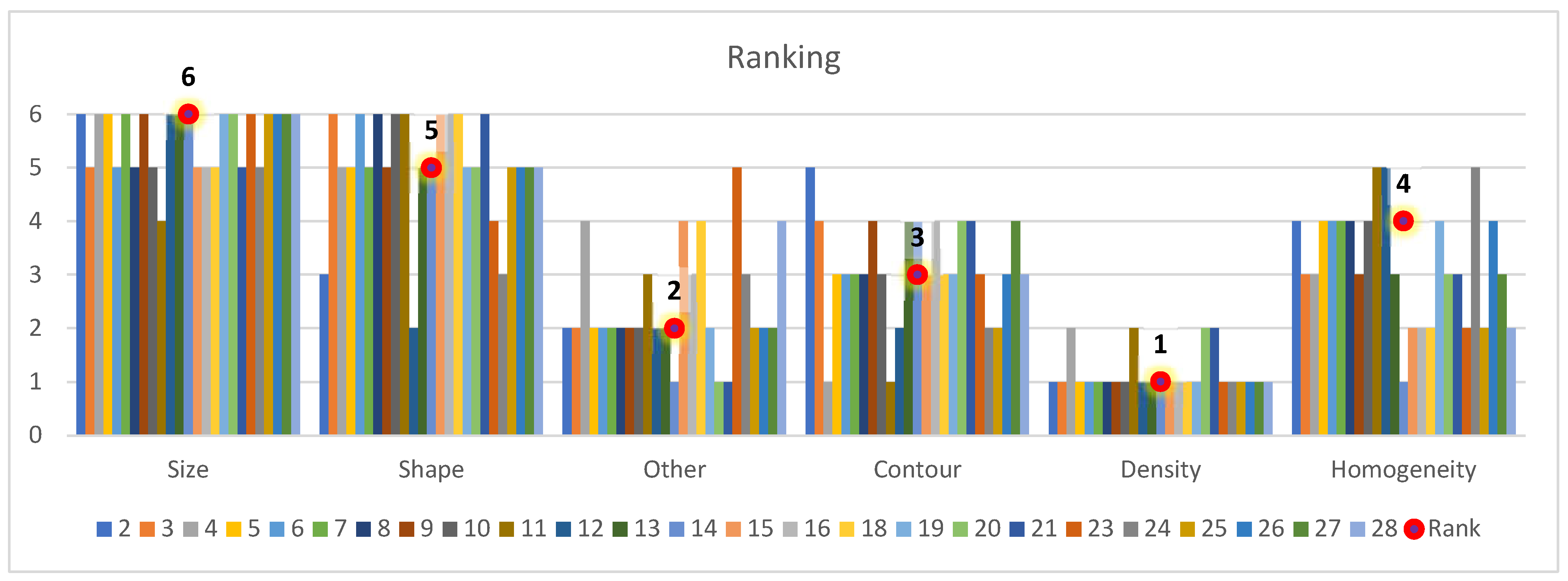
The preference rates were converted to rankings, according to Section 2.6.6. The rankings of the consistently answering experts are shown in Figure 5, together with the cumulative ranking of the attributes. The standard deviation of the rankings were ${\sigma }_{Size}=0.57$, ${\sigma }_{Shape}=1.04$, ${\sigma }_{Other}=1.02$, ${\sigma }_{Contour}=0.95$, ${\sigma }_{Density}=0.37$, and ${\sigma }_{Homogeneity}=1.07$. It can be seen that the ranking of density as the most important attribute has a very small deviation. In addition, the ranking of size as the least important attribute had a rather low standard deviation. The ranking of the other attributes was not that clear and sharp, they all had a standard deviation of about 1.

3.1.7. Calculating the Kendall Agreement Index

The Kendall agreement index [44] according to Equation (4) is $W=0.612$.

3.1.8. Building the Aggregated Preference Table

The final, aggregated preference table without the inconsistent experts is given in

Table 3. Aggregated preference table. The number of attributes is $n=6$, the number of consistent experts is $m=25$. The layout is similar to Table 1. Column $a$ is the total number of cases when the given attribute is preferred (this is shown in the later figures). Value $P$ is the aggregated preference rate (7), $u$ is the corresponding standard normal distribution value, and $Z$ is the weight in %, according to (8).

	Size	Shape	Other	Contour	Density	Homogeneity	$\mathit{a}$	$\mathit{P}$	$\mathit{u}$	$\mathit{Z}$
Size		10	0	0	0	1	11	0.16	−0.99	0
Shape	15		4	1	0	3	23	0.24	−0.71	12.9
Other	25	23		16	3	18	85	0.65	0.39	63.6
Contour	25	23	9		2	11	70	0.55	0.13	51.6
Density	25	24	23	23		25	120	0.83	1.18	100
Homogeneity	24	22	7	14	0		67	0.53	0.08	49.3
Sum	114	92	39	37	5	58

.

3.2. On Quantifying the Attributes

Of the attributes of size, density, shape regularity, contour sharpness, homogeneity, and other features, the first two can be easily calculated if the contour of the lesion is given.

3.2.1. Size

In medical practice, size is usually an approximate value of the largest distance between two points of the contour, it can be approximated by the larger size $D_L$ of the rectangular bounding box around the lesion. It might be also useful to determine the smaller size $d_L$ of the bounding box of the lesion.

As this attribute has a fixed formula (largest size of the lesion), which is accepted by the medical community, there is no reason to compare manual data to the machine calculated ones.

3.2.2. Density

The density can be calculated either as the mean $M_{\rho }$ or the median ${\mu }_{\rho }$ of the density values corresponding to the voxels within the boundaries of the lesion. In practice the mean value $M_{\rho }$ is used; this is also a closed formula once the contour of the lesion is given, thus there is also no need to compare the machine calculated values with the manually determined ones; the DICOM readers calculate the mean density of the selected area, and the radiologist experts use this value as the density.

3.2.3. Other Features

The attribute “other features” is only an umbrella expression for multiple attributes, it is not within the scope of this paper to go into further detail about this attribute.

The other three attributes “shape”, “contour”, and “homogeneity” are more complicated to quantify, they do not have a closed mathematical expression.

3.2.4. Contour

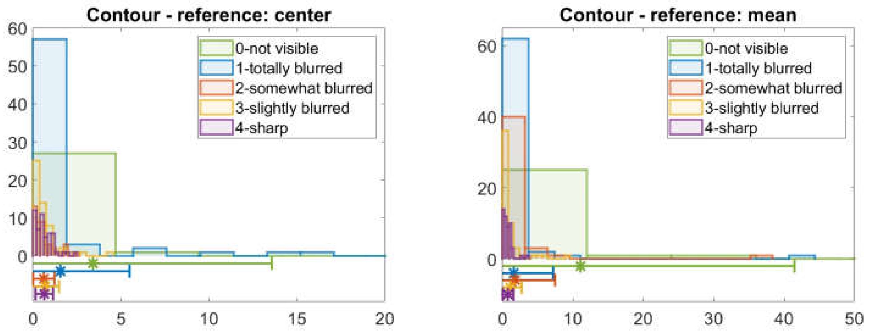
By contour sharpness, experts mean how close the average density of the lesion around its contour and the average density of the environment is to a step function, an ideally sharp edge would be the step function, and the flatter the transition the less sharp the contour. For this reason, we used the ratio of the average absolute density difference of voxels at about 10% of the smallest radius distance from the contour on both sides, and the density difference of healthy liver and the lesion, i.e.,

$$\mathrm{Contour}=\frac{\mathrm{Denstiy}\mathrm{difference}\mathrm{on}\mathrm{the}\mathrm{two}\mathrm{sides}\mathrm{of}\mathrm{the}\mathrm{contour}}{\mathrm{Density}\mathrm{difference}\mathrm{of}\mathrm{the}\mathrm{healthy}\mathrm{liver}\mathrm{and}\mathrm{the}\mathrm{lesion}}$$

(9)

Here, we used two types of lesion density as reference in the denominator, the average density of the lesion, and the average density of the lesion center within half of the radius. The first case will be referred to as the reference: mean, the second as the reference: center.

In addition, 245 pre-segmented images were manually evaluated and classified into five classes by a radiologist expert, with “4” being a sharp contrast and “1” barely visible contrast. If the lesion was not visible in the given phase, the category “0” was used. These classes are referred to as “experts’ classes”. For the same images, a numerical evaluation according to (6) was also performed for both references “center” and “mean”.

The histograms of all expert classes are given in Figure 6. Each expert class is denoted by different colors, hence the five histograms in the figure. If the suggested numerical value could represent the experts’ opinion, the histograms of these values should be significantly different for the five categories; moreover, they should have some kind of tendency similar to the expert categories 0 to 4 (or at least 1 to 4). To help to determine whether the suggested numerical values are able to represent the experts’ opinion, the mean values of each expert classes and their ±standard deviation environment are also shown in the figures below the histograms.

From the samples, it is not really possible to tell whether this seemingly plausible numerical representation could be used for the representation of the experts’ opinion. However, the first subplot of Figure 6 has a slightly better tendency in the center of the histograms, as well as their width, though their overlap is still too large. A study for determining the ideal distance from the contour should be carried out, to develop a better quantification of the attribute “contour”.

Figure 6. Histograms of the machine computed values meant to represent the attribute “contour” according to (6). The experts’ knowledge-based classification of the images has the five categories listed in the legend of the plot. Each expert category has one histogram. The bottom part of the image gives the mean value of the corresponding manual category with a marker * and the interval with length of the standard deviation left and right from the mean value is also indicated by the same color as the histogram. The distance of these intervals from the horizontal axis at 0 does not have any significance, it is only to make the intervals visible.

Figure 6. Histograms of the machine computed values meant to represent the attribute “contour” according to (6). The experts’ knowledge-based classification of the images has the five categories listed in the legend of the plot. Each expert category has one histogram. The bottom part of the image gives the mean value of the corresponding manual category with a marker * and the interval with length of the standard deviation left and right from the mean value is also indicated by the same color as the histogram. The distance of these intervals from the horizontal axis at 0 does not have any significance, it is only to make the intervals visible.

3.2.5. Shape

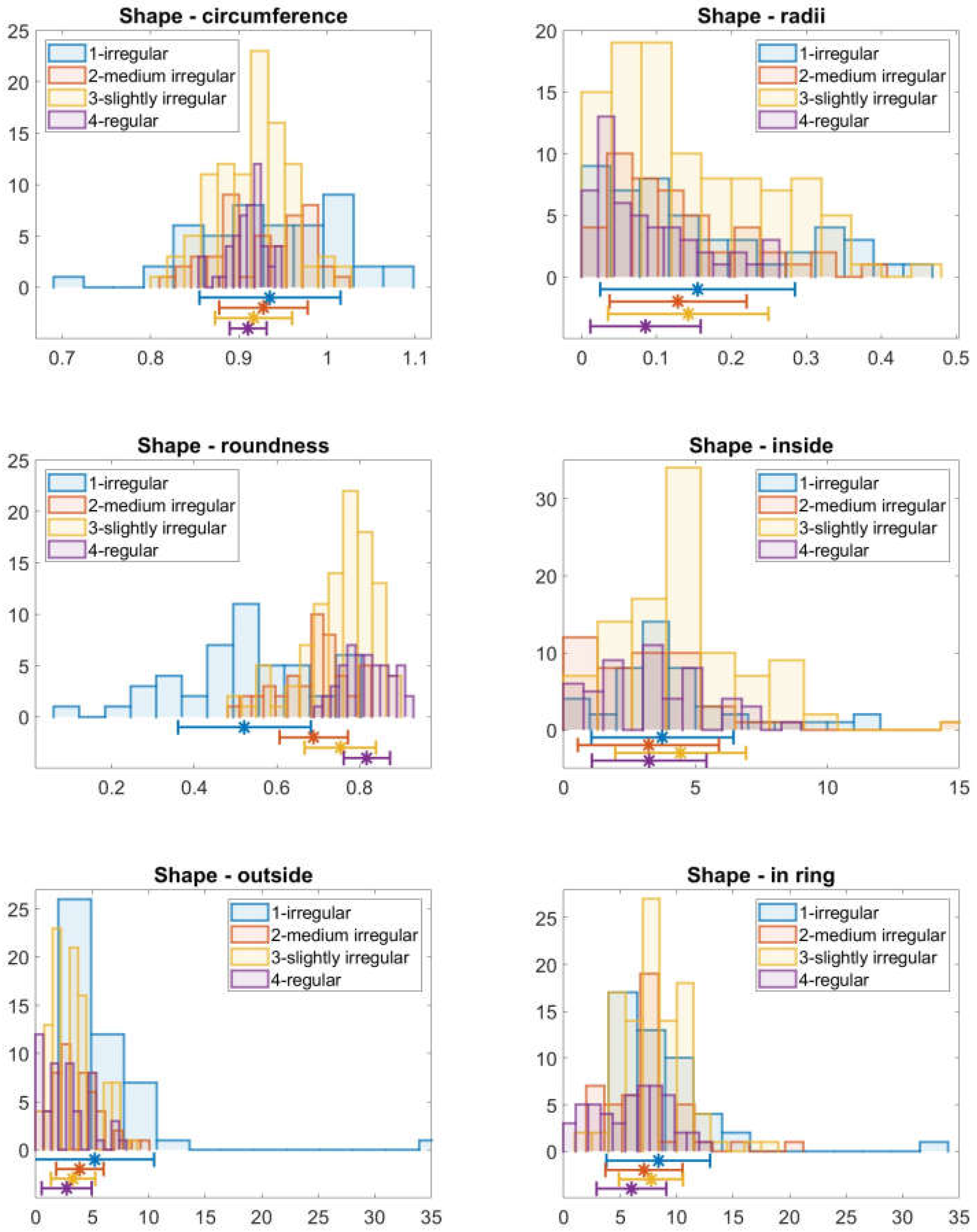
According to the experts, the shape of the lesion is considered regular (value “4”) if it is close to circular, and irregular “1” is a very much lobulated, elongated shape. The quantities considered for shape regularity are the following. As the most straightforward quantization of the shape, we calculated the ratio of the area and the circumference of the lesion and the difference of the larger and smaller size of the rectangular bounding box compared to the average radius

$${\mathrm{Shape}}_{\mathrm{circumference}}=\frac{\mathrm{Area}\mathrm{of}\mathrm{the}\mathrm{lesion}}{\mathrm{Circumference}\mathrm{of}\mathrm{the}\mathrm{lesion}},$$

(10)

$${\mathrm{Shape}}_{\mathrm{radii}}=\frac{\mathrm{Difference}\mathrm{of}\mathrm{the}x\mathrm{and}y\mathrm{dimensions}\mathrm{of}\mathrm{the}\mathrm{bounding}\mathrm{box}}{\mathrm{Diameter}\mathrm{of}\mathrm{the}\mathrm{lesion}},$$

(11)

The next quantity, which is used in mechanical engineering, is the roundness or circularity. It is the ratio between the largest deviation from the nominal circle of the object and the nominal radius,

$${\mathrm{Shape}}_{\mathrm{roundness}}=\frac{\mathrm{Maximum}\mathrm{absolute}\mathrm{deviation}\mathrm{from}\mathrm{the}\mathrm{nominal}\mathrm{circle}}{\mathrm{Radius}\mathrm{of}\mathrm{the}\mathrm{lesion}},$$

(12)

Moreover, for measuring lobularity and distinguishing between lobular and elliptical lesions, the number of times the contour leaves the 10% ring around the lesion’s nominal circle was calculated as well

$${\mathrm{Shape}}_{\mathrm{inside}}=\mathrm{Number}\mathrm{of}\mathrm{times}\mathrm{the}\mathrm{contour}\mathrm{leaves}\mathrm{the}10\%\mathrm{ring}\mathrm{towards}\mathrm{the}\mathrm{center},$$

$${\mathrm{Shape}}_{\mathrm{outside}}=\mathrm{Number}\mathrm{of}\mathrm{times}\mathrm{the}\mathrm{contour}\mathrm{leaves}\mathrm{the}10\%\mathrm{ring}\mathrm{outwards},$$

$$Shap{e}_{\mathrm{in}-\mathrm{ring}}=\mathrm{Number}\mathrm{of}\mathrm{times}\mathrm{the}\mathrm{contour}\mathrm{is}\mathrm{inside}\mathrm{the}10\%\mathrm{ring}.$$

Figure 7 shows the abovementioned three metrics and the number of times the contour is within the 5% ring around the nominal circle or leaves it toward the center or outside of the lesion.

The subplots are similar to those of Figure 6 in logic: each expert category has one histogram. The more distinguishable these categories are, the better the quantity represents the experts’ opinion. It can be seen that the mechanical engineering roundness gives a very good estimate of the expert opinion. The measures for representing the lobularity of the lesions, however, seem to be too strict, even the regular objects leave the environment of the nominal circle, so the proper limit to this environment, as well as the fitting of the nominal circle, needs to be studied further.

Figure 7. Expert opinion vs. computer calculated shape regularity values. The expert categories are represented by different colors, the machine calculated quantities are on the horizontal axis. The histograms of the machine calculated values corresponding to images from the four experts’ categories are plotted in the upper half of the images, while the mean value and standard deviation are denoted by a marker * and an interval around the mean value at the bottom of the plot, with the same color as the histogram.

Figure 7. Expert opinion vs. computer calculated shape regularity values. The expert categories are represented by different colors, the machine calculated quantities are on the horizontal axis. The histograms of the machine calculated values corresponding to images from the four experts’ categories are plotted in the upper half of the images, while the mean value and standard deviation are denoted by a marker * and an interval around the mean value at the bottom of the plot, with the same color as the histogram.

3.2.6. Homogeneity

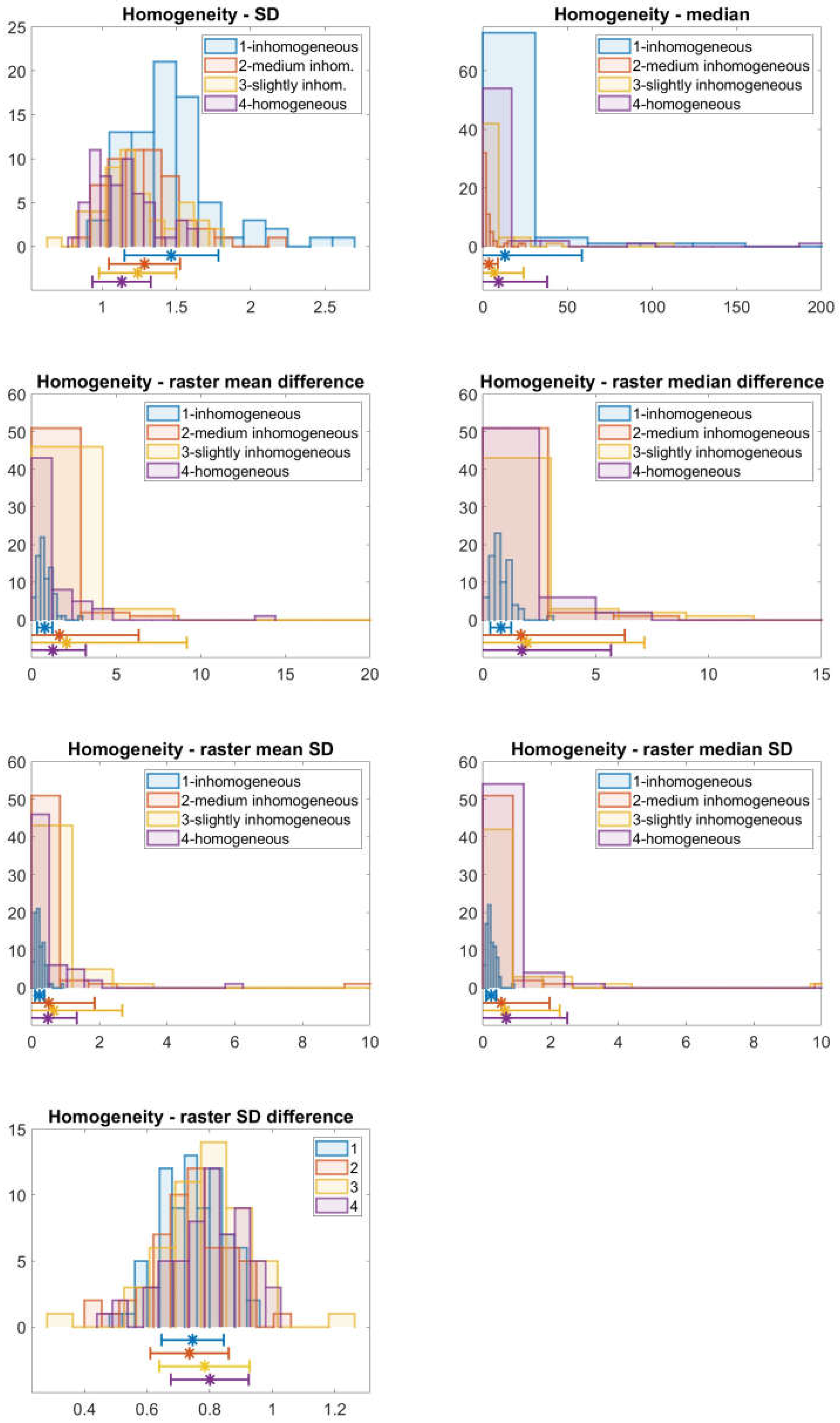
Based on discussions with the experts, the most complicated value is homogeneity. As even a healthy liver has a fine-grained inhomogeneity (which the medical experts consider as homogeneous), the classical homogeneity measures are not applicable. The radiologist experts understand the larger grained inhomogeneity or gradient within the lesion as inhomogeneity. Several quantities were measured: the mean, median, standard deviation, and the difference between the minimum and maximum density values of the healthy liver and the lesion, as well as the raster-averaged lesion (the raster-averaged lesion arose in the following way: the lesion’s bounding box was divided into 10 by 10 smaller rectangles (for smaller lesions, this number was smaller) and for those small rectangles, which contained part of the lesion, the statistical parameters, mean, median, and standard deviation were calculated). As we wanted to use easily computable and system independent quantities, the following experimental formulae were introduced to represent the experts’ classification.

$${\mathrm{Homogeneity}}_{\mathrm{SD}}=\frac{\mathrm{Standard}\mathrm{deviation}\mathrm{of}\mathrm{the}\mathrm{density}\mathrm{of}\mathrm{the}\mathrm{lesion}}{\mathrm{Standard}\mathrm{deviation}\mathrm{of}\mathrm{the}\mathrm{density}\mathrm{of}\mathrm{the}\mathrm{healthy}\mathrm{liver}},$$

(13)

$$\begin{array}{c}{\mathrm{Homogeneity}}_{\mathrm{median}}=\hfill \\ =\frac{\mathrm{Difference}\mathrm{between}\mathrm{the}\mathrm{mean}\mathrm{and}\mathrm{median}\mathrm{of}\mathrm{the}\mathrm{density}\mathrm{of}\mathrm{the}\mathrm{lesion}}{\mathrm{Difference}\mathrm{between}\mathrm{the}\mathrm{mean}\mathrm{and}\mathrm{median}\mathrm{of}\mathrm{the}\mathrm{density}\mathrm{of}\mathrm{the}\mathrm{healthy}\mathrm{liver}},\hfill \end{array}$$

(14)

$$\begin{array}{c}{\mathrm{Homogeneity}}_{\mathrm{raster}\mathrm{mean}\mathrm{diff}}=\hfill \\ =\frac{\mathrm{Difference}\mathrm{of}\mathrm{the}\mathrm{minimum}\mathrm{and}\mathrm{maximum}\mathrm{of}\mathrm{the}\mathrm{raster}\mathrm{mean}\mathrm{values}}{\mathrm{Mean}\mathrm{value}\mathrm{of}\mathrm{the}\mathrm{density}\mathrm{of}\mathrm{the}\mathrm{nodule}},\hfill \end{array}$$

(15)

$$\begin{array}{c}{\mathrm{Homogeneity}}_{\mathrm{raster}\mathrm{median}\mathrm{diff}}=\hfill \\ =\frac{\mathrm{Difference}\mathrm{of}\mathrm{the}\mathrm{minimum}\mathrm{and}\mathrm{maximum}\mathrm{of}\mathrm{the}\mathrm{raster}\mathrm{median}\mathrm{values}}{\mathrm{Median}\mathrm{value}\mathrm{of}\mathrm{the}\mathrm{density}\mathrm{of}\mathrm{the}\mathrm{nodule}},\hfill \end{array}$$

(16)

$${\mathrm{Homogeneity}}_{\mathrm{raster}\mathrm{mean}\mathrm{SD}}=\frac{\mathrm{Standard}\mathrm{deviation}\mathrm{of}\mathrm{the}\mathrm{raster}\mathrm{mean}\mathrm{values}}{\mathrm{Mean}\mathrm{value}\mathrm{of}\mathrm{the}\mathrm{density}\mathrm{of}\mathrm{the}\mathrm{nodule}},$$

(17)

$${\mathrm{Homogeneity}}_{\mathrm{raster}\mathrm{median}\mathrm{SD}}=\frac{\mathrm{Standard}\mathrm{deviation}\mathrm{of}\mathrm{the}\mathrm{raster}\mathrm{median}\mathrm{values}}{\mathrm{Median}\mathrm{value}\mathrm{of}\mathrm{the}\mathrm{density}\mathrm{of}\mathrm{the}\mathrm{nodule}},$$

(18)

$${\mathrm{Homogeneity}}_{\mathrm{raster}\mathrm{SD}\mathrm{diff}}=\frac{\mathrm{Median}\mathrm{of}\mathrm{the}\mathrm{standard}\mathrm{deviation}\mathrm{of}\mathrm{the}\mathrm{raster}\mathrm{mean}\mathrm{values}}{\mathrm{Standard}\mathrm{deviation}\mathrm{of}\mathrm{the}\mathrm{density}\mathrm{of}\mathrm{the}\mathrm{nodule}}.$$

(19)

According to Figure 8, however, the quantities combined from these parameters fail to characterize the homogeneity, so a deeper study dedicated to this question is required, though the standard deviation seems to be somewhat distinguishable for the four expert categories. It seems that the rastering, though it seems plausible, does not solve the problem of the distinguishing of the fine grained and coarse-grained homogeneity. Other methods, such as edge detection and edge counting might result in a better agreement with the experts’ opinion. During the discussions with the medical experts, however, a very interesting conclusion could be drawn. Even though they used the expression homogeneity and inhomogeneity, they meant different things by inhomogeneity. There are subcategories, such as spotted or puddle-like inhomogeneity, and ring-like inhomogeneity, and these categories have different roles in the diagnostic process, so these subcategories should also be represented for a more accurate decision support system.

4. Discussion

The consequent experts had a 0.612 Kendall inter-ranker reliability coefficient, which while being higher than 0.6, i.e., considered a good concordance, is still not very high. The reason for this could be the following:

According to our study, the experts use the density of the lesions as the most important attribute in the case of incidental findings of liver nodules in the abdominal CT examinations, and the size is the least important property. These quantities had a rather low variance (0.37 and 0.57) among the experts’ rankings, all the experts ranked the density as one of the first two places, and almost all the experts ranked the size as one of the last two places.

From Figure 5, as well as from their approximately 1 variance values, it can be also be seen that the other four attributes are ranked without a high concordance. This might be attributed to the fact that the borderline between the attributes contour, shape, homogeneity, and “other features” is different for each individual, even though the questionnaire gives a short description about the meaning of “other features”. More probably the ranking of the homogeneity, contour, shape, and other features depends on the actual case and the actual manifestation of the disease.

The attributes of density and shape are easy to quantify as soon as the lesion is marked in the CT images.

The other studied properties, namely the shape, contour, and homogeneity are not so clearly ordered; moreover, their quantification is also challenging. Several quantifying formulae were suggested and compared with the experts’ opinion regarding the regularity of the shape, the sharpness of the contour, and the homogeneity of the density distribution within the lesion. The shape can be quite well characterized by the roundness of the object. For the contour sharpness, the averaged density difference between the two sides of the borderline of the lesion versus the density difference of the lesion and the liver seems to be plausible, but the numerical results suggest this quantity is not good enough, and further study about this quantity is needed. Homogeneity is very hard to capture, not only because the CT images have a native, fine-grained inhomogeneity, but also because the experts understand different things under the same label “inhomogeneity”. Further research will be directed toward the more detailed quantization of the various meanings of inhomogeneity.

This implies that the attributes have two categories: a rather clear and easily represented class containing size and shape, and a class consisting of less clear and less easily interpreted expressions such as contour, shape, and homogeneity that cannot really be measured on a scale in one dimension.

5. Conclusions

Computer-aided diagnosis (CAD) is an ethically sensitive research area for multiple reasons. Due to the necessary protection of personal data, the number of samples is usually very limited. In addition, the question of accepting the results of a fully machine learning method as a reliable decision source, and the legal responsibility of such decisions are still a very much a debated area. This is the reason we suggest expert-based decision support methods as a valid alternative to the deep learning methods in CAD.

For building a proper CAD system that can be accepted by clinicians, it is really important to model the thinking of a human expert. This paper presents the primary step of the construction of an expert knowledge-based decision support method for multiple phases of liver CT analysis. This step determines which visible parameters of a CT image must be taken into consideration and, especially, their order of importance. This latter issue has been dealt with very little in the literature.

As a first step, the lesions and their manifestations throughout the CT phases were summarized.

Next, using pairwise comparison, the ranking of the previously selected radiology textbook attributes “size”, “shape”, “density”, “homogeneity”, “contour”, and “other features” was performed. According to the results, the most important feature is the density, and the least important is the size, while for the rest of the attributes, the order is “other”, “contour”, “homogeneity”, and “shape”; though here the variance of the ranking became larger than 1 based on the opinion of 25 consequent experts.

We proposed a weighting of features based on expert opinions that can be used in CAD systems. The weights were calculated using Guildford’s method. These weights are important for improving the accuracy of non-deep learning, conventional decision support systems.

As a last step, numerical quantities were suggested for the attributes “shape”, “contour”, and “homogeneity” on presegmented images. We showed that the quantification of these properties made by experts and by the machine, based on the lesion features, correlated for one of the suggested expressions for “shape”. However, for the other two features, “homogeneity” and “contour”, no numerical value could be attributed, as these expressions cover multiple phenomena. The quantifying of these features together with a more detailed study of the other attributes will be subject of further research.

References

- Miah, B.A.; Mohammad, A.Y. Detection of lung cancer from CT image using image processing and neural network. In Proceedings of the International Conference on Electrical Engineering and Information Communication Technology (ICEEICT), Savar, Bangladesh, 21–23 May 2015. [Google Scholar] [CrossRef]
- Skourt, B.A.; El Hassani, A.; Majda, A. Lung CT image segmentation using deep neural networks. Procedia Comput. Sci. 2018, 127, 109–113. [Google Scholar] [CrossRef]
- Aghamohammadi, A.; Ranjbarzadeh, R.; Naiemi, F.; Mogharrebi, M.; Dorosti, S.; Bendechache, M. TPCNN: Two-path convolutional neural network for tumor and liver segmentation in CT images using a novel encoding approach. Expert Syst. Appl. 2021, 183, 115406. [Google Scholar] [CrossRef]
- Hermann, Á.; Vámossy, Z. Image-based Lesion Classification using Deep Neural Networks. In Proceedings of the 2nd International Conference on Image Processing and Vision Engineering (IMPROVE 2022), Online, 22–24 April 2022; pp. 85–90. [Google Scholar] [CrossRef]
- Shu, X.; Yunyun, Y.; Boying, W. Adaptive segmentation model for liver CT images based on neural network and level set method. Neurocomputing 2021, 453, 438–452. [Google Scholar] [CrossRef]
- Lange, R.; Männer, R. Quantifying a critical training set size for generalization and overfitting using teacher neural networks. In Proceedings of the International Conference on Artificial Neural Networks (ICANN’94), Sorrento, Italy, 26–29 May 1994. [Google Scholar]
- Zadeh, L. Fuzzy sets. Inf. Control 1965, 8, 338–353. [Google Scholar] [CrossRef] [Green Version]
- Bektaş, N. Fuzzy Logic Based Rapid Visual Screening Methodology for Structural Damage State Determination of URM Buildings. In Proceedings of the 8th European Congress on Computational Methods in Applied Sciences and Engineering ECCOMAS Congress, Oslo, Norway, 5–9 June 2022. [Google Scholar] [CrossRef]
- Bukovics, Á.; Harmati, I.Á.; Kóczy, L.T. Fuzzy signature based methods for modelling the structural condition of residential buildings. In Soft Computing Applications for Group Decision-Making and Consensus Modeling; Collan, M., Kacprzyk, J., Eds.; Springer: Cham, Switzerland, 2018; pp. 237–273. [Google Scholar] [CrossRef]
- Lilik, F.; Nagy, S.; Kovács, M.; Szujó, S.K.; Kóczy, L.T. Interpolative decisions in the fuzzy signature based image classification for liver CT. In Proceedings of the 2021 IEEE International Conference on Fuzz Systems (FUZZ-IEEE), Luxembourg, Luxembourg, 11–14 July 2021. [Google Scholar] [CrossRef]
- Kovács, M.; Lilik, F.; Nagy, S.; Kóczy, L.T. On using fuzzy c-means clustering in the fuzzy signature concept classification of liver lesions. In Proceedings of the International Conference on Electrical, Computer, Communications and Mechatronics Engineering, Maldives, Maldives, 16–18 November 2022. [Google Scholar]
- Ji, H.; McTavish, J.D.; Mortele, K.J.; Wiesner, W.; Ros, P.R. Hepatic Imaging with Multidetector CT. RadioGraphics 2001, 21, S71–S80. [Google Scholar] [CrossRef] [PubMed]
- Chang, C.C.; Chen, H.-H.; Chang, Y.-C.; Yang, M.-Y.; Lo, C.-M.; Ko, W.-C.; Lee, Y.-F.; Liu, K.-L.; Chang, R.-F. Computer-aided diagnosis of liver tumors on computed tomography images. Comput. Methods Progr. Biomed. 2017, 145, 45–51. [Google Scholar] [CrossRef] [PubMed]
- Gunasundari, S.G.S.; Suganya Ananthi, M. Comparison and evaluation of methods for liver tumor classification from CT datasets. Int. J. Comput. Appl. 2012, 39, 46–51. [Google Scholar] [CrossRef]
- Huang, Y.L.; Chen, J.H.; Shen, W.C. Diagnosis of hepatic tumors with texture analysis in nonenhanced computed tomography images. Acad. Radiol. 2006, 13, 713–720. [Google Scholar] [CrossRef] [PubMed]
- Sayed, G.I.; Hassanien, A.E.; Schaefer, G. An automated computer-aided diagnosis system for abdominal CT liver images. Procedia Comput. Sci. 2016, 90, 68–73. [Google Scholar] [CrossRef] [Green Version]
- Kumar, S.S.; Moni, R.S.; Rajeesh, J. An automatic computer-aided diagnosis system for liver tumours on computed tomography images. Comput. Electr. Eng. 2013, 39, 1516–1526. [Google Scholar] [CrossRef]
- Hameed, R.S.; Kumar, S.S. Assessment of neural network based classifiers to diagnose focal liver lesions using CT images. Procedia Eng. 2012, 38, 4048–4056. [Google Scholar] [CrossRef] [Green Version]
- Chen, E.L.; Chung, P.C.; Chen, C.L.; Tsai, H.M.; Chang, C.I. An automatic diagnostic system for CT liver image classification. IEEE Trans. Biomed. Eng. 1998, 45, 783–794. [Google Scholar] [CrossRef] [PubMed] [Green Version]
- Balagourouchetty, L.; Pragatheeswaran, J.K.; Pottakkat, B.; Govindarajalou, R. Enhancement approach for liver lesion diagnosis using unenhanced CT images. IET Comput. Vis. 2018, 12, 1078–1087. [Google Scholar] [CrossRef]
- Huang, Y.; Chen, J.; Shen, W. Computer-aided diagnosis of liver tumors in non- enhanced CT images. J. Med. Phys. 2004, 9, 141–150. [Google Scholar]
- Mougiakakou, S.G.; Valavanis, I.K.; Nikita, A.; Nikita, K.S. Differential diagnosis of CT focal liver lesions using texture features, feature selection and ensemble driven classifiers. Artif. Intell. Med. 2007, 41, 25–37. [Google Scholar] [CrossRef] [PubMed]
- Gletsos, M.; Mougiakakou, S.G.; Matsopoulos, G.K.; Nikita, K.S.; Nikita, S.S.; Kelekis, D. A computer-aided diagnostic system to characterize CT focal liver lesions: Design and optimization of a neural network classifier. IEEE Trans. Inf. Technol. Biomed. 2003, 7, 153–162. [Google Scholar] [CrossRef]
- Frid-Adar, M.; Diamant, I.; Klang, E.; Amitai, M.; Goldberger, J.; Greenspan, H. GAN-based synthetic medical image augmentation for increased CNN performance in liver lesion classification. Neurocomputing 2018, 321, 321–331. [Google Scholar] [CrossRef] [Green Version]
- Bilello, M.; Gokturk, S.B.; Desser, T.; Napel, S.; Jeffrey, R.B.; Beaulieu, C.F. Automatic detection and classification of hypodense hepatic lesions on contrast- enhanced venous-phase CT. Med. Phys. 2004, 31, 2584–2593. [Google Scholar] [CrossRef] [PubMed]
- Diamant, I.; Hoogi, A.; Beaulieu, C.F.; Safdari, M.; Klang, E.; Amitai, M.; Greenspan, H.; Rubin, D.L. Improved patch-based automated liver lesion classification by separate analysis of the interior and boundary regions. IEEE J. Biomed. Health Inform. 2016, 20, 1585–1594. [Google Scholar] [CrossRef] [Green Version]
- Nayak, A.; Kayal, E.B.; Arya, M.; Culli, J.; Krishan, S.; Agarwal, S.; Mehndiratta, A. Computer-aided diagnosis of cirrhosis and hepatocellular carcinoma using multi-phase abdomen CT. Int. J. Comput. Assist. Radiol. Surg. 2019, 14, 1341–1352. [Google Scholar] [CrossRef]
- Sun, J.; Huang, L.; Shuai, H.; Huang, Y.; Lu, H.; Gao, F. Automatic computer-aided diagnosis of liver disease based on multi-cascade and multi-featured classifier. J. Med. Imaging Health Inform. 2015, 5, 322–325. [Google Scholar] [CrossRef]
- Lee, S.; Bae, J.S.; Kim, H.; Kim, J.H.; Yoon, S. Liver lesion detection from weakly-labeled multi-phase CT volumes with a grouped single shot multibox detector. In Medical Image Computing and Computer Assisted Intervention—MICCAI 2018; MICCAI 2018. Lecture Notes in Computer Science; Frangi, A., Schnabel, J., Davatzikos, C., Alberola-López, C., Fichtinger, G., Eds.; Springer: Cham, Switzerland, 2018; Volume 11071, pp. 693–701. [Google Scholar] [CrossRef] [Green Version]
- Seeram, E. Computed Tomography: Physical Principles, Clinical Applications, and Quality Control, 4th ed.; Elsevier: St. Louis, MO, USA, 2016; pp. 3–23. ISBN 9780323312882. [Google Scholar]
- Prokop, M. Principles of CT, Spiral CT and Multislice CT. In Spiral and Multislice Computed Tomography of the Body; Prokop, M., Galanski, M., Eds.; Thieme Verlag: Stuttgart, Germany, 2003; Charpter 1; pp. 6–7. [Google Scholar]
- Haaga, J.R.; Boll, D.T. CT and MRI of the Whole Body, 6th ed.; Elsevier Inc.: Philadelphia, PA, USA, 2017; pp. 4–13. ISBN 978-0-323-11328-1. [Google Scholar]
- DICOM Standard, Current Edition. Available online: https://www.dicomstandard.org/current, (accessed on 9 January 2023).
- General Data Protection Regulation. Available online: https://gdpr-info.eu/ (accessed on 6 February 2023).
- The HIPAA Privacy Rule. Available online: https://www.hhs.gov/hipaa/for-professionals/privacy/index.html (accessed on 6 February 2023).
- Bae, K.T. Intravenous Contrast Medium Administration and Scan Timing at CT: Considerations and Approaches. Radiology 2010, 256, 32–61. [Google Scholar] [CrossRef]
- Smithuis, R. CT Contrast Injection and Protocols, from Smithuis, R., & Van Delden, O. The Radiology Assistant. Available online: https://radiologyassistant.nl/more/ct-protocols/ct-contrast-injection-and-protocols (accessed on 19 December 2022).
- Schima, W.; Koh, D.M.; Baron, R. Focal Liver Lesions. In Diseases of the Abdomen and Pelvis 2018–2021; Hodler, J., Kubik-Huch, R., von Schulthess, G., Eds.; IDKD Springer Series; Springer: Cham, Switzerland, 2018; pp. 173–189. [Google Scholar] [CrossRef] [Green Version]
- Satoshi, K.; Osamu, M. Focal Hepatic Mass Lesions. In CT and MRI Imaging of the Body, 6th ed.; Haaga, J.R., Boll, D., Eds.; Elsevier: Philadelphia, PA, USA, 2017; Volume 2, pp. 1312–1375. [Google Scholar]
- Prokop, M.; van der Molen, A.J. Liver. In Spiral and Multislice Computed Tomography of the Body; Prokop, M., Galanski, M., Eds.; Thieme Verlag: Stuttgart, Germany, 2003; pp. 425–444. [Google Scholar]
- Nayantara, P.V.; Kamath, S.; Manjunath, K.N.; Rajagopal, K.V. Computer-aided diagnosis of liver lesions using CT images: A systematic review. Comput. Biol. Med. 2020, 127, 104035. [Google Scholar] [CrossRef] [PubMed]
- Ross, R.T. Optimum orders for the presentation of pairs in the method of paired comparisons. J. Educ. Psychol. 1934, 25, 375–382. [Google Scholar] [CrossRef]
- Spencer, J. Maximal Consistent Families of Triples. J. Comb. Theory 1968, 5, 1–8. [Google Scholar] [CrossRef] [Green Version]
- Kendall, M.G.; Babington Smith, B. The Problem of m Rankings. Ann Math Stat. 1939, 10, 275–287. [Google Scholar] [CrossRef]
- Dingman, H.F.; Guilford, J.P. A new method for obtaining weighted composites of ratings. J. Appl. Psychol. 1954, 38, 305–307. [Google Scholar] [CrossRef]
- Gray, H.; Lewis, W.H. Gray’s Anatomy of the Human Body, 20th ed.; Bartleby: New York, NY, USA, 2000. [Google Scholar]
- Hepatic Hemangiomas. Medscape. Available online: https://emedicine.medscape.com/article/177106-overview#a6 (accessed on 9 January 2023).
- World Cancer Research Fund International. Liver Cancer Statistics. Available online: https://www.wcrf.org/cancer-trends/liver-cancer-statistics (accessed on 9 January 2023).
Figure 1.
Flowchart of building our fuzzy signature-based decision support method. The green arrows indicate the target area of the present work.
Figure 2.
The results of the questionnaire for the 28 experts and 6 attributes. The different experts are denoted by the numbers 1 to 28 on the horizontal axis and the attributes by the colors of the columns, according to the legend at the bottom of the plot.
Figure 3.
The results, the number of inconsistent triples, as well as the consistency index derived from the questionnaire for the 28 experts and 6 attributes. The different experts are denoted by numbers 1 to 28 on the horizontal axis, the attributes by the color of the columns, according to the legend at the bottom of the plot. The number of inconsistent triples is shown with a solid dark blue line and the consistency rate is given by a solid dark red line, but the scale corresponding to the consistency index is on the right hand side of the plot.
Figure 4.
The preference rates for the 28 experts and 6 attributes. In the upper subplot the different experts are denoted by numbers 1 to 28 on the horizontal axis, the attributes by the color of the columns according to the legend at the bottom of the plot. The lower subplot contains the same information, but sorted according to the attributes. The inconsistent experts 1, 17, and 22 are denoted by a red column with black borderlines, the others have different colors in the lower subplot.
Figure 5.
Ranking of the 6 attributes: size, shape, other features, contour, density, and homogeneity for the 25 consistently answering experts. The different attributes are denoted on the horizontal axis, the experts are shown by the color of the columns, according to the legend at the bottom of the plot. The aggregated rank is given by the red dots and the numbers above the attributes.
Figure 8.
Expert opinion vs. computer calculated homogeneity values (10) to (16). The expert categories are represented as different colors, according to the legend. The upper part of the images shows the histograms of the distribution of the machine calculated quantities for the different experts’ categories, the lower part of the images shows their mean value by a marker *, and their standard deviation as the interval around the mean value. The same color is used for the histograms, mean, and standard deviation (the distance of the intervals from the horizontal axis is only for distinguishing them, it has no meaning).