
TSDNet: A New Multiscale Texture Surface Defect Detection Model †
1
School of Information Engineering, Zhengzhou University, Zhengzhou 450001, China
2
Henan Institute of Advanced Technology, Zhengzhou University, Zhengzhou 450003, China
3
School of Information and Communication Engineering, Beijing University of Posts and Telecommunications, Beijing 100876, China
4
School of Computer and Artificial Intelligence, Zhengzhou University, Zhengzhou 450001, China
*
Author to whom correspondence should be addressed.
†
This paper is an extended version of our paper published in ICTAI2022.
Appl. Sci. 2023, 13(5), 3289; https://doi.org/10.3390/app13053289
Submission received: 21 January 2023
/
Revised: 17 February 2023
/
Accepted: 1 March 2023
/
Published: 4 March 2023
(This article belongs to the Special Issue Application of Machine Vision and Deep Learning Technology)
Abstract
:Industrial defect detection methods based on deep learning can reduce the cost of traditional manual quality inspection, improve the accuracy and efficiency of detection, and are widely used in industrial fields. Traditional computer defect detection methods focus on manual features and require a large amount of defect data, which has some limitations. This paper proposes a texture surface defect detection method based on convolutional neural network and wavelet analysis: TSDNet. The approach combines wavelet analysis with patch extraction, which can detect and locate many defects in a complex texture background; a patch extraction method based on random windows is proposed, which can quickly and effectively extract defective patches; and a judgment strategy based on a sliding window is proposed to improve the robustness of CNN. Our method can achieve excellent detection accuracy on DAGM 2007, a micro-surface defect database and KolektorSDD dataset, and can find the defect location accurately. The results show that in the complex texture background, the method can obtain high defect detection accuracy with only a small amount of training data and can accurately locate the defect position.
1. Introduction
In the 1860s, human society began transforming from agricultural to industrial civilization. Machine production was gradually replacing manual labor. The development of the industry significantly promoted the progress of society. Since the 1950s, computer technology has made great progress and therefore was gradually combined with many other fields. In industrial manufacturing, surface defects are inevitable in the production process. There are many kinds of defects in the industry, such as scratches and cracks on steel surfaces, wear and stains on fabrics, scratches and impurities on glass products. The surface defects will not only affect the appearance and comfort of these products but also cause security incidents. At the same time, for factories, the low product quality will not only waste raw materials and increase production costs but also damage the reputation of the factory. Therefore, product quality control has always been the focus of attention. In the past, many factories used to use artificial methods to complete detection tasks, which are inefficient and unreliable. It will also bring greater human cost to the factories. With the development of computer technology, people focus on automatic detection technology and want to use the computer to complete the task of product quality control.
In recent years, with the integration and application of Informatization and industrialization, many links of industrial production have been replaced by computers. Computer vision technology has been successfully applied to the surface defect detection of industrial products.
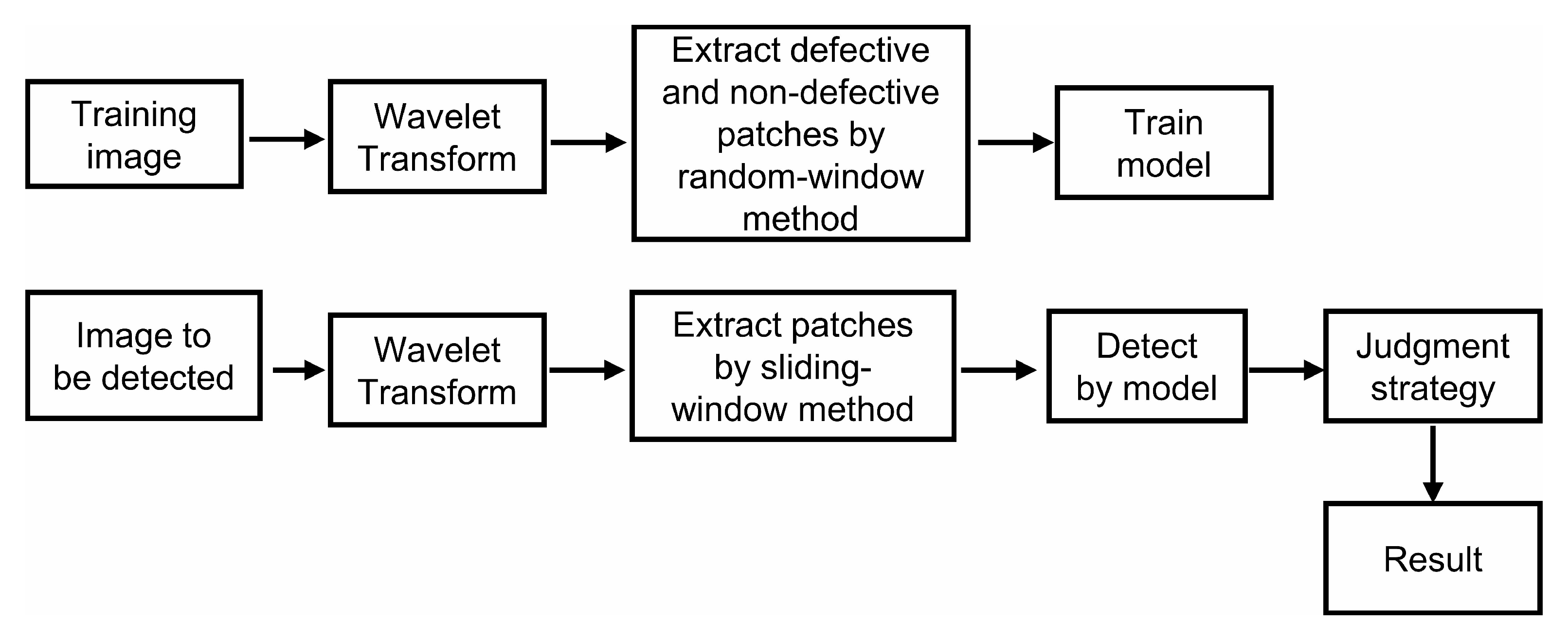
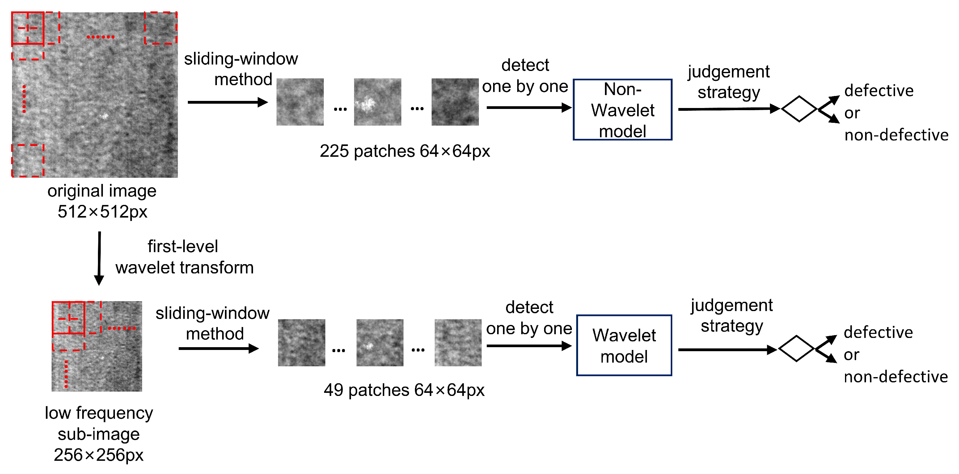
This paper proposes a texture surface defect detection approach based on CNN and wavelet transform, which can detect tiny defects in complex texture backgrounds. Compared with the existing approaches [1,2,3], this approach can achieve high detection accuracy with a small amount of training data. The general process of this approach is shown in Figure 1.
The main contributions of this paper are listed below:
- To solve the problem of tiny defect detection, a new method based on wavelet analysis and patch extraction is proposed, which can detect and locate many kinds of tiny defects in complex texture backgrounds with only a small amount of training data. Experimental results have verified its good performance.
- In the data preprocessing phase of our method, we propose a method which can automatically extract defective patches based on binary label images. Experiments show that this method can greatly reduce the workload of building a defective training dataset;
- A judgment strategy based on the sliding-window is proposed, which can improve the robustness of CNN networks. It can reduce the detection error probability in complex backgrounds.
The remainder of this paper is organized as follows. In Section 2, we firstly introduce the dataset and some theoretical background information, including the CNN network and theories of wavelet analysis. Then the procedures of our approach are introduced in detail, including the CNN network we used, the random-window method in the training phase, the sliding-window method, and judgment strategy in the defect detection phase. In Section 3, implementation details are illustrated. Experimental results are analyzed and compared with other well-known defect detection methods in Section 4. Finally, the conclusions are given in Section 5.
2. Related Work
2.1. Defect Detection
In traditional defect detection methods, people often design a specific algorithm for a type of defect to complete the defect detection task. For fabric defects detection, a detection method-based low-rank representation technique was proposed in the Ref. [4]. The technique can achieve good textile detection results without training data. Many researchers also use Gabor filters to detect fabric defects [5,6,7,8,9]. To detect jean fabric, the Ref. [5] proposed an improved algorithm based on the optimized Gabor filter. It selected the optimal filter from 24 Gabor filter banks by the one-dimensional image entropy algorithm and the two-dimensional image entropy algorithm. For wood defect detection, the work of [10] designed a novel method to detect and measure defects on the surface of trunks by using high-density 3D information. It used a segmentation algorithm to detect singularities on the trunk surface and a Random Forests machine learning algorithm to find the defect area. The results show that the method has high accuracy in defect detection and classification. For glass products, the Ref. [11] proposed a method to detect fibreglass components in the marine environment using terahertz waves. For steel products, a new Haar–Weibull variance model was proposed for steel surface defect detection in an unsupervised manner [12]. In the Ref. [13], the researchers proposed a robust sparse representation-based detection system to detect and classify hidden defects in radiographs of castings. In the Ref. [14], a multi-pair pixel consistency model was developed to represent the statistical relationship between each pair of pixels in a defect-free image. The algorithm developed based on this method can achieve a 100% defect detection rate.
The above studies used traditional defect detection methods, often designed for specific defects, and can obtain high accuracy. With the development of computing power and deep learning, current researchers prefer to use convolutional neural networks to detect defects automatically [15]. Convolutional neural networks have many advantages in the field of image processing [16], and gradually occupy the leading position in image classification [17].
In the Ref. [18], researchers used CNN to detect concrete cracks. The results show that the method performs well and can find concrete cracks in the actual situation. CNN is also used in the field of medical detection. In the Ref. [19], researchers trained an 18-layer CNN to detect glaucoma. In addition, there are also some people using CNN to detect fabric defects [20,21].
However, CNN also has some disadvantages, such as requiring a lot of training data and computing power. Furthermore, training a CNN using only original images may result in losing some indistinguishable features. In order to improve the performance of CNN networks, many researchers combine wavelet analysis with CNN and use the wavelet transform to analyze the multi-scale characteristics of data.
The Ref. [22] proposed a new method called MSCDAE, which uses only defect-free images for model training. The method utilizes CDAE to reconstruct image patches at different Gaussian pyramid levels and utilizes the reconstruction residuals of training patches to display detection results. The results show that the multimodal result fusion strategy can improve the defect detection performance. In the Ref. [23], the researchers used information in the wavelet domain as input to train a CNN model. Their method improves the learning ability, eliminates the overfitting phenomenon, and improves the efficiency of object detection. In the Ref. [24], Cui et al. fused multiple pyramid feature maps to enhance texture information in data preprocessing. These methods brought us some inspiration.
We have recently noticed some new defect detection methods, and they have achieved good performance. In the Ref. [25], a four-stage appearance defect detection model was proposed, which uses a simplified UNet model to segment candidate regions and builds a lightweight network based on candidate regions, achieving a fast inference speed. In the Ref. [26], a texture defect detection method based on principal component analysis and histogram-based outlier scoring was proposed, which requires only a small number of unlabelled samples and has low computational complexity. In the Ref. [27], Shen et al. developed a hybrid robust convolutional autoencoder to detect defection under noise. They designed a new FDD loss function to suppress the noises and constructed the PCDF module to enhance the robustness. In the Ref. [28], the researchers proposed a novel motor fault detection scheme based on one-class tensor hyperdisk. They used wavelet packet decomposition to extract feature tensors from motor novel multi-source signals for OCTHD training and used the decision function obtained from OCTHD training for detection.
2.2. Convolutional Neural Network
The convolutional neural network (CNN) is one of the representative algorithms of deep learning, which is already widely used in natural language processing [29,30], image recognition [31,32,33,34], image segmentation [35,36,37], and so on. CNN can automatically extract features from huge amounts of data and generalize the results to the same type of unknown data. In digital image processing, CNN can effectively extract features from the image, reduce the computation and improve the model’s efficiency.
2.3. Wavelet Analysis
Wavelet analysis is the most powerful tool in the field of signal and information processing, which is widely used in signal filtering, image denoising, image fusion, image edge detection and so on [38]. In image processing, wavelet transform is usually used to divide the image into different frequency bands. The image to be analyzed can be observed from multiple scales. In large-scale space, only the general appearance of the image can be observed; in small-scale space, we can observe the details of the image. The multi-scale observation method can extract some features that are not easily observed in a single scale.
A function is called a mother wavelet if it has finite energy and satisfy the condition given by Equation (1):
where is the Fourier transform of . Then we generate a wavelet-set from by dilating and translating Equation (2):
where is the dilating factor and is the translating factor. For the one-dimensional continuous function , its wavelet transform is as follows:
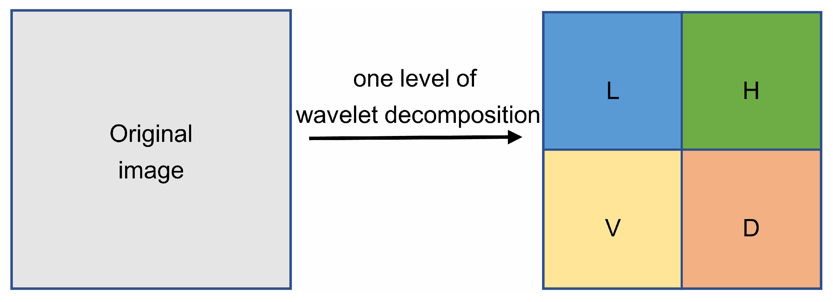
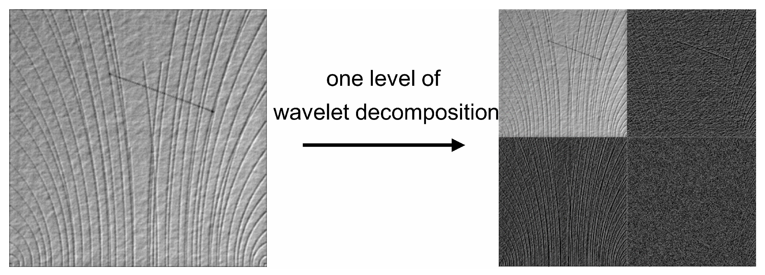
Image is a two-dimensional discrete signal. To transform it, we need to discretize the dilating factor and translating factor, and then extend the one-dimensional wavelet transform to two-dimensional. The multiresolution decomposition of an image is represented by a series of approximations and details in sub-images. Figure 2 illustrates the results of applying one level of wavelet decomposition, where L, H, V and D represent low-frequency coefficient, horizontal high-frequency coefficient, vertical high-frequency coefficient and diagonal high-frequency coefficient. The decomposition results of the real image are shown in Figure 3.
3. Method
3.1. System Overview
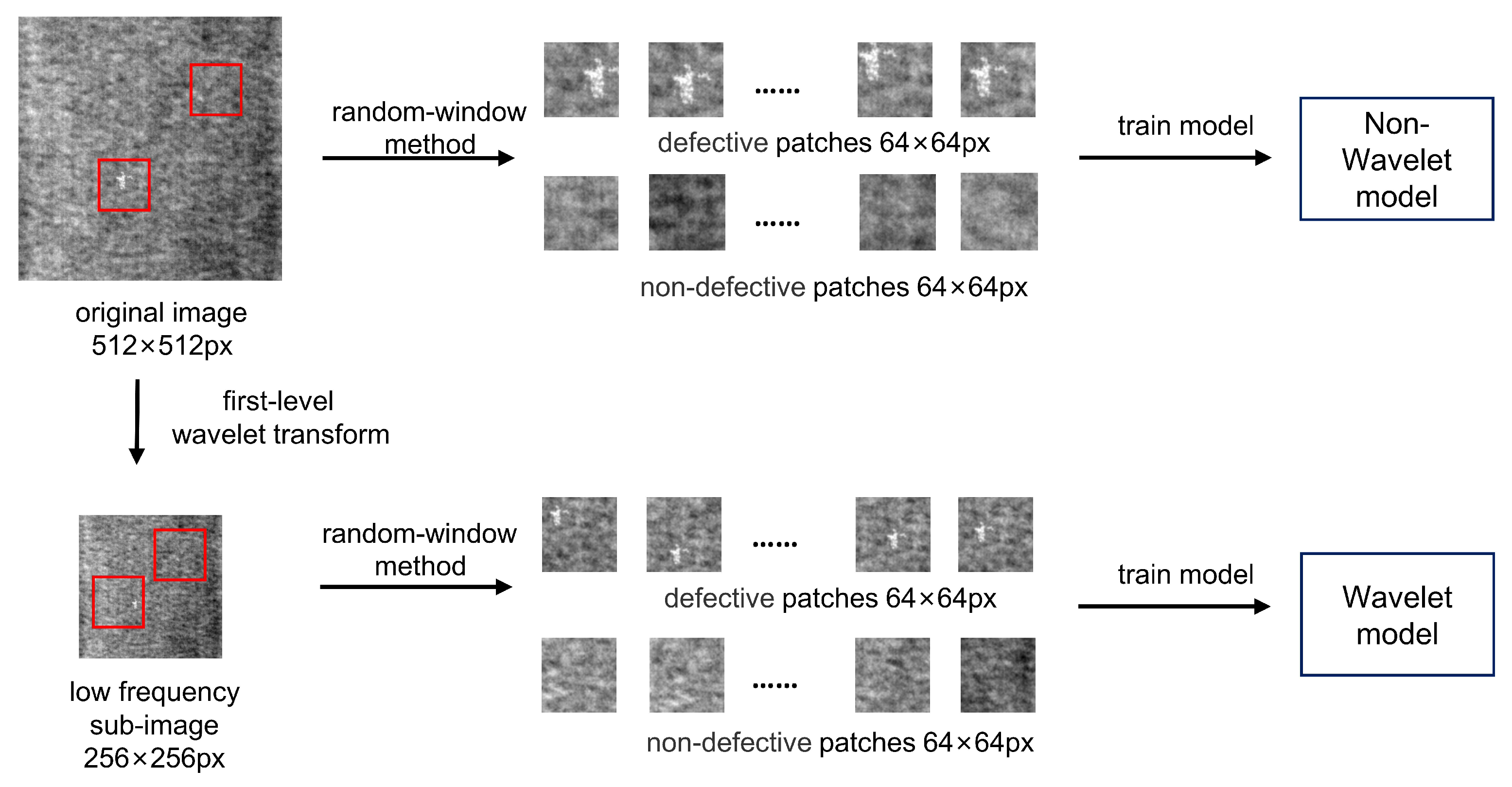
The dataset used in this approach is weakly labelled, and CNN can automatically extract and learn the features from the image, so the CNN network is applied in this work. In view of the previous work [1,2,3], because of the great differences between the background texture in the dataset, researchers have to use a lot of data to train the CNN network. However, In the field of deep learning, a large amount of training data is often difficult to get. Additionally, it will not only greatly increase the training time, but also the overall computation. To solve the above problems, this approach uses wavelet transform in the data preprocessing phase. The low-frequency part obtained after the image wavelet transform is the compression of the original image, which is only a quarter of the size of the original image, but the defects in the original image are still visible. Using small images can speed up model training and save resources. In order to speed up the training speed, reduce the training data and improve the detection accuracy, this approach uses the information in the wavelet domain as model input. In the model training phase, in order to overcome the challenge that the defect area is small, this paper proposes a random-window method to extract patches from the training images, and then uses the patches to train the CNN network. In the defect detection phase, this paper uses the sliding-window method and judgment strategy to solve the problem of background interference. First, we extract patches from the image to be detected using the sliding-window method. Then, all the patches are sent to the CNN network to judge whether there are defects. Finally, after considering the defect condition of the original image, the step of the sliding-window and other factors, we set a threshold. When the number of defective patches exceeds the threshold, the image is considered defective. By adjusting the threshold to find the best average accuracy, the best threshold is determined. Figure 4 and Figure 5 show the process of this approach in the model training phase and defect detection phase, respectively.
3.2. CNN for Defect Detection
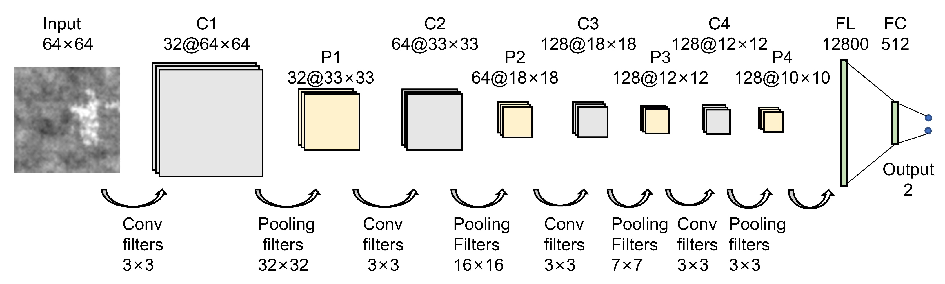
As shown in Figure 6, an 11-layer convolutional neural network is designed. The input of this network are patches, which come from the training image. The size of the patch is 64 × 64 pixels. The kernel size of each convolutional layer is always 3 × 3, and each convolutional layer is followed by a pooling layer. The size of the pooling filters decreases from 32 × 32 to 3 × 3, and the pooling strategy adopted in all the pooling layers is max-pooling, which can learn the edge and texture structure of the image. In addition, to keep the shape of the feature map, we apply the zero-padding strategy after each convolution. Finally, the dimension of the last fully connected layer is 2. The value of the output represents the probability of a defective image and a non-defective image, respectively.
3.3. Random-Window Method
In the model training phase, we need to extract defective and non-defective patches (64 × 64 pixels) from the training image, and then we use the patches to train the CNN networks. For the non-defective patches, they can be randomly extracted from the non-defective images. For the defective patches, they must be extracted near the defect area to ensure that the patches contain the defect area. There are 2100 defective images in the DAGM2007 dataset in total, and the defect area of some images is not obvious. Therefore, there will be a huge amount of work if the defective patches are extracted by humans. In addition, the process of extracting defect patches is actually a process of gathering defect parts, and the defected parts will occupy the main area of the patch. Training with these patches improves model recognition accuracy.
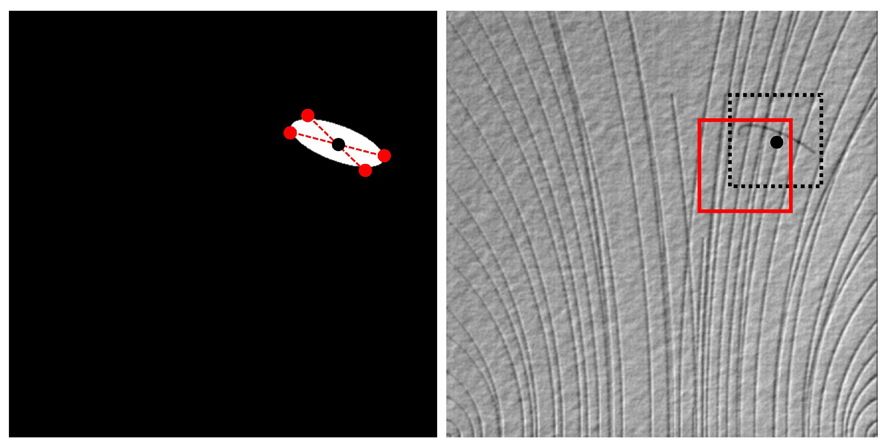
In Figure 7, it can notice that the label image in the DAGM2007 dataset is a binary image, the background is black, and the defect area is marked with a white ellipse. We can scan the label image along the x-axis and y-axis, respectively, and find four points which are tangent to the ellipse. According to this, we can find the center of the ellipse which is also the center of the random-window. Then we generate a series of random numbers as an offset of the random-window in the x-axis and y-axis directions, respectively. The value of the offset should match the defect area’s size and the random-window’s size to ensure that there are defect areas in the random-window. Results show that this random-window method is very effective under the appropriate offset and can automatically extract defective patches which are required in our approach.
3.4. Sliding-Window Method
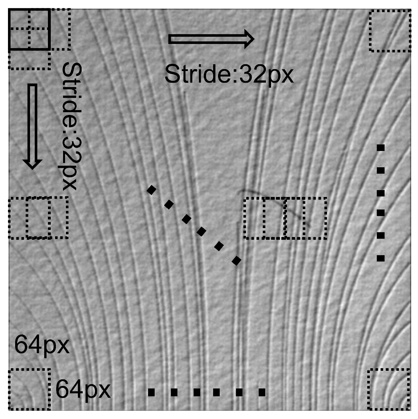
In the defect detection phase, each image to be detected needs to extract several patches (64 × 64 pixels) using the sliding-window method. Then the patches are detected one by one using the CNN networks. Using the sliding window can comprehensively extract image features, and combined with the proposed decision strategy it can effectively solve the problem of background interference. Figure 8 shows the segmentation method using the sliding-window. The size of the window is 64 × 64 pixels. In the DAGM2007 dataset, the window moves along the rows and columns over the image with a 32-pixel stride. In this way, 225 patches can be extracted from the original image (512 × 512 pixels), and 49 patches can be extracted from the low-frequency sub-image in the wavelet domain (256 × 256 pixels). In the micro-surface defect database, the stride is set to 16 pixels. Therefore the patch number of the low-frequency sub-image in the wavelet domain (240 × 320 pixels) is 204.
3.5. Judgment Strategy
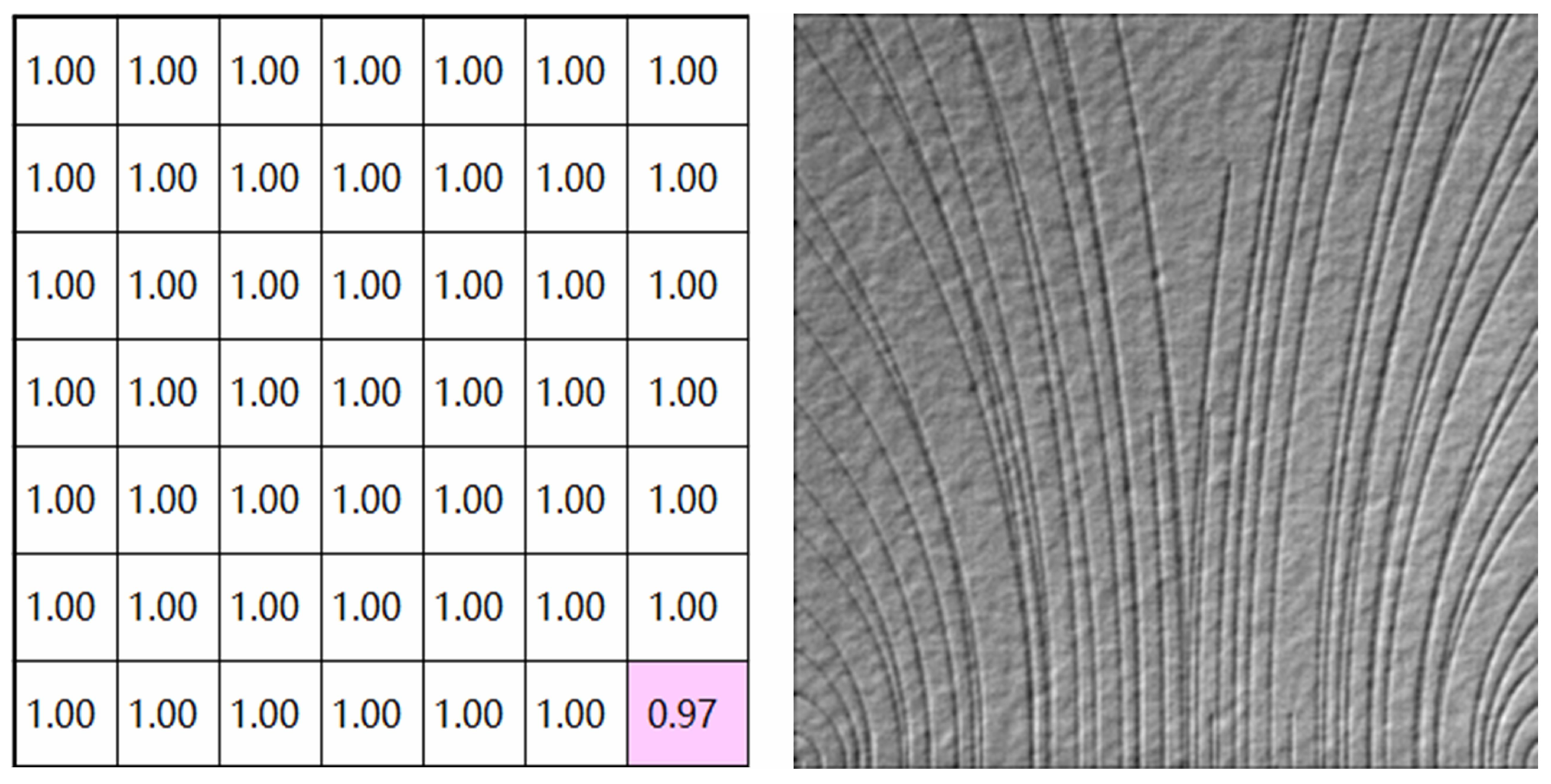
In the defect detection phase, the patches are detected one by one using the CNN networks. After that, each patch corresponds to an output, which also represents the defect probability of the patch. As shown in Figure 9, each element of the matrix represents the probability that there are no defects in the patch. On the right of Figure 9 is the low-frequency sub-image in the wavelet domain (256 × 256 pixels) to be detected. It can be seen that our method can not only judge whether there are defects in the image, but also roughly find the location of defects. It should be noted that the size of the sliding-window is 64 pixels, and the step is 32 pixels in DAGM, so there is partial overlap between patches. That means the element position in the probability matrix does not match the position of the patch in the image.
If the prediction probability of 0.5 is used as the threshold to distinguish defective images from non-defective images, it can be found that the element in the lower right corner of the probability matrix of Figure 9 is 0.23, which means the CNN model predicts the patch is defective. However, as you can see from the right image in Figure 9, the patch in the lower right corner is non-defective. In our judgment strategy, the prediction error of a few patches will not affect the final judgment. Because of the overlap in the process of extracting patches by the sliding-window method, at least four defective patches are extracted from each defect area in DAGM. In the judgment strategy of the defect detection stage, a threshold can be determined by comprehensively considering the size of the defect area, the accuracy of model, the step of the sliding-window and other factors. When the number of defective patches is greater than the threshold, it is considered that the image to be detected is defective. Under this strategy, the defect detection method is robust to background interference. Figure 10 shows a non-defective image and its probability matrix as a comparison.
4. Experiments
4.1. Dataset
4.1.1. DAGM2007
The German Association for Pattern Recognition (DAGM) and the German Chapter of the European Neural Network Society (GNNS) launched a competition for industrial defect detection. They provided a dataset called “Weakly Supervised Learning for Industrial Optical Inspection”, including 10 classes’ images. The first six classes of images are composed of 150 defective images and 1000 non-defective images, while the last four kinds of images are composed of 300 defective images and 2000 non-defective images. The image samples of 10 classes with size 512 × 512 pixel are shown in Figure 11, where each of them is generated by different texture models and defect models, and the defect areas have been circled with ellipse labels. At present, many algorithms have been tested on this dataset, but there is still room for improvement. The main reason is that: (1) The defect area is only weakly labelled by an ellipse, which means there are some non-defective images in the ellipse; (2) compared with the whole image, the defect area is very small, and most of them are not obvious; and (3) the background texture of some images varies a lot.
4.1.2. Micro-Surface Defect Database
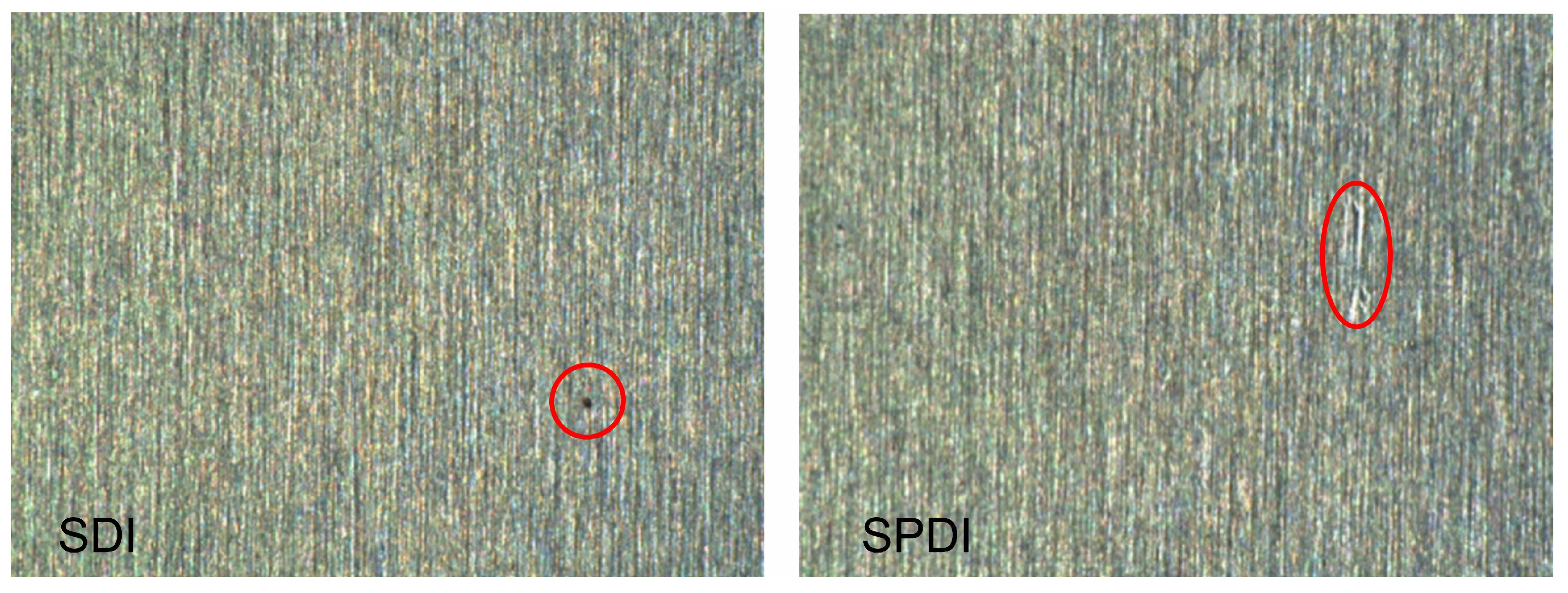
The micro-surface defect database was collected by Song et al. [39]. There are two classes of images in this dataset, where one is called the spot-defect image (SDI) and the other is called the steel-pit-defect image (SPDI). There are 20 images in the first class and 15 images in the second class, where some images may contain more than one defect. The image samples of this dataset with a size of 640 × 480 pixels are shown in Figure 12, where the defect area is marked with a red ellipse. In the silicon steel strip, the spot-defect is one of the most common defect types in the micro-surface defect, and the defect in SDI is only 6 × 6 pixels. As for SPDI, the defect is a strip-shaped hollow, and the defect area is relatively bright. It can be found that there are many strong interferences in the background of this kind of image.
4.1.3. KolektorSDD Dataset
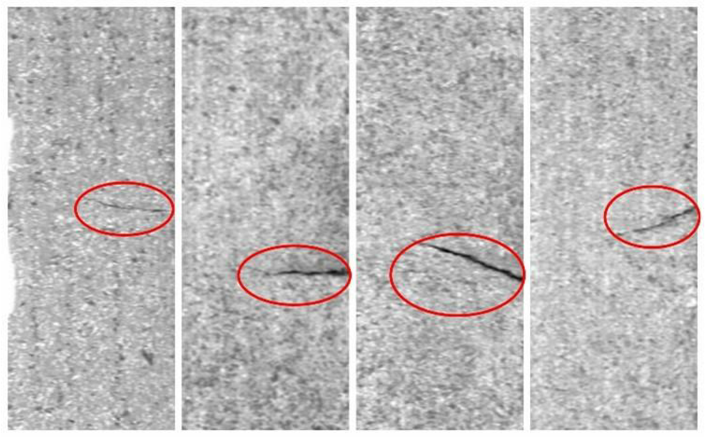
The KolektorSDD dataset [40] contains 50 folders, each containing about eight images of metal surfaces with their corresponding labels. The entire dataset has 399 images, of which 52 are defective and 347 are non-defective. The image’s width is 500 pixels, and the height varies from 1240 pixels to 1270 pixels. A partial image of the dataset is shown in Figure 13, where the defect area is marked with a red ellipse. Most of the defects in this dataset are obvious, but there are many fine-grained spots in the image, which are easy to interfere with defect detection. In addition, there are only 52 defective pictures, which is less than the non-defective data. Thus, the data enhancement is required.
4.2. Experiment Settings
Our model was trained on a Windows computer with NVIDIA GTX1660ti 6G GPU. The language utilized for the proposed method was Python 3.7. The CNN network was trained in the framework of Keras 2.0.6 and Tensorflow 1.3.0.
According to the work of He et al. [41], the Kaiming Initialization method is used in this model, which means the weight parameters are initialized from a Gaussian distribution with mean 0 and variance, and here N is the number of connections between two layers. As for the activation function, the ReLU function is used in each layer except the last layer. The last layer uses the Softmax function as the activation function.
As for the loss function, we chose the cross-entropy function to evaluate the difference between the predicted probability and the actual probability. In the gradient descent algorithm, the widely used Adam optimization algorithm was selected. The initial learning rate was set to 0.000001, and in order to reduce the training time of the model and prevent the oscillation of loss, the learning rate decay method was also applied.
This method was verified on the DAGM2007 dataset, the micro-surface defect database, and KolektorSDD dataset. We trained two CNN networks for each class of image with the same parameters, where one uses the original image, and the other uses the high-frequency sub-image after one-level wavelet decomposition of the original image.
4.2.1. DAGM2007
There are 150 defective and 1000 non-defective images in the first six classes of the DAGM2007 dataset. In the last four classes, the numbers are 300 and 2000, respectively. For the defective patches in the training set, first, we apply the random-window method to extract 6–10 defective patches with a size of 64 × 64 pixels from each defective image. Then the patches are increased by rotations and radial symmetry. For the non-defective patches, we extract patches from non-defective images randomly. Finally, the training set for our wavelet model has about 1800 defective patches and 3200 non-defective patches in the first six classes, and about 3400 defective patches and 7200 non-defective patches in the last four classes. The image and patch distribution of each class are shown in Table 1 and Table 2, respectively.
4.2.2. Micro-Surface Defect Database
In this dataset, we still use the random-window method to create defective patches and non-defective patches. In our wavelet model, we extracted 885 defective patches (64 × 64 pixels) and 1146 non-defective patches (64 × 64 pixels) from SDI. As for SPDI, the number is 703 and 873. In the defect detection phase, here we set the sliding-window step size to 16 pixels, so each defect area will be extracted by at least 9 patches. For the defect threshold in SDI, when the number of defective patches in an area was more than 3, we judged that there were defects. Because the defect in SDPI is bigger than the SDI, we set the defect threshold to 4 in the SDPI.
4.2.3. KolektorSDD Dataset
Since the heights of the images in the KolektorSDD dataset are inconsistent, we first scale the images to 1024 × 256 to ensure that the images and labels are scaled with the same regularity. The dataset is divided into a training set (containing 256 non-defective and 36 defective) and a test set (containing 91 non-defective and 16 defective). After that, a random window method is used to extract 64 × 64 patches from the defective and non-defective images. Since the defect-free data are relatively small, the data enhancement methods of up–down, left–right, and inversion are adopted. A total of 798 defect-free patches and 684 defect patches were extracted, and all patches were 64 × 64 pixels in size. In the defect detection stage, we set the sliding window step size to 32 pixels and the judgment threshold to 0. As long as there is a patch abnormality, it will be judged as defective.
4.3. Results and Discussion
4.3.1. DAGM2007
As for the evaluation criteria, we use the true positive rate (TPR), true negative rate (TNR) and average accuracy rate (AVEACC) as metrics. These metrics are defined as follows:
where TP and FN refer to the number of defective images detected as defective and non-defective, respectively. TN and FP refer to the number of non-defective images detected as non-defective and defective, respectively. AVEACC is the total number of correctly predicted images in all classes divided by the total number of images in all classes. TN refers to the number of non-defective images detected as non-defective in class i.
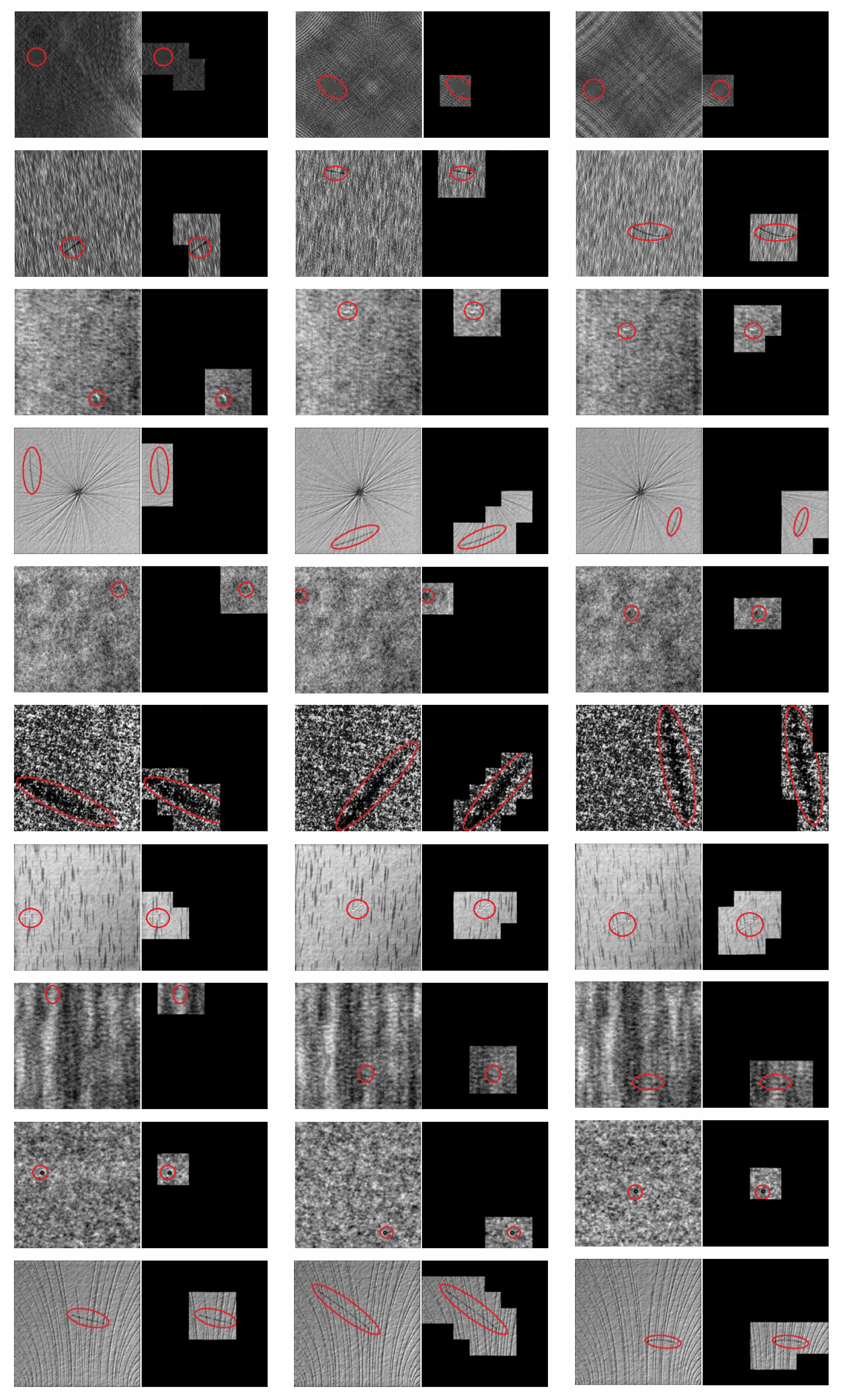
Figure 14 illustrates our detection results of this method. The non-defective areas are covered by the black image in the results. It should be noted that the step of the sliding-window method in the detection phase is 32 px, which is less than the size of patches 64 px, so some areas of the image to be detected may be judged as both defective and non-defective at the same time. The results shown in Figure 14 consider the above situation as defective. It can be found that this method can detect small defects in the image with large texture differences in the background, and also can roughly determine the location of the defects.
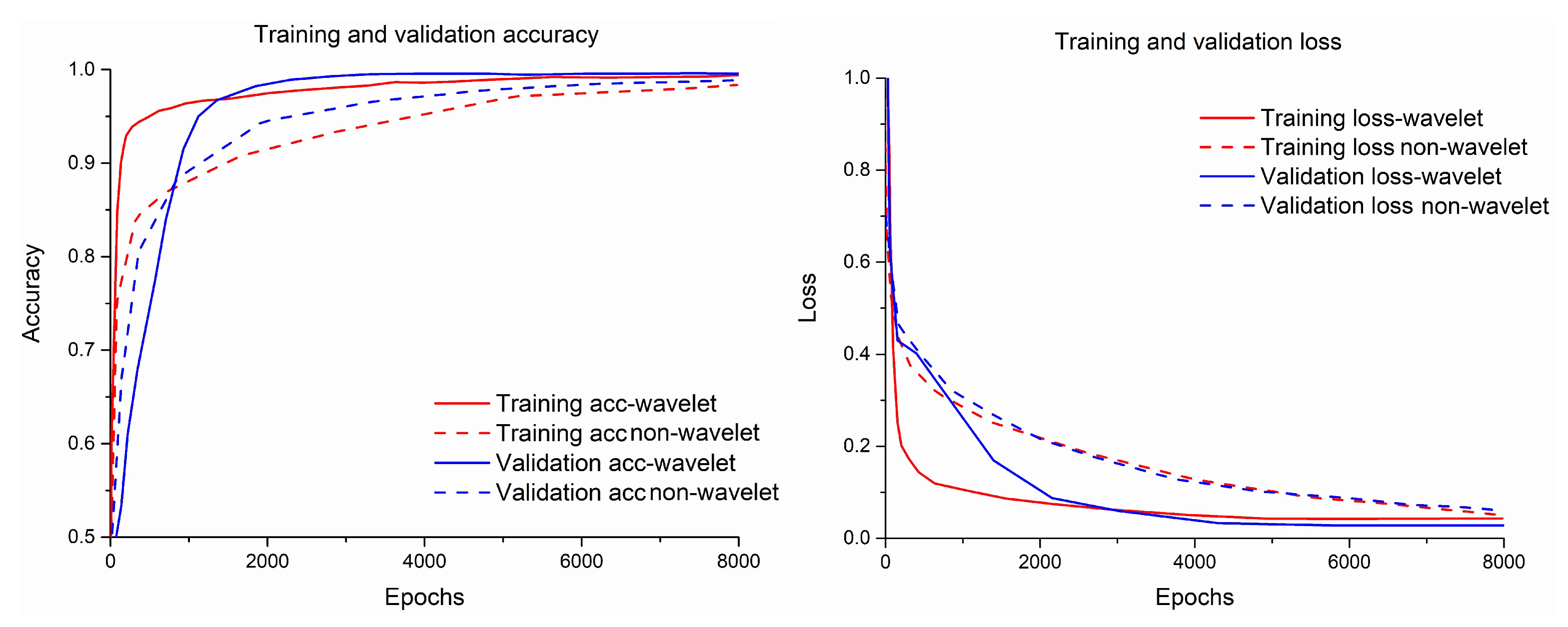
To show the high efficiency of this approach, we trained the wavelet and non-wavelet models for each class of the DAGM2007 dataset under the same parameters. Here we take the class 10 images as an example. Figure 15 shows the accuracy curve and loss curve of the wavelet model and non-wavelet model during the training process. It can be found that the wavelet model is better than the non-wavelet model in accuracy and learning speed.
As for the accuracy of detection, the results and comparisons are shown in Table 3. Table 3 shows the TPR and TNR of each class in the wavelet model and non-wavelet model. It can be seen from the comparison between the wavelet model and non-wavelet model that except Class 8, the performance of the wavelet model is better than the non-wavelet model in the same training environment. Compared with the work of other researchers, the average accuracy of our wavelet model is only slightly lower than the method In the Refs. [1,2,25]. In terms of TPR and TNR, the performance of this method is better than the traditional defect detection methods proposed in the Refs. [42,43,44] in most cases, similar to the CNN model proposed in the Ref. [3], slightly lower than the method proposed in the Refs. [1,2,25].
Table 4 shows the comparison between our method and others in accuracy and the amount of training data. Both the methods proposed in the Refs. [1,2,3] and our method use CNN to detect defection. Although the accuracy of our method is not much higher than the above three, the amount of training data in our method is far less than theirs. For the first six classes of images, our wavelet model has 5037 patches (64 × 64 pixels) on average for each class. The total training set had 20,631,552 pixels in each class. In the Refs. [1,2,3], the total training set had 209,190,912, 867,631,104 and 221,729,792 pixels in each class, respectively. As for the last four classes of images, the numbers of our model and that of the Ref. [1] were 40,710,144 and 419,430,400 pixels, respectively.
Through comparison, it can be found that although the average accuracy of the Ref. [1] is 0.4% higher than our method, the total training pixels In the Ref. [1] is 10 times bigger than ours. In the Ref. [2], the average accuracy is 0.5% higher than our method, but their total training pixels is 42 times bigger than ours. Compared with the Ref. [2], the average accuracy of our method is not only 0.1% higher than that of them, but the total pixels of our training set is also one-tenth of them. In the field of deep learning, models usually have better performance on the trained data. Therefore, the extensive use of data as training sets can help to improve the prediction accuracy of their model, but it will also increase the amount of calculation and the training time. The Ref. [25] proposed a four-stage appearance defect detection model which can achieve high detection accuracy. They used U-Net to segment those candidate defect regions the image and then make corrections and decisions, while ours only uses the basic convolutional neural network. In contrast, our focus is on data processing and judgment, and the complexity of the model is low.
4.3.2. Micro-Surface Defect Database
In this dataset, we use Recall and Precision as evaluation criteria. These metrics are defined as follows:
where TP and FN refer to the number of defective areas detected as defective and non-defective, respectively; and FP refers to the number of non-defective areas that are detected as defective. Table 5 illustrates the performance of our method in detecting micro-surface defect databases. Figure 16 illustrates the real detection results. As above, the area detected as non-defective is covered with a black image. It can be seen from the results that our method has good detection performance for tiny defects (6 × 6 pixel) in a complex background, and only a small amount of data is needed to meet the training requirements of the model.
4.3.3. KolektorSDD Dataset
In this dataset, we still use recall and precision to evaluate model performance, which are defined as Equations (7) and (8). Table 6 illustrates the performance of our method in detecting the KolektorSDD dataset.
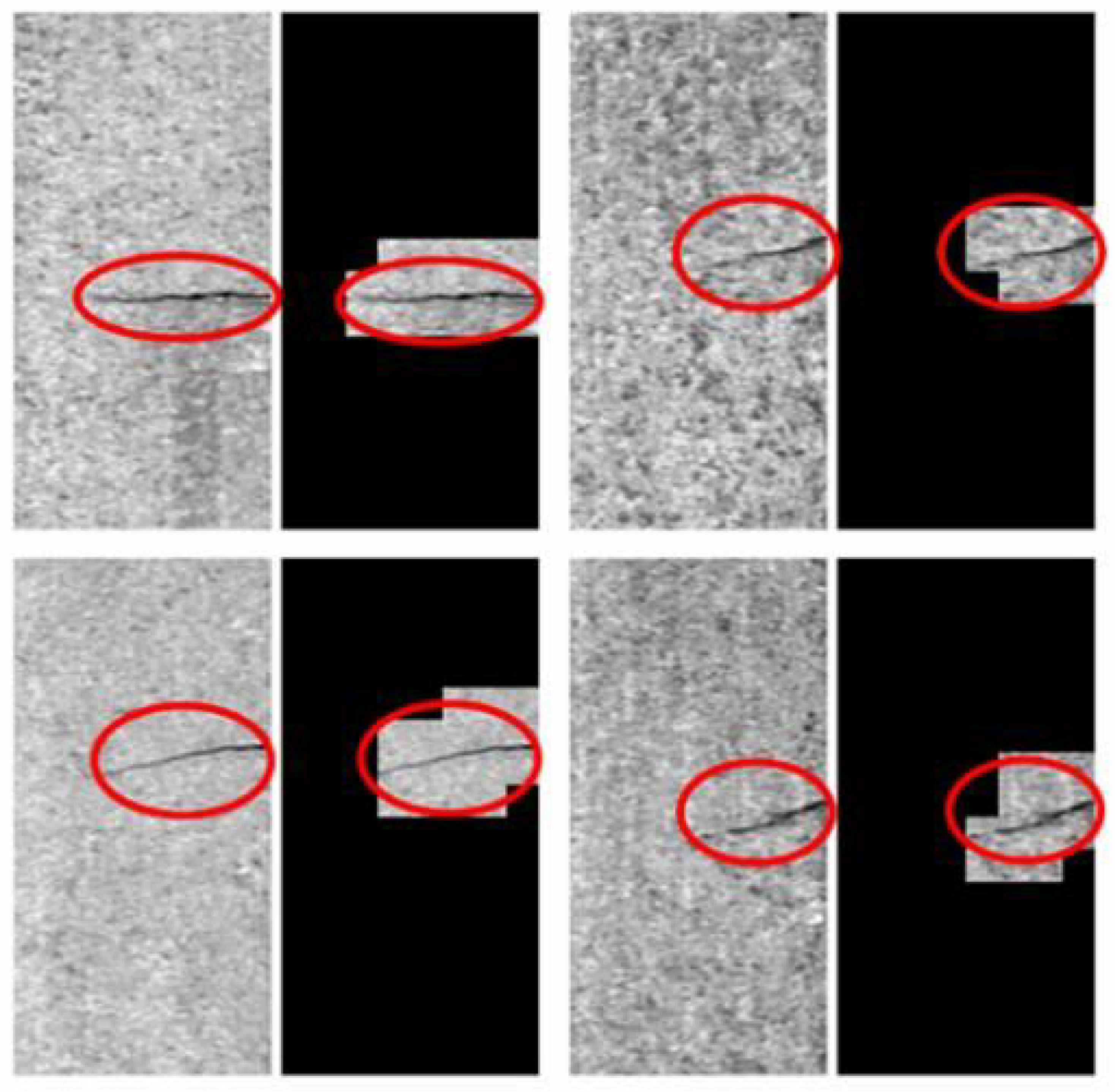
The results of the model detection are shown in the Figure 17. The non-defective area is automatically covered with black, and the defective area is manually marked with a red ellipse.
5. Conclusions
This paper proposed a defect detection method based on CNN networks and wavelet transform, which can achieve a very high level of accuracy only with a small amount of training data. The method is evaluated on the DAGM2007 dataset, micro-surface defect database and KolektorSDD dataset, and the results show that it has a good detection ability for most defective images and can locate the location of the defect. In addition, by comparing the wavelet model with the non-wavelet model, it can be found that this method has faster learning speed and detection accuracy than traditional detection methods. The method used in this paper to extract defect patches with random windows greatly saves the time of data preprocessing. There are also sliding window methods and judgment strategies that can effectively extract image features and make defect judgments. These methods can also be applied to other detection fields. In the task of small target detection, researchers can increase the proportion of the target area by extracting patches from the original image, and can also use wavelet analysis to improve the performance of the CNN model.
At the same time, this method also has some room for improvement. The detection ability of this method is not good for the image with great background texture difference. The reason is the random-window method only uses a little information from non-defective images, which is not enough for CNN training. For the images with great background texture difference, such as Class 1 and Class 4 in DAGM2007 dataset, the sliding-window method proposed in the Ref. [2] can be used to extract non-defective patches. In addition, only using the low-frequency sub-images may lose some important information for the image which is changing rapidly, such as Class 8. It can consider using high-frequency images or using high-frequency and low-frequency fusion to process training data. As for the threshold setting in the judgment strategy, we do not propose specific rules, but set them based on experience. In the follow-up research, additional experiments can be set up for different application scenarios and defect sizes to select appropriate thresholds.
Author Contributions
Conceptualization, M.D. and K.L.; methodology, K.L.; software, K.L. and D.L.; investigation, K.L. and D.L.; resources, M.D.; data curation, D.L.; writing—original draft preparation, K.L.; writing—review and editing, D.L. and J.X.; visualization, K.L. and D.L; supervision, M.D.; project administration, M.D.; funding acquisition, M.D. All authors have read and agreed to the published version of the manuscript.
Funding
This research was funded by The Key Research Projects of Henan Higher Education Institutions [grant number 18A510017]; the Henan Postdoctoral Research Project [grant number 001701004]; the Major science and technology special plan of Henan Province [grant number 201111212300]; and Henan province natural science fund item [grant number 212300410291].
Institutional Review Board Statement
Not applicable.
Informed Consent Statement
Not applicable.
Data Availability Statement
This publication is supported by multiple datasets, which are openly available. (1) DAGM 2007 dataset is openly available from The Heidelberg Collaboratory for Image Processing (DAGM 2007, https://hci.iwr.uni-heidelberg.de/content/weakly-supervised-learning-industrial-optical-inspection, accessed on 1 May 2021); (2) NEU surface defect database is openly available from Northeast University of China (NEU surface defect database, http://faculty.neu.edu.cn/songkechen/zh_CN/zdylm/263270/list/index.htm, accessed on 1 May 2021); (3) KolektorSDD dataset is openly available from Visual Cognitive Systems Laboratory, University of Ljubljana (KolektorSDD dataset, https://www.vicos.si/resources/kolektorsdd, accessed on 1 May 2021).
Conflicts of Interest
The authors declare no conflict of interest.
References
- Racki, D.; Tomazevic, D.; Skocaj, D. A Compact Convolutional Neural Network for Textured Surface Anomaly Detection. In Proceedings of the 2018 IEEE Winter Conference on Applications of Computer Vision (WACV), Lake Tahoe, NV, USA, 12–15 March 2018; pp. 1331–1339. [Google Scholar]
- Wang, T.; Chen, Y.; Qiao, M.; Snoussi, H. A fast and robust convolutional neural network-based defect detection model in product quality control. Int. J. Adv. Manuf. Technol. 2018, 94, 3465–3471. [Google Scholar] [CrossRef]
- Weimer, D.; Scholz-Reiter, B.; Shpitalni, M. Design of deep convolutional neural network architectures for automated feature extraction in industrial inspection. CIRP Ann. 2016, 65, 417–420. [Google Scholar] [CrossRef]
- Li, P.; Liang, J.; Shen, X.; Zhao, M.; Sui, L. Textile fabric defect detection based on low-rank representation. Multimed. Tools Appl. 2019, 78, 99–124. [Google Scholar] [CrossRef]
- Ma, S.; Liu, W.; You, C.; Jia, S.; Wu, Y. An improved defect detection algorithm of jean fabric based on optimized Gabor filter. J. Inf. Process. Syst. 2020, 16, 1008–1014. [Google Scholar]
- Di, L.; Long, H.; Liang, J. Fabric defect detection based on illumination correction and visual salient features. Sensors 2020, 20, 5147. [Google Scholar] [CrossRef] [PubMed]
- Zhang, H.; Ma, J.; Jing, J.; Li, P. Fabric defect detection using L0 gradient minimization and fuzzy C-means. Appl. Sci. 2019, 9, 3506. [Google Scholar] [CrossRef] [Green Version]
- Jia, L.; Zhang, J.; Chen, S.; Hou, Z. Fabric defect inspection based on lattice segmentation and lattice templates. J. Frankl. Inst. 2018, 355, 7764–7798. [Google Scholar] [CrossRef]
- Shi, K.; Wang, J.; Wang, L.; Pan, R.; Gao, W. Objective evaluation of fabric wrinkles based on 2-D Gabor transform. Fibers Polym. 2020, 21, 2138–2146. [Google Scholar] [CrossRef]
- Nguyen, V.T.; Constant, T.; Colin, F. An innovative and automated method for characterizing wood defects on trunk surfaces using high-density 3D terrestrial LiDAR data. Ann. For. Sci. 2021, 78, 1–18. [Google Scholar] [CrossRef]
- Ibrahim, M.; Headland, D.; Withayachumnankul, W.; Wang, C. Nondestructive Testing of Defects in Polymer-Matrix Composite Materials for Marine Applications Using Terahertz Waves. J. Nondestruct. Eval. 2021, 40, 1–11. [Google Scholar] [CrossRef]
- Liu, K.; Wang, H.; Chen, H.; Qu, E.; Tian, Y.; Sun, H. Steel surface defect detection using a new Haar–Weibull-variance model in unsupervised manner. IEEE Trans. Instrum. Meas. 2017, 66, 2585–2596. [Google Scholar] [CrossRef]
- Zhao, X.; He, Z.; Zhang, S.; Liang, D. A sparse-representation-based robust inspection system for hidden defects classification in casting components. Neurocomputing 2015, 153, 1–10. [Google Scholar] [CrossRef]
- Xiang, S.; Liang, D.; Kaneko, S.; Asano, H. Robust defect detection in 2D images printed on 3D micro-textured surfaces by multiple paired pixel consistency in orientation codes. IET Image Process. 2020, 14, 3373–3384. [Google Scholar] [CrossRef]
- Alzubaidi, L.; Zhang, J.; Humaidi, A.J.; Al-Dujaili, A.; Duan, Y.; Al-Shamma, O.; Santamaría, J.; Fadhel, M.A.; Al-Amidie, M.; Farhan, L. Review of deep learning: Concepts, CNN architectures, challenges, applications, future directions. J. Big Data 2021, 8, 1–74. [Google Scholar]
- Gu, J.; Wang, Z.; Kuen, J.; Ma, L.; Shahroudy, A.; Shuai, B.; Liu, T.; Wang, X.; Wang, G.; Cai, J.; et al. Recent advances in convolutional neural networks. Pattern Recognit. 2018, 77, 354–377. [Google Scholar] [CrossRef] [Green Version]
- Donahue, J.; Anne Hendricks, L.; Guadarrama, S.; Rohrbach, M.; Venugopalan, S.; Saenko, K.; Darrell, T. Long-term recurrent convolutional networks for visual recognition and description. In Proceedings of the IEEE Conference on Computer Vision and Pattern Recognition, Boston, MA, USA, 7–12 June 2015; pp. 2625–2634. [Google Scholar]
- Cha, Y.J.; Choi, W.; Büyüköztürk, O. Deep learning-based crack damage detection using convolutional neural networks. Comput.-Aided Civ. Infrastruct. Eng. 2017, 32, 361–378. [Google Scholar] [CrossRef]
- Raghavendra, U.; Fujita, H.; Bhandary, S.V.; Gudigar, A.; Tan, J.H.; Acharya, U.R. Deep convolution neural network for accurate diagnosis of glaucoma using digital fundus images. Inf. Sci. 2018, 441, 41–49. [Google Scholar] [CrossRef]
- Li, Y.; Zhang, D.; Lee, D.J. Automatic fabric defect detection with a wide-and-compact network. Neurocomputing 2019, 329, 329–338. [Google Scholar] [CrossRef]
- Zhao, Y.; Hao, K.; He, H.; Tang, X.; Wei, B. A visual long-short-term memory based integrated CNN model for fabric defect image classification. Neurocomputing 2020, 380, 259–270. [Google Scholar] [CrossRef]
- Mei, S.; Yang, H.; Yin, Z. An unsupervised-learning-based approach for automated defect inspection on textured surfaces. IEEE Trans. Instrum. Meas. 2018, 67, 1266–1277. [Google Scholar] [CrossRef]
- Fortuna-Cervantes, J.M.; Ramírez-Torres, M.T.; Martínez-Carranza, J.; Murguía-Ibarra, J.; Mejía-Carlos, M. Object detection in aerial navigation using wavelet transform and convolutional neural networks: A first approach. Program. Comput. Softw. 2020, 46, 536–547. [Google Scholar] [CrossRef]
- Cui, L.; Jiang, X.; Xu, M.; Li, W.; Lv, P.; Zhou, B. SDDNet: A fast and accurate network for surface defect detection. IEEE Trans. Instrum. Meas. 2021, 70, 1–13. [Google Scholar] [CrossRef]
- Xie, X.; Zhang, R.; Peng, L.; Peng, S. A Four-Stage Product Appearance Defect Detection Method With Small Samples. IEEE Access 2022, 10, 83740–83754. [Google Scholar] [CrossRef]
- Zhang, N.; Zhong, Y.; Dian, S. Rethinking unsupervised texture defect detection using PCA. Opt. Lasers Eng. 2023, 163, 107470. [Google Scholar] [CrossRef]
- Yan, S.; Shao, H.; Xiao, Y.; Liu, B.; Wan, J. Hybrid robust convolutional autoencoder for unsupervised anomaly detection of machine tools under noises. Robot. -Comput.-Integr. Manuf. 2023, 79, 102441. [Google Scholar] [CrossRef]
- He, Z.; Zeng, Y.; Shao, H.; Hu, H.; Xu, X. Novel motor fault detection scheme based on one-class tensor hyperdisk. Knowl.-Based Syst. 2023, 262, 110259. [Google Scholar] [CrossRef]
- Rezaei, Z.; Ebrahimpour-Komleh, H.; Eslami, B.; Chavoshinejad, R.; Totonchi, M. Adverse drug reaction detection in social media by deep learning methods. Cell J. 2020, 22, 319. [Google Scholar]
- Liu, S.; Tang, B.; Chen, Q.; Wang, X. Drug-drug interaction extraction via convolutional neural networks. Comput. Math. Methods Med. 2016, 2016, 6918381. [Google Scholar] [CrossRef] [Green Version]
- Kooi, T.; Litjens, G.; Van Ginneken, B.; Gubern-Mérida, A.; Sánchez, C.I.; Mann, R.; den Heeten, A.; Karssemeijer, N. Large scale deep learning for computer aided detection of mammographic lesions. Med. Image Anal. 2017, 35, 303–312. [Google Scholar] [CrossRef]
- Lin, T.Y.; Dollár, P.; Girshick, R.; He, K.; Hariharan, B.; Belongie, S. Feature pyramid networks for object detection. In Proceedings of the IEEE Conference on Computer Vision and Pattern Recognition, Honolulu, HI, USA, 21–26 July 2017; pp. 2117–2125. [Google Scholar]
- Quan, W.; Wang, K.; Yan, D.M.; Zhang, X. Distinguishing between natural and computer-generated images using convolutional neural networks. IEEE Trans. Inf. Forensics Secur. 2018, 13, 2772–2787. [Google Scholar] [CrossRef]
- Zhang, H.; Ji, Y.; Huang, W.; Liu, L. Sitcom-star-based clothing retrieval for video advertising: A deep learning framework. Neural Comput. Appl. 2019, 31, 7361–7380. [Google Scholar] [CrossRef]
- He, K.; Gkioxari, G.; Dollár, P.; Girshick, R. Mask r-cnn. In Proceedings of the IEEE International Conference on Computer Vision, Venice, Italy, 22–29 October 2017; pp. 2961–2969. [Google Scholar]
- Kamnitsas, K.; Ledig, C.; Newcombe, V.F.; Simpson, J.P.; Kane, A.D.; Menon, D.K.; Rueckert, D.; Glocker, B. Efficient multi-scale 3D CNN with fully connected CRF for accurate brain lesion segmentation. Med. Image Anal. 2017, 36, 61–78. [Google Scholar] [CrossRef] [PubMed]
- Liang, D.; Kang, B.; Liu, X.; Gao, P.; Tan, X.; Kaneko, S. Cross-scene foreground segmentation with supervised and unsupervised model communication. Pattern Recognit. 2021, 117, 107995. [Google Scholar] [CrossRef]
- Rhif, M.; Ben Abbes, A.; Farah, I.R.; Martínez, B.; Sang, Y. Wavelet transform application for/in non-stationary time-series analysis: A review. Appl. Sci. 2019, 9, 1345. [Google Scholar] [CrossRef] [Green Version]
- Song, K.; Yan, Y. micro-surface defect detection method for silicon steel strip based on saliency convex active contour model. Math. Probl. Eng. 2013, 2013, 429094. [Google Scholar] [CrossRef] [Green Version]
- Tabernik, D.; Šela, S.; Skvarč, J.; Skočaj, D. Segmentation-based deep-learning approach for surface-defect detection. J. Intell. Manuf. 2020, 31, 759–776. [Google Scholar] [CrossRef] [Green Version]
- He, K.; Zhang, X.; Ren, S.; Sun, J. Delving deep into rectifiers: Surpassing human-level performance on imagenet classification. In Proceedings of the IEEE International Conference on Computer Vision, Santiago, Chile, 7–13 December 2015; pp. 1026–1034. [Google Scholar]
- Jiang, X.; Scott, P.; Whitehouse, D. Wavelets and their applications for surface metrology. CIRP Ann. 2008, 57, 555–558. [Google Scholar] [CrossRef]
- Siebel, N.T.; Sommer, G. Learning defect classifiers for visual inspection images by neuro-evolution using weakly labelled training data. In Proceedings of the 2008 IEEE Congress on Evolutionary Computation (IEEE World Congress on Computational Intelligence), Hong Kong, China, 1–6 June 2008; pp. 3925–3931. [Google Scholar]
- Timm, F.; Barth, E. Non-parametric texture defect detection using Weibull features. In Image Processing: Machine Vision Applications IV; Society of Photo-Optical Instrumentation Engineers (SPIE): Bellingham, WA, USA, 2011; Volume 7877, pp. 150–161. [Google Scholar]
Figure 1.
The general process of this paper’s method. The wavelet-transformed images are extracted as defective and non-defective patches, respectively. Feed it into the network to train the model. When testing, use a sliding window to input the wavelet-transformed image into the model for judgment and decision-making.

Figure 2.
One level of wavelet decomposition. L, H, V, D represent low-frequency coefficient, horizontal high-frequency coefficient, vertical high-frequency coefficient and diagonal high-frequency coefficient.
Figure 2.
One level of wavelet decomposition. L, H, V, D represent low-frequency coefficient, horizontal high-frequency coefficient, vertical high-frequency coefficient and diagonal high-frequency coefficient.

Figure 3.
The decomposition results of the real image. The right side is the decomposed four different frequency submaps.
Figure 3.
The decomposition results of the real image. The right side is the decomposed four different frequency submaps.

Figure 4.
The process of this method in the model training phase. The original image and wavelet image are divided into patches and sent to the network for training respectively.
Figure 4.
The process of this method in the model training phase. The original image and wavelet image are divided into patches and sent to the network for training respectively.

Figure 5.
Into patches and then sent to the two models for judgment.

Figure 6.
The architecture of our CNN networks for defect detection.

Figure 7.
Label image (left) and defect image (right) in DAGM. The black spot is the center of the defect, the red rectangle is the defect patch we extracted after offset.
Figure 7.
Label image (left) and defect image (right) in DAGM. The black spot is the center of the defect, the red rectangle is the defect patch we extracted after offset.

Figure 8.
The sliding-window method in DAGM 2007. Extract all 64 × 64 patches in the image in 32 strides for prediction.
Figure 8.
The sliding-window method in DAGM 2007. Extract all 64 × 64 patches in the image in 32 strides for prediction.

Figure 9.
A defective image (right) and its probability matrix (left). The number in the box indicates the probability that the patch is non-defective.
Figure 9.
A defective image (right) and its probability matrix (left). The number in the box indicates the probability that the patch is non-defective.

Figure 10.
A non-defective image (right) and its probability matrix (left). The number in the box indicates the probability that the patch is non-defective.
Figure 10.
A non-defective image (right) and its probability matrix (left). The number in the box indicates the probability that the patch is non-defective.

Figure 11.
The image samples of 10 classes in DAGM2007 dataset. Defects are marked with red ellipses.
Figure 11.
The image samples of 10 classes in DAGM2007 dataset. Defects are marked with red ellipses.

Figure 12.
The image samples of two classes in the micro-surface defect database. Defects are marked with red ellipses.
Figure 12.
The image samples of two classes in the micro-surface defect database. Defects are marked with red ellipses.

Figure 13.
The image samples in the KolektorSDD dataset. Defects are marked with red ellipses.

Figure 14.
The examples of detection results in the DAGM2007 dataset. The red ellipse marks the location of the defect. The left image is the image to be detected, and the right image is the detection result. Our model judges that areas without defects are covered with black images.
Figure 14.
The examples of detection results in the DAGM2007 dataset. The red ellipse marks the location of the defect. The left image is the image to be detected, and the right image is the detection result. Our model judges that areas without defects are covered with black images.

Figure 15.
The accuracy curve and loss curve of the wavelet model and non-wavelet model.

Figure 16.
The examples of detection results in a micro-surface defect database. The red ellipse marks the location of the defect. The left image is the image to be detected, and the right image is the detection result. Our model judges that areas without defects are covered with black images.
Figure 16.
The examples of detection results in a micro-surface defect database. The red ellipse marks the location of the defect. The left image is the image to be detected, and the right image is the detection result. Our model judges that areas without defects are covered with black images.

Figure 17.
The examples of detection results in the KolektorSDD dataset. The red ellipse marks the location of the defect. The left image is the image to be detected, and the right image is the detection result. Our model judges that areas without defects are covered with black images.
Figure 17.
The examples of detection results in the KolektorSDD dataset. The red ellipse marks the location of the defect. The left image is the image to be detected, and the right image is the detection result. Our model judges that areas without defects are covered with black images.


Table 1.
The image distribution of each class.
| Class | Class2 | Class3 | Class6 | Class7 | Class8 | Class9 | Class10 | Total |
|---|---|---|---|---|---|---|---|---|
| Train(P/N) 1 | 120/970 | 100/800 | 100/800 | 200/1800 | 200/800 | 200/1800 | 200/1800 | 1120/9770 |
| Test(P/N) 1 | 30/30 | 50/200 | 50/200 | 100/200 | 100/200 | 100/200 | 100/200 | 530/1230 |
1 Here “P” indicates defective images, “N” indicates non-defective images.
Table 2.
The number of training patches of each class in the wavelet model.
| Class | Class2 | Class3 | Class6 | Class7 | Class8 | Class9 | Class10 | Total |
|---|---|---|---|---|---|---|---|---|
| Defective patches | 1503 | 1758 | 2370 | 3690 | 2814 | 2930 | 4504 | 19,589 |
| Non-defective patches | 3880 | 3200 | 2400 | 7200 | 7200 | 6000 | 5400 | 35,280 |
Table 3.
The results of our methods in the DAGM2007 dataset and the comparison of others. Here, TPR and TNR are recorded by adjusting the threshold of the judgment strategy to make the acc maximum.
Table 3.
The results of our methods in the DAGM2007 dataset and the comparison of others. Here, TPR and TNR are recorded by adjusting the threshold of the judgment strategy to make the acc maximum.
| Class | Our Non-Wavelet Model | Our Wavelet Mode | Xie’s Model [25] | Racki’s CNN [1] | Wang’s CNN [2] | Weimer’s CNN [3] | Statistical Features [42] | SIFT and ANN [43] | Weibull [44] | Zhang’s Model [26] |
|---|---|---|---|---|---|---|---|---|---|---|
| TPR (%) | ||||||||||
| 2 | 95.8 | 97.5 | 100 | 100 | 100 | 100 | 94.3 | 95.7 | - * | 92.5 |
| 3 | 87.0 | 100 | 100 | 100 | 100 | 95.5 | 99.5 | 98.5 | 99.8 | 89.6 |
| 6 | 100 | 99 | 100 | 100 | 100 | 100 | 100 | 99.8 | 94.9 | 93.8 |
| 7 | 66.5 | 97.5 | 100 | 100 | - | - | - | - | - | 95.9 |
| 8 | 100 | 96.5 | 100 | 100 | - | - | - | - | - | 95.9 |
| 9 | 74 | 99.5 | 100 | 100 | - | - | - | - | - | - |
| 10 | 51 | 92 | 100 | 100 | - | - | - | - | - | - |
| TNR (%) | ||||||||||
| 2 | 97.5 | 99.4 | 100 | 99.8 | 100 | 97.3 | 80 | 91.3 | - | - |
| 3 | 98.8 | 99 | 100 | 96.3 | 100 | 100 | 100 | 100 | 100 | - |
| 6 | 100 | 99.9 | 100 | 100 | 100 | 99.5 | 96.1 | 100 | 100 | - |
| 7 | 100 | 99.5 | 100 | 100 | - | - | - | - | - | - |
| 8 | 100 | 98.9 | 100 | 100 | - | - | - | - | - | - |
| 9 | 95.9 | 100 | 100 | 99.9 | - | - | - | - | - | - |
| 10 | 99.9 | 99.8 | 100 | 100 | - | - | - | - | - | - |
| AVEACC (%) | ||||||||||
| 96.1 | 99.3 | 100 | 99.7 | 99.8 | 99.2 | 95.9 | 98.2 | 97.1 | - |
Table 4.
The number of pixels in each training set between our method and others.
| Class | Our Wavelet Model | Racki’s CNN [1] | Wang’s CNN [2] | Weimer’S CNN [3] |
|---|---|---|---|---|
| Class1–6 | 20,631,552 px | 209,190,912 px | 867,631,104 px | 221,729,792 px |
| (5037 × 64 × 64) * | (798 × 512 × 512) | (52,956 × 128 × 128) | (216,533 × 32 × 32) | |
| Class7–10 | 40,710,144 px | 419,430,400 px | - | - |
| (9939 × 64 × 64) | (1600 × 512 × 512) | - | - | |
| Ratio | 1 | 10.24 | 42.05 | 10.75 |
| AVEACC (%) | 99.3 | 99.7 | 99.8 | 99.2 |
* “5037 × 64 × 64” means in the first six classes of training data, there are about 5037 patches (64 × 64 pixels) in
each class.
Table 5.
The performance criteria of detecting SDI and SDPI.
| Class | TP | FP | FN | Recall (%) | Precession (%) |
|---|---|---|---|---|---|
| SDI * | 24 | 0 | 2 | 92.3 | 100 |
| SDPI * | 24 | 1 | 1 | 96 | 96 |
* SDI and SPDI refer to the pot-defect image and Steel-pit-defect image in this dataset, respectively.
Table 6.
The performance criteria of detecting the KolektorSDD dataset.
| TP | FP | FN | Recall (%) | Precession (%) |
|---|---|---|---|---|
| 16 | 0 | 4 | 80 | 100 |
Disclaimer/Publisher’s Note: The statements, opinions and data contained in all publications are solely those of the individual author(s) and contributor(s) and not of MDPI and/or the editor(s). MDPI and/or the editor(s) disclaim responsibility for any injury to people or property resulting from any ideas, methods, instructions or products referred to in the content. |
© 2023 by the authors. Licensee MDPI, Basel, Switzerland. This article is an open access article distributed under the terms and conditions of the Creative Commons Attribution (CC BY) license (https://creativecommons.org/licenses/by/4.0/).
Share and Cite
MDPI and ACS Style
Dong, M.; Li, D.; Li, K.; Xu, J. TSDNet: A New Multiscale Texture Surface Defect Detection Model. Appl. Sci. 2023, 13, 3289. https://doi.org/10.3390/app13053289
AMA Style
Dong M, Li D, Li K, Xu J. TSDNet: A New Multiscale Texture Surface Defect Detection Model. Applied Sciences. 2023; 13(5):3289. https://doi.org/10.3390/app13053289
Chicago/Turabian StyleDong, Min, Dezhen Li, Kaixiang Li, and Junpeng Xu. 2023. "TSDNet: A New Multiscale Texture Surface Defect Detection Model" Applied Sciences 13, no. 5: 3289. https://doi.org/10.3390/app13053289
Note that from the first issue of 2016, this journal uses article numbers instead of page numbers. See further details here.