
Improved Stress Classification Using Automatic Feature Selection from Heart Rate and Respiratory Rate Time Signals


1
Smart Sensor Lab, Lambe Institute of Translational Research, College of Medicine, Nursing Health Sciences, University of Galway, H91 TK33 Galway, Ireland
2
Electrical and Electronic Engineering, University of Galway, H91 TK33 Galway, Ireland
3
CÚRAM Center for Research in Medical Devices, H91 W2TY Galway, Ireland
4
Centre for Systems Modelling and Quantitative Biomedicine (SMQB), University of Birmingham, Birmingham B15 2TT, UK
*
Authors to whom correspondence should be addressed.
Appl. Sci. 2023, 13(5), 2950; https://doi.org/10.3390/app13052950
Submission received: 29 January 2023
/
Revised: 20 February 2023
/
Accepted: 23 February 2023
/
Published: 24 February 2023
(This article belongs to the Special Issue Medical Imaging Using Machine Learning and Deep Learning)
Abstract
:Time-series features are the characteristics of data periodically collected over time. The calculation of time-series features helps in understanding the underlying patterns and structure of the data, as well as in visualizing the data. The manual calculation and selection of time-series feature from a large temporal dataset are time-consuming. It requires researchers to consider several signal-processing algorithms and time-series analysis methods to identify and extract meaningful features from the given time-series data. These features are the core of a machine learning-based predictive model and are designed to describe the informative characteristics of the time-series signal. For accurate stress monitoring, it is essential that these features are not only informative but also well-distinguishable and interpretable by the classification models. Recently, a lot of work has been carried out on automating the extraction and selection of times-series features. In this paper, a correlation-based time-series feature selection algorithm is proposed and evaluated on the stress-predict dataset. The algorithm calculates a list of 1578 features of heart rate and respiratory rate signals (combined) using the tsfresh library. These features are then shortlisted to the more specific time-series features using Principal Component Analysis (PCA) and Pearson, Kendall, and Spearman correlation ranking techniques. A comparative study of conventional statistical features (like, mean, standard deviation, median, and mean absolute deviation) versus correlation-based selected features is performed using linear (logistic regression), ensemble (random forest), and clustering (k-nearest neighbours) predictive models. The correlation-based selected features achieved higher classification performance with an accuracy of 98.6% as compared to the conventional statistical feature’s 67.4%. The outcome of the proposed study suggests that it is vital to have better analytical features rather than conventional statistical features for accurate stress classification.
1. Introduction
In recent years, sensor technologies have been significantly developed to help generate large data at a relatively low cost [1]. The fields of the Internet of Things (IoT) [2], precision medicine [3], and industry 4.0 [4] produce advanced, large temporally annotated data. The analysis of this large temporal data, as it is, is a dilemma for researchers and data scientists. Thus, it encourages the reduction of large time-series data into smaller series and captures ample characteristics of primary data to improve the analysis. The resulting time series is the basis of machine learning applications, such as analysis of heartbeat [5] and respiratory rate [6], identification of high-risk patients who are at increased risk of infection [7], optimization of a production line [8], or incident detection over cloud [9]. The reduction of large data to feature-based representation is crucial, as the implementation of the machine learning algorithm is straightforward, but the selection of well-discriminating features is a challenging task [10].
Time-series data are a sequence of measurements/observations sequentially taken in time [11]. In the context of stress, time-series data are referred to as a collection of data points over a period that measures the psychological or physiological responses of an individual to any applied stressor. These data points are collected at regular intervals (per second, per minute, or hour) and include measurements of respiratory rate, heart rate, cortisol levels, blood pressure, or a self-reporting stress level. The time-series data are analysed to understand the stress patterns over time, which provides better insights into how an individual’s stress levels change in response to different stressors and interventions. The learnings can be then used to develop algorithms or classification models to predict individuals’ stress conditions based on their response to stress.
Considering as a set of time-series data, where . To use set as an input to supervised or unsupervised classification algorithms, each time-series must be mapped to a well-defined feature vector with dimensions () [12]. The most efficient and effective way of feature extraction is to characterize the time-series data into a distribution of data, stationarity, correlation properties, entropy, and non-linear time-series analysis [13,14,15,16]. The extraction of only significant features is vital for both regression and classification tasks, as the irrelevant features will weaken the algorithm’s ability to generalize beyond the training set and causes overfitting [17].
Stress can be defined as a disturbance in the homeostatic balance of the body. Activation of the stress response triggers the sympathetic nervous system and inhibition of the parasympathetic system, which causes the release of stress hormones. These hormones change the heart rate, blood supply to muscles, and respiratory rate and increase cognitive activities to cope with stressors. These stress-specific responses are commonly used to quantitively assess or monitor stress [18,19,20,21]. The statistical analysis of different physiological parameters including muscle activation, skin conductance, skin temperature, brain signals, respiratory rate, heart rate, and their variations, and classification analysis leading to shortlisting of respiratory rate and heart rate was illustrated in [22] and also used by [23,24].
1.1. Related Work
Many existing stress classification studies have used trivial feature extraction and selection methods. These studies use either raw data (data collected through the sensors) [25,26] or common features of the collected data [27,28,29], such as rate of change, mean, standard deviation, variance, mean absolute deviation, and skewness. This set of features does not fully describe the characteristics of the dataset and is also unable to be generalised to another time-series dataset. This is because the underlying patterns and characteristics of a particular dataset are specific to itself and cannot be applied to another dataset. Furthermore, the abovementioned features are also affected by the conditions under which data are collected and the pre-processing steps performed on them.
Christ et al. [12] proposed tsfresh, a machine-learning time-series feature extraction library that has been used in several studies. The library uses a method called AutoTS (Automatic Time-Series Feature Extraction) and is based on some pre-defined feature estimation algorithms. It estimates the trends, seasonality, periodicity, and volatility of the time-series data and applies the feature selection method to select the most relevant features for further modelling or analysis. Several studies have used the tsfresh library for feature engineering. Ouyang et al. [30] used the tsfresh feature extraction library to detect anomalous power consumption by users. They extracted 794 features that were used as input to the supervised binary classification (to detect abnormalities). However, the authors did not perform any feature selection, which makes their approach computationally expensive and not feasible to be implemented in real-time. Zhang et al. [31] proposed unsupervised anomaly detection using DBSCAN and feature engineering. The authors used the tsfresh library in their feature engineering process. They performed features selected based on Maximum-Relevance Minimum-redundancy and variance technique along with Maximal Information Coefficient. However, the proposed approach works best with historical data (as the calculation of relevance, redundancy, and information coefficients is performed on complete data) and cannot be applied to real-world or streaming data. In the field of healthcare, Liu et al. [32] recommended a solution for the classification of flawed sensors using tsfresh feature extraction and selection. The algorithm automatically calculated and selected features using univariate hypothesis tests with a controlled false discovery rate [33]. The selected features were fed into a Long-Short-Term Memory (LSTM) model for classification. However, the extracted features were still over hundreds of features.
Thus, further research is required to obtain a well-generalizable feature engineering algorithm that can calculate and provide well-distinguishable features from large time-series data for an accurate and efficient classification (monitoring) system.
1.2. Motivation and Contribution
For extremely large data, the current automated feature estimation algorithms are not able to capture sufficient valuable information about the feature dynamics [34]. The research aims of this study are to implement and explore the efficacy of the heart rate and respiratory rate signal-based (time-series) features extraction algorithm for accurate stress classification, using a stress-predict dataset [35]. The study also determines the best (well-distinguishable) time-series feature from respiratory and heart rate signals for accurate stress monitoring. The algorithm calculates several time-series features using the tsfresh library and then performs anomaly detection (leading to feature reduction) using principal component analysis (PCA) and correlation co-efficient analysis (Pearson, Spearman, and Kendall) to shortlist the most discriminative features.
For validation of the proposed method, a combination of different extracted features is fed into supervised linear, ensemble, and clustering classifiers. The proposed method of time-series features estimation/extraction and feature selection, due to its fast computation and selection of well-distinguishable stress features, can potentially be deployed on photoplethysmography (PPG) sensor-based watches and can detect the anomalies (stress) in real-time.
The rest of the paper is organised as follows. Section 2 discusses the stress-predict dataset and methods implemented for time-series features extraction and selection; Section 3 reports the detailed analysis and results of supervised machine learning classification and provides discussion around the results; Section 4 concludes the paper and provides future direction towards the development of the reliable stress-monitoring device.
2. Material and Methods
2.1. Stress-Predict Dataset
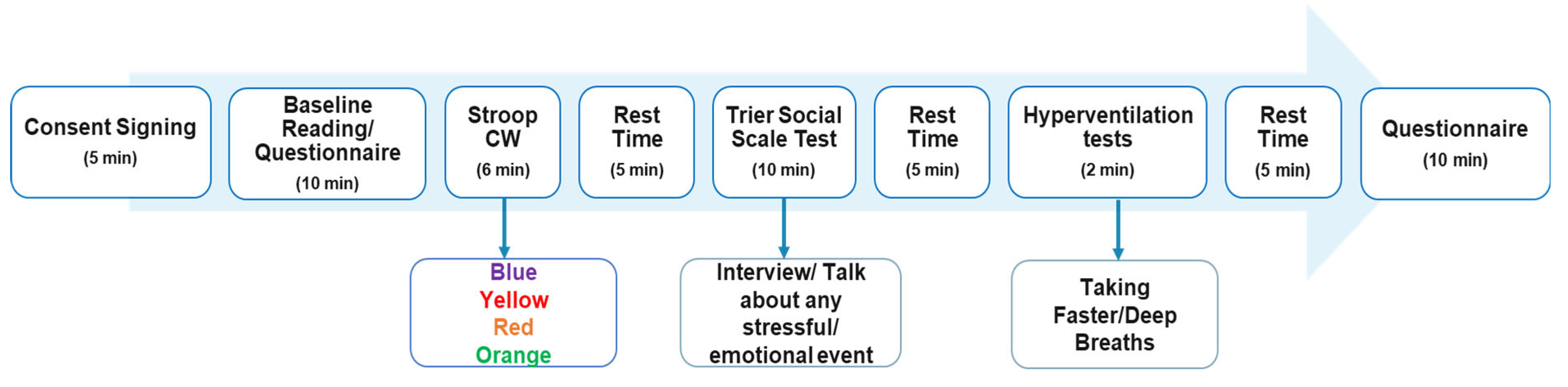
The stress-predict dataset consisted of a BVP signal, inter-beat-intervals, heart rate, respiratory rate, and accelerometer data collected from 35 healthy volunteers who performed three stress-inducing tasks (i.e., Stroop colour word test, an interview session, and hyperventilation period) with baseline/normal period. Empatica E4 was used to collect all the information, while the overall study lasted for 60 min per participant [35]. A brief introduction to the dataset is presented as follows.
The study was designed to be a cross-sectional study that collected data on exposure and outcomes in a short time window, in a controlled laboratory setting. The study aimed to understand the behaviour, attitudes, and prevalence to estimate health needs.
2.1.1. Study Methodology and Protocol
The study took 60 min per participant and was completely non-invasive. The protocol followed is illustrated in Figure 1, while Table 1 enlists the inclusion and exclusion criteria for the study. The data were only collected from healthy volunteers, who could quickly recover from the stress state induced by the questionnaire. The age bracket selected for the volunteers was 18 to 75 years old. Furthermore, the volunteers needed to be able to speak English (as all communication and consent forms were in English) and agreed (gave consent) to participate in the study. The exclusion criteria included people who did not consent to participate, unhealthy individuals (as stress might lead them to any acute event), breastfeeding mothers and pregnant women (as stress might harm them and/or their child), and colour-blind people (as one of the stressors was a Colour-Word Stroop test, where the colour name is selected based on the colour seen on the screen).
The protocol and clinical study were approved by the Clinical Research Ethics Committee, Merlin Park Hospital, Galway, Ireland, as: “Stress levels monitoring using sensor-derived signals from non-invasive wearable devices and dataset development (Ref: C.A. 2731)”. For sample size calculation, authors followed sensitivity analysis outcomes reported in [22]. The data from all the participants were collected in the daytime (the precise time for data collection was chosen by the participants). Moreover, participants arriving at the study site were asked to sit and relax for 5 min to bring their heart rate and respiratory rate to normal levels.
2.1.2. Data Acquisition
The study used an Empatica E4 wrist-worn watch to measure physiological changes based on the PPG signal. Labelling of the data was performed by using tags generated by pressing the button on the watch at the start and end of each task.
The data sheet of the stress-predict dataset illustrates that the data were gathered from 10 males (average age: 31 ± 5.8 years) and 25 females (average age: 33 ± 10.7 years). The majority of the subjects for the data collection were females. One of the reasons for this is that future studies will be based on evaluating the proposed algorithm for breast cancer patients. As breast cancer is mostly a prevalent disease among females, therefore, the majority of the subjects for data collection were females.
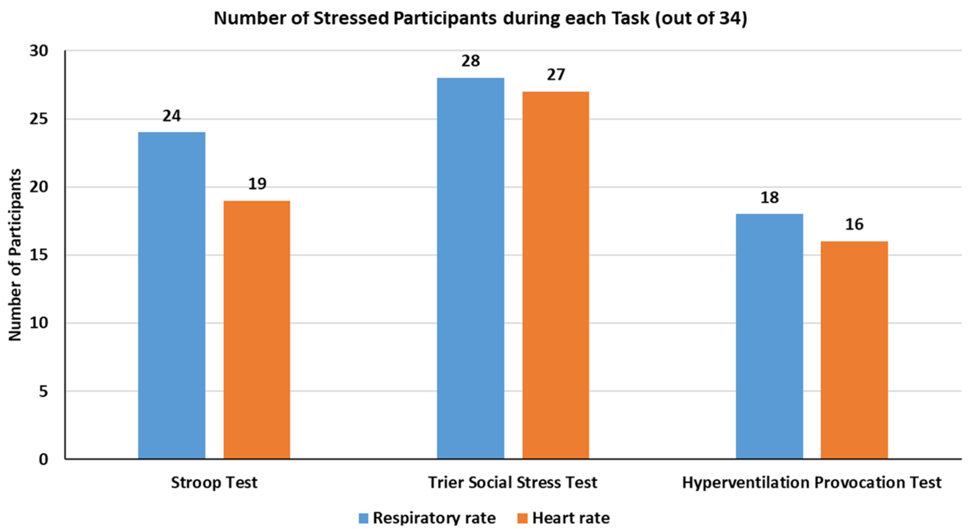
Table 2 summarizes the number of data entries per participant for each signal recorded. The total recording time reported was approximately around 50 min. The heart rate and respiratory rate signals were generated using 10 s windows (averaged over 10 s) with a window step (slide) of 1 s. Figure 2 shows the number of participants who reported higher stress levels during the study based on respiratory and heart rate signal gradients. The analysis of inter- and intra-personal variability within the data is provided in [35]. The population-based analysis using a linear mixer model showed that participants experienced a 5.05 bpm higher change in HR per hour compared to during a normal state (95% CI 4.36, 5.74 bpm/hour; p < 0.001). For respiratory rate, the participants experienced a decrease in breathing rate by 1.11 breaths per minute, a change in respiratory rate per hour compared to during a normal state. The drop in the RR can be related to sighs (deep breaths when under stress). Alternatively, individual participant analysis showed that 79.4% of participants had heart rate values outside of their normal (reference) range during stress, while the respiratory rate of over 82% of participants changed to outside their normal respiratory rate while under stress.
2.2. Feature Extraction and Selection
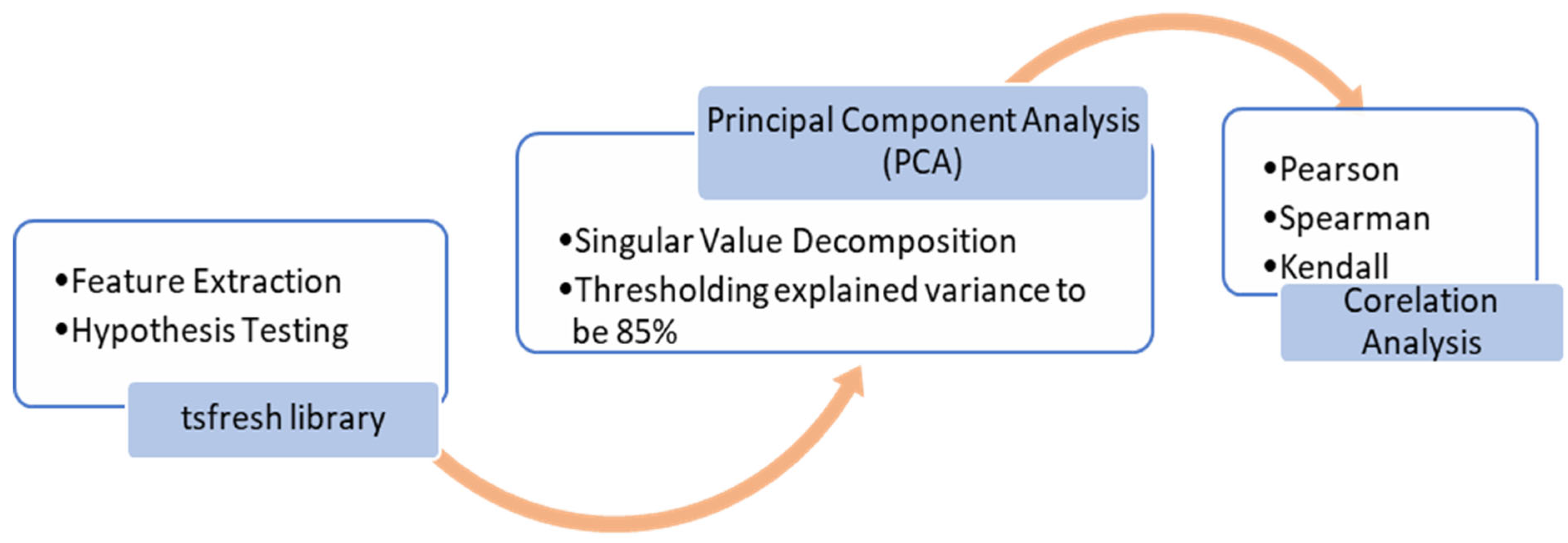
Recently, efforts have been made to automate time-series feature extraction methods and calculate hundreds of different features [17,36]. However, these high dimensional features lead to challenges when calculating, predicting, storing, and even understanding the correlation of data with the target/outcome [37]. A common technique used for time-series feature extraction is windowing (data are divided into smaller windows and features are extracted for each window) [38]. Features such as mean can reduce signal noise, but averages the overall signal. On the contrary, some features such as maximum can be unduly affected by noise [36]. As automated feature extraction has limitations and motivates the need for a systematic process of feature selection along with feature extraction [12], this study implements a three-stage feature extraction and selection algorithm. Each stage is explained in the following subsection, illustrated in Figure 3.
2.2.1. tsfresh Library
Features were extracted using the Python library tsfresh [39]. The library is composed of a combination of 63 time-series characterization techniques. The library calculates 794 features (based on estimating trends, seasonality, and periodicity of the data) by default and shortlists the features based on automatically configured hypothesis tests [12]. The library uses standard APIs for time-series (pandas) and machine learning (scikit-learn) packages and provides exploratory analyses. A list of the calculated features and their respective runtimes is documented in [40].
2.2.2. Principal Component Analysis (PCA)
Principal component analysis (PCA) is a statistical method that is generally used to reduce the dimensionality of high-dimensional data [41]. PCA projects the multidimensional data into a new reduced linear coordinate system using Singular Value Decomposition (SVD). The coordinates of this system represent the largest aggregate of variance within a time-series dataset and are useful for better visualization and interpretation of complex multivariable data. The dimensionality reduction helps to observe trends, clusters, and outliers within data [42,43]. In the proposed study, principal components were selected based on the explained variance of the features. All features that had explained the proportion of variance exceeding 85% were selected for further analysis.
2.2.3. Correlation Analysis
The tsfresh and PCA eliminate calculated time-series features based on hypothesis testing (feature vs target significance) and explain the variance of the features. For a classification problem, it is vital to remove the highly correlated features as they can introduce bias in the training of the model, make the model computationally expensive (as the model learns the same information after skimming several different correlated features), reduce the precision of coefficient estimation, and affect the interpretability [44,45]. Thus, this study recommends correlation analysis to ensure the selection of weakly correlated, well-distinguishable features for an accurate, precise, and easily interpretable classification model. The three commonly used methods for correlation analysis are described below.
Pearson Correlation Coefficient
The Pearson correlation coefficient [46,47] is a statistical test that measures the ratio between the covariance of two features and their standard deviations. The coefficients show the magnitude of correlation/association and the direction (positive or negative) of the relationship. The value of the Pearson coefficient varies between −1 and +1, and is calculated as:
In Equation (1), is the Pearson correlation coefficient, and is the the value of two features, while and is the mean value of the and features.
Spearman Ranking Correlation Coefficient
The Spearman ranking correlation [48,49] is a statistical test that measures how closely two features fluctuate. The features are ranked based on their similarity and dissimilarity, and then correlation/association between the features is calculated using the following equation (Equation (2)):
where is the Spearman coefficient, is the difference between each feature rank, while is the total number of observations. The value of the Spearman coefficient also varies between −1 to +1.
Kendall Ranking Correlation Coefficient
Kendall ranking correlation [50,51] analysis is a statistical method of measuring the rank association of the two measured features. The correlation is determined based on the concordance and discordance values, and is determined as:
In Equation (3), is the Kendall coefficient, is the number of concordant values (i.e., and have the same sign), is the number of discordant values (i.e., and have an opposite sign), while is the total number of observations and , are the two features. The correlation coefficient calculated using the Kendall method could vary between −1 and +1.
2.3. Machine Learning Classification
Machine learning classifiers are computer-based models that can learn and adapt without any explicit instructions using statistics and algorithms rules. The machine learning classifier must be generalizable (measurement of the trained classifier’s ability to accurately classify the unseen data). A generalised model presents the best trade-off between bias and variance and provides the best prediction performance [53,54]. In this study, three commonly used supervised machine learning classifiers, i.e., logistic regression classifier, random forest classifier, and k-nearest neighbour classifier, are implemented. Each of these classifiers is representative of their classification categories (linear, ensemble, and clustering). The selection of these classifiers is based on their simplicity, efficiency, interpretability, robustness, and regularization when used for binary classification of categorical-natured data; in this case, stress versus non-stress conditions.
2.3.1. Data Split for Training and Testing
For classification analysis, the dataset needs to be divided into test and train sets. Splitting the dataset helps to evaluate the performance of the model on unseen data. The training set will allow the model to fit and adjust the weights of the model while the test set evaluates the model performance on the new dataset, prevent overfitting, and ensures the model’s generalizability. As the stress-predict dataset is imbalanced (more baseline readings than stress readings), the standard classification techniques focus on minimizing the error rate and ignore the minority class. Furthermore, the random split of the imbalanced data might have negligible or no data from the minority class, thus resulting in biased classification results. The solution to the problem is the use of a stratified k-fold classification split. Stratified sampling ensures that splitting is randomly performed and that the same imbalance class distribution is maintained for each subset (fold). Thus, to obtain an unbiased model performance, stratified 10-fold cross-validation was implemented.
2.3.2. Performance Validation Methods
The performance of the classifier is validated based on accuracy, standard deviation, precision, recall, f1-score, sensitivity, and specificity. These metrics are described in [55,56,57]. Accuracy is defined as the ability of the classifier to correctly predict the label of the data point within the test dataset. Precision is the classifier’s ability to predict a data point belonging to a certain class, while Recall is the classifier’s ability to identify all the data points within a certain class. The F1-score is a combination of precision and recall using a harmonic mean. The Sensitivity of a classifier is a metric that shows its ability to predict true positives within each class, and Specificity is the evaluation metric that measures the ability to predict true negatives with each class. Table 4 shows the confusion matrix used to determine true positive and true negative readings.
3. Results and Discussions
Figure 3 demonstrates the steps of feature extraction and shortlisting. For the stress-predict dataset, the tsfresh library calculates 1578 trends, seasonality, periodicity, and volatility-based features for heart rate (789) and respiratory rate (789) signals, combined. The hypothesis test (p-value) is performed within the library to check the independence between each feature and label (target variable) and selects 314 features out of 1578 features. For further dimensionality reduction, PCA using singular value decomposition (SVD) was performed. For comparison, PCA resulted in 37 features when implemented on a full feature set (1578), while selecting only 19 features with the feature set obtained after Kruskal-Wallis’s hypothesis test (314). As the selected features might still have correlated features, a correlation analysis was performed using Pearson, Kendall, and Spearman methods to determine the most specific features of heart rate and respiratory rate signals to accurately distinguish stress conditions.
3.1. Correlation Analysis
Table 5 summarises the number of calculated and selected features at each stage.
Correlation analysis shortlisted similar features, even though they were provided with a different number of features (Filtered, PCA on full, and PCA on filtered features). The selected features are tabulated and described in Table 6 and detailed in [58].
It can be noted that all three (Pearson, Kendall, and Spearman) correlation analysis methods resulted in shortlisting the number of peaks within the time series, specifically for respiratory rate, as the most well-distinguishable feature for accurate stress monitoring. This finding is perfectly correlated with the previously published literature [6,22,35] and is true, as the breathing pattern is supposed to significantly vary during stress conditions when compared to baseline/normal conditions.
As most of the shortlisted features belong to the respiratory rate signal, this study also performed a univariable time-series correlation analysis on the heart rate signal (only feeding the heart rate signal along with labels to the algorithm) to determine the most specific heart rate-related features. The Pearson, Kendall, and Spearman correlation analysis method determined that the ‘number_cwt_peaks_n_5′ feature (number of peaks that are at enough of a width scale (here, five) and have high signal-to-noise ratio) is the most specific feature of heart rate signal to distinguish stress from the baseline readings.
3.2. Machine Learning Classifications
For classification analysis, the commonly used statistical features (mean, standard deviation, median, median absolute deviation) and the shortlisted features after correlation analysis were used to train supervised machine learning classifiers. For supervised learning, logistic regression, random forest, and K-nearest neighbours (KNN) were selected from linear, ensemble, and clustering models, respectively. The results of each classification analysis are reported as follows.
3.2.1. Standard Statistical Features
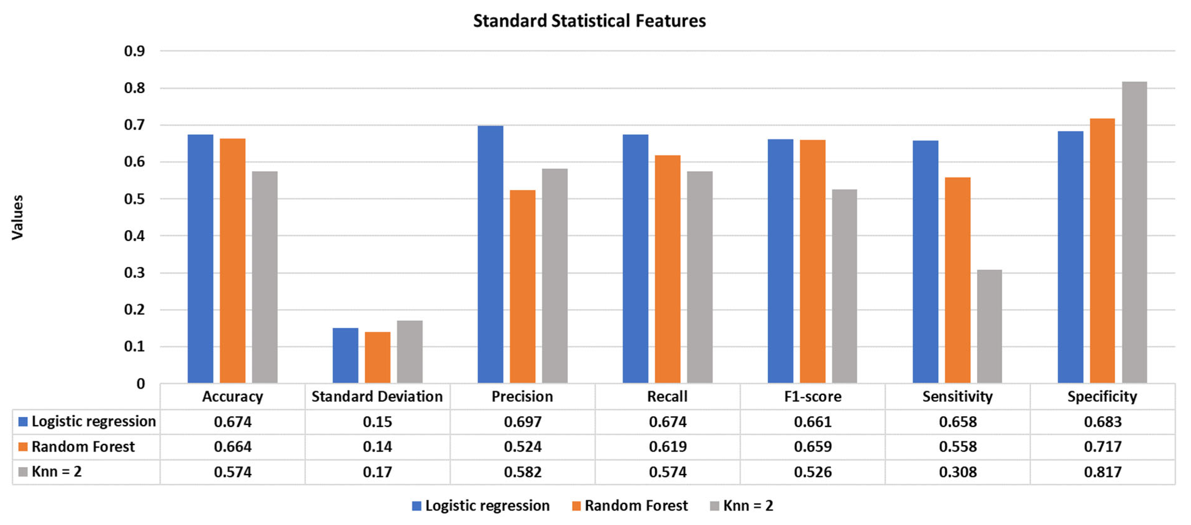
Using standard statistical features, the highest classification performance was achieved using the logistic regression model with an accuracy of 67.4%. Figure 4 illustrates the accuracy, standard deviation, precision, recall, f1-score, specificity, and sensitivity of the reported classifiers.
3.2.2. Selected Features after Correlation Analysis
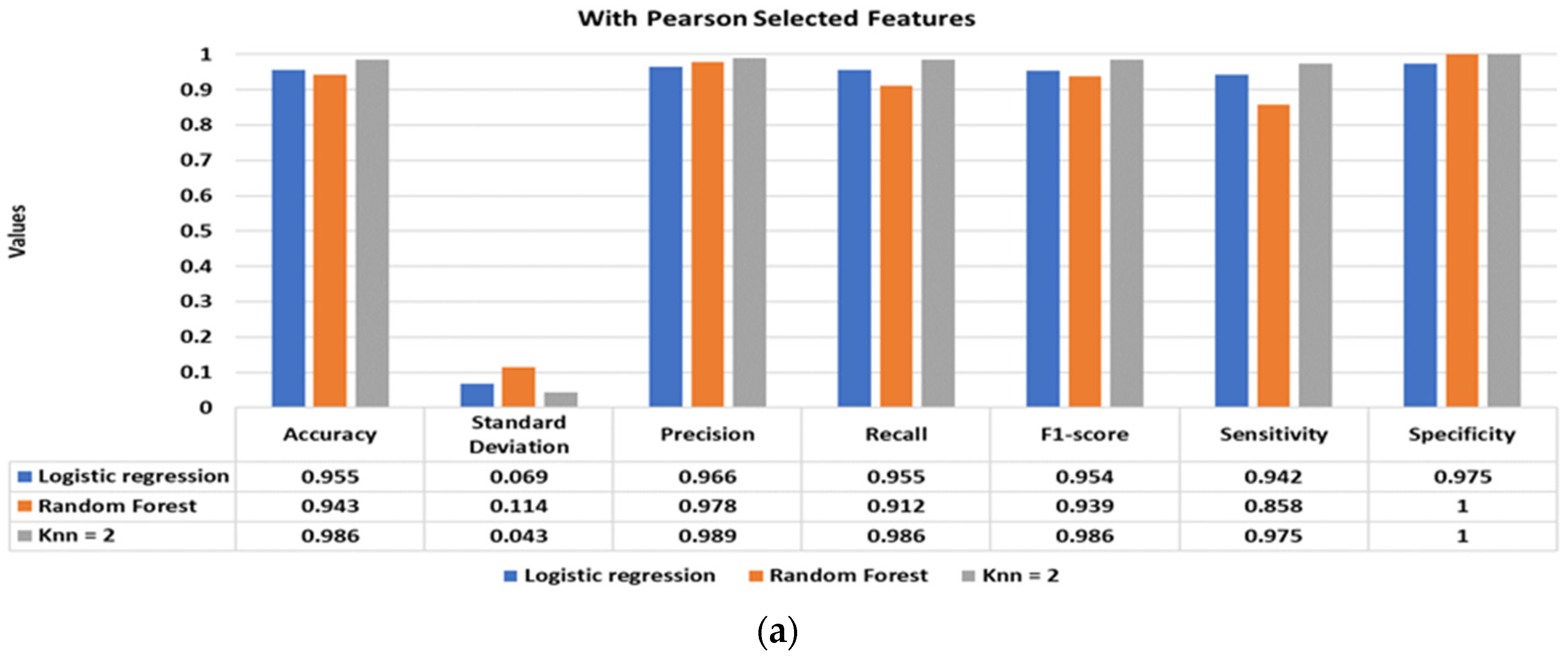
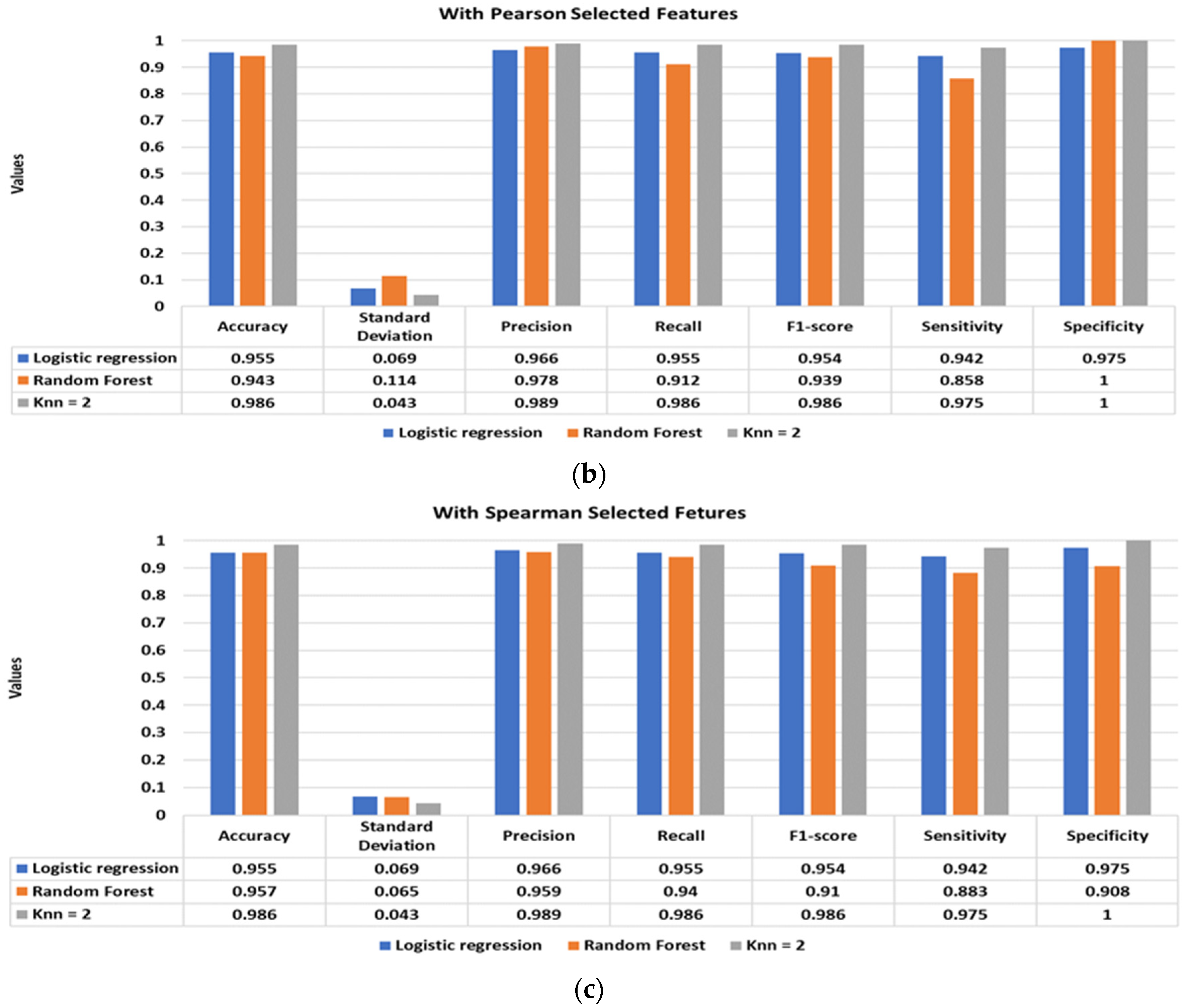
Figure 5 illustrates the classification performance of the supervised classifiers using Pearson (Figure 5a), Kendall (Figure 5b), and Spearman (Figure 5c) selected features. The inclusion of the shortlisted features with the standard statistical features significantly improves the classification performance. The best classification performance is achieved using Pearson and Spearman-based features, with a classification accuracy of 98.6% using the KNN classifier. Moreover, the other performance matrices, such as standard deviation, precision, recall, f1-score, sensitivity, and specificity, of the models have also drastically improved, achieving values well above 95%.
3.3. Summary
Automated feature extraction and selection do help in the development of a highly accurate classification model that could be generalizable to new, unseen time-series data. Time-series feature engineering is a substantial component of machine learning classification analytics. The irrelevant features within the training dataset make the model overfitted to a specific dataset and are not well generalizable. Thus, systematic time-series feature engineering allows automation of the overall classification process and a reduction in the difficulties faced during manual feature estimation and selection.
In the context of stress classification, feature engineering plays a vital role in improving classification performance. The careful selection and estimation of the time-series features do help in achieving higher classification accuracy with better interpretability of the classifier’s decision and achieved results. The dimensionality reduction also helps the predictive model to be computationally efficient, especially if required to run on resource-constrained devices.
A comparison of the proposed correlation-based feature extraction algorithm with other existing methods is shown below (Table 7).
4. Conclusions
In this study, three-fold feature extraction and selection steps are proposed. In the first step, the tsfresh library is used to calculate 1578 time-series features of heart rate and respiratory rate (789 features each) signals, which are then shortlisted to 314 features after the hypothesis test. In the second stage, PCA is applied to further reduce the feature dimensions from 314 to only 19 feature components. To detect and eliminate the most correlated features with the estimated feature list, a correlation analysis (with a threshold coefficient value of ±0.4) is performed using three different methods. The Pearson, Kendall, and Spearman correlation analysis determined the count of peaks within the respiratory rate reading to be the best and well-distinguishable feature among all other heart rate and respiratory rate-related features. For the univariate (heart rate signal) analysis, the number of CWT peaks was the most specific feature to distinguish the stress state from the baseline state.
Furthermore, this study also trained and validated different supervised machine-learning classification models using the stratified 10-fold cross-validation technique. The performance of the classification models was measured in terms of classification accuracy, standard deviation (of the model’s accuracy), precision, recall, f1-score, sensitivity, and specificity. The general statistical features (mean, standard deviation, median, mean absolute deviation) that have been frequently used in the literature give only an accuracy of 67.4%. The proposed correlation-based time-series feature selection algorithm resulted in more accurate classification performance compared to conventional statistical features. The time-series correlation analysed feature set, when used in conjunction with the statistical features, significantly improved the performance of the classifiers and resulted in high-stress classification accuracies; the highest being 98.6% using the KNN classifier.
Future work includes the translation of the proposed algorithm as an online feature learning system for real-time scenarios. The objective will be to update the selected features based on the updated data received. This would eventually lead to a more robust and accurate stress detection system. Additionally, there is a need for dynamic thresholding for PCA, as different time-series features (like heart rate, respiratory rate, skin conductance, muscle activation, and skin temperature) have different PCA subspaces. Thus, they require the estimation of best-suited thresholding levels when applying PCA. Furthermore, a comparison of other supervised and unsupervised machine learning classification models is also the prospect of future work.
Author Contributions
Conceptualization, T.I., A.E., W.W., B.A. and A.S.; methodology, T.I., A.E. and A.S.; validation, T.I. and A.E.; formal analysis, T.I.; investigation, T.I. and B.A.; writing—original draft preparation, T.I.; writing—review and editing, A.E., W.W., A.S. and B.A.; visualization, T.I. and B.A.; supervision, A.E., W.W. and A.S.; project administration, W.W.; funding acquisition, W.W. All authors have read and agreed to the published version of the manuscript.
Funding
This publication has emanated from research conducted with the financial support of the Science Foundation Ireland Research Professorship grant to W. Wijns [Grant number 15/RP/2765]. For Open Access, the author has applied a CC BY public copyright license to any Author Accepted Manuscript version arising from this submission. A. Shahzad acknowledges financial support from the University of Birmingham Dynamic Investment Fund.
Institutional Review Board Statement
Not applicable.
Informed Consent Statement
Not applicable.
Data Availability Statement
Raw data supporting the conclusions of this manuscript is made available by the corresponding author at https://github.com/italha-d/Stress-Predict-Dataset (accessed on 25 October 2022).
Conflicts of Interest
All the authors declare that they have no conflict of interest in relation to this work.
References
- Richard, L.; Hurst, T.; Lee, J. Lifetime exposure to abuse, current stressors, and health in federally qualified health center patients. J. Hum. Behav. Soc. Environ. 2019, 29, 593–607. [Google Scholar] [CrossRef]
- Gubbi, J.; Buyya, R.; Marusic, S.; Palaniswami, M. Internet of Things (IoT): A vision, architectural elements, and future directions. Futur. Gener. Comput. Syst. 2013, 29, 1645–1660. [Google Scholar] [CrossRef] [Green Version]
- Collins, F.S.; Varmus, H. A new initiative on precision medicine. N. Engl. J. Med. 2015, 372, 793–795. [Google Scholar] [CrossRef] [PubMed] [Green Version]
- Hermann, M.; Pentek, T.; Otto, B. Design principles for industrie 4.0 scenarios. In Proceedings of the 2016 49th Hawaii International Conference on System Sciences (HICSS), Washington, DC, USA, 5–8 January 2016; pp. 3928–3937. [Google Scholar]
- Fulcher, B.D.; Little, M.A.; Jones, N.S. Highly comparative time-series analysis: The empirical structure of time series and their methods. J. R. Soc. Interface 2013, 10, 20130048. [Google Scholar] [CrossRef] [Green Version]
- Iqbal, T.; Elahi, A.; Ganly, S.; Wijns, W.; Shahzad, A. Photoplethysmography-Based Respiratory Rate Estimation Algorithm for Health Monitoring Applications. J. Med. Biol. Eng. 2022, 42, 242–252. [Google Scholar] [CrossRef] [PubMed]
- Wiens, J.; Horvitz, E.; Guttag, J. Patient risk stratification for hospital-associated c. diff as a time-series classification task. Adv. Neural Inf. Process. Syst. 2012, 25, 467–475. [Google Scholar]
- Christ, M.; Kienle, F.; Kempa-Liehr, A.W. Time series analysis in industrial applications. In Proceedings of the Workshop on Extreme Value and Time Series Analysis, Karlsruhe, Germany, 21–23 March 2016. [Google Scholar]
- Saad, M.M.; Iqbal, T.; Ali, H.; Bulbul, M.F.; Khan, S.; Tanougast, C. Incident Detection over Unified Threat Management platform on a cloud network. In Proceedings of the 2019 10th IEEE International Conference on Intelligent Data Acquisition and Advanced Computing Systems: Technology and Applications (IDAACS), Metz, France, 18–21 September 2019; Volume 2, pp. 592–596. [Google Scholar]
- Everly, G.S.; Lating, J.M. The anatomy and physiology of the human stress response. In A Clinical Guide to the Treatment of the Human Stress Response; Springer: Berlin/Heidelberg, Germany, 2019; pp. 19–56. [Google Scholar]
- Box, G.E.P.; Jenkins, G.M.; Reinsel, G.C.; Ljung, G.M. Time Series Analysis: Forecasting and Control; John Wiley & Sons: Hoboken, NJ, USA, 2015. [Google Scholar]
- Christ, M.; Braun, N.; Neuffer, J.; Kempa-Liehr, A.W. Time series feature extraction on basis of scalable hypothesis tests (tsfresh--a python package). Neurocomputing 2018, 307, 72–77. [Google Scholar] [CrossRef]
- Fulcher, B.D. Feature-based time-series analysis. In Feature Engineering for Machine Learning and Data Analytics; CRC Press: Boca Raton, FL, USA, 2018; pp. 87–116. [Google Scholar]
- Thudumu, S.; Branch, P.; Jin, J.; Singh, J. A comprehensive survey of anomaly detection techniques for high dimensional big data. J. Big Data 2020, 7, 1–30. [Google Scholar] [CrossRef]
- Flood, M.W.; Grimm, B. EntropyHub: An open-source toolkit for entropic time series analysis. PLoS ONE 2021, 16, e0259448. [Google Scholar] [CrossRef]
- Velichko, A.; Heidari, H. A method for estimating the entropy of time series using artificial neural networks. Entropy 2021, 23, 1432. [Google Scholar] [CrossRef]
- Christ, M.; Kempa-Liehr, A.W.; Feindt, M. Distributed and parallel time series feature extraction for industrial big data applications. arXiv 2016, arXiv:1610.07717. [Google Scholar]
- Chourpiliadis, C.; Bhardwaj, A. Physiology, respiratory rate. In StatPearls; StatPearls Publishing: Treasure Island, FL, USA, 2019. [Google Scholar]
- Russo, M.A.; Santarelli, D.M.; O’Rourke, D. The physiological effects of slow breathing in the healthy human. Breathe 2017, 13, 298–309. [Google Scholar] [CrossRef] [PubMed] [Green Version]
- Kumar, A.; Komaragiri, R.; Kumar, M. A review on computation methods used in photoplethysmography signal analysis for heart rate estimation. Arch. Comput. Methods Eng. 2022, 29, 921–940. [Google Scholar]
- Forte, G.; Troisi, G.; Pazzaglia, M.; De Pascalis, V.; Casagrande, M. Heart rate variability and pain: A systematic review. Brain Sci. 2022, 12, 153. [Google Scholar] [CrossRef] [PubMed]
- Iqbal, T.; Redon, P.; Simpkin, A.; Elahi, A.; Ganly, S.; Wijns, W.; Shahzad, A. A Sensitivity Analysis of Biophysiological Responses of Stress for Wearable Sensors in Connected Health. IEEE Access 2021, 9, 93567–93579. [Google Scholar] [CrossRef]
- Meteier, Q.; Capallera, M.; De Salis, E.; Widmer, M.; Angelini, L.; Khaled, O.A.; Mugellini, E.; Sonderegger, A. Carrying a passenger and relaxation before driving: Classification of young drivers’ physiological activation. Physiol. Rep. 2022, 10, e15229. [Google Scholar] [CrossRef] [PubMed]
- Heyat, M.B.B.; Akhtar, F.; Abbas, S.J.; Al-Sarem, M.; Alqarafi, A.; Stalin, A.; Abbasi, R.; Muaad, A.; Lai, D.; Wu, K. Wearable flexible electronics based cardiac electrode for researcher mental stress detection system using machine learning models on single lead electrocardiogram signal. Biosensors 2022, 12, 427. [Google Scholar] [CrossRef]
- Rassam, M.A.; Maarof, M.A.; Zainal, A. Adaptive and online data anomaly detection for wireless sensor systems. Knowl. Based Syst. 2014, 60, 44–57. [Google Scholar] [CrossRef]
- Fawzy, A.; Mokhtar, H.M.O.; Hegazy, O. Outliers detection and classification in wireless sensor networks. Egypt Inform. J. 2013, 14, 157–164. [Google Scholar] [CrossRef] [Green Version]
- Jäger, G.; Zug, S.; Brade, T.; Dietrich, A.; Steup, C.; Moewes, C.; Cretu, A.-M. Assessing neural networks for sensor fault detection. In Proceedings of the 2014 IEEE International Conference on Computational Intelligence and Virtual Environments for Measurement Systems and Applications (CIVEMSA), Ottawa, ON, Canada, 5–7 May 2014; pp. 70–75. [Google Scholar]
- Abuaitah, G.R.; Wang, B. Data-centric anomalies in sensor network deployments: Analysis and detection. In Proceedings of the 2012 IEEE 9th International Conference on Mobile Ad-Hoc and Sensor Systems (MASS 2012), Las Vegas, NV, USA, 8–11 October 2012; pp. 1–6. [Google Scholar]
- Rahman, A.; Smith, D.; Timms, G. A novel machine learning approach toward quality assessment of sensor data. IEEE Sens. J. 2013, 14, 1035–1047. [Google Scholar] [CrossRef]
- Ouyang, Z.; Sun, X.; Yue, D. Hierarchical time series feature extraction for power consumption anomaly detection. In Advanced Computational Methods in Energy, Power, Electric Vehicles, and Their Integration; Springer: Berlin/Heidelberg, Germany, 2017; pp. 267–275. [Google Scholar]
- Zhang, W.; Dong, X.; Li, H.; Xu, J.; Wang, D. Unsupervised detection of abnormal electricity consumption behavior based on feature engineering. IEEE Access 2020, 8, 55483–55500. [Google Scholar] [CrossRef]
- Liu, G.; Li, L.; Zhang, L.; Li, Q.; Law, S.S. Sensor faults classification for SHM systems using deep learning-based method with Tsfresh features. Smart Mater. Struct. 2020, 29, 75005. [Google Scholar] [CrossRef]
- Benjamini, Y.; Yekutieli, D. The control of the false discovery rate in multiple testing under dependency. Ann. Stat. 2001, 29, 1165–1188. [Google Scholar] [CrossRef]
- Simmons, S.; Jarvis, L.; Dempsey, D.; Kempa-Liehr, A.W. Data Mining on Extremely Long Time-Series. In Proceedings of the 2021 International Conference on Data Mining Workshops (ICDMW), Auckland, New Zealand, 7–10 December 2021; pp. 1057–1066. [Google Scholar]
- Iqbal, T.; Simpkin, A.J.; Roshan, D.; Glynn, N.; Killilea, J.; Walsh, J.; Molloy, G.; Ganly, S.; Ryman, H.; Coen, E.; et al. Stress Monitoring Using Wearable Sensors: A Pilot Study and Stress-Predict Dataset. Sensors 2022, 22, 8135. [Google Scholar] [CrossRef]
- Fulcher, B.D.; Jones, N.S. Highly comparative feature-based time-series classification. IEEE Trans. Knowl. Data Eng. 2014, 26, 3026–3037. [Google Scholar] [CrossRef] [Green Version]
- Guyon, I.; Elisseeff, A. An introduction to variable and feature selection. J. Mach. Learn. Res. 2003, 3, 1157–1182. [Google Scholar]
- Golgouneh, A.; Tarvirdizadeh, B. Fabrication of a portable device for stress monitoring using wearable sensors and soft computing algorithms. Neural Comput. Appl. 2019, 32, 1–23. [Google Scholar] [CrossRef]
- Braun, N. Release v0.11.0—Blue-Yonder/Tsfresh, GitHub. 2019. Available online: https://github.com/blue-yonder/tsfresh/releases/tag/v0.11.0 (accessed on 23 October 2022).
- Christ, M.; Braun, N.; Neuffer, J. Overview on Extracted Features, Overview on Extracted Features—tsfresh 0.20.1.dev11+g795711b Documentation. 2018. Available online: https://tsfresh.readthedocs.io/en/latest/text/list_of_features.html (accessed on 23 October 2022).
- Blázquez-Garcia, A.; Conde, A.; Mori, U.; Lozano, J.A. A review on outlier/anomaly detection in time series data. ACM Comput. Surv. 2021, 54, 1–33. [Google Scholar] [CrossRef]
- Jollife, I.T.; Cadima, J. Principal component analysis: A review and recent developments. Philos. Trans. R. Soc. A Math. Phys. Eng. Sci. 2016, 374, 20150202. [Google Scholar] [CrossRef] [Green Version]
- Omuya, E.O.; Okeyo, G.O.; Kimwele, M.W. Feature selection for classification using principal component analysis and information gain. Expert Syst. Appl. 2021, 174, 114765. [Google Scholar] [CrossRef]
- Vettoretti, M.; Di Camillo, B. A variable ranking method for machine learning models with correlated features: In-silico validation and application for diabetes prediction. Appl. Sci. 2021, 11, 7740. [Google Scholar] [CrossRef]
- Toloşi, L.; Lengauer, T. Classification with correlated features: Unreliability of feature ranking and solutions. Bioinformatics 2011, 27, 1986–1994. [Google Scholar] [CrossRef] [Green Version]
- Benesty, J.; Chen, J.; Huang, Y.; Cohen, I. Pearson correlation coefficient. In Noise Reduction in Speech Processing; Springer: Berlin/Heidelberg, Germany, 2009; pp. 1–4. [Google Scholar]
- Okwonu, F.Z.; Asaju, B.L.; Arunaye, F.I. Breakdown analysis of pearson correlation coefficient and robust correlation methods. In Proceedings of the IOP Conference Series: Materials Science and Engineering, Penang, Malaysia, 17–18 April 2020; Volume 917, p. 12065. [Google Scholar]
- Lobo, M.; Guntur, R.D. Spearman’s rank correlation analysis on public perception toward health partnership projects between Indonesia and Australia in East Nusa Tenggara Province. J. Phys. Conf. Ser. 2018, 1116, 22020. [Google Scholar] [CrossRef]
- Hauke, J.; Kossowski, T. Comparison of values of Pearson’s and Spearman’s correlation coefficients on the same sets of data. Quaest. Geogr. 2011, 30, 87. [Google Scholar] [CrossRef] [Green Version]
- Hamed, K.H. The distribution of Kendall’s tau for testing the significance of cross-correlation in persistent data. Hydrol. Sci. J. 2011, 56, 841–853. [Google Scholar] [CrossRef] [Green Version]
- Puth, M.-T.; Neuhäuser, M.; Ruxton, G.D. Effective use of Spearman’s and Kendall’s correlation coefficients for association between two measured traits. Anim. Behav. 2015, 102, 77–84. [Google Scholar] [CrossRef] [Green Version]
- Mukaka, M.M. A guide to appropriate use of correlation coefficient in medical research. Malawi Med. J. 2012, 24, 69–71. [Google Scholar]
- Vos, G.; Trinh, K.; Sarnyai, Z.; Azghadi, M.R. Machine Learning for Stress Monitoring from Wearable Devices: A Systematic Literature Review. arXiv 2022, arXiv:2209.15137. [Google Scholar]
- Sharma, S.; Singh, G.; Sharma, M. A comprehensive review and analysis of supervised-learning and soft computing techniques for stress diagnosis in humans. Comput. Biol. Med. 2021, 134, 104450. [Google Scholar] [CrossRef]
- Iqbal, T.; Elahi, A.; Wijns, W.; Shahzad, A. Exploring Unsupervised Machine Learning Classification Methods for Physiological Stress Detection. Front. Med. Technol. 2022, 4, 782756. [Google Scholar] [CrossRef]
- Gokten, E.S.; Uyulan, C. Prediction of the development of depression and post-traumatic stress disorder in sexually abused children using a random forest classifier. J. Affect. Disord. 2021, 279, 256–265. [Google Scholar] [CrossRef] [PubMed]
- Rahman, A.A.; Siraji, M.I.; Khalid, L.I.; Faisal, F.; Nishat, M.M.; Ahmed, A.; Al Mamun, A. Perceived Stress Analysis of Undergraduate Students During COVID-19: A Machine Learning Approach. In Proceedings of the 2022 IEEE 21st Mediterranean Electrotechnical Conference (MELECON), Palermo, Italy, 14–16 June 2022; pp. 1129–1134. [Google Scholar]
- Christ, M.; Braun, N.; Neuffer, J. tsfresh.feature_extraction package-tsfresh 0.20.1.dev11+g795711b Documentation. Available online: https://tsfresh.readthedocs.io/en/latest/api/tsfresh.feature_extraction.html (accessed on 23 October 2022).
Figure 1.
The study protocol of the stress monitoring study included three stress-inducing tasks/sessions, two self-reporting questionnaires sessions, and in-between rest sessions.
Figure 1.
The study protocol of the stress monitoring study included three stress-inducing tasks/sessions, two self-reporting questionnaires sessions, and in-between rest sessions.

Figure 2.
Participants with increased stress levels during each task.

Figure 3.
Stages of feature extraction and feature selection. The tsfresh library calculates and shortlists the hundreds of time-series features, PCA is applied to reduce the feature dimension; to select well-distinguishable features, correlation coefficients are calculated using the three methods.
Figure 3.
Stages of feature extraction and feature selection. The tsfresh library calculates and shortlists the hundreds of time-series features, PCA is applied to reduce the feature dimension; to select well-distinguishable features, correlation coefficients are calculated using the three methods.

Figure 4.
Standard statistical features-based stress versus baseline classification using logistic regression, random forest, and K-nearest neighbours classifiers.
Figure 4.
Standard statistical features-based stress versus baseline classification using logistic regression, random forest, and K-nearest neighbours classifiers.

Figure 5.
Shortlisted features-based stress versus baseline classification using logistic regression, random forest, and K-nearest neighbours classifiers. (a) Using Pearson shortlisted features, (b) using Kendall shortlisted features, and (c) using Spearman shortlisted features.
Figure 5.
Shortlisted features-based stress versus baseline classification using logistic regression, random forest, and K-nearest neighbours classifiers. (a) Using Pearson shortlisted features, (b) using Kendall shortlisted features, and (c) using Spearman shortlisted features.


Table 1.
Selection criteria.
| Inclusion Criteria | Exclusion Criteria |
|---|---|
| Healthy individuals with no underlying condition | Do not consent to participate |
| Age between 18 and 75 years | Unhealthy individuals |
| Able to read and speak English | Breastfeeding mothers and pregnant women |
| Gave consent | Colour-blind individuals |
Table 2.
The average number of entries (per participant).
| Time Series Signals | Data Points | Recording Time |
|---|---|---|
| Blood Volume Pulse (BVP) | 212,234 | ~50 min |
| Heart Rate (beats per min) | 3308 | |
| Respiratory Rate (breaths per minute) | 3308 |
Table 3.
Correlation coefficients and their interpretation.
| Correlation Coefficient Value | Association |
|---|---|
| +1.0 | Perfect positive |
| +0.8 to +1.0 | Very strong positive |
| +0.6 to +0.8 | Strong positive |
| +0.4 to +0.6 | Moderate positive |
| +0.2 to +0.4 | Weak positive |
| 0.0 to +0.2 | Very weak positive |
| 0.0 to −0.2 | Very weak negative |
| −0.2 to −0.4 | Weak negative |
| −0.4 to −0.6 | Moderate negative |
| −0.6 to −0.8 | Strong negative |
| −0.8 to −1.0 | Very strong negative |
| −1.0 | Perfect negative |
Table 4.
Confusion Matrix.
| Actual Labels | |||
|---|---|---|---|
| Positive | Negative | ||
| Predicted Labels | Positive | True Positive | False Positive |
| Negative | False Negative | True Negative | |
Table 5.
Calculated features and correlation analysis results.
| Correlation Analysis | ||||
|---|---|---|---|---|
| Features | Total | Pearson | Kendall | Spearman |
| Full | 1578 | 148 | 450 | 201 |
| Filtered (p-test) | 314 | 3 | 2 | 1 |
| PCA on Full | 37 | 3 | 2 | 1 |
| PCA on filtered (through p-test) | 19 | 3 | 2 | 1 |
Table 6.
Description of calculated features and correlation analysis results.
| Shortlisted Features | Description | Correlation Method |
|---|---|---|
| Number of peaks in baseline versus the number of peaks in stress periods (in respiratory signal) | This feature calculates the number of peaks that is greater than its n neighbours (left and right) for each period | Pearson, Kendall, Spearman |
| Changes in the variance with higher and lower quantile ranges (in respiratory signal) | This feature fixes a corridor given by lower and higher quantiles and then calculates the variance of the absolute change of the time series inside that corridor. | Pearson |
| Lag in partial correlation (in heart rate signal) | This feature calculates the value of partial autocorrelation at the given lag | Pearson |
| Coefficient of the imaginary part after Fast Fourier Transform (FFT) (in respiratory signal) | This feature calculates the value of the imaginary part of the Fourier coefficient | Kendall |
Table 7.
Comparison of the proposed method with other existing feature extraction methods.
| Algorithm | Advantage | Disadvantage |
|---|---|---|
| Correlation-based feature extraction | Simple and easy to implement, provides insight into pairwise relationships | Assumes linearity of relationships and may not capture higher-order relationships |
| Statistical feature extraction | Can capture various statistical properties of the data, easy to compute | Assumes that the data follows a specific statistical distribution, may not capture nonlinear relationships |
| Fourier Transform-based feature extraction | Captures periodic patterns in the data, efficient to compute | Assumes that the data is stationary and has a fixed frequency, may not capture non-periodic patterns |
| Wavelet Transform-based feature extraction | Captures non-stationary patterns in the data, efficient to compute | The choice of wavelet function and level of decomposition can be subjective and impact results |
| Neural Network-based feature extraction | The choice of wavelet function and level of decomposition can be subjective and impact results | Requires significant computational resources, sensitive to the choice of hyperparameters and architecture |
Disclaimer/Publisher’s Note: The statements, opinions and data contained in all publications are solely those of the individual author(s) and contributor(s) and not of MDPI and/or the editor(s). MDPI and/or the editor(s) disclaim responsibility for any injury to people or property resulting from any ideas, methods, instructions or products referred to in the content. |
© 2023 by the authors. Licensee MDPI, Basel, Switzerland. This article is an open access article distributed under the terms and conditions of the Creative Commons Attribution (CC BY) license (https://creativecommons.org/licenses/by/4.0/).
Share and Cite
MDPI and ACS Style
Iqbal, T.; Elahi, A.; Wijns, W.; Amin, B.; Shahzad, A. Improved Stress Classification Using Automatic Feature Selection from Heart Rate and Respiratory Rate Time Signals. Appl. Sci. 2023, 13, 2950. https://doi.org/10.3390/app13052950
AMA Style
Iqbal T, Elahi A, Wijns W, Amin B, Shahzad A. Improved Stress Classification Using Automatic Feature Selection from Heart Rate and Respiratory Rate Time Signals. Applied Sciences. 2023; 13(5):2950. https://doi.org/10.3390/app13052950
Chicago/Turabian StyleIqbal, Talha, Adnan Elahi, William Wijns, Bilal Amin, and Atif Shahzad. 2023. "Improved Stress Classification Using Automatic Feature Selection from Heart Rate and Respiratory Rate Time Signals" Applied Sciences 13, no. 5: 2950. https://doi.org/10.3390/app13052950
Note that from the first issue of 2016, this journal uses article numbers instead of page numbers. See further details here.