An Anomaly Detection Method for Wireless Sensor Networks Based on the Improved Isolation Forest

Abstract

With the continuous development of technologies such as the Internet of Things (IoT) and cloud computing, sensors collect and store large amounts of sensory data, realizing real-time recording and perception of the environment. Due to the open characteristics of WSN, the security risks during information transmission are prominent, and network attack or intrusion is likely to occur. Therefore, effective anomaly detection is vital for IoT systems to keep the system safe. The original Isolation Forest algorithm is an anomaly detection algorithm with linear time complexity and has a better detection effect on perceptual data. However, there are also disadvantages such as strong randomness, low generalization performance, and insufficient stability. This paper proposes a data anomaly detection method named BS-iForest (box plot-sampled iForest) for wireless sensor networks based on a variant of Isolation Forest to address the problems. This method first uses the sub-dataset filtered by the box graph to train and construct trees. Then, isolation trees with higher accuracy are selected in the training set to form a base forest anomaly detector. Next, the base forest anomaly detector uses anomaly detection to judge data outliers during the next period. These experiments were performed on datasets collected from sensors deployed in a data center of a university, and the Breast Wisconsin (BreastW) dataset, showing the performance of the variant of the Isolation Forest algorithm. Compared with the traditional isolation forest, the area under the curve (AUC) increased by 1.5% and 7.7%, which verified that the proposed method outperforms the standard Isolation Forest algorithm with the two datasets we chose.

1. Introduction

With the continuous development of IoT, cloud computing, and other technologies, sensors collect and store a large amount of data to realize real-time recording and perception of the environment [1]. A wireless sensor network (WSN) is a wireless distributed sensor network. Because of its simple connection, flexible layout, and low cost, WSN is widely applied in agriculture, environmental monitoring, medicine, and other fields [2]. Due to the open characteristics of WSN, the security risks it faces during network connection and information transmission are prominent, which makes it easier for the network to be attacked or invaded [3]. As a general security method, anomaly detection can timely spot signs which indicate whether data is illegally intercepted or maliciously modified during transmission.

By analyzing and mining perceptual data, the abnormalities and risks in the environment can be checked, analyzed, and identified early. Therefore, effective anomaly detection is significant for keeping the system safe and reducing economic losses.

The Isolation Forest algorithm is a kind of anomaly detection algorithm that is model-free, computationally efficient, and very effective [4]. The main advantage of the Isolation Forest algorithm is that it does not rely on building a profile for data to find nonconforming samples.

The Isolation Forest algorithm proposed by Liu et al. [3] builds an ensemble of trees for a given dataset in which anomalies are instances that have short average path lengths on the trees. This method uses the path lengths from the data node to be tested to the root node to detect anomalies, which avoids calculation when detecting anomalies based on distance and density methods. This method takes advantage of the characteristics of the dataset in which abnormal data points are few and different, can be quickly separated from regular data points, and has low linear time complexity. Extended Isolation Forest, proposed by Sahand Hariri et al. [4], resolved issues with the assignment of anomaly scores to given data points, rectifying the artifact seen in the anomaly score heat maps and improving the robustness of the algorithm. K-Means-based Isolation Forest algorithms allow the building of search trees with many branches in contrast to the original method, by which only two nodes are considered [5]. Compared with other anomaly detection algorithms, the Isolation Forest algorithm reduces masking and inundation effects of anomalies, with linear time complexity in memory requirements and a better detection effect on perceptual data. Although isolation forests have achieved good results in anomaly detection, there are still the following deficiencies:

Strong randomness: training and generating isolation trees using a subsampled set randomly sampled from the original training set, there are no outliers in the sub-sampled dataset. In this way, the construction of isolation trees will reduce the anomaly detection ability of the isolation tree.

Low generalization performance: as the number of isolation trees increases, more and more trees tend to resemble each other, leading to poor anomaly detection ability. Too many similar trees not only increase the calculation consumption but also reduce the generalization ability of the Isolation Forest algorithm.

Poor stability: isolation forests manually introduce super parameters, which need to be set according to experience, resulting in unstable anomaly detection ability for different datasets.

This paper proposes a WSN data anomaly detection framework by combining the boxplot method and Isolation Forest algorithm. Firstly, use the boxplot to filter the sub-dataset extracted from the historical datasets—and the sub-sampling sets that more likely contain abnormal samples—to train and construct multiple isolation tree anomaly detectors, which improve the stability and detection performance of isolation trees. Secondly, fitness is calculated by the accuracies of the isolation trees in the training set and the correlations between isolation trees. According to the fitness, the best part of the isolation trees is selected from the isolation tree set species to form the base forest anomaly detector, which eliminates the isolation trees with poor performance and improves classification performance. Finally, when the current data points are at the intersection area of positive and negative samples, then data points with the highest similarity are jointly used to judge whether the current data points are abnormal. Having solved the problem that a single isolation forest anomaly score cannot completely separate abnormal data points from normal data points, the stability and anomaly detection performance are improved.

2. Related Work

As a significant field of data mining, the anomaly detection of perceptual data has attracted increasing attention. Currently, domestic and foreign research methods for perceptual data anomaly detection mainly include statistics-based, clustering-based, and proximity-based. Details are shown in

Table 1. Advantages and disadvantages of common anomaly detection methods.

Type	Classical Algorithms	Advantages	Disadvantages
Statistics-based methods	Gaussian model [6], regression model, histogram	Applicable to low dimensional data and high efficiency	Data distribution, probability model, and parameters are difficult to determine
Clustering-based methods	CURE [7], ROCK [8], DBSCAN [9,10], K-means [11]	Low time complexity and can be applied to real-time monitoring	High cost for large datasets
Proximity-based methods	KNN [12,13], LOF [14,15], LOOP [16], RBF [17,18]	No need to assume data distribution	Not applicable to high-dimensional data and requires manual parameter adjustment
Classification-based methods	OCSVM [19], C4.5, decision tree	High accuracy and short training time	Difficult model selection and parameter setting

.

Statistics-based anomaly detection methods consider that when the difference between data and its statistical distribution or model exceeds a certain threshold, the data is judged as an outlier. Commonly used algorithms include the Kalman filtering, ARIMA, and Markov algorithms.

Table 2. Statistics-based anomaly detection method.

Method	Advantages	Disadvantages
Kalman filtering [22,23]	Being widely applied and less computation consumption	Only being applied to linearly distributed data
ARIMA [24,25]	extremely simple	The dataset is required to be stable or stable after differentiation
Markov [26,27]	High accuracy	High computational cost of training and detection

shows the advantages and disadvantages of several general anomaly detection algorithms based on statistics. This classification of methods often aims at a single attribute, the prediction period is short, and it is hard to estimate data distribution with high dimensions. To solve the problem of the low accuracy of the ARIMA method, Yu et al. [20] first set a sliding window of a fixed size, then updated the model after each sliding window, and finally predicted the data points with the short-step exponential weighted average method. To overcome the difficulty of the PCA method while dealing with nonlinear scenes, Ghorbel et al. [21] introduced an anomaly detection method based on KPCA (kernel principal component analysis), which used the Mahalanobis distance to calculate the mapping of data points in feature space, and separated outliers from the normal distribution of data.

However, most methods mentioned above only adapt to a single attribute. It is usually assumed that each dataset fits a certain distribution, but in practice, it is unknown whether a dataset fits a certain distribution.

The clustering-based anomaly detection methods first attribute closely related data to the same cluster and classify data points that do not belong to any cluster as anomalies. Algorithms such as K-means, SOM, CURE, DBSCAN, etc., fall into this category.

Table 3. Anomaly detection method based on clustering.

Method	Advantages	Disadvantages
K-means [29]	simple, fast convergence and excellent performance for large-scale datasets	converges to the local optimal, sensitive to the selection of initial cluster center
DBSCAN [10,11]	Dense clusters of arbitrary shapes can be clustered to seek outliers	difficult to process high-dimensional data, poor performance on datasets with long distances between clusters
SOM [28]	Mapping data to two-dimensional plane to achieve visualization and better clustering results	highly complex and depends on experience
CURE [8]	Clusters that can handle complex spaces	many parameters, sensitive to spatial data density difference
CLIQUE [30]	Good at dealing with high-dimensional data and large datasets	low clustering accuracy results in the low accuracy of whole algorithm

shows the advantages and disadvantages of several general anomaly detection algorithms based on clustering. Such methods do not have efficient optimization methods for clustering, resulting in low efficiency and sensitivity to the number of clusters we choose. To solve the problem of low efficiency caused by this kind of method, Pan et al. [28] proposed an anomaly detection method based on DBSCAN. This method uses the Euclidean distance as the similarity measure between data points. First, it extracts the environmental feature set from the training set and then detects outliers of newly collected data according to the environment feature set. To resolve the problems of the weak robustness of such methods, Wazid et al. [29], for the first time, took advantage of the K-means clustering algorithm to build intrusion patterns on the training set, then detected intrusion by model matching.

However, the primary task of the methods mentioned above is clustering. The effect of anomaly detection largely depends on the clustering effect, while the clustering computation cost is relatively high.

The proximity-based anomaly detection methods compare the distance between data points [31] or calculate the density of each data area [32], treating data points that are different from others as anomalies. Generally used algorithms mainly include KNN, LOF, INFLO, LOOP, and RBF neural networks.

Table 4. Anomaly detection method based on proximity.

Method	Advantages	Disadvantages
RBF neural network	dealing with complex nonlinear data, fast convergence speed during model learning process	Highly dependent on training data, complex network structure
KNN	Simple model, produces better performance without too much adjustment	low efficiency, highly dependent on training data, poor effect on high-dimensional data
LOF	sensitive to local outliers, excellent effect on data clusters with different densities	difficult to determine the minimum neighborhood, the data dimension increases, the computational complexity and time complexity increase greatly
INFLO [36]	suitable for clusters with slightly different densities	Low accuracy and efficiency
LOOP	Output abnormal probability instead of abnormal score; no need to input the threshold parameter based on experience	assume that the data conforms to Gaussian distribution and the scope of application area is small

shows the advantages and disadvantages of several types of general anomaly detection algorithms based on proximity. Proximity-based methods have difficulties dealing with large-scale and high-latitude datasets in which internal density obviously costs much. To address the poor stability of LOF, Abid et al. [33] associated each point with its nearest previous and subsequent points according to the Euclidean distance, and judged data points not associated with it to be an outlier, without supervising data and the number of neighbors K. To solve the consensus problem in WSN anomaly detection, Bosman et al. [34] aggregated neighborhood information using the correlation coefficient as a measure of the correlation between neighborhood sensors and local sensors, which can improve the accuracy of anomaly detection. To address the KNN method’s difficulty in detecting WSN data online, Xie et al. [35], for the first time, redefined anomalies from a hypersphere detection area to a hypercube, then used additional coefficients to transform the hyper-grid structure into a positive coordinate space, which significantly reduces the computational complexity.

The main differences among the existing proximity-based methods lie in the selection of neighborhoods and the computation methods of abnormality; they are less effective at handling datasets with apparent internal density differences, being sensitive to parameters. Reasonably, setting parameters calls for professional domain knowledge.

Through previous analysis, we can conclude that the existing anomaly detection methods are mostly based on the model of normal samples. Samples that do not fit the model are considered outliers and separated. The main disadvantage of these methods is that the anomaly detection model only optimizes the description of normal samples, but not the description of abnormal samples, which may cause numerous false positives and only detect a small number of anomalies. The Isolation Forest algorithm does not need to define a mathematical model or set a label for the dataset; it is a typical unsupervised learning algorithm that is suitable for perceptual data anomaly detection.

Although the isolation forest reduces the concealment and submergence effects of abnormal samples, it performs well in high-dimensional data with low time complexity, but it still has many shortcomings. In response to the problem of large memory space requirements for isolation forests, Xu et al. [37] combined a simulated annealing algorithm to continuously iterate the current solution, reducing the amount of calculation and memory space requirements. For the axis parallelism problem of isolation forests, Hariri et al. [4] proposed the use of a random hyperplane to cut the sample set, which solves the inability of local outliers parallel to the axis to be detected, as well as the lack of sensitivity and stability in the outliers of high-dimensional data. Given the poor stability of isolation forests, Xuxiang et al. [38] selected valuable attributes to build trees, judged the membership of the detection results based on each dimensional data, and finally carried out a fuzzy operation with the fuzzy matrix to obtain the final result, which improved the stability of the algorithm. However, none of these methods solves the problem of the large randomness of the Isolation Forest algorithms, and manually setting a single threshold results in a great impact on detection performance. Therefore, this paper discusses the random selection of the sampling set and judgment threshold of traditional isolation forests and proposes an improved anomaly detection method for isolation forests.

3. Improved Anomaly Detection Based on Isolation Forest

Isolation Forest is a kind of ensemble algorithm that takes advantage of two properties of abnormal data: (1) abnormal data accounts for a small proportion of the dataset; and (2) abnormal data is significantly different from the normal data. This makes abnormal data more sensitive to the “isolation” mechanism that can be realized by separating instances. Therefore, Isolation Forest algorithms do not depend on distance or density, reducing computational overhead based on distance or density, but by choosing a binary structured tree called iTree with limited depth to isolate anomaly data points efficiently.

Although the Isolation Forest algorithm performs well in high-dimensional data and has low time complexity, strong randomness is still a limitation. Building an isolation tree, a traditional Isolation Forest randomly samples the original training set without putting it back. However, there may be no outliers in the subsample set. While building an isolation tree using such a subsample set will reduce the detection ability of the isolation tree, leading to abnormal samples not effectively being detected. Each isolation tree has a different detection ability but the same voting weight on detection. Therefore, some isolation trees with poor detection ability may negatively affect the outcome. The judgment threshold is manually set according to experience, and the detection effects of different data sets greatly vary. When the path length intervals of positive and negative samples overlap, the detection performance is poor because judgments are made only based on the threshold. Aiming at these defects, this paper proposes an algorithm BS-iForest based on a box plot sampling isolation forest.

To describe the characteristics of the BS-Forest algorithm, we list the characteristics of four algorithms based on isolation forest for comparison on

Table 5. Comparison of different variants of iForest algorithms.

Algorithm	Data Set Partition	Detector Diversity	Stability
iForest	Continuously divide the data set, calculate the abnormal score according to the number of divisions	Single type of detector	Random feature selection, poor stability
ex-iForest	Subsampling according to the Raida criteria	Increased classification ability	Strong stability
MRH-iForest	Partitioning datasets using Hyperplanes	Compared with iForest, the classification ability increased	Strong stability
BS-iForest	Use the box plot to divide the data set and use the fitness to select the data set	Increased diversity and classification ability	Perform joint judgment of similar samples in the boundary fuzzy area, strong stability

.

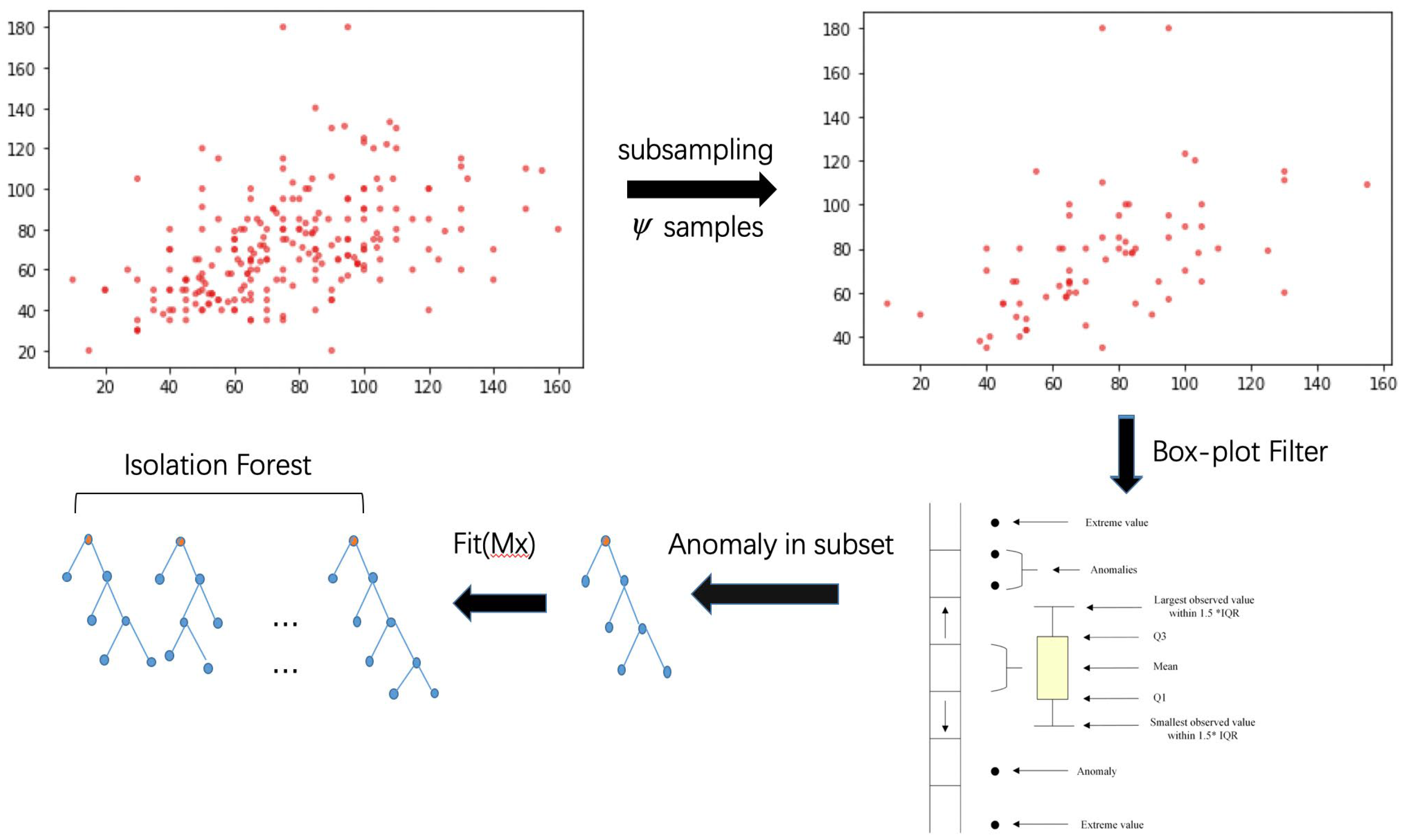
The BS-iForest algorithm first uses the box plot method to predict whether there are anomaly data points in the subsample set that are selected randomly to be the roots of trees. If there is an anomaly data point according to the results of the box plot for the subsample set, a tree rooted at the node will be created; otherwise, the iTree would not be created to reduce randomness. Secondly, since each tree has the same voting weight, BS-iForest selects trees that have higher accuracies to compose isolation forests to improve detection capability. Lastly, in the situation that path length intervals of positive samples intersect with path length intervals of negative samples, BS-iForest makes a judgment based on a combination of the first n samples that have the highest similarities.

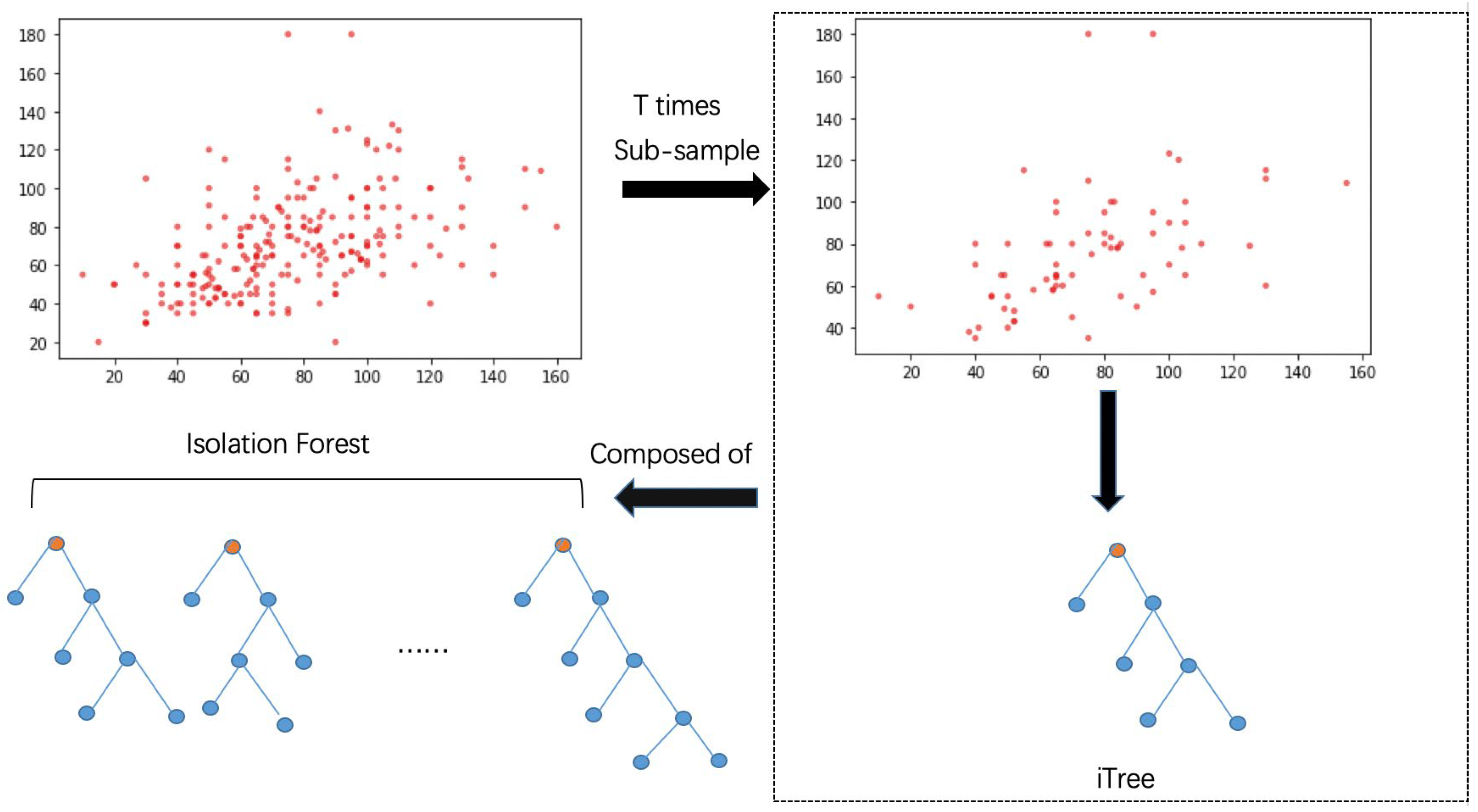
BS-iForest is based on an Isolation Forest algorithm adding phases to promote the detection ability. The intuitive differences between the standard Isolation Forest algorithm and BS-iForest are displayed in Figure 1 and Figure 2.

The number of trees, t, and sub-sampling size, ψ, are two parameters that should be manually set. Firstly, subsampling by not putting back for T times. Then, an isolation tree is constructed based on each sub-sample set, and the isolation trees selected according to fitness form an isolation forest. Finally, the anomaly score of each instance is used in the evaluation stage to identify anomalies.

As mentioned above, the traditional Isolation Forest algorithm has shortcomings such as strong randomness, poor stability, and weak performance when data lies in the intersection between positive sample path length interval and negative sample path length interval. Therefore, this paper proposes a box-plot-based Isolation Forest algorithm, known as BS-iForest. Figure 2 shows the process diagram of BS-iForest.

The pseudo-code of BS-iForest is shown in the following Algorithm 1:

Algorithm 1: BS-iForest(X,t,$\psi$)

Inputs: X—input data, t—number of trees, $\psi$—sub-sampling size Output: a set of BS-iForest trees 1: intialize Forest 2: set height limit l = ceiling(${\log }_2\psi$) 3: i = 1 4: while i <= t { 5: X’$\leftarrow$sample(X,$\psi$){ 6: if(box-plot-filter(X’)) 7: Forest$⟵$Forest $\cup$ iTree(X’,0,l) 8: i = i + 1 } 9: else continue 10:} 11: for j = 1 to iTrees_num in Forest 12: compute(fit(iTree[j]) 13: end for 14: select top k iTrees for BS_iForest //k < t 15: return BS-iForest

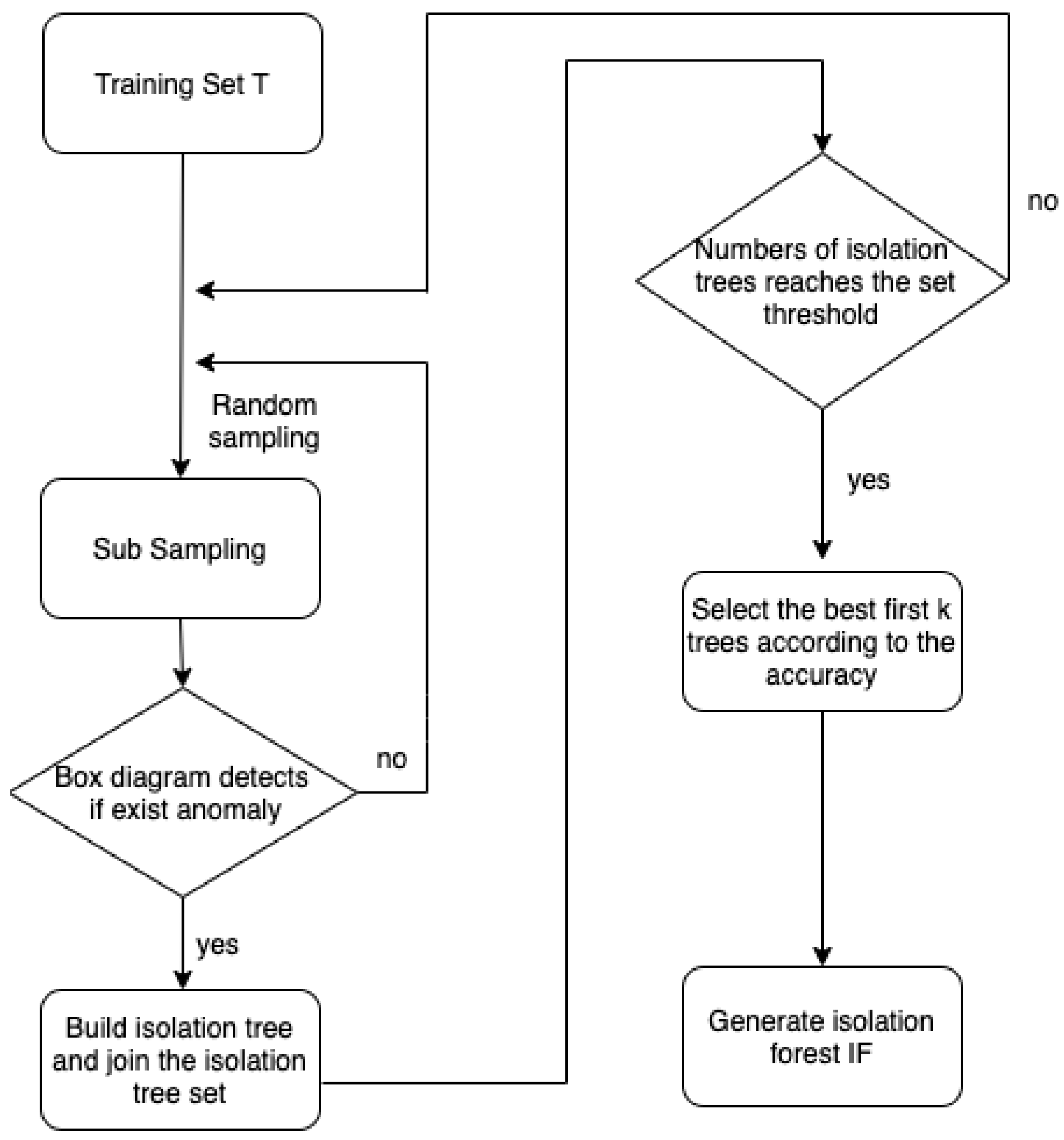
As described in the pseudo-code above, the main idea of the BS-iForest algorithm is to use the statistical method to judge whether the currently randomly sub-sampled set is more likely to have outliers. If so, the subsample set is used to build an isolation tree; otherwise, the isolation tree would not be constructed. Then, the algorithm continues to resample, which reduces the randomness. Because the voting weight of each isolation tree is the same, BS-iForest selects an isolation tree with the highest accuracy in the training set to form the forest and effectively improves the anomaly detection ability of the isolation forest. Finally, for the intersection of positive and negative sample path lengths, BS-iForest uses the current sample path to jointly determine the maximum value of the positive sample path, the minimum value of the negative sample path, and the previous sample distance, which improves the accuracy of the isolation forest.

The construction method of the isolation tree is to randomly select y samples from a given set with samples as the root node of the isolation tree and then randomly select a feature and separation value. Therefore, for such one-dimensional data, the abnormality of the data distribution can be detected through the box plot, and it can be judged whether the data on the feature is abnormal.

First, the box plot graph is generated on the subsample set of the root node. If the outcome contains values distributed outside the upper and lower limits, it indicates that the subsample set contains exceptions, and an isolation tree will be built. If the outcome contains no outliers, then no isolation tree is created.

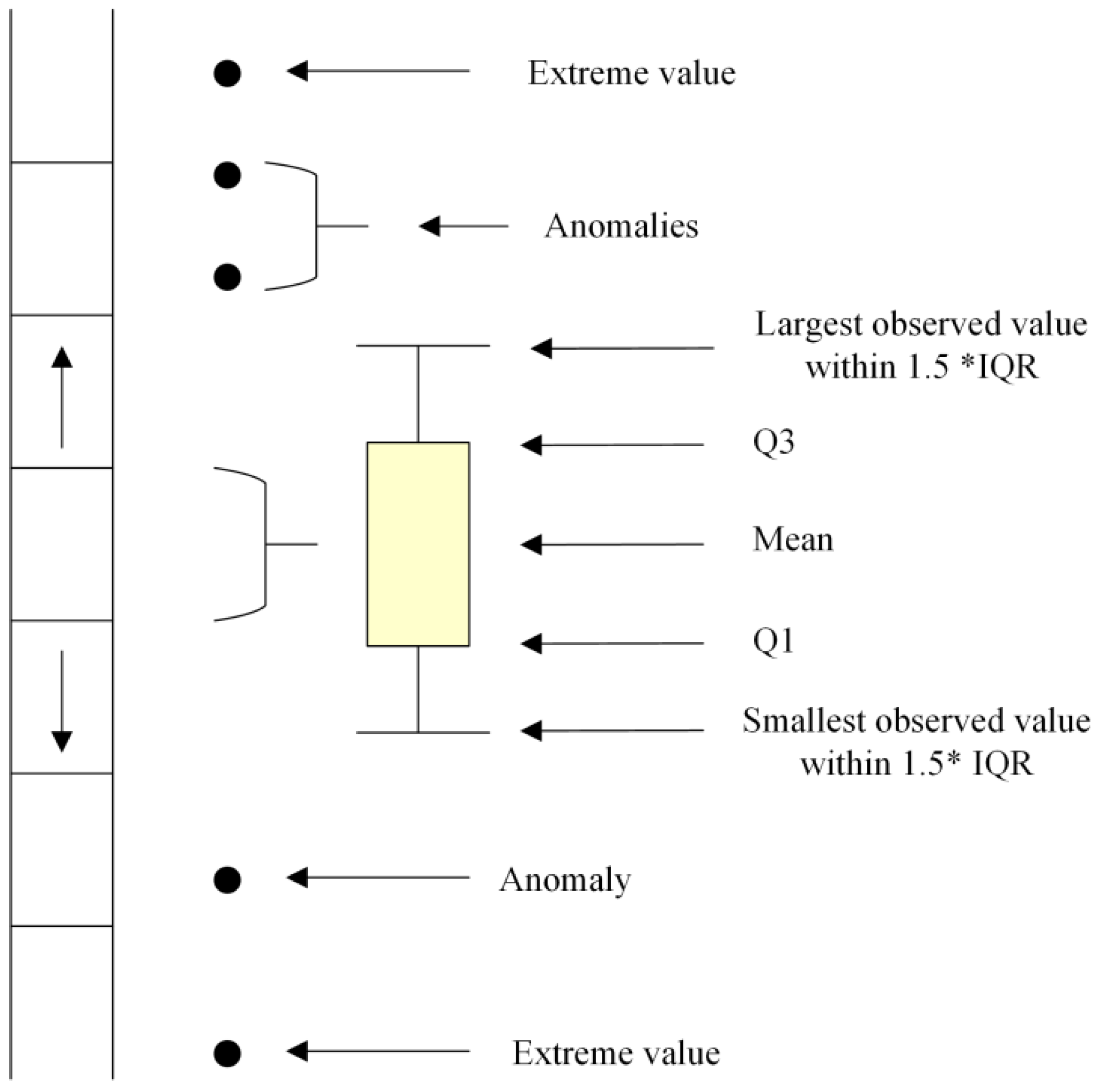
Box diagrams, also known as box whisker diagrams, are a general method for detecting abnormal values. The structure is shown in Figure 3. The median of the sample data is at the center of the box plot, the length of the box represents the interquartile range, the lower edge is the lower quartile ($Q3$), the lower edge is the lower quartile ($Q1$), and both ends of the box are outlier cutoff points, which is called the inner limit. The outliers defined in the box chart are data points distributed outside the upper and lower limits. Being different from the traditional 3-sigma method and the Z-fraction method, the box graph method can not only be used as the sample set subject to a normal distribution but also has a good effect on the sample set not subject to a normal distribution and has strong universality.

The fitness of each isolated tree is then calculated. The training set is divided into n disjoint subsets, n − 1 subsets are used for training each isolation tree, and the remaining subset is used for testing. Finally, the average accuracy of all subsets is calculated as the final accuracy of the isolation tree. The correlation between each isolation tree and all trees except itself is computed. In the case of a single sample, the correlation calculation formula between trees is as Equation (1):

$$s_e\left(M_x,M_y\right)=1-{\delta }_e\left(M_x,M_y\right)$$

(1)

where $e$ represents the sample, and $M_x$ and $M_y$ are two different isolation trees. See the calculation formula of ${\delta }_e\left(M_x,M_y\right)$ in Formula (2):

$${\delta }_e\left(M_x,M_y\right)=\frac{1}{\left|C\right|}{\displaystyle \sum }_{j=1}^{\left|C\right|}\frac{P{D}_{xj}\left(e\right)-P{D}_{yj}\left(e\right)}{R_j\left(e\right)}$$

(2)

where $\left|C\right|$ represents the number of categories, $P{D}_{xj}\left(e\right)$ represents the posterior probability of classifier $x$ on sample $e$ on class $j$, $P{D}_{yj}\left(e\right)$ represents the posterior probability of classifier $y$ on sample $e$ on class $j$, and $R_j\left(e\right)$ represents the extreme difference in the posterior probability of sample $e$ on class $j$. This is calculated using Formula (3):

$$R_j\left(e\right)=max\left\{P{D}_{1j}\left(e\right),\dots \dots ,P{D}_{Nj}\left(e\right)\right\}-min\left\{P{D}_{1j}\left(e\right),\dots \dots ,P{D}_{Nj}\left(e\right)\right\}$$

(3)

Based on the single-sample correlation, it is easy to obtain the correlation between the classifiers, that is, the arithmetic mean of the sample similarity in the entire set. This is calculated using Formula (4):

$$s_E\left(M_x,M_y\right)=\frac{1}{\left|E\right|}{\displaystyle \sum }_{e\in E}{s}_e\left(M_x,M_y\right)$$

(4)

where $\left|E\right|$ is the number of samples in the verification set.

After calculation of the correlations for every two isolation trees in the forest, the arithmetic average of each isolation tree and all the correlations except itself is considered as the final similarity of the isolation tree itself. The fitness of each isolation tree is calculated by similarity and accuracy. The calculation formula as Equation (5):

$$fit\left(M_x\right)=\frac{1}{sim\left(M_x\right)}\times (\frac{1}{1-acc{\left(M_x\right)}^2}-1)$$

(5)

According to the fitness, the best $K$ isolation trees are selected to form an isolation forest. The training process of BS-iForest is shown in Figure 4:

Finally, the path length interval of positive samples is calculated according to the original training set in [pMin, pMax], and the path length interval of negative samples is [nMin, nMax]. If there is no intersection between the path length intervals of positive and negative samples, that is, pMin > nMax, the median between [pMax, nMin] is taken as the judgment threshold φ. If the path length is bigger than φ, the sample is considered abnormal. If the path length interval of positive and negative samples has an intersection, that is, pMin <= nMax, the sample is judged as normal. Then, the Euclidean distance is computed from the previous sample to the current one. The mode of the classification result of this sample is used as the classification result of the current sample.

4. Discussion

4.1. Dataset

The datasets used in this paper are the actual campus sensor data (Campus-CRS) and the dataset of Breast Cancer Wisconsin from the UCL dataset. The actual campus sensor dataset records data was collected by environmental sensors in data centers from November 2020 to April 2021. It has six dimensions with 27,066 records, including attributes such as temperature, humidity, and electric current. The BreastW dataset has 10 dimensions with 699 records, including information such as mass thickness, cell size uniformity, and cell shape uniformity. The details of the dataset are shown in

Table 6. Actual campus sensor dataset details.

Attributes	Description
voltage	Current server cabinet input voltage
current	Current server cabinet input current
power	Current server cabinet power
energy	Current server cabinet electric energy
temperature	Current server cabinet temperature
humidity	Current server cabinet humidity

and

Table 7. BreastW dataset details.

Attributes	Description
Sample-cn number	Sample code number (1–10)
Clump	Clump thickness (1–10)
Cell size	Uniformity of cell size (1–10)
Cell shape	Uniformity of cell shape (1–10)
MA	Marginal adhesion (1–10)
SECS	Single epithelial cell size (1–10)
Bare nuclei	Bare nuclei (1–10)
Bland-ch	Bland chromatin (1–10)
Normal-nuc	Normal nucleoli (1–10)
Mitoses	Mitoses (1–10)

:

As the dataset BreastW used in the experiment indeed is not a representative of the IoT system, it is used as a comparative dataset to determine whether this method can improve performance compared with the traditional Isolation Forest algorithm.

4.2. Experimental Parameter Setting

The experimental platform used in this paper is a Windows host with a 3.40 GHz CPU and 24.00 GB memory. The experimental program is written in Java. BS-iForest has two input parameters: the subsample size, $\psi$, and the number of items, $T$. The subsample size controls the size of the training data because when $\psi$ increases infinitely, it will increase the processing time and require more memory. This paper uses $\psi =256$ and $T=100$ as the experimental values.

4.3. Performance Metrics

In this paper, accuracy (ACC) and AUC (area under curve) are used as the evaluation metrics of algorithm performance. ACC describes the proportion of all correctly classified samples in all samples, and AUC is the receiver operating characteristic curve (ROC) of the area enclosed by the coordinate axis. The abscissa of the ROC curve is the proportion of negative cases judged as positive, that is, the false-positive rate; the ordinate is the proportion of positive samples judged as positive, that is, the true positive rate. The larger the ACC value, the higher the accuracy of the model, and the stronger the generalization ability of the learning model. When calculating the AUC, the forest composed of the first 30 isolation trees was used to calculate the BS-iForest AUC of the method.

4.4. Analysis of Experimental Results

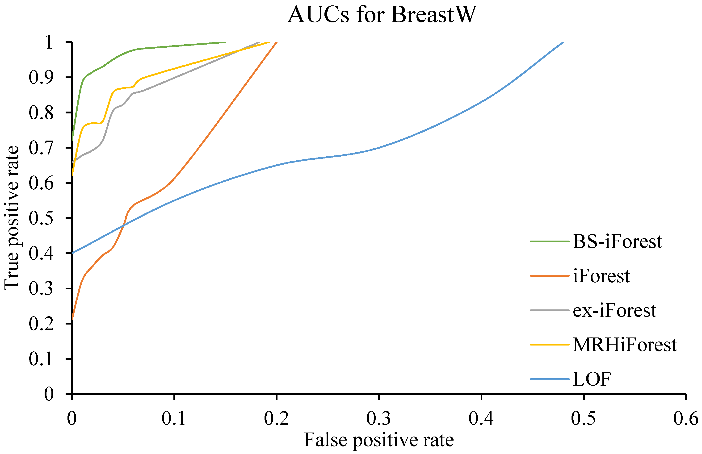
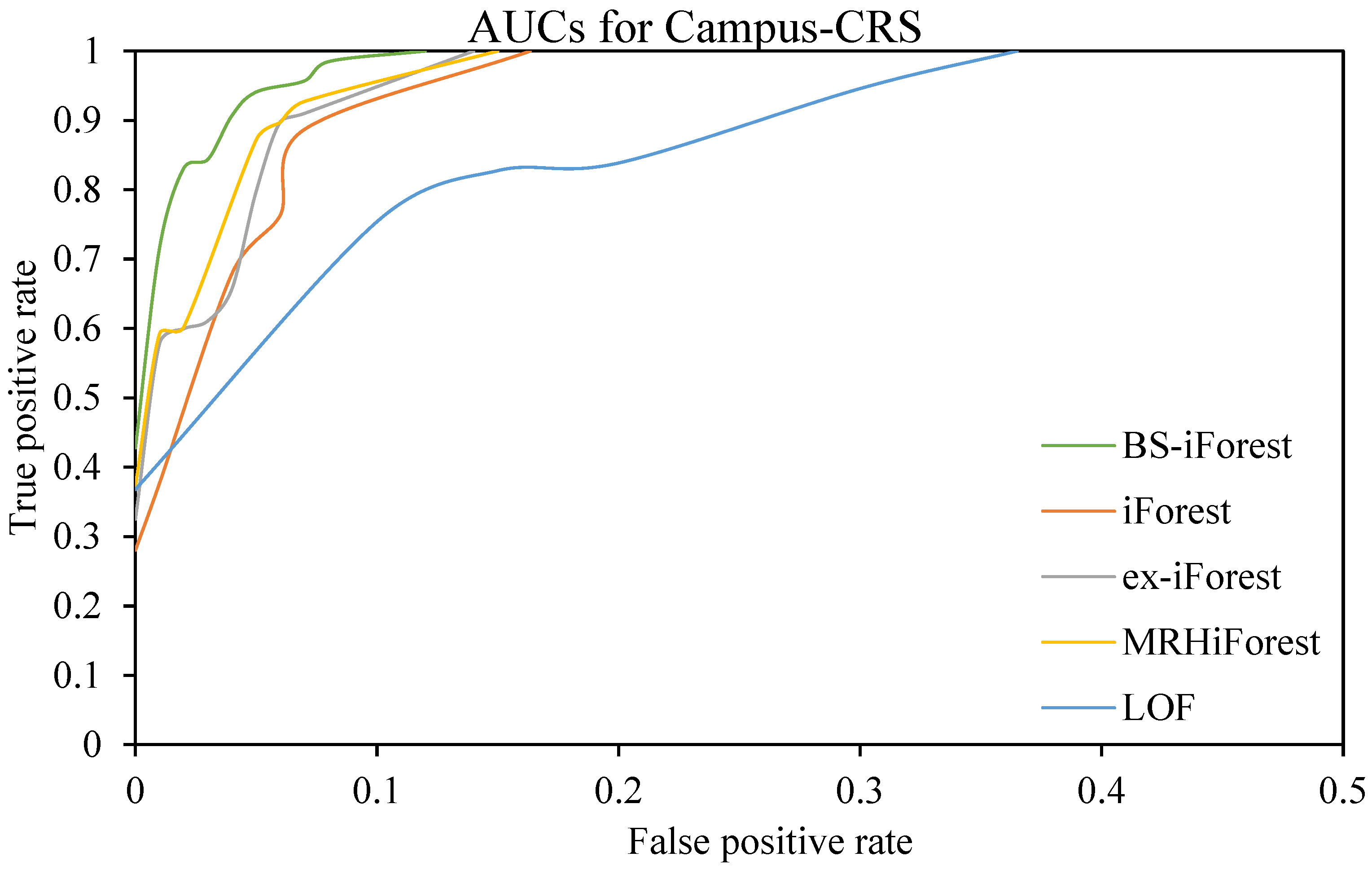
In this section, the improved anomaly detection method BS-iForest based on isolation forest is compared with the traditional iForest, ex-iForest [39], MRH-iForest, and local outlier factor (LOF) algorithms on the Campus-CRS dataset and BreastW public dataset. Figure 5 and Figure 6 shows the ROC curves of the Campus-CRS and BreastW datasets.

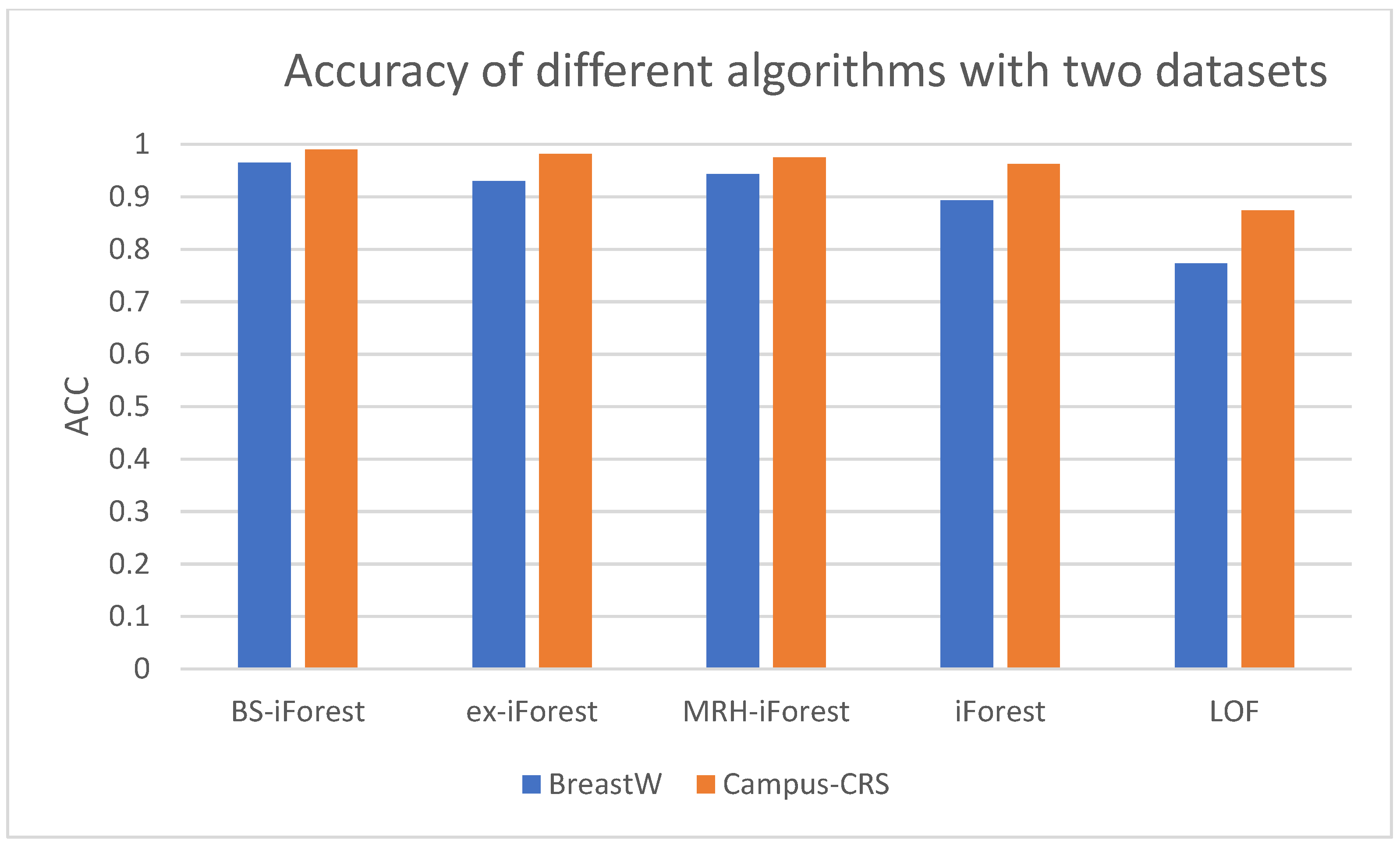
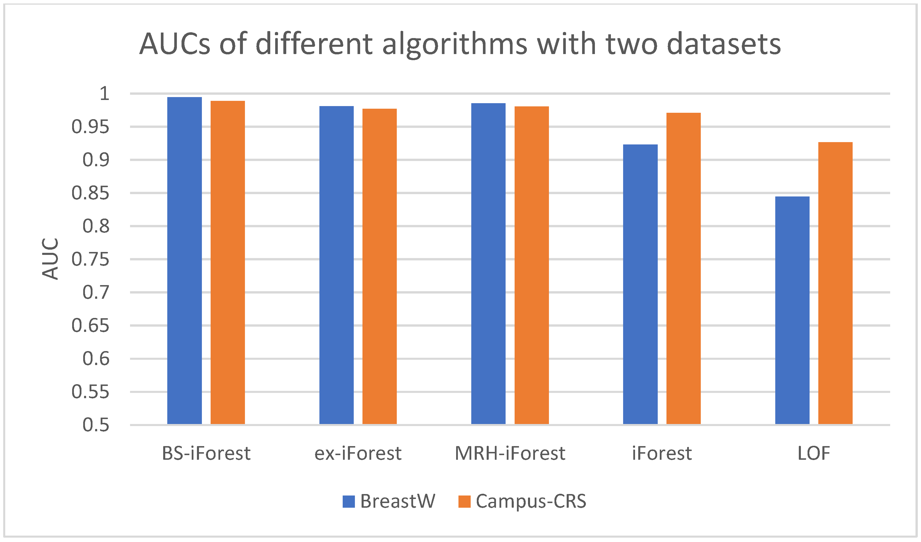
To make the results more objective, each algorithm was executed 10 times on different datasets, and then the arithmetic average was taken as the final result. The corresponding accuracy and AUC values are detected on different datasets, and the results are listed in Figure 7 and Figure 8. Among the five algorithms, BS-iForest has the largest AUC value on the two datasets, which also means that on the two datasets, BS-iForest shows the best performance on sensitivity.

The experiments on the datasets BreastW and Campus-CRS indicate that BS-iForest produces the best performance on accuracy and the AUC metric. Indeed, the difference in AUC between BS-iForest and MRH-iForest is very small.

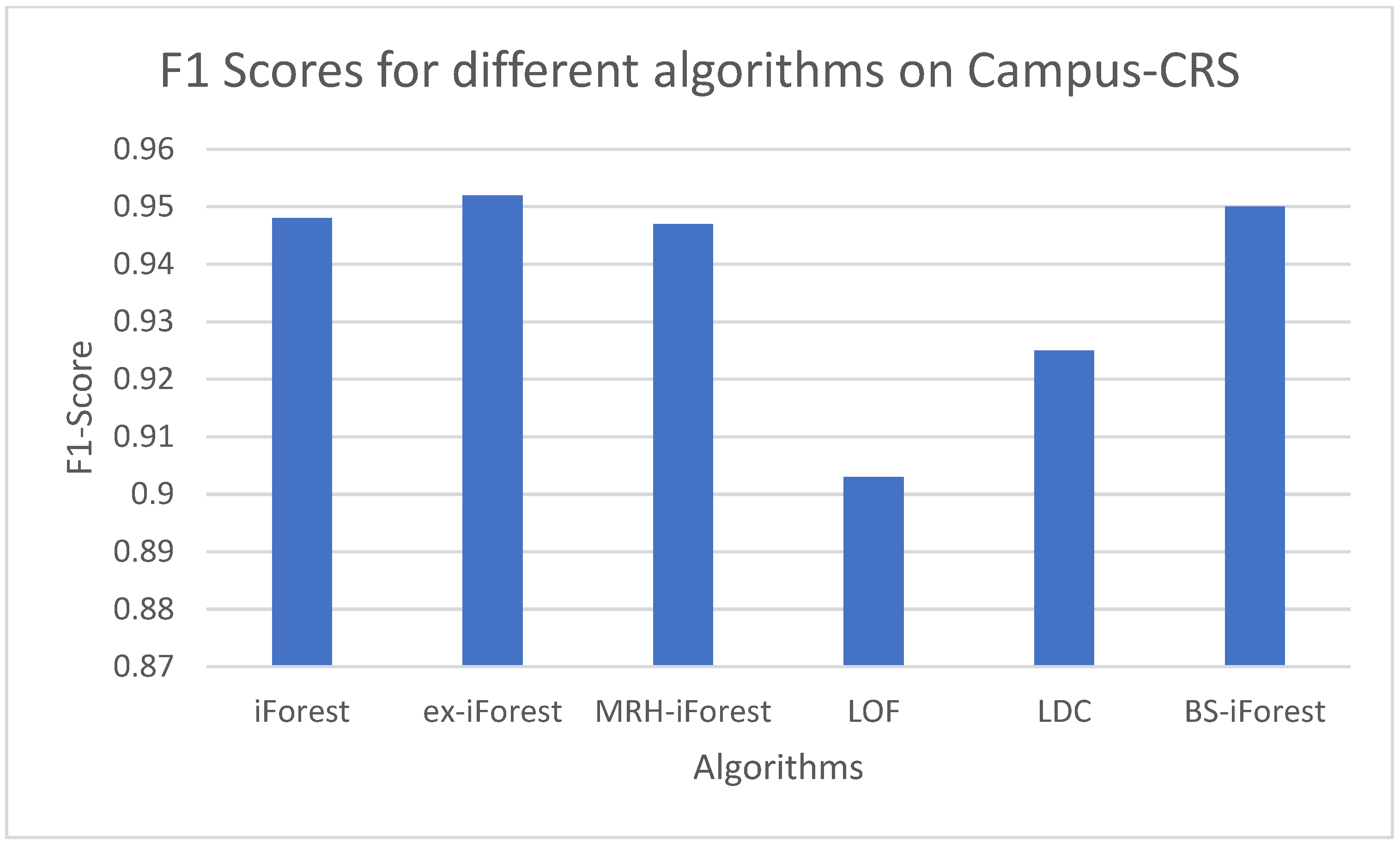
For the five algorithms, this paper conducts an F1 score evaluation. As shown in Figure 9, the experimental results show that in the Campus-CRS data set, the F1 score of BS-iForest is 0.95, which is slightly lower than that of ex-iForest.

From the experimental results, we see that the overall performance of BS-iForest is better than that of the other four algorithms, and its anomaly detection effect is better. The AUCs on the BreastW dataset and campus CRS dataset reached 0.9947 and 0.989, respectively, which increased by 7.7% and 1.5% compared with the traditional forest method. The accuracy rates were 0.9653 and 0.9896, respectively, which improved by 7.18% and 2.76% compared with the traditional iForest method. This is mainly because BS-iForest preliminarily screens sub-sampling sets through box plots, and uses sub-sampling sets that are more likely to have outliers for training. At the same time, isolated trees with high accuracy on the training set are selected to form a forest. The samples in the intersection of positive and negative path length intervals are jointly judged by adjacent data points, which improves the abnormal detection ability of the algorithm.

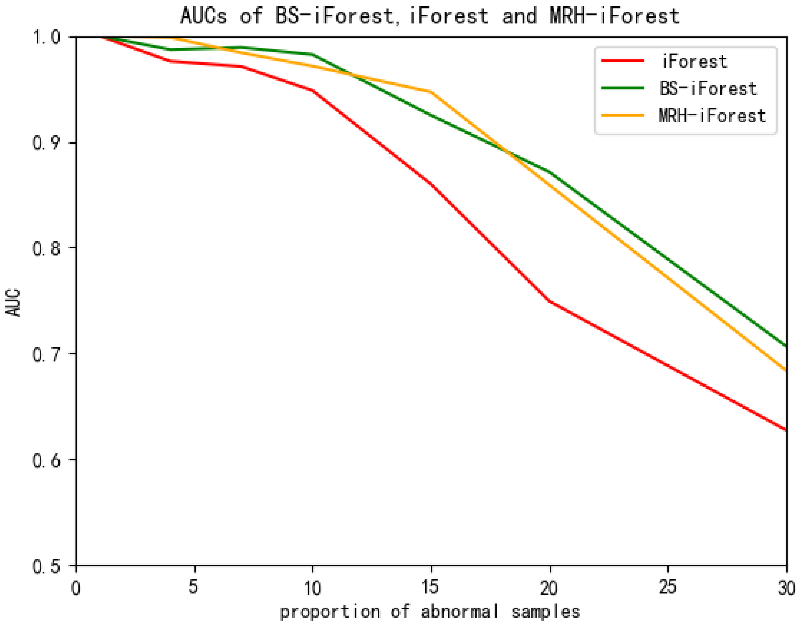
In order to test the stability of the algorithm on abnormal data, abnormal points were gradually added to the Campus-CRS data set, and the AUC curves of BS-iForest, MRH-iForest, and iForest algorithms were calculated. The experimental results are shown in Figure 10. The results show that when the proportion of outliers is low, BS-iForest and MRH-iForest have little difference in AUC indicators. When the proportion of abnormal data increases, BS-IForest is slightly higher than MRH-iForest in AUC indicators. However, when BS-iForest is compared with the standard iForest algorithm, iForest has a higher AUC index regardless of the proportion of outliers.

The AUC curves of the three algorithms show that the overall performance of BS-iForest is better than that of traditional iForest, indicating that the algorithm can better isolate abnormal data points, while BS-iForest outperforms MRH-iForest with a high proportion of abnormal samples. When the proportion of abnormal data points is 15%, the AUC of iForest decreases below 0.9; and when the proportion of abnormal data points is 20%, the AUC of BS-iForest drops below 0.9, and the AUC of iForest is 0.74. The stability of BS-iForest is better than that of iForest, and the continuous decline in AUC is related to the gradual increase in the proportion of abnormal points, while the applicable premise of traditional iForest is that the distribution of deviant data points in the dataset is sparse.

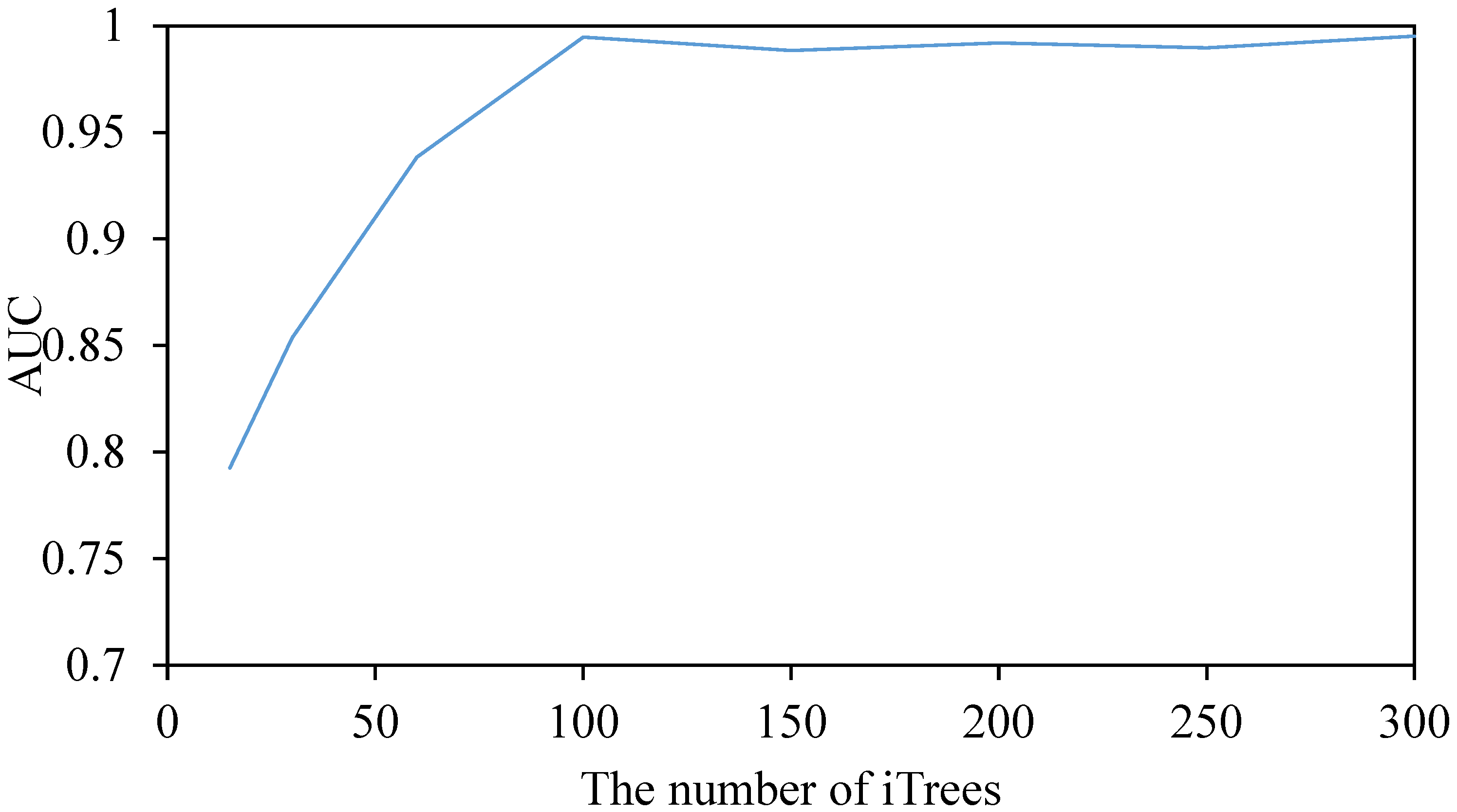
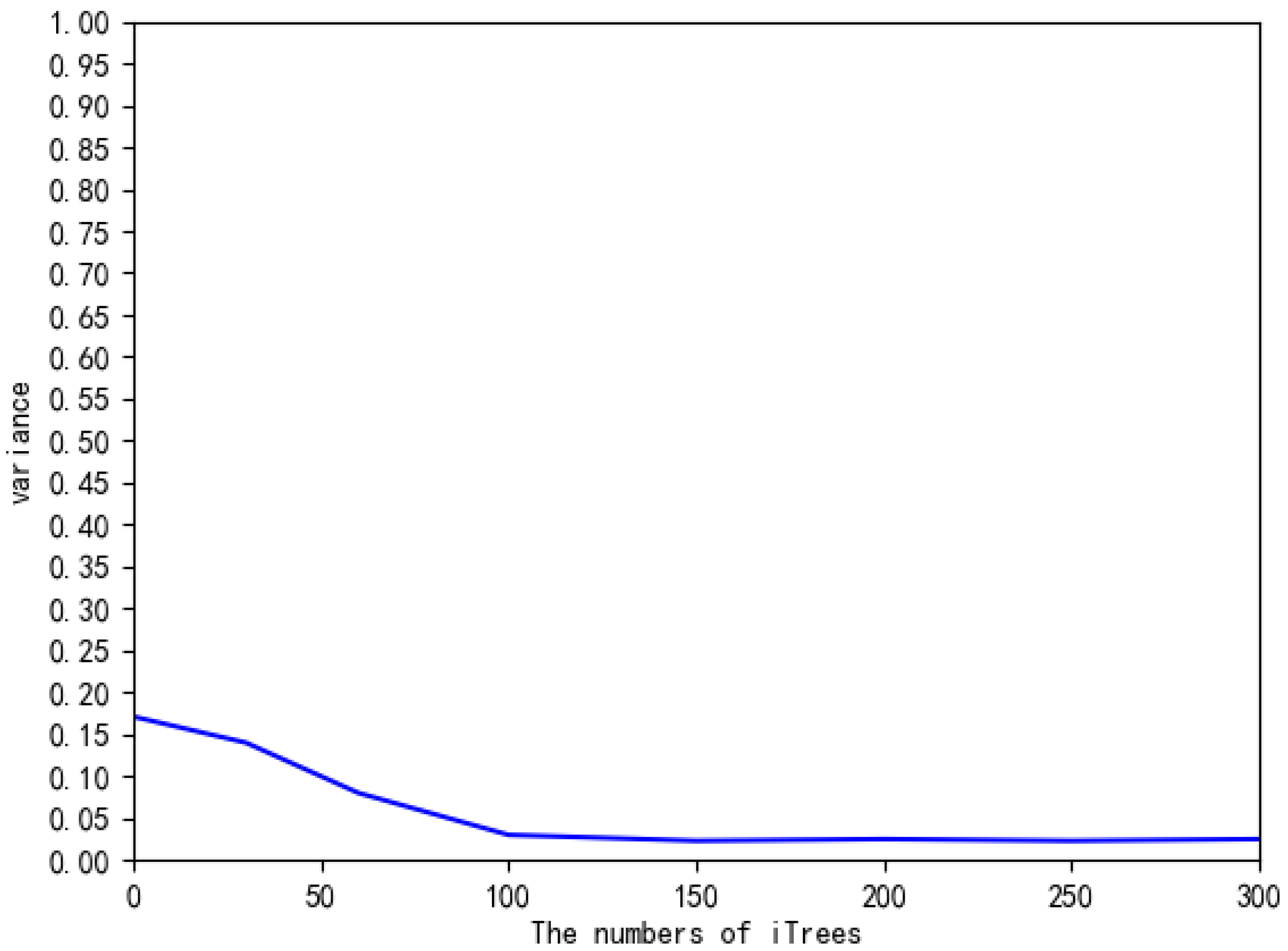
In the experiments above, BS-iForest set the number of iTrees to 100. For further discussion on the optimal values of iTree in BS-iForest, let T be 15, 30, 60, 100, 150, 200, 250, and 300 in the BreastW dataset, calculate the AUC of BS-iForest one by one, take the arithmetic average of the five experimental results as the final result, and take the variance as the stability index. The experimental results are shown in Figure 11 and Figure 12.

Randomness is the main reason for the unstable performance of iForest. Figure 11 and Figure 12 show that when the number of different iTrees is small, the performance and stability of BS-iForest are enhanced with the growth of the number of iTrees. When $T=100$, the growth of AUC is gradually flat and the variance is gradually reduced. Then, the performance of the algorithm is no longer sensitive to the increase in the number of iTrees. This is mainly because BS-iForest is an integrated learning method. Some iTrees with weak performance will affect the final detection results, and the stability will increase with the increase in iTrees. In addition, the number of iTrees is too small to build more iTrees generated by sampling sets with abnormal samples, which cannot play a part in the advantage of preliminary screening by box diagrams.

5. Conclusions

Aiming at the problems of strong randomness, poor stability, and low anomaly detection accuracy of traditional iForest, a data anomaly detection method, BS-iForest, is proposed in this paper. Compared with the traditional iForest algorithm, this method first judges the data distribution of the subsampling set according to the box plot graph, then uses the subsampling set with more likely abnormal samples to train the isolation tree, reduces the influence of irrelevant samples on the isolation outliers, and improves the accuracy of anomaly detection. For the construction of the spanning isolation tree, some data points with poor performance are screened out according to the accuracy in the training set, which improves the stability. For the samples that intersect the path length interval of the positive and negative examples, the data points with the highest similarity are used for joint judgment, which improves the anomaly detection performance of the algorithm. Many experiments were carried out on the BreastW dataset and Campus-CRS dataset. The results show that the improved Isolation Forest algorithm recommended in this paper has significantly improved the accuracy and enhanced the stability. In future work, the local anomaly detection ability of the isolation forest can be improved because the isolation forest is not sensitive to local outliers.

References

- Ayadi, A.; Ghorbel, O.; Obeid, A.M.; Abid, M. Outlier detection approaches for wireless sensor networks: A survey. Comput. Netw. 2017, 129, 319–333. [Google Scholar] [CrossRef]
- Garcia-Font, V.; Garrigues, C.; Rifà-Pous, H. Difficulties and Challenges of Anomaly Detection in Smart Cities: A Laboratory Analysis. Sensors 2018, 18, 3198. [Google Scholar] [CrossRef] [Green Version]
- Liu, F.T.; Ting, K.M.; Zhou, Z.-H. Isolation-based anomaly detection. ACM Trans. Knowl. Discov. Data (TKDD) 2012, 6, 1–39. [Google Scholar] [CrossRef]
- Hariri, S.; Kind, M.C.; Brunner, R.J. Extended Isolation Forest. IEEE Trans. Knowl. Data Eng. 2021, 33, 1479–1489. [Google Scholar] [CrossRef] [Green Version]
- Zivkovic, Z. Improved adaptive Gaussian mixture model for background subtraction. In Proceedings of the 17th International Conference on Pattern Recognition (ICPR), Cambridge, UK, 23–26 August 2004; Volume 22, pp. 28–31. [Google Scholar]
- Karczmarek, P.; Kiersztyn, A.; Pedrycz, W.; Al, E. K-Means-based isolation forest. Knowl.-Based Syst. 2020, 195, 105659. [Google Scholar] [CrossRef]
- Laksono, M.A.T.; Purwanto, Y.; Novianty, A. DDoS detection using CURE clustering algorithm with outlier removal clustering for handling outliers. In Proceedings of the 2015 International Conference on Control, Electronics, Renewable Energy and Communications (ICCEREC), Bandung, Indonesia, 27–29 August 2015; pp. 12–18. [Google Scholar]
- Guha, S.; Rastogi, R.; Shim, K. Rock: A robust clustering algorithm for categorical attributes. Inf. Syst. 2000, 25, 345–366. [Google Scholar] [CrossRef]
- Saeedi Emadi, H.; Mazinani, S.M. A Novel Anomaly Detection Algorithm Using DBSCAN and SVM in Wireless Sensor Networks. Wirel. Pers. Commun. 2018, 98, 2025–2035. [Google Scholar] [CrossRef]
- Prodanoff, Z.G.; Penkunas, A.; Kreidl, P. Anomaly Detection in RFID Networks Using Bayesian Blocks and DBSCAN. In Proceedings of the 2020 SoutheastCon, Raleigh, NC, USA, 28–29 March 2020; pp. 1–7. [Google Scholar]
- Yin, C.; Zhang, S. Parallel implementing improved k-means applied for image retrieval and anomaly detection. Multimed. Tools Appl. 2017, 76, 16911–16927. [Google Scholar] [CrossRef]
- Wang, Z.; Zhou, Y.; Li, G. Anomaly Detection by Using Streaming K-Means and Batch K-Means. In Proceedings of the 2020 5th IEEE International Conference on Big Data Analytics (ICBDA), Xiamen, China, 8–11 May 2020; pp. 11–17. [Google Scholar]
- Ying, S.; Wang, B.; Wang, L.; Li, Q.; Zhao, Y.; Shang, J.; Huang, H.; Cheng, G.; Yang, Z.; Geng, J. An Improved KNN-Based Efficient Log Anomaly Detection Method with Automatically Labeled Samples. ACM Trans. Knowl. Discov. Data 2021, 15, 34. [Google Scholar] [CrossRef]
- Wang, B.; Ying, S.; Cheng, G.; Wang, R.; Yang, Z.; Dong, B. Log-based anomaly detection with the improved K-nearest neighbor. Int. J. Softw. Eng. Knowl. Eng. 2020, 30, 239–262. [Google Scholar] [CrossRef]
- Xu, S.; Liu, H.; Duan, L.; Wu, W. An Improved LOF Outlier Detection Algorithm. In Proceedings of the 2021 IEEE International Conference on Artificial Intelligence and Computer Applications (ICAICA), Dalian, China, 28–30 June 2021; pp. 113–117. [Google Scholar]
- Kriegel, H.-P.; Kröger, P.; Schubert, E.; Zimek, A. LoOP: Local outlier probabilities. In Proceedings of the 18th ACM conference on Information and Knowledge Management, Hong Kong, China, 2–6 November 2009; pp. 1649–1652. [Google Scholar]
- Tan, R.; Ottewill, J.R.; Thornhill, N.F. Monitoring statistics and tuning of kernel principal component analysis with radial basis function kernels. IEEE Access 2020, 8, 198328–198342. [Google Scholar] [CrossRef]
- Yokkampon, U.; Chumkamon, S.; Mowshowitz, A.; Hayashi, E. Anomaly Detection in Time Series Data Using Support Vector Machines. In Proceedings of the International Conference on Artificial Life & Robotics (ICAROB2021), Online, 21–24 January 2021; pp. 581–587. [Google Scholar]
- Choi, Y.-S. Least squares one-class support vector machine. Pattern Recognit. Lett. 2009, 30, 1236–1240. [Google Scholar] [CrossRef]
- Yu, Q.; Jibin, L.; Jiang, L. An improved ARIMA-based traffic anomaly detection algorithm for wireless sensor networks. Int. J. Distrib. Sens. Netw. 2016, 12, 9653230. [Google Scholar] [CrossRef] [Green Version]
- Ghorbel, O.; Ayedi, W.; Snoussi, H.; Abid, M. Fast and Efficient Outlier Detection Method in Wireless Sensor Networks. IEEE Sens. J. 2015, 15, 3403–3411. [Google Scholar] [CrossRef]
- Li, Q.; Li, R.; Ji, K.; Dai, W. Kalman filter and its application. In Proceedings of the 2015 8th International Conference on Intelligent Networks and Intelligent Systems (ICINIS), Tianjin, China, 1–3 November 2015; pp. 74–77. [Google Scholar]
- Li, H.; Achim, A.; Bull, D. Unsupervised video anomaly detection using feature clustering. IET Signal Process. 2012, 6, 521–533. [Google Scholar] [CrossRef]
- Amidi, A. Arima based value estimation in wireless sensor networks. Int. Arch. Photogramm. Remote Sens. Spat. Inf. Sci. 2014, 40, 41. [Google Scholar] [CrossRef] [Green Version]
- Schmidt, F.; Suri-Payer, F.; Gulenko, A.; Wallschläger, M.; Acker, A.; Kao, O. Unsupervised anomaly event detection for cloud monitoring using online arima. In Proceedings of the 2018 IEEE/ACM International Conference on Utility and Cloud Computing Companion (UCC Companion), Zurich, Switzerland, 17–20 December 2018; pp. 71–76. [Google Scholar]
- Ren, H.; Ye, Z.; Li, Z. Anomaly detection based on a dynamic Markov model. Inf. Sci. 2017, 411, 52–65. [Google Scholar] [CrossRef]
- Honghao, W.; Yunfeng, J.; Lei, W. Spectrum anomalies autonomous detection in cognitive radio using hidden markov models. In Proceedings of the 2015 IEEE Advanced Information Technology, Electronic and Automation Control Conference (IAEAC), Chongqing, China, 19–20 December 2015; pp. 388–392. [Google Scholar]
- Yuanyang, P.; Guanghui, L.; Yongjun, X.; software. Abnormal data detection method for environmental sensor networks based on DBSCAN. Comput. Appl. Softw. 2012, 29, 69–72+111. [Google Scholar]
- Wazid, M.; Das, A.K. An efficient hybrid anomaly detection scheme using K-means clustering for wireless sensor networks. Wirel. Pers. Commun. 2016, 90, 1971–2000. [Google Scholar] [CrossRef]
- Duan, D.; Li, Y.; Li, R.; Lu, Z. Incremental K-clique clustering in dynamic social networks. Artif. Intell. Rev. 2012, 38, 129–147. [Google Scholar] [CrossRef]
- Zhang, K.; Hutter, M.; Jin, H. A new local distance-based outlier detection approach for scattered real-world data. In Proceedings of the Pacific-Asia Conference on Knowledge Discovery and Data Mining, Bangkok, Thailand, 27–30 April 2009; pp. 813–822. [Google Scholar]
- Breunig, M.M.; Kriegel, H.-P.; Ng, R.T.; Sander, J. LOF: Identifying density-based local outliers. In Proceedings of the 2000 ACM SIGMOD International Conference on Management of Data, Dallas, TX, USA, 15–18 May 2000; pp. 93–104. [Google Scholar]
- Abid, A.; Kachouri, A.; Mahfoudhi, A. Anomaly detection through outlier and neighborhood data in Wireless Sensor Networks. In Proceedings of the 2016 2nd International Conference on Advanced Technologies for Signal and Image Processing (ATSIP), Monastir, Tunisia, 21–23 March 2016; pp. 26–30. [Google Scholar]
- Bosman, H.H.W.J.; Iacca, G.; Tejada, A.; Wörtche, H.J.; Liotta, A. Spatial anomaly detection in sensor networks using neighborhood information. Inf. Fusion 2017, 33, 41–56. [Google Scholar] [CrossRef]
- Xie, M.; Hu, J.; Han, S.; Chen, H.H. Scalable Hypergrid k-NN-Based Online Anomaly Detection in Wireless Sensor Networks. IEEE Trans. Parallel Distrib. Syst. 2013, 24, 1661–1670. [Google Scholar] [CrossRef]
- Luo, Z.; Shafait, F.; Mian, A. Localized forgery detection in hyperspectral document images. In Proceedings of the 2015 13th International Conference on Document Analysis and Recognition (ICDAR), Nancy, France, 23–26 August 2015; pp. 496–500. [Google Scholar]
- Xu, D.; Wang, Y.; Meng, Y.; Zhang, Z. An improved data anomaly detection method based on isolation forest. In Proceedings of the 2017 10th International Symposium on Computational Intelligence and Design (ISCID), Hangzhou, China, 9–10 December 2017; pp. 287–291. [Google Scholar]
- Xuxiang, W.L.Q.H.B. Multidimensional Data Anomaly Detection Method Based on Fuzzy Isolated Forest Algorithm. Comput. Digit. Eng. 2020, 48, 862–866. [Google Scholar]
- Zhou, J.C. Satellite Anomaly Detection Based on Unsupervised Algorithm. Master’s Thesis, Wuhan University, Wuhan, China, May 2020. [Google Scholar]
Figure 1.
The process diagram of standard Isolation Forest algorithm.
Figure 2.
Process diagram of BS-iForest.
Figure 3.
Box diagram structure.
Figure 4.
Flow chart of BS iForest training phase.
Figure 5.
BreastW dataset test results.
Figure 6.
Campus-CRS dataset test results.
Figure 7.
Accuracy on different datasets.
Figure 8.
AUCs on different datasets.
Figure 9.
F1 Scores for different algorithms on Campus-CRS.
Figure 10.
AUCs of BS-iForest, MRHi-Forest, and iForest in different numbers of outlier samples.
Figure 11.
AUC of BS-iForest under different numbers of isolation trees.
Figure 12.
Variance of BS-iForest under different numbers of isolation trees.