A Computational Framework for 2D Crack Growth Based on the Adaptive Finite Element Method

Abstract

As a part of a damage tolerance assessment, the goal of this research is to estimate the two-dimensional crack propagation trajectory and its accompanying stress intensity factors (SIFs) using the adaptive finite element method. The adaptive finite element code was developed using the Visual Fortran language. The advancing-front method is used to construct an adaptive mesh structure, whereas the singularity is represented through construction of quarter-point single elements around the crack tip. To generate an optimal mesh, an adaptive mesh refinement procedure based on the posteriori norm stress error estimator is used. The splitting node strategy is used to model the fracture, and the trajectory follows the successive linear extensions for every crack increment. The stress intensity factors (SIFs) for each crack extension increment are calculated using the displacement extrapolation technique. The direction of crack propagation is determined using the theory of maximum circumferential stress. The present study is carried out for two geometries, namely a rectangular structure with two holes and one central crack, and a cracked plate with four holes. The results demonstrate that, depending on the position of the hole, the crack propagates in the direction of the hole due to the unequal stresses at the crack tip, which are caused by the hole’s influence. The results are consistent with other numerical investigations for predicting crack propagation trajectories and SIFs.

1. Introduction

For assessing the behavior of a broad range of engineering and physical concerns, the finite element method (FEM) has undoubtedly been the most popular and successful analytical approach. Studying crack propagation is one of FEM’s application areas. As a crack grows, components lose their ability to withstand external loads and eventually fail. A rigorous analysis of their durability and an estimation of operational life are required for the computational design of structural components and materials with embedded cracks. Numerous numerical techniques have proven successful in modeling and simulating engineering issues, such as fracture mechanics, where it can be difficult to find an optimal solution due to the singularity of the stress field near the crack tip. These include the extended finite element method (XFEM) [1,2,3,4], finite element method (FEM) [5,6,7,8], discrete element method (DEM) [9,10,11], mesh-free method [12], and boundary element method (BEM) [13]. Numerous software programs, including Ansys [14,15], ABAQUS [16], NASTRAN, FRANC3D, and COMSOL, which are well-known for being in three dimensions, have been developed with general-purpose finite elements, verified, and implemented for crack propagation simulation. These programs are now available to virtually everyone who requests and pays the required fees for them. Crack propagation may also be simulated using a variety of 2D simulation software, such as NASGRO, AFGROW, FRANC2D, and FASTRAN. In addition, a significant number of researchers have developed reliable methods for estimating the fatigue crack propagation in 2D linear elastic structures under mixed-mode loading [17,18,19,20]. Crack propagation is often simulated in LEFM by using the equivalent stress intensity factor. The stress intensity factors must be precisely evaluated to anticipate the behavior of crack growth. Numerous handbooks provide analytical SIF solutions for ideal crack configurations and loading conditions that could be used with simple and regular structures [21,22,23]. Nevertheless, in many structures, the configuration of fatigue cracks is often intricate and irregular, which results in a variety of distinct ways to fail. As a consequence, analytical solutions will not be able to accurately anticipate SIF solutions for these fatigue cracks, which can be estimated using the findings of the FEM. The displacement extrapolation technique [24,25] and the J-integral method [26,27,28] are the two approaches used most often to calculate SIFs. The trajectory of a crack’s propagation may be predicted using a variety of approaches including the theory of maximum circumferential stress, the theory of maximum energy release, and the theory of minimum strain-energy density. In this work, an automated adaptive mesh finite element is used to simulate mixed-mode crack propagation in the presence of holes using developed source code written in the Visual Fortran language. The outcomes acquired using the developed program are similar to those obtained using commercial fracture mechanics software, e.g., [29,30,31,32,33,34,35,36,37,38]. In regard to knowledge, utilizing source code is appropriate for at least two purposes: first, understanding the basic algorithm that it uses, and second, acquiring programming expertise in its development. This study also shows a scientific methodology that researchers may follow as a guideline to build their own programs at the lowest possible cost when compared to commercial software.

2. Procedure of the Developed Program

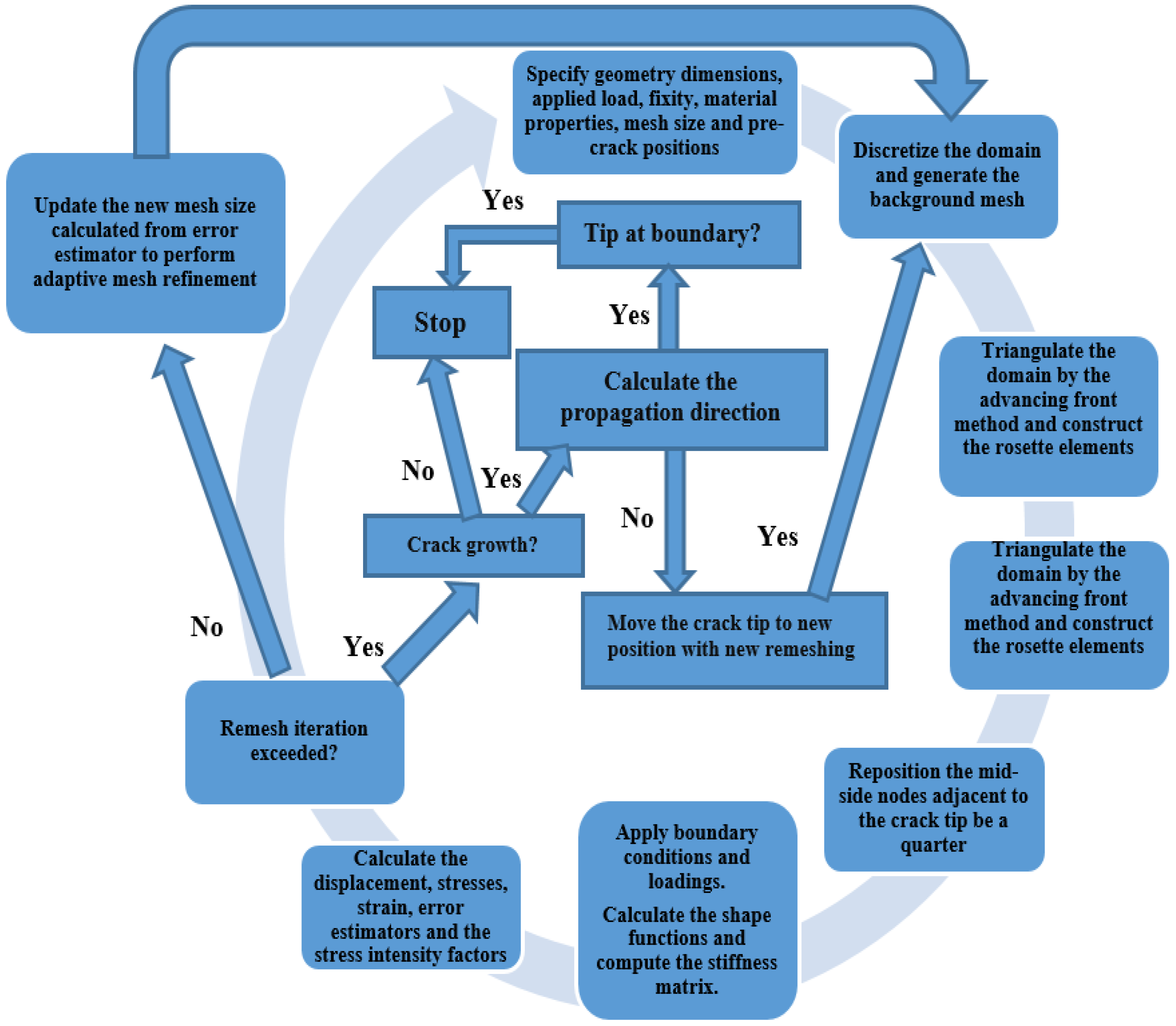
The geometrical dimensions, stresses, material characteristics, and other restrictions are first introduced into the 2D model of crack growth. Incremental stress analysis is performed using the FEM during the pre-processing stage. The SIFs are determined at each step of crack propagation using the displacement extrapolation technique (DET). The crack propagation trajectory is then estimated using the maximum circumferential stress theory (MCST). For the purpose of generating the mesh, the advancing-front method has been implemented. Using this procedure, it is necessary to define the domain boundaries, generate the elements, smooth the mesh, and renumber the nodes [39]. The error estimator provides an estimate of the particular scale of each element, and that estimate is utilized to control the mesh refinement process. The solution’s components, such as stresses, displacements, and strains, among others, are transferred from the old mesh onto the new mesh once the new mesh has been generated. Figure 1 depicts the computational strategy for the crack propagation program.

2.1. Crack-Kinking Criteria

In this study, the crack growth angle was calculated using the maximum circumferential stress theory [40]. According to this theory, when mixed-mode loading is applied to isotropic materials, the crack develops in a path that is normal to the direction of the maximum tangential tensile stress. According to this theory, the tangential stresses in polar coordinates are given by the following expressions [40,41]:

$$\begin{array}{l}{\sigma }_r = \frac{1}{\sqrt{2\pi r}}\cos (\theta /2)\left(K_I[1+{\sin }^2(\theta /2)]+\frac{3}{2}{K}_{II}\sin \theta -2K_{II}\tan (\theta /2)\right)\\ {\sigma }_{\theta }=\frac{1}{\sqrt{2\pi r}}\cos (\theta /2)\left[K_I{\cos }^2(\theta /2)-\frac{3}{2}{K}_{II}\sin \theta \right]\\ {\tau }_{r\theta }=\frac{1}{\sqrt{2\pi r}}\frac{\cos (\theta /2)}{2}\left[K_I\sin \theta +K_{II}(3\cos \theta -1)\right]\end{array}$$

(1)

where ${\sigma }_r$ represents the normal stress in the radial direction, ${\sigma }_{\theta }$ represents the normal stress in tangential direction, and ${\tau }_{r\theta }$ represents the shear stress.

By solving $d{\sigma }_{\theta }/d\theta =0$ for $\theta$, the result is expressed as:

$$K_I\sin \theta +K_{II}\left(3\cos \theta -1\right)=0$$

(2)

from which the kinking angle can be obtained as:

$$\theta ={\cos }^{-1} \left(\frac{3K_{II}^2+K_I\sqrt{K_I^2+8K_{II}^2}}{K_I^2+9K_{II}^2}\right)$$

(3)

To achieve the maximum stress associated with incremental crack expansion, the sign of $\theta$ must be opposed the sign of K_II [42].

2.2. Generation of the Background Mesh

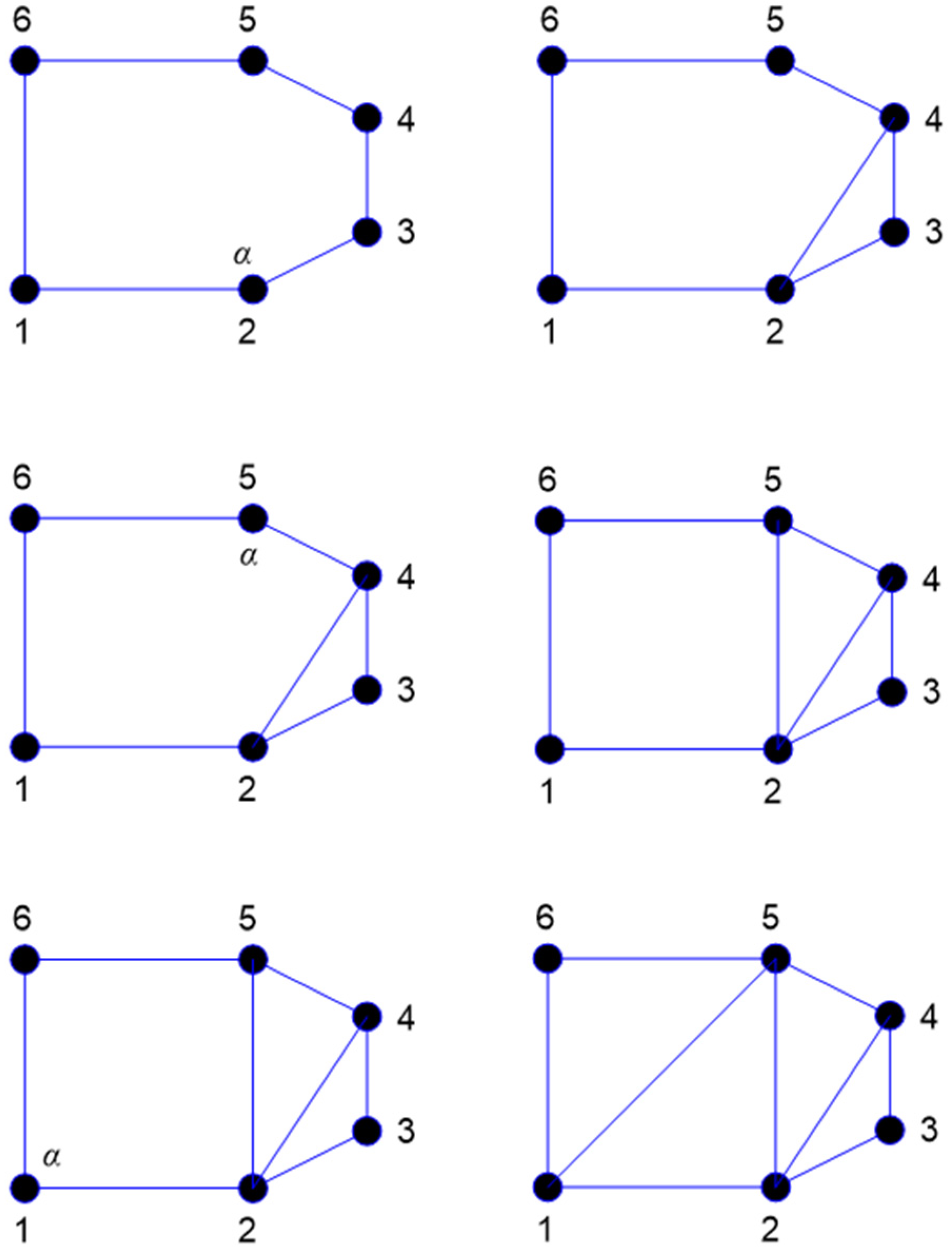
The dichotomy approach is used to construct the background mesh, which builds the mesh in a triangle form using all of the initial exterior boundary nodes of the figure. The computational space in this approach is represented as a polygon by continually splitting the computational domain into two subsets until the complete polygon subsets were created. Consequently, in order to connect any internal boundaries, including holes, to the external boundary, connecting lines must be constructed. The shortest path connecting all internal and external boundary points is used to construct the connection line [43]. Figure 2 displays the proposed method, which starts by separating each of the initial selected boundary sites with a large-faced angle and creating an angle set for selecting the nearest nonadjacent point to be linked with a new connected line. The face angle size is identified by the following precedence: $\pi \le {\theta }_1<2\pi , \pi /2<{\theta }_2<\pi , 0<{\theta }_3\le \pi /2.$

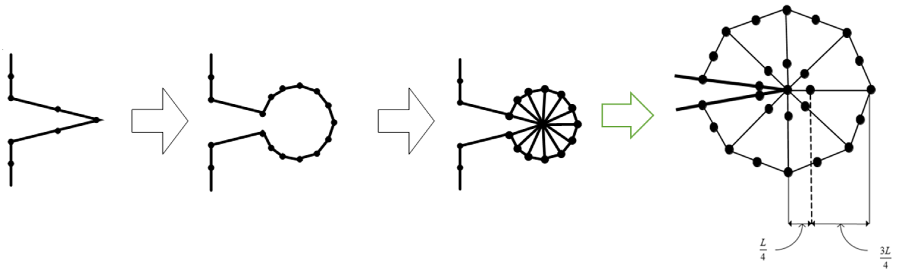
As a consequence, singular elements must be built to precisely characterize the singularity field at the crack front. Since the advancing front method [39] generates triangular elements from the faces of the boundaries, the area surrounding the crack front should be separated before generation of the singular elements. First, nodes are created surround the crack tip in a rosette manner, and then the node at the crack front and the related edge segments are extracted. Rosette elements are then constructed by forming triangles as seen in Figure 3.

2.3. Node Splitting and Relaxation

The release of nodes according to their mechanical properties is known as “relaxation of the split nodes”. There must be two independent nodes at a specific crack tip in order to mimic crack openings when the criterion for crack propagation is met. If the deformation is required to be shown, the displacement must be modified consistently using the border nodes’ coordinates. The node splitting and relaxation procedure was explained in detail in the previous study [5].

2.4. Refinement of the Adaptive Mesh

Finite element mesh optimization techniques include improving the adaptive mesh. Customized adaptive mesh refinement is first used to modify meshes all around the crack’s tip and along the crack itself. This method is dependent upon a posteriori error estimate from a prior mesh generation. It is possible to approximate the mesh refinement error quite well using the relative stress norm error. The h-type adaptive mesh refinement is used to estimate the ratio of the element standard stress error to the average area standard stress error. Each element’s mesh size is expressed in the following manner:

$$h_e=\sqrt{2A_e}$$

(4)

where A_e represents the element area. The following expression shows the average norm stress error over the entire domain:

$$\begin{array}{l}{\Vert \hat{\mathrm{e}}\Vert }^2=\frac{1}{m}{\displaystyle \sum _{e=1}^m{\displaystyle \underset{{\Omega }^e}{\int }{\sigma }^{\mathrm{T}}\sigma d\Omega }}\\ =\frac{1}{m}{\displaystyle \sum _{e=1}^m{\displaystyle \underset{{\Omega }^e}{\int }{\left\{\begin{array}{c}{\sigma }_x\\ {\sigma }_y\\ {\tau }_{xy}\\ {\sigma }_z\end{array}\right\}}^{\mathrm{T}}\left\{\begin{array}{c}{\sigma }_x\\ {\sigma }_y\\ {\tau }_{xy}\\ {\sigma }_z\end{array}\right\}d\Omega }}\end{array}$$

(5)

where m, represents the overall number elements. The Radau principle will modify the integration in the FEM’s triangular isoperimetric domain in the expression:

$$\begin{array}{l}{\Vert \mathrm{e}\Vert }_e^2 ={{\displaystyle \underset{-1}{\overset{1}{\int }}{\displaystyle \underset{-1}{\overset{1}{\int }}\left(\left\{\begin{array}{c}\sigma {\left(\xi ,\eta \right)}_x\\ \sigma {\left(\xi ,\eta \right)}_y\\ \tau {\left(\xi ,\eta \right)}_{xy}\\ \sigma {\left(\xi ,\eta \right)}_z\end{array}\right\}-\left\{\begin{array}{c}\sigma {\left(\xi ,\eta \right)}_x^{*}\\ \sigma {\left(\xi ,\eta \right)}_y^{*}\\ \tau {\left(\xi ,\eta \right)}_{xy}^{*}\\ \sigma {\left(\xi ,\eta \right)}_z^{*}\end{array}\right\}\right)}}}^{\mathrm{T}}\left(\left\{\begin{array}{c}\sigma {\left(\xi ,\eta \right)}_x\\ \sigma {\left(\xi ,\eta \right)}_y\\ \tau {\left(\xi ,\eta \right)}_{xy}\\ \sigma {\left(\xi ,\eta \right)}_z\end{array}\right\}-\left\{\begin{array}{c}\sigma {\left(\xi ,\eta \right)}_x^{*}\\ \sigma {\left(\xi ,\eta \right)}_y^{*}\\ \tau {\left(\xi ,\eta \right)}_{xy}^{*}\\ \sigma {\left(\xi ,\eta \right)}_z^{*}\end{array}\right\}\right)t^e\det J^{e}d\xi d\eta \\ ={{\displaystyle \sum _{p=1}^3\left(\left\{\begin{array}{c}\sigma {\left({\xi }_p,{\eta }_p\right)}_x\\ \sigma {\left({\xi }_p,{\eta }_p\right)}_y\\ \tau {\left({\xi }_p,{\eta }_p\right)}_{xy}\\ \sigma {\left({\xi }_p,{\eta }_p\right)}_z\end{array}\right\}-\left\{\begin{array}{c}\sigma {\left({\xi }_p,{\eta }_p\right)}_x^{*}\\ \sigma {\left({\xi }_p,{\eta }_p\right)}_y^{*}\\ \tau {\left({\xi }_p,{\eta }_p\right)}_{xy}^{*}\\ \sigma {\left({\xi }_p,{\eta }_p\right)}_z^{*}\end{array}\right\}\right)}}^{\mathrm{T}} \left(\left\{\begin{array}{c}\sigma {\left({\xi }_p,{\eta }_p\right)}_x\\ \sigma {\left({\xi }_p,{\eta }_p\right)}_y\\ \tau {\left({\xi }_p,{\eta }_p\right)}_{xy}\\ \sigma {\left({\xi }_p,{\eta }_p\right)}_z\end{array}\right\}-\left\{\begin{array}{c}\sigma {\left({\xi }_p,{\eta }_p\right)}_x^{*}\\ \sigma {\left({\xi }_p,{\eta }_p\right)}_y^{*}\\ \tau {\left({\xi }_p,{\eta }_p\right)}_{xy}^{*}\\ \sigma {\left({\xi }_p,{\eta }_p\right)}_z^{*}\end{array}\right\}\right)t^e\det J^e{W}_p\end{array}$$

(6)

and similarly

$${\Vert \hat{\mathrm{e}}\Vert }^2=\frac{1}{m}{\displaystyle \sum _{e=1}^m{{\displaystyle \sum _{p=1}^3\left(\left\{\begin{array}{c}\sigma {\left({\xi }_p,{\eta }_p\right)}_x\\ \sigma {\left({\xi }_p,{\eta }_p\right)}_y\\ \tau {\left({\xi }_p,{\eta }_p\right)}_{xy}\\ \sigma {\left({\xi }_p,{\eta }_p\right)}_z\end{array}\right\}\right)}}^{\mathrm{T}} \left(\left\{\begin{array}{c}\sigma {\left({\xi }_p,{\eta }_p\right)}_x\\ \sigma {\left({\xi }_p,{\eta }_p\right)}_y\\ \tau {\left({\xi }_p,{\eta }_p\right)}_{xy}\\ \sigma {\left({\xi }_p,{\eta }_p\right)}_z\end{array}\right\}\right)t^e\det J^e{W}_p}$$

(7)

where t^e is the element thickness for plane stress and t^e = 1 for plane strain. W_P is a weighting factor, and $J^e$ is the Jacobian matrix, which is expressed as:

$${\mathrm{J}}^e = \left[\begin{array}{cc}\frac{\partial x}{\partial \xi }& \frac{\partial y}{\partial \xi }\\ \frac{\partial x}{\partial \eta }& \frac{\partial y}{\partial \eta }\end{array}\right] = \left[\begin{array}{cc}{\displaystyle \sum _{i=1}^r\frac{\partial {\mathrm{N}}_i^e}{\partial \xi } x_i^e}& {\displaystyle \sum _{i=1}^r\frac{\partial {\mathrm{N}}_i^e}{\partial \xi } y_i^e}\\ {\displaystyle \sum _{i=1}^r\frac{\partial {\mathrm{N}}_i^e}{\partial \eta } x_i^e}& {\displaystyle \sum _{i=1}^r\frac{\partial {\mathrm{N}}_i^e}{\partial \eta } y_i^e}\end{array}\right]$$

(8)

As a result, each element’s relative stress norm error is substantially lower than 5%, which is within an acceptable range for a variety of engineering requirements [23]. Hence,

$${\zeta }_e=\frac{{\Vert e\Vert }_e}{\Vert \widehat{e}\Vert }\le \zeta$$

(9)

Therefore, the allowable error level for the new element is defined as:

$${\epsilon }_e=\frac{{\Vert e\Vert }_e}{\zeta \Vert \widehat{e}\Vert }\le 1$$

(10)

This means that more refinement must be applied to each element with ${\epsilon }_e>1$ using the asymptotic convergence rate criterion as follows:

$${\Vert e\Vert }_e\propto h_e^p$$

(11)

where p represents the estimation polynomial order. The new element size is calculated as follows for the quadratic polynomial:

$$h_N=\frac{1}{\sqrt{{\epsilon }_e}}{h}_e$$

(12)

Based on how many mesh refinements are specified, the previous mesh will then be reused as the proper background mesh, and this procedure will be repeated.

2.5. Displacement Extrapolation Method (DET)

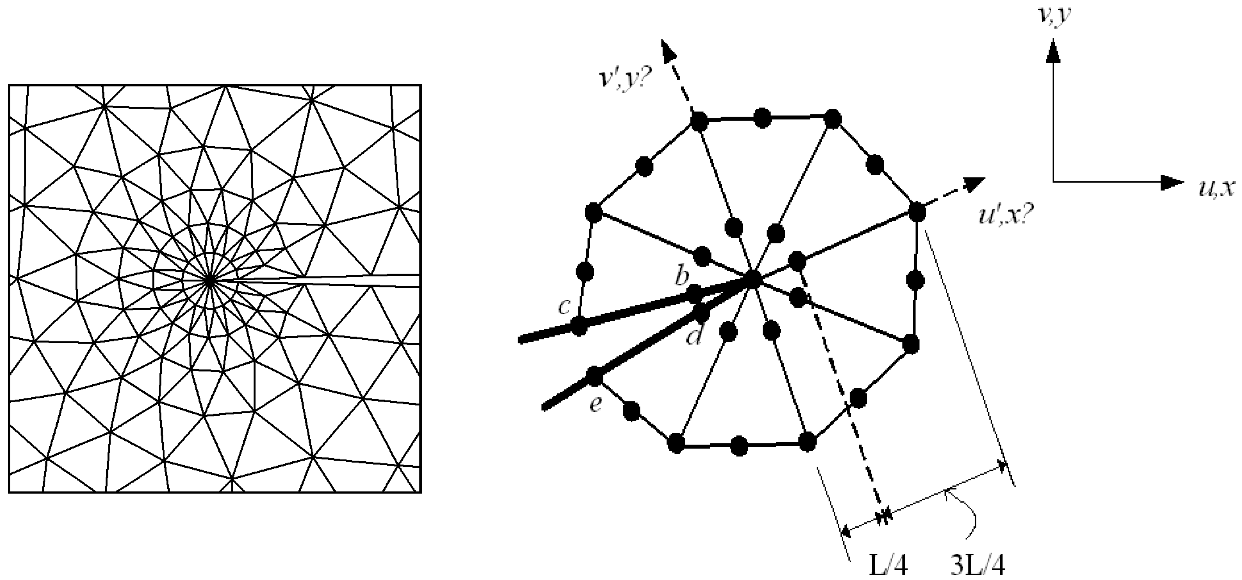
The SIFs for LEFM can be computed from the nodal displacement of finite elements using the displacement extrapolation technique. Three quarter-point singular elements surround the crack extremity in this technique, while six-node isoperimetric elements cover the remaining regions [42,43]. These partial nodes at the tip and along crack lines have their displacement components evaluated during extrapolation. The components’ SIFs are predicted using the necessary formulae. Using the displacement extrapolation technique, the rosette triangle components generated around the crack point are displayed in Figure 4.

The SIFs have been calculated using the following formulas [36]:

$$K_I=\frac{E}{3(1+v)(1+\kappa )}\sqrt{\frac{2\pi }{L}}\left[4({v^{\prime }}_b-{v^{\prime }}_d)-\frac{({v^{\prime }}_c-{v^{\prime }}_e)}{2}\right]$$

(13)

$$K_{II}=\frac{E}{3(1+v)(1+\kappa )}\sqrt{\frac{2\pi }{L}}\left[4({u^{\prime }}_b-{u^{\prime }}_d)-\frac{({u^{\prime }}_c-{u^{\prime }}_e)}{2}\right]$$

(14)

where E is the elasticity modulus, $v$ is the Poisson’s ratio, $\kappa$ is the elasticity factor represented as:

$$\kappa = \{\begin{array}{c}3-4v for plane strain\\ \frac{(3-v)}{(1+v)} for plane stress\end{array}$$

(15)

and L represents the quarter-point element length. Here, $u^{\prime }$ and $v^{\prime }$ are the two parameters of the displacement in x’ and y’, respectively, as shown in Figure 4.

3. Numerical Results and Discussions

3.1. A Rectangular Structure with Two Holes and One Central Crack

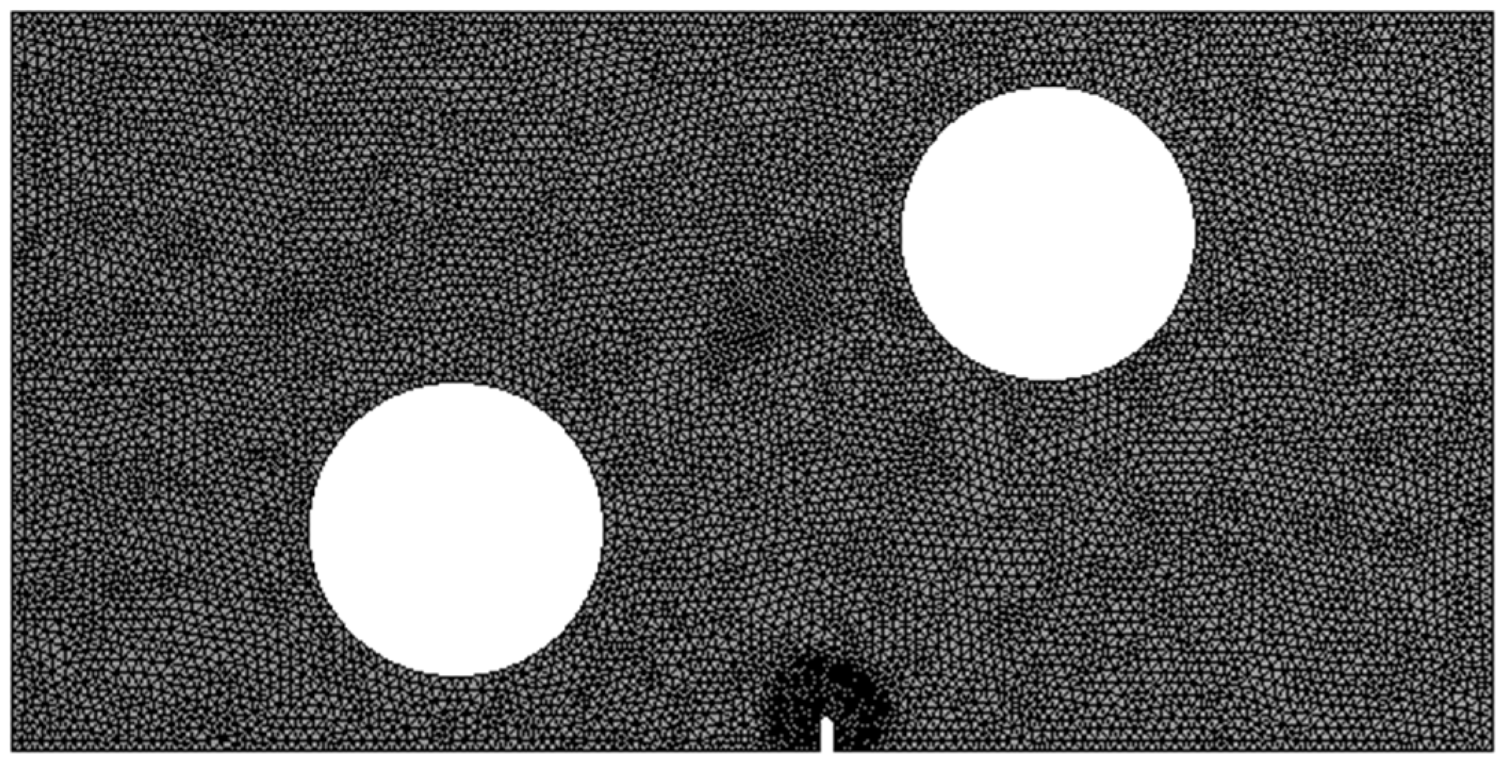
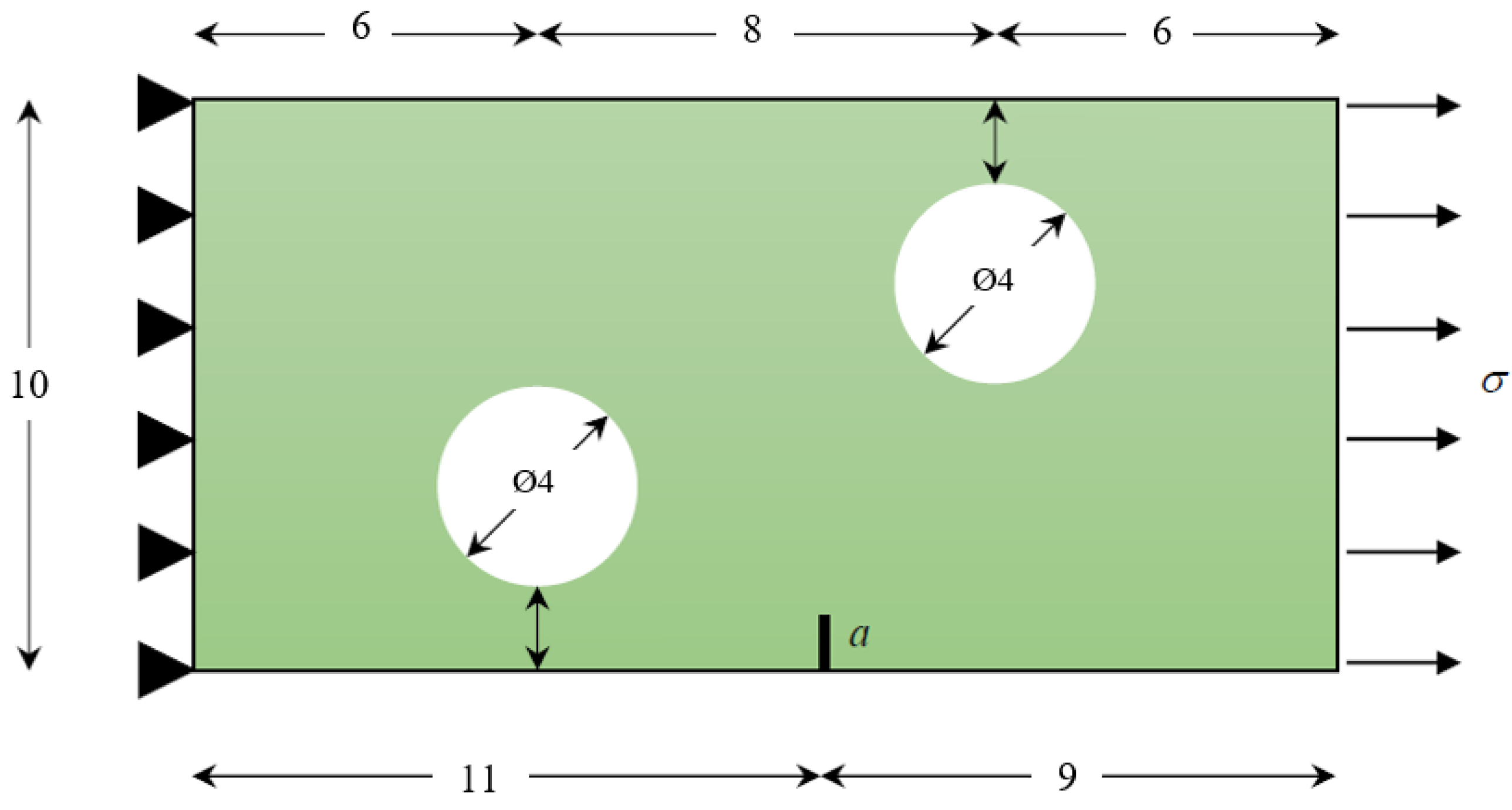
This example presents a rectangular structure with dimensions of 20 cm × 10 cm × 2 cm containing two holes with a diameter of 4 cm and one central crack with an initial crack length of 0.5 cm from the bottom, as depicted in Figure 5. The geometry is fixed from the left side, and the stress of 69 MPa is applied from the right edge. The material properties in the analysis are $E=69 \mathrm{GPa}$, $v=0.25$ and ${\sigma }_y=250 \mathrm{MPa}$. Figure 6 displays the initial adaptive mesh that was generated for this geometry, which includes a total of 104,729 elements and 132,270 nodes.

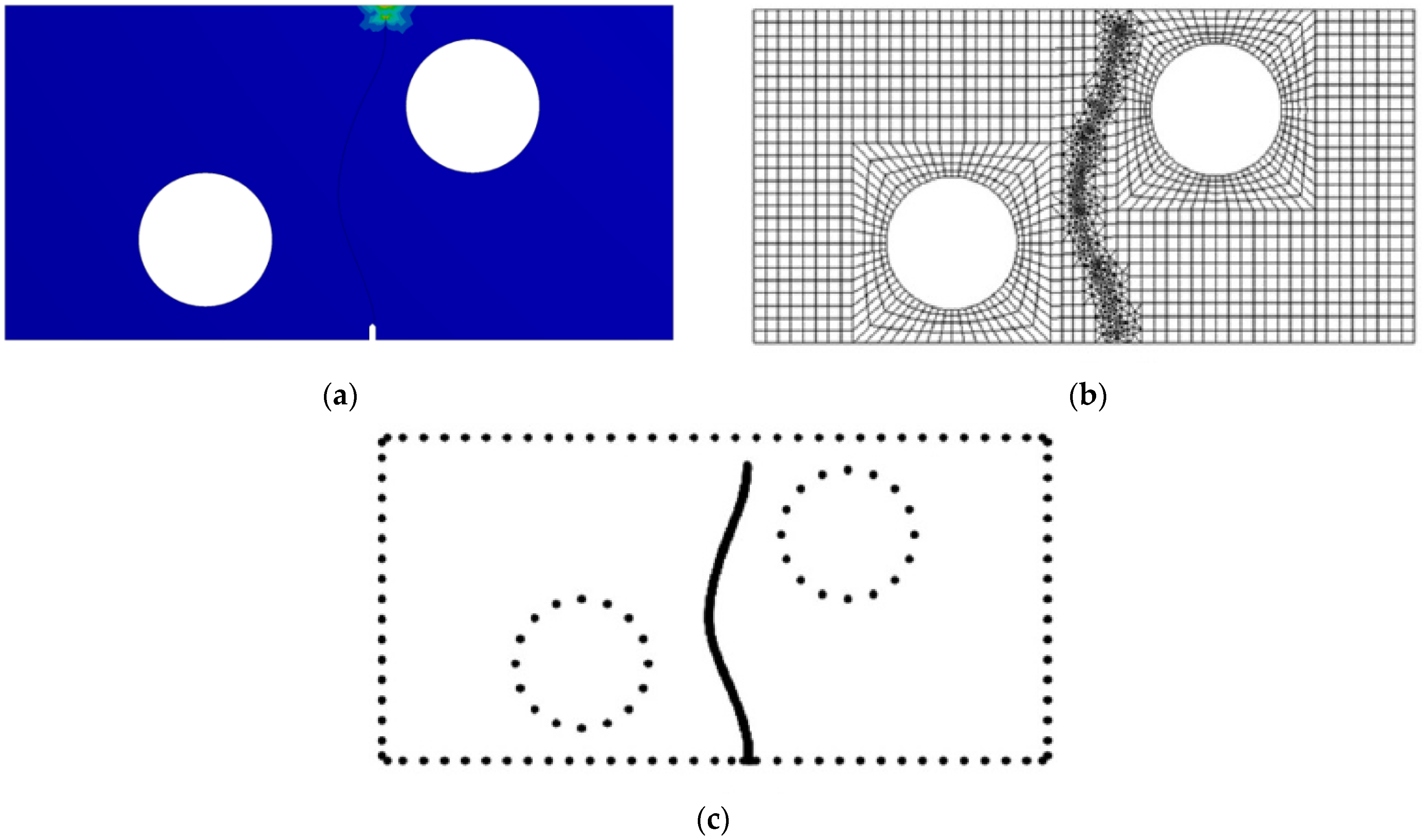
Figure 7 illustrates the comparison between the predicted crack propagation trajectory in the present study, the numerical results achieved by [44] using the dual boundary element method (DBEM), and the numerical results achieved using the Franc2D/L finite element program obtained by [45]. Firstly, the crack growth trajectory was completely dominated by the first mode of stress intensity factors, which propagated in a straight line. After that, the crack propagation trajectory was influenced by the lower hole and deviated slightly toward the hole, which was not close enough to attract the crack to sink into the hole. Consequently, the crack missed the hole and continued to propagate in a straight path once again. Lastly, the crack was influenced by the top hole and deviated slightly toward it, but again missed it since the hole was not close enough to draw the crack’s path into it.

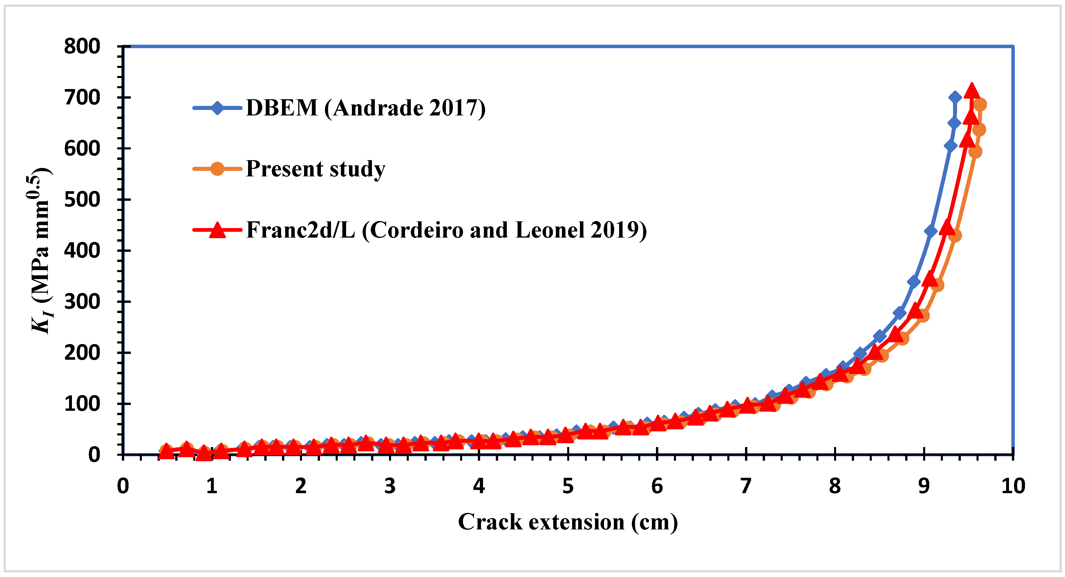
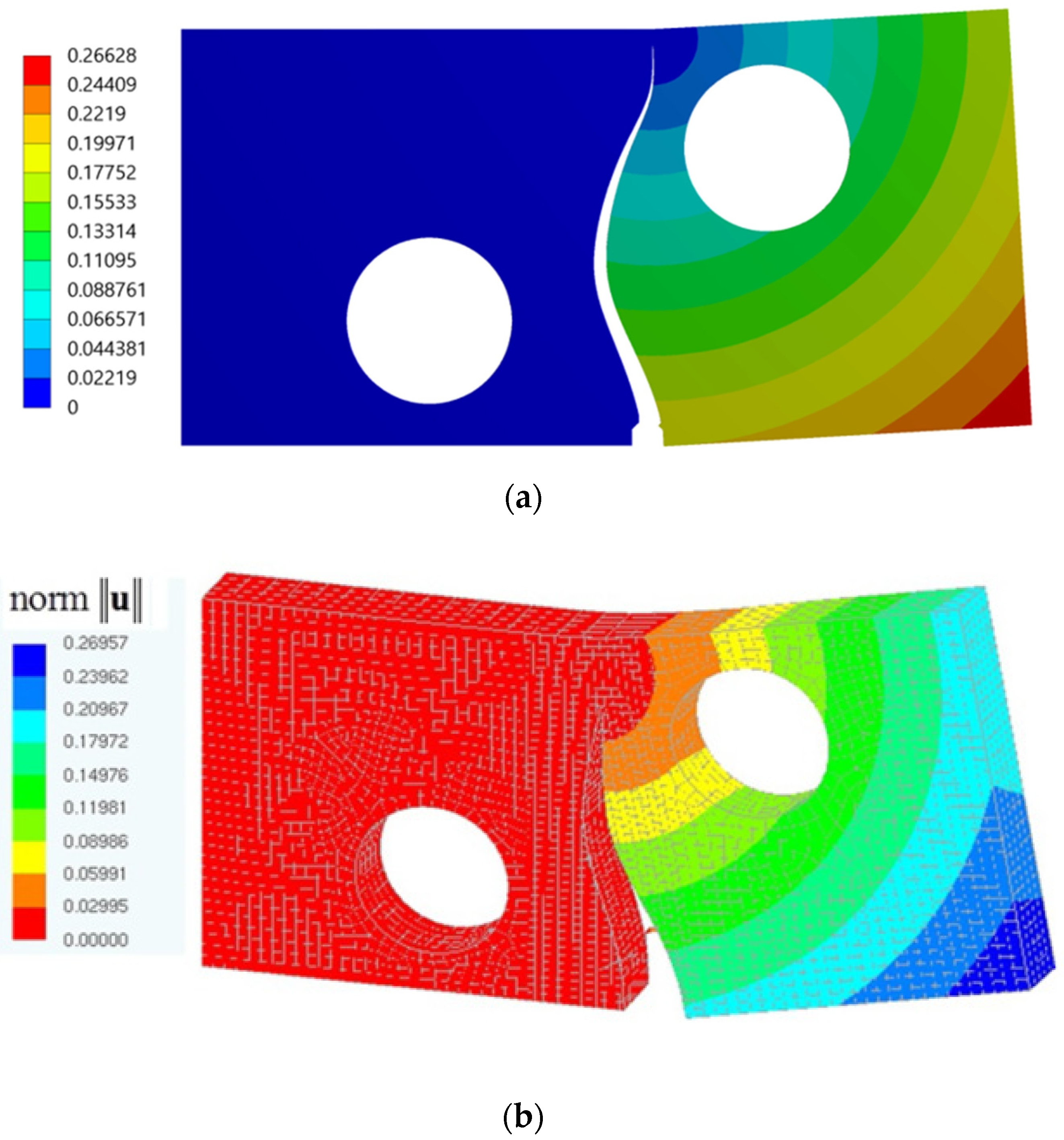
Figure 8 depicts the history of the first mode of stress intensity factors achieved by the developed program in comparison to the DBEM values and Franc2d/L proposed by [44,45], respectively. As can be seen in Figure 9, the final deformation that was obtained as the result of this study was similar to the deformation that had been predicted by [44] using a dual boundary element.

3.2. A Cracked Plate with Four Holes

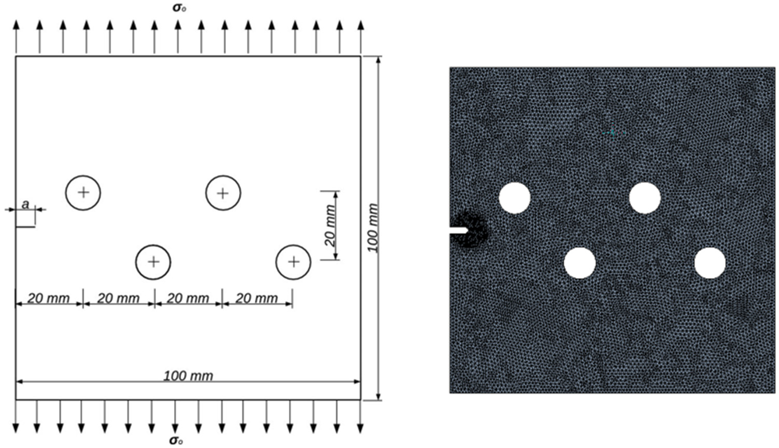
As depicted in Figure 10, we consider a square plate that has a single edge crack of 6 mm and four holes with identical radii of 5 mm each. The dimensions of the plate are 100 mm on each side and 10 mm in depth. The top and bottom edges are subjected to a uniformly distributed stress of 10 MPa. The properties of the plate, which is made of the aluminum alloy 7075-T6, are modulus of elasticity, E = 72 GPa, Poisson’s ratio, υ = 0.33, yield strength, σ_y = 469 MPa, ultimate strength, σ_u = 538 MPa, and fracture toughness, K_IC = 3288.76 MPa $\sqrt{mm}$.

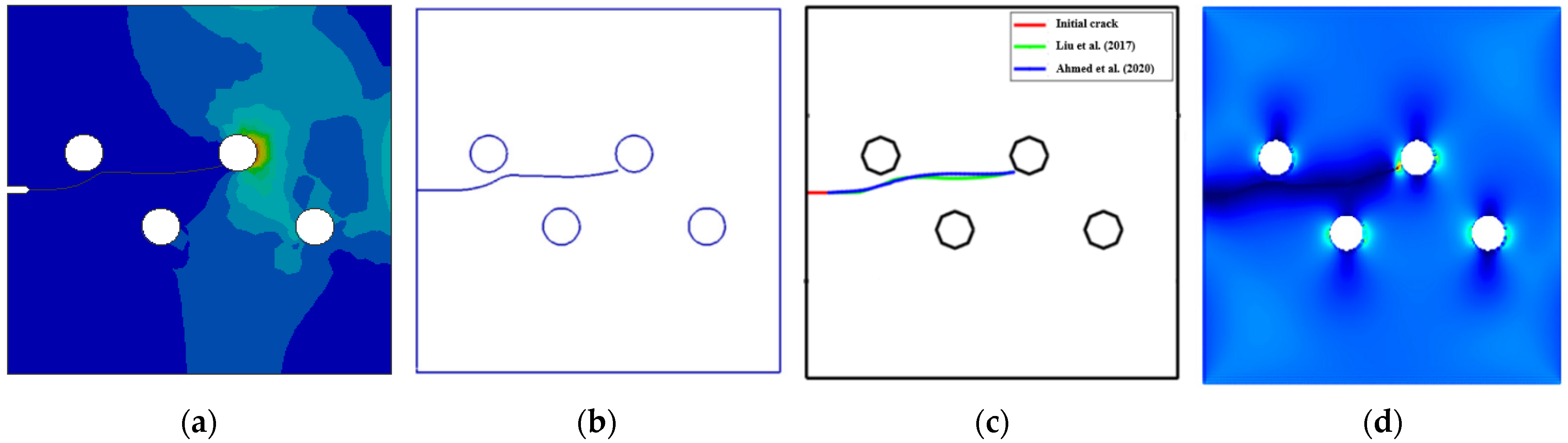
The predicted crack growth trajectory (Figure 11a) was in agreement with a variety of studies that used other ways of modeling, such as the fast multipole method (FMM) with the boundary element method (BEM) [46] (Figure 11b), the boundary cracklet method [47] (Figure 11c), and improved smoothed particle hydrodynamics [48] (Figure 11d). As seen in Figure 11d, there was a little divergence in the crack trajectory that was observed by Wiragunarsa et al. [48] when compared to the path that was predicted by the developed program and the two crack propagation paths that were addressed by [46,47].

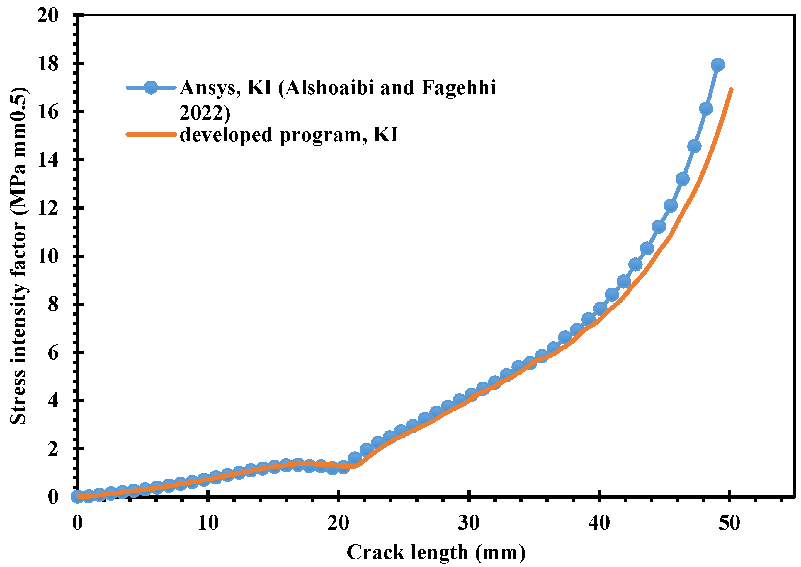
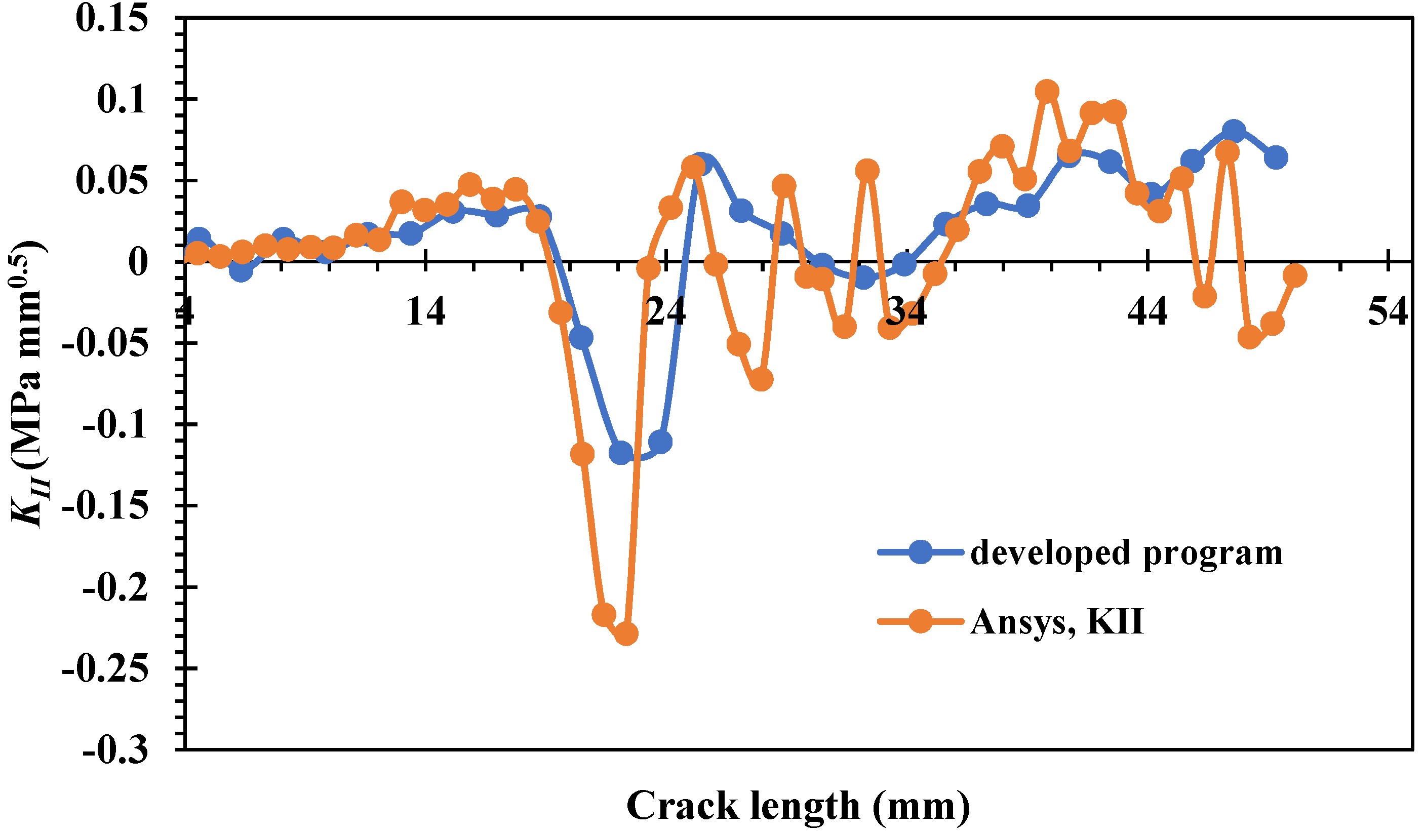
Figure 11 shows that, at first, the crack moves straight forward until it nears the first upper hole. At that point, the crack starts moving toward the hole. Subsequently, the crack is diverted in a different direction due to the fact that the first upper hole is not located in sufficient proximity to draw the crack into it. The crack eventually keeps moving forward in a straight line until it comes near enough to the second upper hole to sink into that hole. Figure 12 and Figure 13 show that the estimated values of the mixed-mode SIFs, K_I and K_II, have great agreement with the expected values achieved using the Ansys program [6]. The developed program results were nearly identical to the Ansys results, with a 0.4–5% deviation. Figure 12 and Figure 13 illustrate very clearly how the effect of the first upper hole on the crack growth path was represented in the curvature that was seen after 20 mm and how it disappeared after passing from the influence of this hole. This effect can be seen in the curvature that was seen after 20 mm in both figures.

4. Conclusions

In this study, two-dimensional crack growth on a rectangular structure with two holes and one central crack and on a cracked plate with four holes was studied using the developed FE source code program. The following results have been concluded from this work:

• These examples addressed a variety of issues, including the effect of hole location on the crack-growth trajectory, mixed-mode stress intensity factors, and stress distribution.
• The adaptive mesh structure was constructed using the advancing-front method, and the singularity was demonstrated by constructing quarter-point single elements around the crack tip.
• The presence of a hole in close proximity to a crack that is propagating can cause the crack path to be changed.
• The computed SIFs are in good agreement with the reference solutions.
• The developed program can accurately simulate the crack growth of any two-dimensional linear elastic structural component, according to comparisons with several benchmark problems of crack propagation from the literature.

References

- Huynh, H.D.; Nguyen, M.N.; Cusatis, G.; Tanaka, S.; Bui, T.Q. A polygonal XFEM with new numerical integration for linear elastic fracture mechanics. Eng. Fract. Mech. 2019, 213, 241–263. [Google Scholar] [CrossRef]
- Surendran, M.; Natarajan, S.; Palani, G.; Bordas, S.P. Linear smoothed extended finite element method for fatigue crack growth simulations. Eng. Fract. Mech. 2019, 206, 551–564. [Google Scholar] [CrossRef]
- Rozumek, D.; Marciniak, Z.; Lesiuk, G.; Correia, J. Mixed mode I/II/III fatigue crack growth in S355 steel. Procedia Struct. Integr. 2017, 5, 896–903. [Google Scholar] [CrossRef]
- Belytschko, T.; Black, T. Elastic crack growth in finite elements with minimal remeshing. Int. J. Numer. Methods Eng. 1999, 45, 601–620. [Google Scholar] [CrossRef]
- Alshoaibi, A.M.; Fageehi, Y.A. 2D finite element simulation of mixed mode fatigue crack propagation for CTS specimen. J. Mater. Res. Technol. 2020, 9, 7850–7861. [Google Scholar] [CrossRef]
- Alshoaibi, A.M.; Fageehi, Y.A. Finite Element Simulation of a Crack Growth in the Presence of a Hole in the Vicinity of the Crack Trajectory. Materials 2022, 15, 363. [Google Scholar] [CrossRef]
- Alshoaibi, A.M.; Fageehi, Y.A. 3D modelling of fatigue crack growth and life predictions using ANSYS. Ain Shams Eng. J. 2022, 13, 101636. [Google Scholar] [CrossRef]
- Bashiri, A.H.; Alshoaibi, A.M. Adaptive Finite Element Prediction of Fatigue Life and Crack Path in 2D Structural Components. Metals 2020, 10, 1316. [Google Scholar] [CrossRef]
- Li, X.; Li, H.; Liu, L.; Liu, Y.; Ju, M.; Zhao, J. Investigating the crack initiation and propagation mechanism in brittle rocks using grain-based finite-discrete element method. Int. J. Rock Mech. Min. Sci. 2020, 127, 104219. [Google Scholar] [CrossRef]
- Leclerc, W.; Haddad, H.; Guessasma, M. On the suitability of a Discrete Element Method to simulate cracks initiation and propagation in heterogeneous media. Int. J. Solids Struct. 2017, 108, 98–114. [Google Scholar] [CrossRef]
- Shao, Y.; Duan, Q.; Qiu, S. Adaptive consistent element-free Galerkin method for phase-field model of brittle fracture. Comput. Mech. 2019, 64, 741–767. [Google Scholar] [CrossRef]
- Yuan, H.; Yu, T.; Bui, T.Q. Multi-patch local mesh refinement XIGA based on LR NURBS and Nitsche’s method for crack growth in complex cracked plates. Eng. Fract. Mech. 2021, 250, 107780. [Google Scholar] [CrossRef]
- Nejad, R.M.; Liu, Z. Analysis of fatigue crack growth under mixed-mode loading conditions for a pearlitic Grade 900A steel used in railway applications. Eng. Fract. Mech. 2021, 247, 107672. [Google Scholar] [CrossRef]
- Alshoaibi, A.M.; Fageehi, Y.A. Numerical Analysis of Fatigue Crack Growth Path and Life Predictions for Linear Elastic Material. Materials 2020, 13, 3380. [Google Scholar] [CrossRef]
- ANSYS. Academic Research Mechanical, Release 19.2, Help System. In Coupled Field Analysis Guide; ANSYS, Inc.: Canonsburg, PA, USA, 2020. [Google Scholar]
- Abaqus User Manual; Abacus Version 2019; Simulia Corp.: Providence, RI, USA, 2019.
- Lebaillif, D.; Recho, N. Brittle and ductile crack propagation using automatic finite element crack box technique. Eng. Fract. Mech. 2007, 74, 1810–1824. [Google Scholar] [CrossRef]
- Duflot, M.; Nguyen-Dang, H. Fatigue crack growth analysis by an enriched meshless method. J. Comput. Appl. Math. 2004, 168, 155–164. [Google Scholar] [CrossRef] [Green Version]
- Yan, X. Automated simulation of fatigue crack propagation for two-dimensional linear elastic fracture mechanics problems by boundary element method. Eng. Fract. Mech. 2007, 74, 2225–2246. [Google Scholar] [CrossRef]
- Zhao, T.; Zhang, J.; Jiang, Y. A study of fatigue crack growth of 7075-T651 aluminum alloy. Int. J. Fatigue 2008, 30, 1169–1180. [Google Scholar] [CrossRef]
- Tada, H.; Paris, P.C.; Irwin, G.R.; Tada, H. The Stress Analysis of Cracks Handbook; ASME Press: New York, NY, USA, 2000; Volume 130. [Google Scholar]
- Murakami, Y.; Keer, L. Stress intensity factors handbook, vol. 3. J. Appl. Mech. 1993, 60, 1063. [Google Scholar] [CrossRef] [Green Version]
- Al Laham, S.; Branch, S.I. Stress Intensity Factor and Limit Load Handbook; British Energy Generation Limited Gloucester: Barnwood, UK, 1998; Volume 3. [Google Scholar]
- Zhu, W.; Smith, D. On the use of displacement extrapolation to obtain crack tip singular stresses and stress intensity factors. Eng. Fract. Mech. 1995, 51, 391–400. [Google Scholar] [CrossRef]
- Guinea, G.V.; Planas, J.; Elices, M. KI evaluation by the displacement extrapolation technique. Eng. Fract. Mech. 2000, 66, 243–255. [Google Scholar] [CrossRef]
- Rice, J.R. A path independent integral and the approximate analysis of strain concentration by notches and cracks. J. Appl. Mech. 1968, 35, 379–386. [Google Scholar] [CrossRef] [Green Version]
- Courtin, S.; Gardin, C.; Bezine, G.; Hamouda, H.B.H. Advantages of the J-integral approach for calculating stress intensity factors when using the commercial finite element software ABAQUS. Eng. Fract. Mech. 2005, 72, 2174–2185. [Google Scholar] [CrossRef]
- Fageehi, Y.A.; Alshoaibi, A.M. Numerical simulation of mixed-mode fatigue crack growth for compact tension shear specimen. Adv. Mater. Sci. Eng. 2020, 2020, 5426831. [Google Scholar] [CrossRef] [Green Version]
- Alshoaibi, A.M.; Hadi, M.; Ariffin, A. Finite element simulation of fatigue life estimation and crack path prediction of two-dimensional structures components. HKIE Trans. 2008, 15, 1–6. [Google Scholar] [CrossRef]
- Alshoaibi, A.M.; Fageehi, Y.A. Adaptive Finite Element Model for Simulating Crack Growth in the Presence of Holes. Materials 2021, 14, 5224. [Google Scholar] [CrossRef] [PubMed]
- Alshoaibi, A.M.; Hadi, M.; Ariffin, A. Two-dimensional numerical estimation of stress intensity factors and crack propagation in linear elastic Analysis. Struct. Durab. Health Monit. 2007, 3, 15. [Google Scholar]
- Alshoaibi, A.M.; Almaghrabi, M. Development of efficient finite element software of crack propagation simulation using adaptive mesh strategy. Am. J. Appl. Sci. 2009, 6, 661–666. [Google Scholar] [CrossRef]
- Alshoaibi, A.M. Finite element procedures for the numerical simulation of fatigue crack propagation under mixed mode loading. Struct. Eng. Mech. 2010, 35, 283–299. [Google Scholar] [CrossRef]
- Alshoaibi, A.M. An Adaptive Finite Element Framework for Fatigue Crack Propagation under Constant Amplitude Loading. Int. J. Appl. Sci. Eng. 2015, 13, 261–270. [Google Scholar]
- Alshoaibi, A.M. A Two Dimensional Simulation of Crack Propagation using Adaptive Finite Element Analysis. J. Comput. Appl. Mech. 2018, 49, 335. [Google Scholar]
- Fageehi, Y.A.; Alshoaibi, A.M. Nonplanar Crack Growth Simulation of Multiple Cracks Using Finite Element Method. Adv. Mater. Sci. Eng. 2020, 2020, 8379695. [Google Scholar] [CrossRef] [Green Version]
- Alshoaibi, A.M.; Fageehi, Y.A. Simulation of Quasi-Static Crack Propagation by Adaptive Finite Element Method. Metals 2021, 11, 98. [Google Scholar] [CrossRef]
- Alshoaibi, A.M. Comprehensive comparisons of two and three dimensional numerical estimation of stress intensity factors and crack propagation in linear elastic analysis. Int. J. Integr. Eng. 2019, 11, 45–52. [Google Scholar] [CrossRef] [Green Version]
- Zienkiewicz, O.C.; Taylor, R.L.; Zhu, J.Z. The Finite Element Method: Its Basis and Fundamentals; Elsevier: Amsterdam, The Netherlands, 2005. [Google Scholar]
- Erdogan, F.; Sih, G. On the crack extension in plates under plane loading and transverse shear. J. Basic Eng. 1963, 85, 519–525. [Google Scholar] [CrossRef]
- Sun, C.; Jin, Z. Chapter 4—Energy Release Rate. In Fracture Mechanics, 1st ed.; Academic Press: Cambridge, MA, USA, 2012; pp. 77–103. [Google Scholar]
- Anderson, T.L. Fracture Mechanics: Fundamentals and Applications; CRC Press: Boca Raton, FL, USA, 2017. [Google Scholar]
- Sezer, L.; Zeid, I. Automatic quadrilateral/triangular free—Form mesh generation for planar regions. Int. J. Numer. Methods Eng. 1991, 32, 1441–1483. [Google Scholar] [CrossRef]
- Andrade, H.D.C. Análise da Propagação de Fissuras em Estruturas Bidimensionais Não-Homogêneas via Método dos Elementos de Contorno; Universidade de São Paulo: São Paulo, Brazil, 2017. [Google Scholar]
- Cordeiro, S.G.F.; Leonel, E.D. An improved computational framework based on the dual boundary element method for three-dimensional mixed-mode crack propagation analyses. Adv. Eng. Softw. 2019, 135, 102689. [Google Scholar] [CrossRef]
- Liu, Y.; Li, Y.; Xie, W. Modeling of multiple crack propagation in 2-D elastic solids by the fast multipole boundary element method. Eng. Fract. Mech. 2017, 172, 1–16. [Google Scholar] [CrossRef]
- Ahmed, T.; Yavuz, A.; Turkmen, H.S. Fatigue crack growth simulation of interacting multiple cracks in perforated plates with multiple holes using boundary cracklet method. Fatigue Fract. Eng. Mater. Struct. 2021, 44, 333–348. [Google Scholar] [CrossRef]
- Wiragunarsa, I.M.; Zuhal, L.R.; Dirgantara, T.; Putra, I.S. A particle interaction-based crack model using an improved smoothed particle hydrodynamics for fatigue crack growth simulations. Int. J. Fract. 2021, 229, 229–244. [Google Scholar] [CrossRef]
Figure 1.
Program flowchart.
Figure 2.
Polygon division using the proposed dichotomy approach.
Figure 3.
Special quarter-point finite elements at a crack front.
Figure 4.
Elements and coordinates of a triangular rosette at the crack front.
Figure 5.
Geometrical representation of the rectangular structure with two holes and one central crack.
Figure 6.
Initial adaptive mesh of the rectangular structure with two holes and one central crack.
Figure 7.
Crack growth path (a) present study, (b) dual boundary element method [44], and (c) FEM with Franc2d/L [45].
Figure 9.
Total deformation of the last step of crack propagation (a) present study, (b) DBEM by [44].
Figure 10.
Geometrical dimensions (left) and its initial adaptive mesh (right).
Figure 11.
Crack propagation paths: (a) present study, (b) Liu et al. FMM BEM [46], (c) Ahmed et al. [47], and (d) Wiragunarsa et al. [48].
Figure 12.
Predicted values of the KI in comparison to Ansys results obtained by [6].
Figure 13.
Predicted values of the KII in comparison to Ansys results obtained by [6].
Disclaimer/Publisher’s Note: The statements, opinions and data contained in all publications are solely those of the individual author(s) and contributor(s) and not of MDPI and/or the editor(s). MDPI and/or the editor(s) disclaim responsibility for any injury to people or property resulting from any ideas, methods, instructions or products referred to in the content. |
© 2022 by the authors. Licensee MDPI, Basel, Switzerland. This article is an open access article distributed under the terms and conditions of the Creative Commons Attribution (CC BY) license (https://creativecommons.org/licenses/by/4.0/).
Share and Cite
MDPI and ACS Style
Alshoaibi, A.M.; Fageehi, Y.A. A Computational Framework for 2D Crack Growth Based on the Adaptive Finite Element Method. Appl. Sci. 2023, 13, 284. https://doi.org/10.3390/app13010284
AMA Style
Alshoaibi AM, Fageehi YA. A Computational Framework for 2D Crack Growth Based on the Adaptive Finite Element Method. Applied Sciences. 2023; 13(1):284. https://doi.org/10.3390/app13010284
Chicago/Turabian StyleAlshoaibi, Abdulnaser M., and Yahya Ali Fageehi. 2023. "A Computational Framework for 2D Crack Growth Based on the Adaptive Finite Element Method" Applied Sciences 13, no. 1: 284. https://doi.org/10.3390/app13010284
Note that from the first issue of 2016, this journal uses article numbers instead of page numbers. See further details here.