Design Framework for Selection of Grid Topology and Rectangular Cross-Section Size of Elastic Timber Gridshells Using Genetic Optimisation

Abstract

This work presents a design framework for the selection of the topology and cross-section size of elastic timber gridshells, taking as constraints the shape of the structure and the maximum value of bending stress that can be reached in a given area of the gridshell. For this purpose, a parametric design environment and a genetic optimisation algorithm are used, which provides a set of solutions (optimal and near-optimal) that can be examined by the designer before adopting the final solution. The construction of the parametric mesh model is based on a geometric approach using an original adaptation of the Compass Method by developing two algorithms. The first one plots geodesic curves on a surface given a starting point and a direction. The second algorithm adapts the accuracy of the Compass Method to the local curvature of the surface, substantially minimising the computation time. The results show that the optimisation process succeeds in significantly reducing the initial bending stresses and offers an interesting solution space, consisting of a set of solutions with sufficiently diverse topologies and cross-section sizes, from which the final solution can be chosen by the Decision Maker, even according to additional non-programmed structural or aesthetic requirements. The design framework has been successfully applied and verified in the design of the PEMADE gridshell, an innovative elastic timber gridshell recently realised by the authors. Finally, the most relevant details of its construction process carried out to ensure the exact position of the timber laths are presented.

1. Introduction

Gridshells are a highly efficient and architecturally expressive structural solution of great interest for their application in lightweight roofs of medium and large spans. They have recently gained increasing relevance due to their reduced use of material and the resulting environmental benefits [1]. Elastic timber gridshells are built from initially straight timber laths of small cross-section and long length, which are elastically deformed until they reach the target shape, creating a structural grid of continuous elements. Although structures built using this procedure were originally called gridshells [2], they are now often referred to as elastic gridshells [3], bending active gridshells [4], or strained gridshells [5] to differentiate them from other gridshell structures whose laths are not elastically curved.

The use of timber laths of identical cross-section and simple connection solutions make the system highly prefabricated and standardisable, with great potential for common applications such as sports, commercial, cultural, industrial, or agricultural buildings [6]. However, only a few works with this type of structure have been carried out. This is due to major difficulties during the design and construction process that prevent their popularisation, such as the shortage of suitable commercial timber products [7], insufficient studies on stress relaxation in curved timber laths [8], and the lack of research on experimentally tested numerical models [9].

The construction process for elastic timber gridshells involves significant deformations of the laths. These deformations lead to high stresses (bending, torsion, shear, and normal), with the bending stress the most critical [9,10]. The bending stresses caused by curving the laths depend on the laths’ cross-section and material, as well as on the geometry of the grid (surface curvature and orientation of the laths over it). Obviously, these stresses must be lower than the strength of the material, while keeping a sufficient structural reserve to resist the stresses caused by the external loads and considering rheological phenomena. The solution to avoid high bending stresses is to use sufficiently large curvature radii or very small lath thicknesses. Both strategies imply a reduction in bending stiffness perpendicular to the plane of the structure. This is an inherent contradiction of elastic timber gridshells, which generally require an iterative sizing process. Consequently, it is necessary to have some procedure to generate the grid and evaluate the bending stresses from the preliminary design stages to ensure appropriate values. This is one of the main challenges in the design of elastic timber gridshells.

In traditional elastic timber gridshells, two types of mesh have been used to generate the grid: the geodesic meshes in the ribbed shells of J. Natterer [11], and the constant-sided quadrangular meshes in the gridshells of F. Otto [2]. Geodesic meshes have the advantage that laths are subjected to bending only about their weak axis, but the disadvantage that the distance between nodes is variable on free-form surfaces, which can cause the grid to have an irregular appearance. In contrast, quadrangular grids keep a constant distance between nodes, offering a more regular pattern for any surface, but have the disadvantage that the laths are subjected to bending about both weak and strong axes.

In elastic timber gridshells for building construction, the general problem to be solved is usually to determine the grid geometry on an imposed architectural surface, which has been approached in different ways. In recent years, several research studies have focused on the dynamic relaxation method with kinetic damping for gridshell form-finding thanks to its suitability for non-linear systems with large displacements [12,13,14,15]. This approach determines the deformed grid geometry on an imposed architectural surface by relaxation [16,17] and can be applied for both geodesic and quadrangular meshes.

Another very different approach lies in the use of geometric methods rather than mechanical simulations. In this regard, the Compass Method (CM) described in [2] has been applied for the generation of quadrangular meshes in the design of gridshells made of timber [18] and other materials [19]. However, this approach has the drawback of requiring the definition of two random initial (master) curves over the surface, whose position and shape have a major impact on the resulting mesh. In addition, the CM shows dimensional accuracy errors when the target surface has high local curvature. This drawback can be overcome by applying the Improved Compass Method (ICM) [20] but doing so requires a significant increase in computational time.

In elastic gridshells, the stresses due to the construction process are the most important loads [9,10], so minimising the initial stresses due to bending for a given cross-section is always a desirable objective that depends exclusively on the material and the grid geometry. Genetic algorithms (GAs) have been developed especially in the last two decades [21] and have been applied successfully to solve structural optimisation problems. The development of such optimisation algorithms is analogous to evolutionary theory, as the individuals generated in the solution space after each generation evolve in a kind of natural selection, and have been widely described in the last decades [22]. This natural selection is performed by measuring how fit each individual in a population is by testing how high its score is against a predefined fitness function (FF). The fitter the individual is, the more likely it is to pass on its genes to its offspring for the next generation. The optimal solution is found after a recursive evolution of a population of individuals or chromosomes (solution vectors or parameters in the solution space) until the optimality criterion is reached [23] or no improvement is achieved. In this evolutionary process, stronger or fitter individuals (higher score value from the FF) have more chances to pass their genes (variable parameters or components of a solution vector) to the next generation of individuals by means of reproduction, combining the parents’ genes through gene crossover. During evolution, mutation may occur, introducing random diversity in the population and preventing local optima convergence [24]. The weaker or unfit individuals in each generation should be extinguished by natural selection and are dismissed by the algorithm. On the contrary, if the offspring are strong, they should endure, evolving the species. Existing GAs differ in the method of introducing diversity into solutions and in how they promote and maintain the best-fit individuals from one generation to the next [25]. Much research has been conducted to determine the best-performing GAs, concluding that elitist algorithms are the most efficient for most optimisation problems [26].

Generative design environments coupled with single-objective or multi-objective optimisation GAs have been widely and successfully applied to the design of gridshells, in most cases taking form-finding, topology, and/or structural performance as objectives [27,28,29]. GAs have also been successfully applied to the design of elastic gridshells made of circular cross-section composites [30]. In this case, the initial bending stresses were minimised indirectly by minimising the grid curvatures and considering the diameter of the tubes as a starting assumption.

In the case of elastic timber gridshells, it is not common to know the cross-section size at the beginning of the design, so the choice of a cross-section is also part of the problem. Furthermore, in free-edge elastic timber gridshells, such as the PEMADE gridshell (Figure 1) recently designed by the authors [31], there are other constructional or aesthetic issues, such as the distances from the ends of the laths to the nearest grid intersection (end distances), which strongly influence the design decision-making process and are not necessarily programmable. This is a non-deterministic design process that requires the analysis of a large number of valid near-optimal solutions to choose from. In this sense, the use of GAs algorithms represents the perfect tool to generate a solution scape automatically while trying to optimise some features of the design of elastic timber gridshells.

This paper presents a framework for the design of elastic timber gridshells with a quadrangular mesh. Specifically, a procedure is presented for the choice of cross-section size and grid topology for the usual case in which the surface is imposed. For this purpose, a generative design environment is used, coupling a parametric mesh model with a genetic optimisation algorithm (Strong Pareto Evolutionary Algorithm 2). The construction of the parametric mesh model is based on a geometric approach using an original adaptation of the CM, called an Adaptative Compass Method (ACM) in this work, which adapts the accuracy of the CM to the local curvature of the surface. The accuracy gains with respect to the CM and the reduction of computation time with respect to the ICM are analysed. Geodesic curves are proposed as master curves for the ACM. A new algorithm for plotting them from a starting point and a direction is also presented. The proposed design framework has been successfully applied and verified in the design of the PEMADE gridshell. In addition, the most important details of its construction are presented, which have made it possible to guarantee the execution of the finally chosen grid.

2. Design Process

This section presents an overview of the design process proposed in this work, which is carried out in two steps composed of three phases each: (1) Parametric model; (2) Optimisation; and (3) Decision making. The three phases are executed in a very similar way in the two steps. The following Sections (Section 3, Section 4 and Section 5) detail the method or procedure followed in each of them. The proposed design process requires establishing an initial set of available cross-section sizes and the maximum value of the bending stress that can be reached due to the curving process in a given area of the structure.

In Step 1, the size of the cross-sections for which the defined maximum stress is not exceeded is obtained. In addition, this first set of solutions provides a first approximation of the minimum value of the maximum initial bending stress that can be reached for each cross-section size, as well as the improvement achieved with the optimisation process.

In Step 2, once the final cross-section size is chosen, a new set of topologic configurations is obtained in which the maximum bending stress value is minimal (or near-minimal). This set of solutions provides a decision space in which other non-programmed or not-programmable issues, such as end distances or other aesthetic considerations, can be taken into account.

The main aspects of each of the above-mentioned phases are summarised below:

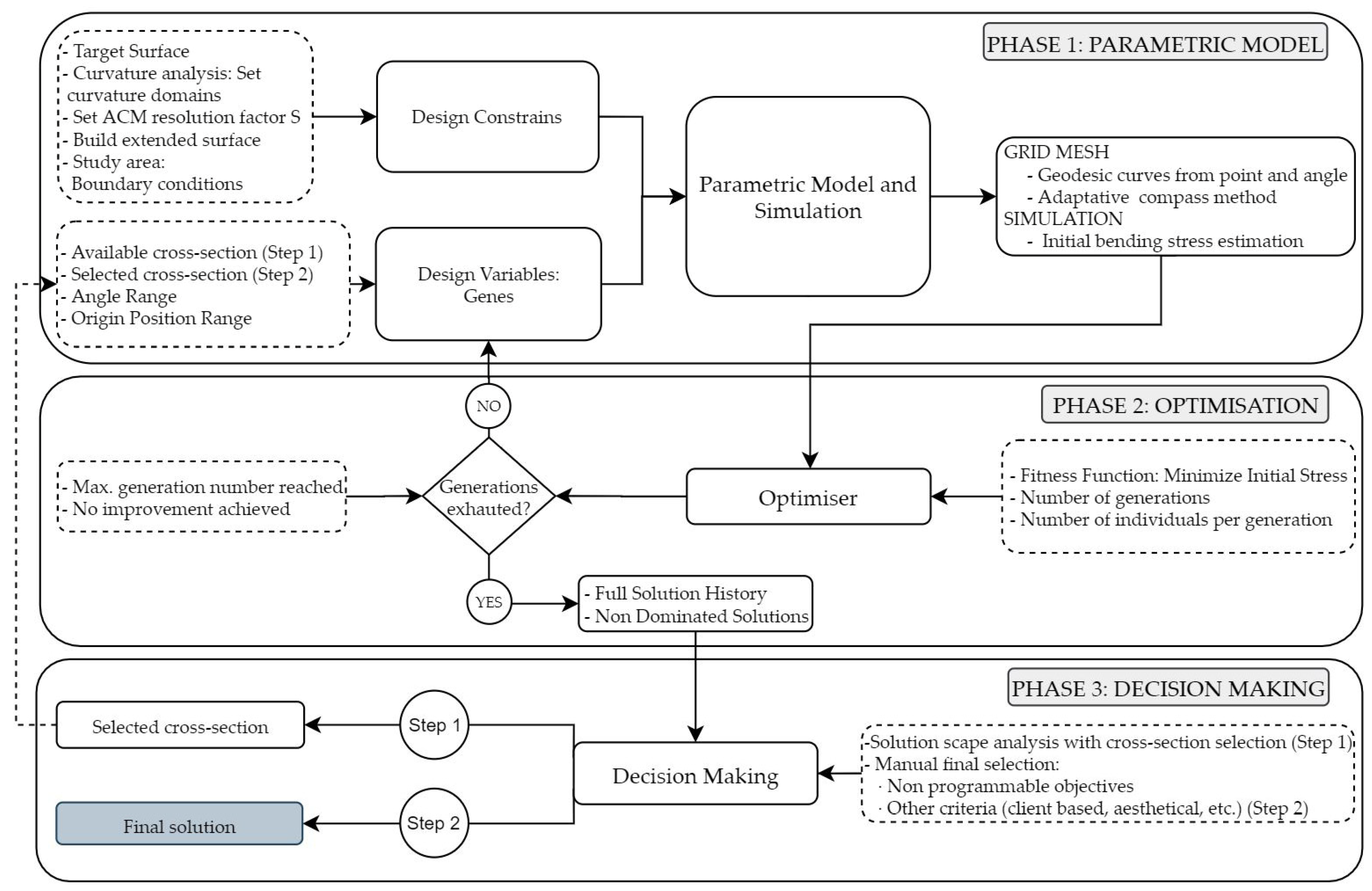
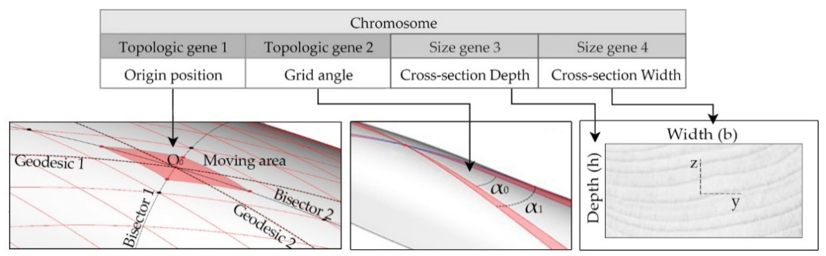
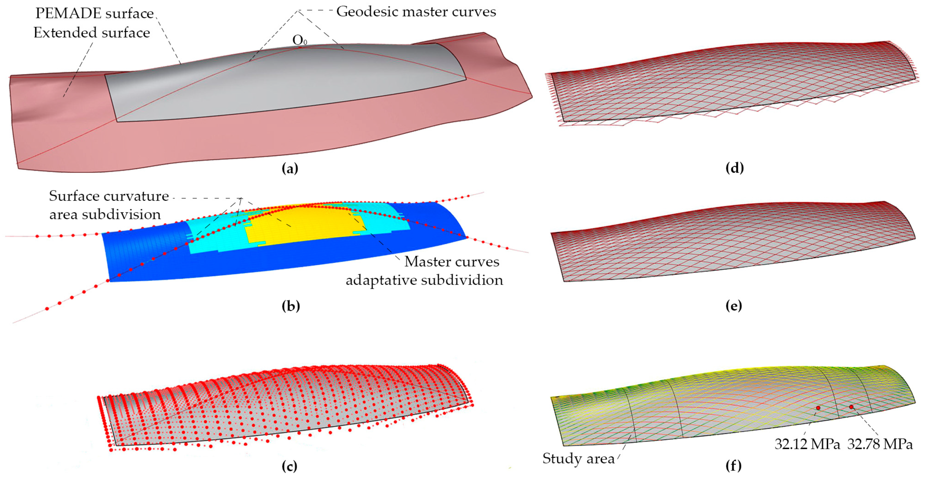
• Phase 1: Parametric model. In this initial phase, the parametric model is built according to the procedure described in Section 3, considering as design constraints the target surface and the study area. The target surface is an external and fixed customer input. The study area is the surface portion where the initial bending stresses are intended to be minimised. It may coincide with the entire target surface, but in general it is of interest to restrict it only to the area of the grid where the highest bending stresses due to external loads (dead loads, snow, wind, etc.) will occur. Next, the parametric model of the gridshell logic considers the design variables that will define its topology and the cross-section size of the laths, which constitute the genes of the optimisation algorithm. In Step 1, the genes are the topological variables (the origin position of the geodesic curves and the grid angle) and the cross-section size variables (depth and width). In Step 2, once the final cross-section is chosen, the genes are the topological variables only. The parametric model will be able to mesh the surface starting from a pair of geodesic curves calculated from a starting point and an angle, and to fill the surface with a full mesh by running the algorithms for geodesic curves and the ACM. To establish the ACM parameters, the algorithm first analyses the curvature of the target surface, allocating the subdivision domains according to the curvature and assigning the resolution factor S. Once the parametric model is built, simulations can be run by estimating the initial bending stress both in the study area, where its minimisation will be required, and in the entire grid to verify that the predefined maximum stress is not exceeded at any point, for each individual valid solution.
• Phase 2: Optimisation. The algorithm performs the optimisation routine based on the Strong Pareto Evolutionary Algorithm 2 (SPEA-2) fed with the data obtained from the parametric model for each generation. It is driven by the minimisation of a fitness function defined later on. As long as the number of generations is below the prescribed maximum and the optimisation process is still in progress, the algorithm loops back to the parametric model, tuning the genes as necessary for optimisation purposes. This phase is detailed in Section 4.
• Phase 3: Decision making. In this final phase detailed in Section 5, the Decision Maker (DM) analyses the solution scape, imposes further requirements and selects the final solution. In Step 1, the range of cross-sections that meet the condition that the maximum bending stress does not exceed the established limit stress is obtained. The DM selects the final cross-section size based on criteria such as the required minimum cross-section width (which may be determined by the diameter of the dowel-type fastener), the cross-sections available in the sawmill, or others. The selected cross-section depth and width are used as fixed input data for the parametric model in Step 2, where a set of mesh solutions varying the topological genes is obtained, in which the maximum initial bending stresses are minimal and near-minimal. Among them, the DM can choose the final solution based not only on mechanical criteria, but also on other non-programmed structural criteria, such as the minimum distances from the connections to the end of the laths or aesthetic issues. Moreover, the DM does not necessarily have to be the engineer performing this method but may be the architect in charge of the final design or even the client who could take into account, for example, aesthetical criteria, among other subjective aspects.

The workflow diagram of the proposed design process is shown in Figure 2. Most elements of the three phases are common to both steps. Where this is not the case, the corresponding step is indicated in the text.

3. Parametric Model Definition

This section describes the main aspects of the parametric model developed for the generation of a quadrangular mesh with a constant distance between nodes on a given surface. The procedure applies a geometric approach based on an original adaptation of the Compass Method, using two geodesic curves as master curves, and adapting the discretisation size of the Compass Method to the local curvature of the surface to be meshed in order to reduce the dimensional error and the computational time. The description of the proposed algorithms is completed with a review of the fundamental geometrical concepts and a summary of the most relevant background. Finally, the procedure followed for the evaluation of the bending stresses due to the bending process of the laths is described.

3.1. Surface Meshing Method

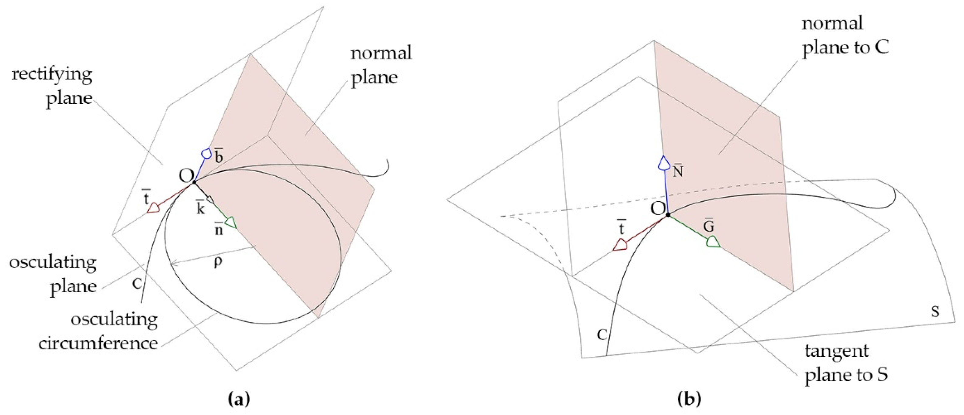
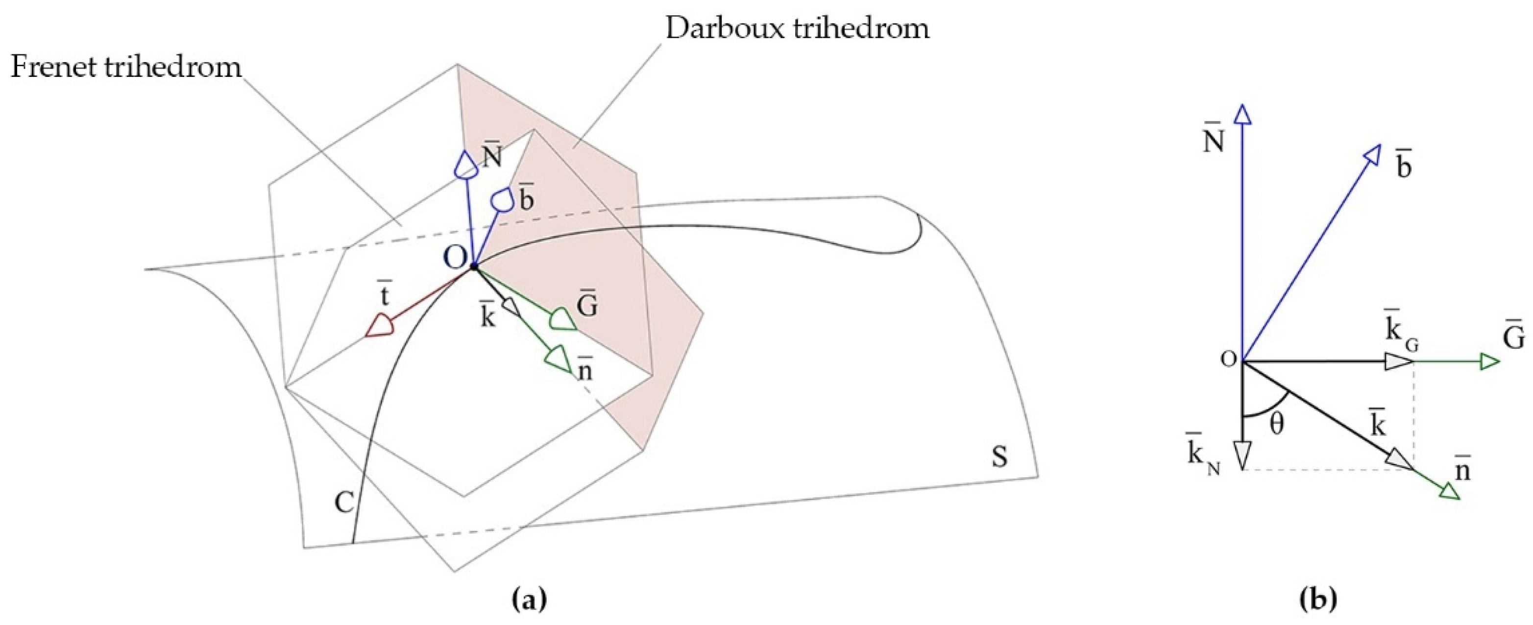
3.1.1. Generation of Geodesic Master Curves: Geometrical Fundamentals

On any curve C in space, an intrinsic trihedron can be defined along the curve, known as the Frenet trihedron. At any point O on the curve, this trihedron is defined by the vector $\overrightarrow{t}$ tangent to the curve at the point, the normal vector $\overrightarrow{n}$ (unit vector of the curvature vector $\overrightarrow{k}$), and the binormal vector $\overrightarrow{b}$ (cross product of the tangent and curvature vectors). The line normal to the curve at a point contains the vectors $\overrightarrow{n}$ and $\overrightarrow{k}$ and the centre of curvature of the curve at that point. At each point on the curve, the circumference with a centre at the centre of curvature and with the same radius of curvature as the curve is called the osculating circumference and is contained in the plane formed by the vectors $\overrightarrow{n}$ and $\overrightarrow{t}$.

At the same point O of the curve, but now contained in a surface S, there is a trihedron of the curve associated with the surface called a Darboux trihedron, which is defined by the vector $\overrightarrow{t}$ tangent to the curve and the surface, a vector $\overrightarrow{N}$ normal to the surface, and the geodesic vector $\overrightarrow{G}$.

Figure 3 shows the Frenet and Darboux trihedrons at a point O on curve C. It can be observed that the planes defined by the vectors $\overrightarrow{N}$ and $\overrightarrow{G}$, and $\overrightarrow{n}$ and $\overrightarrow{b}$ (planes marked in red) are coplanar since both are perpendicular to the vector $\overrightarrow{t}$.

Figure 4 shows the relationship between the Frenet and Darboux trihedron vectors projected onto any of the coplanar planes mentioned above and the components of the curvature vector $\overrightarrow{k}$.

The curvature vector $\overrightarrow{k}$ indicates the curvature of the curve in space at point O. The curvature of the curve on the surface can be evaluated by projecting the vector $\overrightarrow{k}$ onto the vectors $\overrightarrow{N}$ and $\overrightarrow{G}$ of the Darboux trihedron and obtaining the vectors ${\overrightarrow{k}}_N$ and ${\overrightarrow{k}}_G$, which give the normal and geodesic curvature, respectively:

$$\overrightarrow{k}=\overrightarrow{n} k,$$

(1)

$$\overrightarrow{k}={\overrightarrow{k}}_N+{\overrightarrow{k}}_G,$$

(2)

$${\overrightarrow{k}}_N=\overrightarrow{k}\cos \theta ,$$

(3)

$${\overrightarrow{k}}_G=\overrightarrow{k}\sin \theta$$

(4)

A geodesic curve on a surface can be defined as a curve such that at every point along its length, it is satisfied that ${\overrightarrow{k}}_G$ is zero. Geometrically, it could be defined as the curve whose tangent vector advances over a surface rotating only around $\overrightarrow{G}$ and never around $\overrightarrow{N}$ [32]. In a geodesic curve, the vector $\overrightarrow{n}$ of the curve and the vector $\overrightarrow{N}$ of the surface are aligned, and, consequently, the rectifying plane of the curve coincides with the tangent plane of the surface or, in other words, the osculating plane of the curve is normal to the tangent plane of the surface.

3.1.2. Generation of Geodesic Master Curves: Algorithm Proposal

The bending moments about the weak and strong bending axes in the laths of an elastic timber gridshell are directly proportional to the normal and geodesic curvatures, respectively, as will be seen in Section 3.2.

In general, due to the forming process, the laths of an elastic timber gridshell arranged in a quadrilateral grid with a constant distance between nodes have bending moments about both bending axes. However, under external loads, bending occurs mainly about the weak bending axis of the laths. Therefore, it is desirable to choose grid paths that minimise the curvature in the strong bending axis, as this significantly reduces the residual stresses due to the forming process. In this way, a higher structural reserve in the laths can be achieved to resist external loads [9]. This could be obtained by imposing geodesic paths for the laths.

It is well known that it is not possible to draw on a generic surface a quadrangular grid with a constant distance between nodes in which all curves are geodesic. However, it is possible to draw a quadrangular mesh by taking two geodesic curves as master curves. In this way, at least the first pair of laths will have no bending moments about the strong axis due to the forming process, and the neighbouring laths will have only very small bending moments about the same axis. This is the approach proposed in the present work.

Geodesic curves on a surface can be drawn between two points O_n and O_n+1 (which could be called geodesic endpoints), using existing algorithms in commercial parametric design software. However, the specific purpose of the optimisation problem described in this work requires computing a pair of geodesic curves that pass through a predetermined origin point on the surface while keeping a specified angle at that point. To set such a particular position and direction, it has been necessary to develop a new algorithm that generates geodesic curves from a point and a direction vector (Figure 5). The settings of the optimisation algorithm, as will be seen later (Section 4.1), required the position O₀ as one of its genes, this point being the initial intersection point of the master curves and, as another gene, the angle α₀ between them; thus, control over the position of this pair of first laths and the grid angle are necessary.

Given a starting point O₀ and a direction α₀, this algorithm performs a recursive process to determine the geodesic master curves as follows:

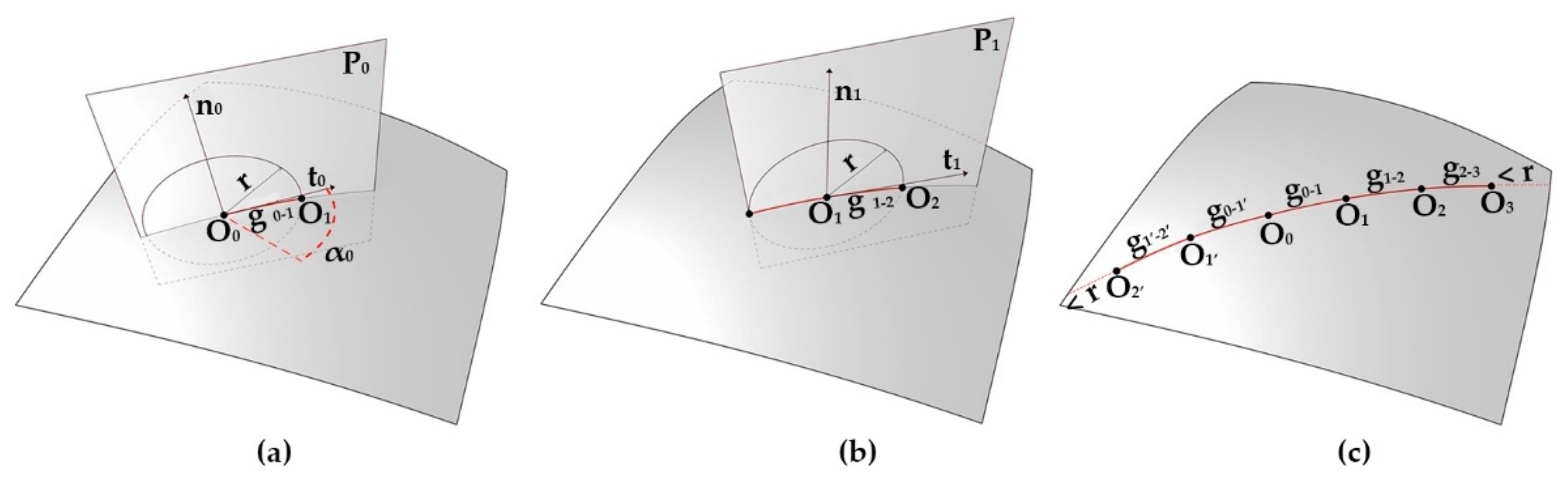
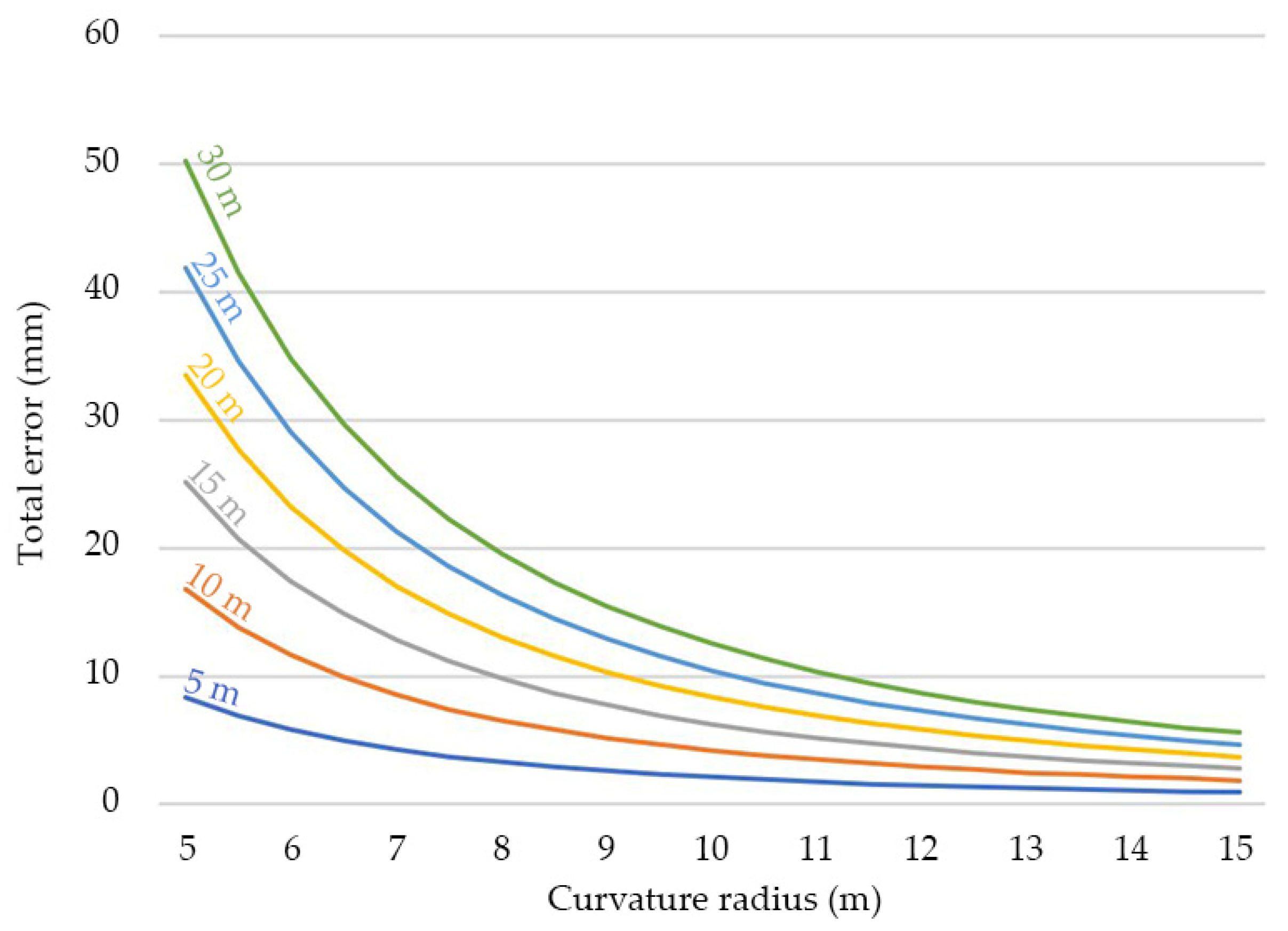
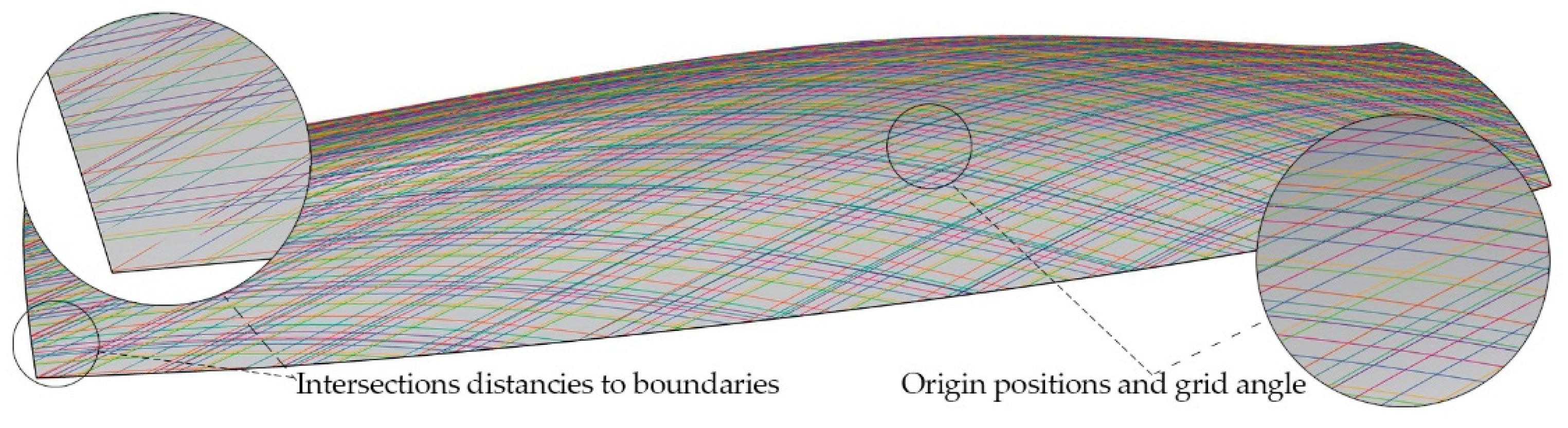
• Starting from O₀, it calculates the intersection between the surface and a circumference with a centre at point O₀, contained in the plane defined by the normal and the tangent vectors with the prescribed direction at O₀. The intersection gives O₁. A geodesic curve g_0-1 is then generated between O₀ and O₁ (Figure 5a). The smaller the circumference radius r, the more accurate the results (algorithm resolution). It should be noted that the plane used is precisely the osculating plane of the plotted geodesic, since it is perpendicular to the tangent plane of the surface.
• The tangent vector of the geodesic g_0-1 is then obtained at point O₁.
• The process is repeated by taking O₁ as the new origin and thus obtaining point O₂. A geodesic curve g_1-2 is then created between O₁ and O₂ (Figure 5b).
• The process is repeated n times until the intersecting circumference does not intersect the surface because the distance from the last origin point to the boundary is smaller than the radius r, breaking the algorithm (Figure 5c).

Figure 6 shows a test of the algorithm with two pairs of geodesic master curves on a test study surface, generated from a pair of orthogonally intersecting parabolic curves in space and a closed base curve. The geodesic curves are generated by applying the procedure described above and varying the starting angle from the same starting point O₀.

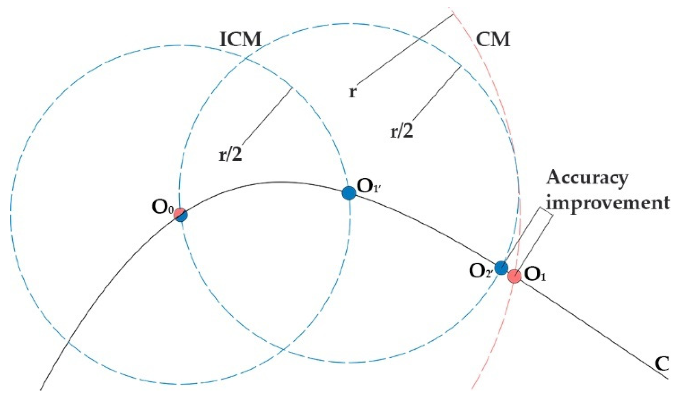
3.1.3. Compass Method Overview

The Compass Method (CM), also known as Tchebyshev net [2,19], is a well-described method for surface meshing in Parametrized Surface Theory [33], corresponding to a mesh over a parametrized surface S: U ⊂ ℝ² → ℝ³, whose directional derivatives (S_u and S_v) over the surface coordinate field satisfy the requirement that the partial derivatives of one parameter have a constant length along the parameter lines of the other parameter:

$${\left|S_{\mathrm{u}}\right|}_{\mathrm{v}}={\left|S_{\mathrm{v}}\right|}_{\mathrm{u}}$$

(5)

The CM has a geometrical approach, shown in Figure 7, where the surface meshing is the result of the intersection of an array of spheres with a given radius all over a surface. Starting from a pair of intersecting curves on the surface, the curves are subdivided by placing spheres with the given radius and using the last intersection obtained recursively as the centre point (Figure 7a). The resulting intersection points on each curve serve as centre points for a tuple of iterating spheres whose intersections with their own and with the surface generate a new array of centre points for the subsequent iterations (Figure 7b). Finally, once the boundary is reached, a two-dimensional net of points is obtained, which can be used as constitutive points for a network of two-dimensional interpolated curves over the surface (Figure 7c).

It is a known problem that meshing surfaces with high local curvature lead to accuracy errors when applying the CM. As mentioned above, the CM computes each point on the mesh by intersecting spheres with the base surface. The desired length for the subdivision over the surface would be the radius of the spheres. To illustrate this problem, Figure 8 shows the analogous issue in planar geometry. For the sake of simplicity, given a circular curve C and a starting point O₀ on the curve, a circumference with radius r can be traced giving the intersection point O₁ on C. The distance between O₀ and O₁ is r and corresponds to the chord of the segment of C between O₀ and O₁. At the same time, finding the endpoint O_1′ of a segment of C with length r starting from O₀, it is observed that O₁ and O_1′ are not coincident, and the distance between them corresponds to the CM error, which depends on the average curvature of each segment of C. Only if C were a straight line would O₁ and O_1′ coincide.

For the circular curve C with radius R in Figure 8, the error due to its curvature can be easily calculated as the difference between the arch length of C for the angle α between O₀ and O₁, and the arch length of C between O₀ and O_1′ (segment of C with length r), which has the same length as the chord of C for the same opening angle α:

$${\mathrm{Arch} \mathrm{length}}_{O_0-O_1}=R \alpha ,$$

(6)

$${\mathrm{Arch} \mathrm{length}}_{O_0-O_1^{\prime }}{=\mathrm{Chord}}_{\alpha }=2R\sin (\alpha /2),$$

(7)

$${\mathrm{Error}}_{\alpha }={\mathrm{Arch} \mathrm{length}}_{\alpha }-{ \mathrm{Chord}}_{\alpha }$$

(8)

The potential impact of this error from applying the CM on a gridshell depends on the length of the laths, the intended mesh subdivision distance, and surface extent, but mainly on the average curvature between each pair of consecutive points.

Figure 9 shows the total deviation in millimetres for five different curve lengths, varying the curvature radius between 5 m and 15 m and considering a usual subdivision radius of 1 m. It is observed that for a 30 m long lath with 5 m radius of curvature, a total error of 50.3 mm is obtained due to the accumulative effect of the described CM accuracy error. The total error decreases exponentially as the radius of curvature increases.

To overcome this drawback, the Improved Compass Method (ICM) was developed [20]. It mitigates such accuracy error through the following procedure: having defined the desired grid node distance r and a resolution factor S, the algorithm runs the CM using a subdistance r/S and dismissing the intermediate S–1 subdivision points before generating the mesh curves. Again, to illustrate the method in Figure 10, the ICM is applied on a planar curve and compared with the CM to show the improvement in accuracy.

Given a curve C and a starting point O₀, applying a CM single step with a desired subdivision distance r, the point O₁ over the curve is obtained. To apply the ICM over C with a subdivision distance r, first, the resolution factor S must be defined, in this case, 2. Given S = 2, ICM uses r/2 as the radius for the intersecting circles and has to perform 2 steps to obtain the subdivision point analogous to the CM subdivision point O₁. The first circle with a centre at O₀ and radius r/2 gets the intersection point O_1′ over C. The second step uses O_1′ as the centre for the second intersecting circle with the same radius r/2, obtaining O_2′ over C. Finally, the ICM removes S–1 intermediate subdivision points, in this case, 1 intermediate subdivision point (O_1′), keeping O_2′ as the final point. The distance between the CM’s O₁ and the ICM’s O_2′ would be the accuracy improvement achieved. The higher the resolution factor S, the greater the improvement in accuracy.

The ICM is more accurate the higher the S. It is perfectly suitable for a single meshing process but has an important drawback when performing an optimisation problem, as it requires much more memory to compute the temporary intersection points over a surface, which slows down the algorithm drastically.

The additional temporary intersection points necessary to obtain a quad mesh can be calculated according to:

$$\mathrm{Aditional} \mathrm{intersections}={\left(S+1\right)}^2- \mathrm{number} \mathrm{of} \mathrm{steps}$$

(9)

The performance of both methods is analysed on the test surface. The CM and the ICM are configured with the same radius, and the latter with S = 3.

According to the results shown in Figure 11, the ICM needs to compute 15 new points to obtain the rest of the three vertices of a new quad mesh (O_0-3), 12 more than the CM. These points are temporal or instrumental intersections. For a single mesh, this difference would have no practical impact, but for an optimisation problem with a few hundred runs, if not thousands, it is a key performance issue to consider.

To overcome this drawback, the authors have developed the Adaptative Compass Method (ACM).

3.1.4. Adaptative Compass Method Proposal

The ACM is conceived to find a balance between accuracy and processing speed. As described above, accuracy problems arise on surfaces with high local curvatures, so this method allows subdividing the surface into n domains with a similar curvature range and adapting the meshing radius to the curvature of each domain.

For each domain, a resolution factor S_n is set with a value from n to 1, where n corresponds to the highest curvature and 1 to the lowest. The mesh radius used in each domain is r/S_n, with r the predefined distance between nodes of the quadrangular mesh. Thus, the larger the S_n, the smaller the mesh radius and, consequently, the denser and more accurate the meshing.

Figure 12 shows the process on the test surface divided into three curvature domains. This starts with the subdivision of the master curves. In this case, for the domain of higher curvature, the master curves are subdivided with r/3; for the area of medium curvature with r/2; and for the area of lower curvature, the standard r is kept (Figure 12a). Once the variable subdivision of the master curves is done, the algorithm runs a CM on the whole surface, adapting the radius of the spheres to the corresponding domain (Figure 12b).

To analyse the improvement in accuracy of the ACM and the ICM over the CM, the distance of the resulting mesh points is measured at two positions on the test surface calculated with the three methods. As already mentioned, the accuracy depends on the curvature of the surface and the extent of the surface covered in each direction, since the meshing error is cumulative in the CM and in its derivative methods (ICM and ACM). The runtime difference between the methods is also compared because of its key importance to the optimisation processes.

Figure 13 shows the test surface and the test points O₁ and O₃. O₁ corresponds to the last subdivision of one of the master curves starting at O₀, which is the longest curve over the surface. O₃ is one of the points on the grid furthest away from the starting point O₀ and from the two master curves. It is obtained after the subdivision process of the master curves (O₀–O₂ and O₀–O_2’) and the meshing over the surface.

The results of the comparison are presented in

Table 1. Comparison of accuracy improvement and runtime of the Improved Compass Method (ICM) and the Adaptative Compass Method (ACM) over the Compass Method (CM).

	Accuracy Improvement (mm)		Multiplier of Runtime
Method	Test Point O1 rρ,mean 1 = 205.71 m Path Length = 15.33 m	Test Point O3 rρ,mean 1 = 17.89 m Path Length = 17.22 m
ICM	4.48	8.46	×6.77
ACM	4.47	8.42	×2.66

¹ Mean curvature radius along the path to reach the specified point.

. With CM being the reference method, both ICM and ACM perform a similar accuracy improvement whatever the mean curvature radius along the path (r_ρ,mean). It is observed that the improvement is greater when computing the subdivision in a ℝ² space (test point O₃) than in a ℝ¹ space (test point O₁). In terms of runtime, the ACM performs 2.54 times faster than the ICM.

3.1.5. Surface Extension and Trimming

As seen before, the laths of the grid are curves interpolated from the points obtained from the ACM. To make the laths reach the surface boundaries, it is necessary for the ACM to continue beyond those boundaries for at least one iteration over the extended surface, so the last points for the interpolation are outside the boundaries allowing the interpolated curves to intersect with them. Therefore, it is necessary to implement an intermediate step in the process before generating the laths from the grid of points: the surface must be extended as necessary, with continuity of tangency and curvature, to get points outside the surface and make the laths intersect the perimeter [34].

In Figure 14, the ACM is performed over an extended version of the surface. The mesh is then generated by interpolating the curves at these points (Figure 14a). The points are removed, and the laths are trimmed at the surface boundary (Figure 14b). This extension process may be large when dealing with surfaces with noticeably uneven length and width dimensions to avoid unreachable blind zones for the spheres to intersect.

3.2. Stress Evaluation

Once the grid curves are obtained (lath axes), the algorithm evaluates the bending moments along the laths by applying beam theory and the concepts of curve and surface geometry.

As is known, the moment value M that is produced in a cross-section due to curvature can be obtained from:

$$M=k E I,$$

(10)

where k is the modulus of the curvature vector at that cross-section, E is the Young’s modulus of the material, and I is the second moment of the cross-section area with respect to the bending axis.

The maximum bending stress at the cross-section occurs at the outer fibres and can be obtained by using:

$${\sigma }_{\mathrm{m}}=k E \frac{h}{2},$$

(11)

where h denotes the cross-section depth in the bending plane.

Since the laths of a gridshell are usually bent with respect to their two main bending axes, it is necessary to know the curvature values associated with each of these axes.

If it is accepted that the faces of the laths are tangent and normal to the design gridshell surface, then the curvatures of the laths with respect to the two main bending axes coincide with the normal and geodesic curvatures of the lath directrix, k_N and k_G, respectively. As seen in Section 3.1.1 (Equations (3) and (4)) the values of k_N and k_G can be easily calculated at any point on the curve from the curvature vector $\overrightarrow{k}$ of the curve and the angle formed between it and the vector $\overrightarrow{N}$ normal to the surface.

Denoting the y-axis and the z-axis as the bending axes of the lath cross-section, tangent and perpendicular to the surface of the gridshell respectively, and b and h as the cross-sectional dimensions associated with each axis, the corresponding bending moments and the maximum initial bending stresses in a given cross-section due to the existence of k_N and k_G curvatures can be calculated from Equations (12)–(15), where σ_m,y is the maximum initial bending stress due to normal curvature k_N and σ_m,z is the maximum initial bending stress due to geodesic curvature k_G,

$$M_{\mathrm{y}}=k_{\mathrm{N}} E I_{\mathrm{y}},$$

(12)

$${\sigma }_{\mathrm{m},\mathrm{y}}=k_{\mathrm{N}} E \frac{h}{2},$$

(13)

$$M_{\mathrm{z}}=k_{\mathrm{G}} E I_{\mathrm{z}},$$

(14)

$${\sigma }_{\mathrm{m},\mathrm{z}}=k_{\mathrm{G}} E \frac{b}{2}$$

(15)

The maximum initial bending stress σ_m,total in a cross-section subjected to two curvatures can be obtained from the sum of the maximum initial bending stresses due to each curvature, according to:

$${\sigma }_{\mathrm{m},\mathrm{total}}=\frac{E}{2}\left(k_{\mathrm{N}} h+k_{\mathrm{G}} b\right)$$

(16)

The developed algorithm calculates the $\overrightarrow{k}$ and $\overrightarrow{N}$ vectors along the curves on the grid and computes M_y, M_z, σ_m,y, σ_m,z, and σ_m,total for the user-defined values of E, b, and h.

Figure 15 shows the visualisation of the results provided by the algorithm on the test surface for a grid of Eucalyptus globulus laths (E = 18,108 MPa) [7] of 50 mm width and 25 mm depth.

3.3. Design Constraints

The design constraints are the target surface and the study area. In this work, the PEMADE gridshell is used to verify the proposed design process. It is an innovative 24 m long elastic timber gridshell recently developed by the authors, with a double curved surface and a strong difference between its length and width. The gridshell is supported only on its short sides by two transverse glulam arches generating two 4.5 m cantilevers (Figure 1).

The area of the gridshell with the highest bending stresses due to external loads is the area close to the supports and is therefore established as the study area in which to minimise the initial bending stresses. Figure 16 shows the geometric definition of the target surface of the PEMADE gridshell and the study area.

4. Optimisation Method

4.1. Design Variables

As described in previous sections, genes are the design variables that, combined using the algorithm with a certain value, conform to the individual’s chromosomes or solution vectors. Figure 17 shows the four genes used by the algorithm, two of which define the topological variants of each solution, while the other two define the size variants of the solution.

The moving area of topological gene 1 (origin position) is defined as the portion of surface enclosed by the polygon resulting from joining certain points over the bisectors of the geodesic master curves. These points lie at the midpoint of the segment between starting point O₀ and the adjacent intersections in the bisector directions. The surface of the PEMADE gridshell is symmetric. In this special case, the moving area is defined as a curve (corresponding to the intersection curve between the plane of symmetry and the surface) that coincides with bisector 1 (curve G3 in Figure 16), with a length limited to half the length between two adjacent nodes on that intersection curve. It is computed as parameter t over the moving curve from 0.00 to 1.00.

Topological gene 2 (grid angle) is defined as a range of admissible angles between the geodesic master curves. In the PEMADE gridshell, 0.30 and 1.50 radians.

Both gene 1 and gene 2 are continuous variables, a floating number with two decimal places.

Size genes 3 and 4 are the width and depth of the cross-section. The size genes are discrete, with predefined allowable values varying in 5 mm steps within a range for each gene. Gene 3 (cross-section depth) varies between 25 mm and 50 mm, while gene 4 (cross-section width) ranges between 50 mm and 80 mm. This range covers the cross-section sizes used in the most popular elastic timber gridshells.

4.2. Optimiser and Fitness Function

In this work, the Strong Pareto Evolutionary Algorithm (SPEA-2) is used, which outperforms other GA algorithms [35] and has the unique feature of storing in a parallel file the outperforming solutions, which can be examined by the DM for the selection of the final solution along with the total population.

Although SPEA-2 is conceived to solve multi-objective optimization problems where the solution is a field of non-dominated vector solutions known as Pareto optima set, the design process presented in this work sets up the problem as a single objective where the optimal solution is a single vector [36], the strictly minimal solution regarding the fitness function after all generations, while keeping all provided solutions available for further analysis. The intention of this decision is to give the DM the opportunity to analyse the entire solution space, where near-optimal solutions that meet additional requirements can be found.

Once the parametric model is built, the SPEA-2 can be set up. It is necessary to establish the single-objective fitness function (FF), which is the minimisation of the initial bending stress in the study area. The design vector is given as:

$$d=\left\{g_1,\dots ,g_n\right\},$$

(17)

where n = 4 and g_n are the genes described in Section 4.1.

With the dominant σ_m,total,dom being the highest value at any point O of the study area, obtained from Equation (16), the FF can be formally stated as:

$$\min f(d)=\min {({\sigma }_{\mathrm{m},\mathrm{total},\mathrm{dom}})}_O$$

(18)

Finally, the population of each generation and the number of total generations must be defined. This should be done by trial and error to fine-tune the settings for each specific problem. For the PEMADE gridshell, the number of individuals for Step 1 was set to 100 and the maximum number of generations to 10. For Step 2, 20 individuals and 10 generations were established.

5. Decision Making

Once the SPEA-2 algorithm completes the last generation or converges to a solution state where no improvement is achieved, it stops and provides both the history of individual solutions generated and the Elite solutions found in each generation. It is time for the DM to analyse the solution space and search among them for the final selected solution.

There is at least one solution for each cross-section size considered, which ensures that the initial bending stress is minimal in the study area. In addition to these, there may be other valid solutions to the design problem that, being near-minimal, improve other aspects not considered by the FF.

In a real design process, the final solution to be adopted depends not only on mechanical criteria such as the maximum initial bending stress, but also on other factors such as the available cross-sections, the minimum cross-section width to be used (which is usually determined by the diameter of the fastener), the minimum end distances to the fasteners, or non-programmed criteria, such as aesthetic criteria. In addition, during the design process, it may be required to change the size of the initially chosen cross-section for reasons beyond the DM’s control. Therefore, it is necessary to work with a space of valid solutions rather than a single optimal solution found by the FF.

The process proposed in this work consists of searching for a near-optimal solution within the solution space offered by SPEA-2 by means of additional specific constraints incorporated by the DM, in a two-step process:

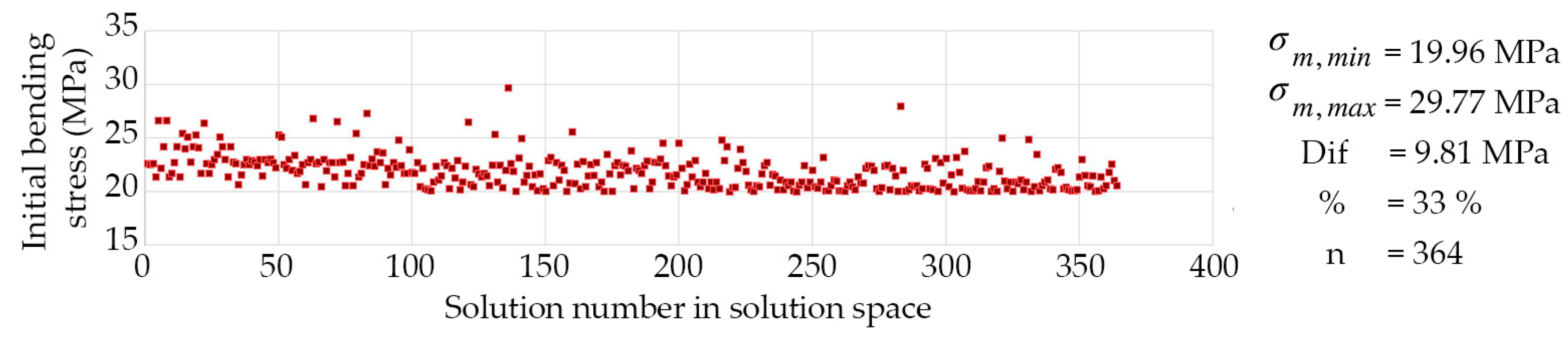
• In Step 1, the field of solutions is limited by incorporating the maximum initial bending stress that cannot be exceeded in the study area. This value must be lower than the design strength of the material, maintaining the structural reserve necessary to resist external loads, and considering the rheological phenomena of the material and the multilayer system action [37]. In this research, Eucalyptus globulus laths GL45 [7,38] and a maximum initial bending stress of 33 MPa were considered. This constraint provides a set of valid cross-section sizes for the DM to choose from.
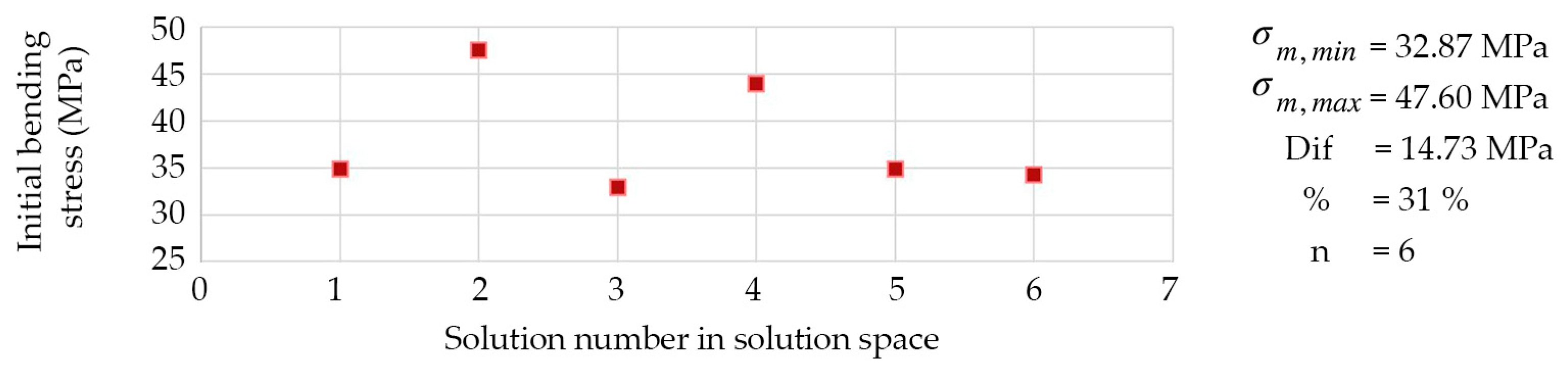
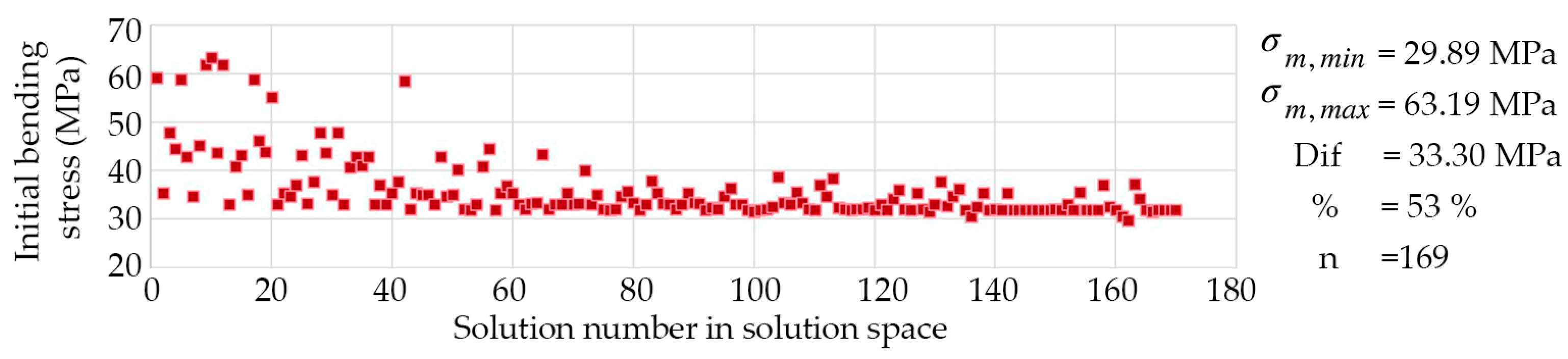
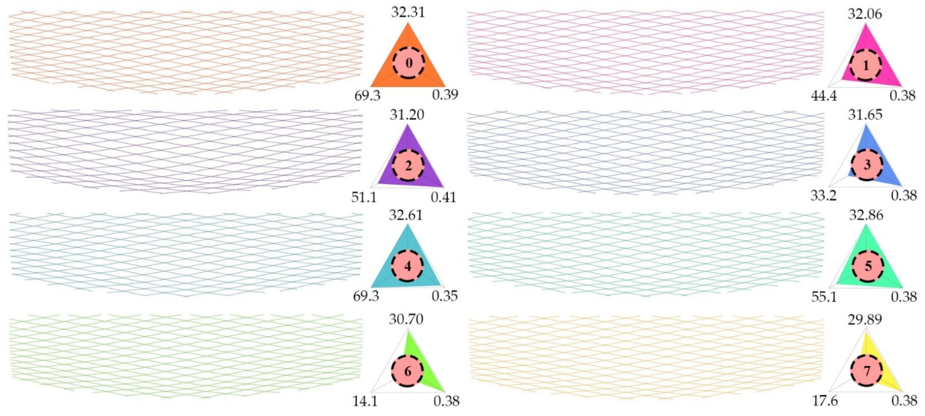
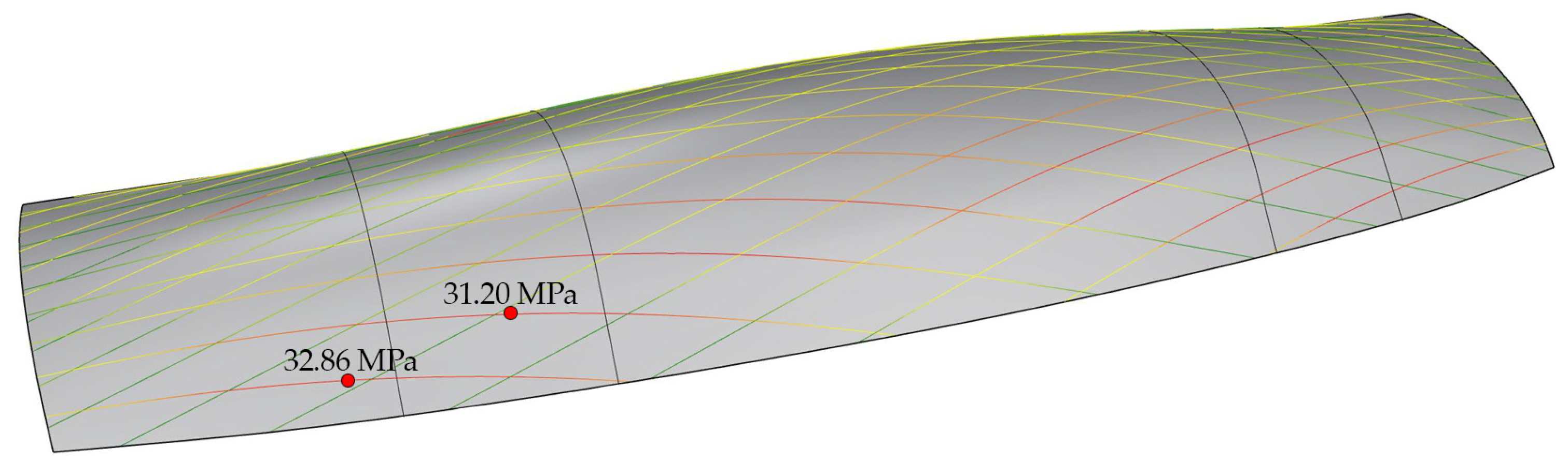
• In Step 2, once the cross-section size is chosen by the DM, a new optimisation process is run in which the algorithm offers a field of near-optimal solutions for the DM to choose according to other non-programmed issues, such as end distances or aesthetic aspects. Step 2 deals only with the topologic genes once the size genes become fixed.

6. Results and Discussion

The parametric model generates meshes at the instance of the optimisation algorithm over the PEMADE surface and simulates the initial bending stress by applying the process described in the previous sections, considering E = 18,108 MPa [7].

Figure 18 shows the six-step algorithm process for an individual with gene values of 0.072 origin position, 0.4 radians grid angle, 40 mm depth, and 70 mm width. For each individual, the parametric model sends the results (mesh and initial stresses) and its gene values to the optimisation algorithm for evaluation.

In Step 1, the optimisation algorithm produces a solution space of 1091 individuals (100 individuals in 10 generations plus 91 non-dominated solutions) whose maximum initial bending stresses in the surface study area range from 19.96 MPa to 88.78 MPa depending on the cross-section size.

Table 2. Step 1 optimisation outcome.

Depth (mm)		Width (mm)
		50	55	60	65	70	75	80
25	σm,min (MPa)	19.96	21.54	23.19	27.85	30.69	31.92	31.70
	σm,max (MPa)	29.77	48.82	43.07	51.27	44.87	43.52	36.98
	AI 1 (MPa)	9.81	27.28	19.88	23.42	14.18	11.6	5.28
	RI 2	0.33	0.56	0.46	0.46	0.32	0.27	0.14
	n	364	75	15	4	7	8	6
30	σm,min (MPa)	21.00	22.53	24.30	29.24	31.37	32.88	31.49
	σm,max (MPa)	44.38	51.86	44.94	56.17	59.74	47.60	60.00
	AI 1 (MPa)	23.38	29.33	20.64	26.93	28.37	14.72	28.51
	RI 2	0.53	0.57	0.46	0.48	0.47	0.31	0.48
	n	184	86	22	12	10	6	11
35	σm,min (MPa)	22.39	23.92	25.41	29.80	29.08 1	31.23 1	33.90
	σm,max (MPa)	44.97	60.51	64.53	51.30	60.27	64.54	54.67
	AI 1 (MPa)	22.58	36.59	39.12	21.5	30.29	33.31	20.77
	RI 2	0.50	0.60	0.61	0.42	0.50	0.52	0.38
	n	16	34	14	18	13	10	2
40	σm,min (MPa)	25.31	26.56	27.80	29.40	31.02	32.20	55.92
	σm,max (MPa)	63.66	59.00	55.25	74.41	57.35	68.15	70.20
	AI 1 (MPa)	38.35	32.44	27.45	45.01	26.33	35.95	14.28
	RI 2	0.60	0.55	0.50	0.60	0.46	0.53	0.20
	n	7	23	10	10	6	19	2
45	σm,min (MPa)	30.11	29.18	31.58	36.14	35.24	34.95	38.07
	σm,max (MPa)	53.43	70.54	72.22	81.91	77.71	66.66	78.66
	AI 1 (MPa)	23.32	41.36	40.64	45.77	42.47	31.71	40.59
	RI2	0.44	0.59	0.56	0.56	0.55	0.48	0.52
	n	6	19	13	6	12	7	11
50	σm,min (MPa)	33.52	32.24	52.27	61.59	49.61	47.31	41.69
	σm,max (MPa)	44.51	75.87	52.27	88.78	49.61	81.84	41.69
	AI 1 (MPa)	10.99	43.63	0	27.19	0	34.53	0
	RI2	0.25	0.58	0	0.31	0	0.42	0
	n	5	7	1	3	1	5	1

¹ Absolute improvement, AI = σ_m,max − σ_m,min; ² Relative improvement, RI = 1 − σ_m,max/σ_m,min.

shows the main results for all the cross-sections generated according to the defined range of size genes. For each of the cross-sections, the minimum and maximum values (σ_m,min and σ_m,max) of the maximum initial bending stress in the study area, the absolute improvement (AI = σ_m,max − σ_m,min) and the relative improvement (RI = 1 − σ_m,max/σ_m,min) obtained during the optimisation process, as well as the number of individuals generated (n) are presented.

As expected, the minimum value (19.96 MPa) is obtained for the smallest cross-section (50 × 25 mm²), where the algorithm focuses its search generating a total of 364 individuals. The absolute improvement achieved in this cross-section is 9.81 MPa and the relative improvement is 33%.

Figure 19 shows the value of the maximum initial bending stress in the study area for the 364 solution individuals with 50 × 25 mm² cross-section. The evolutionary optimisation process considerably increases the number of individuals with maximum stress values close to the minimum (around 20 MPa) which offers a wide space of possible solutions for the DM.

In the rest of cross-sections, the optimisation algorithm generates a much smaller number of individuals—generally smaller the larger the cross-section—even a single individual in some of the larger cross-sections. This is due to the internal functioning of the optimisation algorithm. Those solutions far from the fittest at the time of processing a generation, are more likely prevented from passing their genes to the next generation; thus, this area of the solution vector escape is skipped by the algorithm, and no further search is performed in this area throughout the rest of the optimisation. Although the algorithm does not perform an exhaustive search in these cross-sections, the results obtained give an idea of the maximum stress and improvement values that can be achieved.

The results show absolute improvements between 5.28 MPa and 45.01 MPa and relative improvements between 14% and 61%, highlighting the great importance of the optimisation process. Furthermore, it should not be forgotten that in an optimisation process focused on a single cross-section, the minimum stress values presented in Table 2 should foreseeably be reduced, and consequently, the improvements should increase.

The results obtained in Step 1 allow the DM to have an overview of the cross-sections that can be used for a given maximum value of initial bending stress. For example, for a value of 15 MPa, no cross-section is available, so it would be necessary to change the material or the shape of the surface. For a value of 20 MPa, the only a priori valid cross-section is 50 × 25 mm², although it may be interesting to carry out a more exhaustive search through a new optimisation process focused on other cross-sections whose σ_m,min slightly exceeds this value, such as 50 × 30 mm² or 55 × 25 mm², in which some individual that meets this condition could perhaps be found.

In this work, the maximum value for initial bending stress was set at 33 MPa. The staggered dashed line in Table 2 separates the cross-sections that meet this condition. The DM can choose from any of the cross-sections in the group or look at some of the nearby cross-sections that are left out, if necessary. In the case presented here, the 75 × 30 mm² cross-section was chosen as a result of the minimum width imposed by the selected bolt diameter (12 mm) and the maximum timber utilisation that could be achieved from the cross-sections available in the sawmill. As can be seen in Table 2, the optimisation algorithm in Step 1 only provided six individuals for the chosen cross-section, of which only 1 had a stress below 33 MPa (Figure 20), so a broader search was necessary.

In Step 2, a second optimisation process was carried out focusing on the chosen 75 × 30 mm² cross-section. Figure 21 shows the evolution of the maximum initial bending stresses for this case. The optimiser was programmed to create 200 individuals in 10 generations and stopped at 169 individuals as no improvement was achieved. The optimal solution yielded a maximum initial bending stress of 29.89 MPa in this step, 9% lower than the 32.88 MPa reached in Step 1.

The solution space offers 63 individuals with a maximum stress below 33 MPa, of which only 8 individuals are singular. This is because, as the search space narrows towards an optimal, the range for the gene configurations becomes smaller, and some repetitions occur since the number of individuals per generation is fixed regardless of the size of the search space. These 8 solutions constitute the ultimate design space for the DM.

Figure 22 shows the grid corresponding to the selected solutions, including the values of maximum stress and the topological genes. At first glance, the differences between these solutions may seem subtle, but there are considerable differences in the intersections of the laths in the areas close to the short edges of the boundary. This is of great importance from a structural point of view since, in structural timber design, a minimum distance from the connection to the ends of the laths must be complied with. Solutions in which the intersections are too close to the short edges of the boundary (solutions 0, 4 and 5) are discarded because they require special solutions for the joints. Solutions with intersections too far away from the short edges (solutions 1, 3, 6 and 7) are not chosen for aesthetic reasons.

In Figure 23, the 8 solutions are superimposed to compare the designs and to get an idea of the differences between them. Considering these additional design constraints, the final solution selected was grid number 2, shown in Figure 24, which operates with a maximum initial bending stress of 31.2 MPa in the study area, an opening angle of 0.41 rad, and a relative position of the origin along the allowed moving curve of 51.1%.

7. Gridshell Realisation

The chosen grid solution was used for the construction of the PEMADE gridshell designed by the authors, a permanent roof structure to cover the new timber warehouse of the Timber Engineering Laboratory (PEMADE) of the University of Santiago de Compostela in Lugo, Spain. The structure is supported exclusively by two separate arches of Pinus radiata glulam resting on steel supports (Figure 1). This design allowed for large cantilevers at the ends to protect the stored material from lateral rainfall.

The grid geometry was used as the basis for the development of the structural analysis model, with which the performance of the chosen geometric solution and cross-section were analysed and validated. Information on this model can be found in previous works by the authors [9,31]. The grid geometry was also applied as the basis for the development of a 3D model of the structure (Figure 25) used for the definition of the construction and execution details. A 3D model of the formwork used for the construction of the gridshell made it possible to obtain the points where the laths pass through.

The execution of the exact grid geometry was ensured using temporary timber pieces placed on the formwork, which allowed the precise placement of the laths on each of the arches. Figure 26 shows a general view of the formwork during the placement of the first family of laths (Figure 26a) and a detail of the temporary timber pieces for their placement (Figure 26b).

Figure 27 shows a detail of the final appearance of the short edge of the structure, where the distance from the last connection to the end of the laths was the crucial aspect in the DM’s decision process for the choice of the final grid.

8. Conclusions

This work provides a complete computational workflow for the design process of elastic timber gridshells with quadrangular meshing in order to choose the grid topology and cross-section size in the usual case where the target surface is imposed. This includes the development of a parametric model for the surface meshing and the evaluation of the initial bending stresses, as well as a genetic optimisation algorithm.

A geometric method for mesh generation is developed, called in this work the Adaptative Compass Method. The method adapts the accuracy of the mesh to the local curvature of the surface, achieving similar accuracies to other existing methods but with a substantial reduction in computational time. This improvement is of great interest in optimisation processes where it is necessary to generate hundreds or thousands of meshes.

The results show that the optimisation process succeeds in significantly reducing the initial bending stresses and offers an interesting design space for the Decision Maker. This space consists of a set of near-optimal solutions with sufficiently diverse geometries from which the final solution can be chosen according to additional non-programmed requirements, such as constructional or aesthetic ones.

The proposed design process has been validated and successfully implemented in the design of a permanent elastic timber gridshell.

Further research extending the design framework to quadrangular meshes with a non-constant distance between nodes (e.g., pseudo-geodesic patterns) and multi-objective searches would be of interest.

References

1. Dyvik, S.H.; Manum, B.; Rønnquist, A. Gridshells in Recent Research—A Systematic Mapping Study. Appl. Sci. 2021, 11, 11731. [Google Scholar] [CrossRef]
2. Hennicke, J.; Matsushita, K.; Otto, F.; Sataka, K.; Schaur, E.; Shirayanagi, T.; Gröbber, G. IL 10 Gitterschalen; Institut für Leichte Flächentragwerke (IL): Stuttgart, Germany, 1974. [Google Scholar]
3. Lefevre, B.; Douthe, C.; Baverel, O. Buckling of elastic gridshells. J. Int. Assoc. Shell Spat. Struct. 2015, 56, 153–171. [Google Scholar]
4. Collins, M.; Cosgrove, T. Dynamic relaxation modelling of braced bending active gridshells with rectangular sections. Eng. Struct. 2019, 187, 16–24. [Google Scholar] [CrossRef]
5. Quinn, G.C.; Gengnagel, C.; Williams, C.J.K. Comparison of erection methods for long-span strained grid shells. In Proceedings of the International Association for Shell and Spatial Structures (IASS) Symposium, Amsterdam, The Netherlands, 17–20 August 2015. [Google Scholar]
6. Ghiyasinasab, M.; Lehoux, N.; Ménard, S. Production Phases and Market for Timber Gridshell Structures: A State-of-the-Art Review. BioResources 2017, 12, 9538–9555. [Google Scholar] [CrossRef]
7. Lara-Bocanegra, A.J.; Majano-Majano, A.; Arriaga, F.; Guaita, M. Eucalyptus globulus finger jointed solid timber and glued laminated timber with superior mechanical properties: Characterisation and application in strained gridshells. Constr. Build. Mater. 2020, 265, 120355. [Google Scholar] [CrossRef]
8. Lara-Bocanegra, A.J.; Majano-Majano, A.; Arriaga, F.; Guaita, M. Long-term bending stress relaxation in timber laths for the structural design of lattice shells. Constr. Build. Mater. 2018, 193, 565–575. [Google Scholar] [CrossRef]
9. Lara-Bocanegra, A.J.; Majano-Majano, A.; Ortiz, J.; Guaita, M. Structural Analysis and Form-Finding of Triaxial Elastic Timber Gridshells Considering Interlayer Slips: Numerical Modelling and Full-Scale Test. Appl. Sci. 2022, 12, 5335. [Google Scholar] [CrossRef]
10. Douthe, C.; Caron, J.F.; Baverel, O. Gridshell structures in glass fibre reinforced polymers. Constr. Build. Mater. 2010, 24, 1580–1589. [Google Scholar] [CrossRef]
11. Natterer, J.; Burger, N.; Müller, A.; Natterer, J. Holzrippendächer in Brettstapelbauweise—Raumerlebnis durch filigrane Tragwerke. Bautechnik 2000, 77, 783–792. [Google Scholar] [CrossRef]
12. Adriaenssens, S.; Barnes, M.; Harris, R.; Williams, C. Dynamic relaxation: Design of a strained timber gridshell. In Shell Structures for Architecture: Form Finding and Optimization; Adriaenssens, S., Block, P., Veenendaal, D., Williams, C., Eds.; Routledge: Abingdon, UK, 2014; pp. 89–102. [Google Scholar]
13. Douthe, C.; Baverel, O.; Caron, J.-F. Form-finding of a grid shell in composite materials. J. Int. Assoc. Shell Spat. Struct. 2006, 47, 53–62. [Google Scholar]
14. Lafuente Hernández, E.; Baverel, O.; Gengnagel, C. On the Design and Construction of Elastic Gridshells with Irregular Meshes. Int. J. Space Struct. 2013, 28, 161–174. [Google Scholar] [CrossRef]
15. D’Amico, B.; Kermani, A.; Zhang, H. Form finding and structural analysis of actively bent timber grid shells. Eng. Struct. 2014, 81, 195–207. [Google Scholar] [CrossRef]
16. Bouhaya, L.; Baverel, O.; Caron, J.-F. Mapping two-way continuous elastic grid on an imposed surface. In Proceedings of the International Association for Shell and Spatial Structures (IASS) Symposium, Valencia, Spain, 28 September–2 October 2009. [Google Scholar]
17. D’Amico, B.; Kermani, A.; Zhang, H. A form finding method for post formed timber grid shell structures. In Proceedings of the World Conference on Timber Engineering, Quebec City, QC, Canada, 10–14 August 2014. [Google Scholar]
18. Harris, R.; Haskins, S.; Roynon, J. The Savill Garden gridshell: Design and construction. Struct. Eng. 2008, 86, 27–34. [Google Scholar]
19. Baverel, O.; Caron, J.-F.; Tayeb, F.; Du Peloux, L. Gridshell in Composite Materials: Construction of a 300 m2 Forum for the Solidays’ Festival in Paris. Struct. Eng. Int. 2012, 3, 408–414. [Google Scholar] [CrossRef] [Green Version]
20. Popov, E.V. Geometric Approach to Chebyshev Net Generation Along an Arbitrary Surface Represented by NURBS. In Proceedings of the International Conference Graphicon, Nizhny Novgorod, Russia, 29 April 2002. [Google Scholar]
21. Deb, K. Multi-objective Genetic Algorithms: Problem Difficulties and Construction of Test Problems. Evol. Comput. 1999, 7, 205–230. [Google Scholar] [CrossRef]
22. Jakiela, M.J.; Chapman, C.; Duda, J.; Adewuya, A.; Saitou, K. Continuum structural topology design with genetic algorithms. Comput. Methods Appl. Mech. Eng. 2000, 186, 339–356. [Google Scholar] [CrossRef]
23. Holland, J.H. Adaptation in Natural and Artificial Systems. An Introductory Analysis with Applications to Biology, Control, and Artificial Intelligence; MIT Press Ltd.: Cambridge, MA, USA, 1992. [Google Scholar]
24. Rocha, M.; Neves, J.M. Preventing Premature Convergence to Local Optima in Genetic Algorithms via Random Offspring Generation. In Multiple Approaches to Intelligent Systems; Springer: Berlin, Germany, 1999. [Google Scholar]
25. Konak, A.; Coit, D.W.; Smith, A.E. Multi-objective optimization using genetic algorithms: A tutorial. Reliab. Eng. Syst. Saf. 2006, 91, 992–1007. [Google Scholar] [CrossRef]
26. Deb, K.; Pratap, A.; Agarwal, S.; Meyarivan, T. A fast and elitist multiobjective genetic algorithm: NSGA-II. IEEE Trans. Evol. Comput. 2002, 6, 182–197. [Google Scholar] [CrossRef] [Green Version]
27. Winslow, P.; Pellegrino, S.; Sharma, S.B. Multi-objective optimization of free-form grid structures. Struct. Multidiscip. Optim. 2010, 40, 257–269. [Google Scholar] [CrossRef]
28. Richardson, J.N.; Adriaenssens, S.; Coelho, R.F.; Bouillard, P. Coupled form-finding and grid optimization approach for single layer grid shells. Eng. Struct. 2013, 52, 230–239. [Google Scholar] [CrossRef]
29. Grande, E.; Imbimbo, M.; Tomei, V. Role of global buckling in the optimization process of grid shells: Design strategies. Eng. Struct. 2018, 156, 260–270. [Google Scholar] [CrossRef]
30. Bouhaya, L.; Baverel, O.; Caron, J.-F. Optimization of gridshell bar orientation using a simplified genetic approach. Struct. Multidiscip. Optim. 2014, 50, 839–848. [Google Scholar] [CrossRef] [Green Version]
31. Lara-Bocanegra, A.J.; Roig, A.; Majano-Majano, A.; Guaita, M. Innovative design and construction of a permanent elastic timber gridshell. Proc. Inst. Civ. Eng.—Struct. Build. 2020, 173, 352–362. [Google Scholar] [CrossRef]
32. Schiling, E.; Barthel, R. Suchov’s bent networks: The impact of network curvature on Suchov’s gridshell designs. Structures 2021, 29, 1496–1506. [Google Scholar] [CrossRef]
33. Crane, K.; Wardetzky, M. A glimpse into discrete differential geometry. Not. Am. Math. Soc. 2017, 64, 1153–1159. [Google Scholar] [CrossRef]
34. Du Peloux, L.; Baverel, O.; Caron, J.-F.; Tayeb, F. From shape to shell: A design tool to materialize freeform shapes using gridshells structures. In Proceedings of the Design Modelling Symposium, Berlin, Germany, 28 September–2 October 2013. [Google Scholar]
35. Zitzler, E.; Deb, K.; Thiele, L. Comparison of multiobjective evolutionary algorithms: Empirical results. Evol. Comput. 2000, 8, 173–195. [Google Scholar] [CrossRef] [Green Version]
36. Fonseca, C.M.; Fleming, P.J. Genetic algorithms for multiobjective optimization—Formulation, discussion and generalization. In Proceedings of the fifth International Conference on Genetic Algorithms, Urbana, IL, USA, 17–19 July 1993. [Google Scholar]
37. Lara-Bocanegra, A.J. Elastic timber gridshells. From material to construction. Ph.D. Thesis, Universidad Politécnica de Madrid, Madrid, Spain, 13 June 2022. [Google Scholar]
38. Lara-Bocanegra, A.J.; Majano-Majano, A.; Crespo, J.; Guaita, M. Finger-jointed Eucalyptus globulus with 1C-PUR adhesive for high performance engineered laminated products. Constr. Build. Mater. 2017, 135, 529–537. [Google Scholar] [CrossRef]
Figure 1. Exterior views of PEMADE gridshell.
Applsci 13 00063 g001
Figure 2. Workflow diagram of the proposed design process.
Applsci 13 00063 g002
Figure 3. Frenet trihedron (a) and Darboux trihedron (b).
Applsci 13 00063 g003
Figure 4. Relationship between the Frenet and Darboux trihedrons in space (a) and projected (b).
Applsci 13 00063 g004
Figure 5. Generation of a geodesic curve from a point and a direction vector: (a) First iteration from the origin point; (b) Second iteration from the point resulting from the first iteration; (c) Resulting geodesic curve.
Applsci 13 00063 g005
Figure 6. Geodesic master curves from a starting point and two directions.
Applsci 13 00063 g006
Figure 7. Compass Method: (a) Initial curves subdivision; (b) Surface subdivision process; (c) Resulting mesh.
Applsci 13 00063 g007
Figure 8. Compass Method accuracy error.
Applsci 13 00063 g008
Figure 9. Compass Method error for a 1 m subdivision mesh.
Applsci 13 00063 g009
Figure 10. Improved Compass Method versus Compass Method.
Applsci 13 00063 g010
Figure 11. Compass Method (a) and Improved Compass Method (b) comparison.
Applsci 13 00063 g011
Figure 12. Adaptative Compass Method: (a) Surface curvature domains and subdivision of master curves; (b) Resulting net of points.
Applsci 13 00063 g012
Figure 13. Test surface and curvature radius diagrams of the paths to the test points O1 and O3.
Applsci 13 00063 g013
Figure 14. (a) Extended mesh and laths over the extended surface; (b) Trimmed mesh result over the test surface.
Applsci 13 00063 g014
Figure 15. Evaluation of curvatures and initial bending stresses on a grid over the test surface: (a) Normal curvature and maximum bending stress σm,y; (b) Geodesic curvature and maximum bending stress σm,z; (c) Curvature; (d) Maximum total bending stress σm,total.
Applsci 13 00063 g015
Figure 16. PEMADE gridshell. Geometric definition of the target surface and study area.
Applsci 13 00063 g016
Figure 17. Solution vector composition (chromosome’s genes).
Applsci 13 00063 g017
Figure 18. Parametric model and simulation applied on the PEMADE surface: (a) Extended surface and geodesic master curves; (b) Surface subdivision based on curvature and adaptative subdivision of geodesic curves; (c) Grid points by Adaptative Compass Method; (d) Untrimmed mesh; (e) Trimmed mesh; (f) Initial stresses.
Applsci 13 00063 g018
Figure 19. Evolution of initial bending stress for 50 × 25 mm2 cross-section in Step 1.
Applsci 13 00063 g019
Figure 20. Evolution of initial bending stress for 75 × 30 mm2 cross-section in Step 1.
Applsci 13 00063 g020
Figure 21. Evolution of initial bending stress for 75 × 30 mm2 cross-section in Step 2.
Applsci 13 00063 g021
Figure 22. Space solution for 75 × 30 mm2 cross-section, with maximum initial bending stress of less than 33 MPa in the study area. In the triangles, the middle number is the solution number; the upper vertex provides the maximum initial bending stress in the study area; the lower left vertex is the origin position in % (topological gene 1), and the right vertex is the opening angle in radians (topological gene 2).
Applsci 13 00063 g022
Figure 23. Superimposed selected solutions.
Applsci 13 00063 g023
Figure 24. Final selected solution.
Applsci 13 00063 g024
Figure 25. Selected grid solution and 3D model of the gridshell and formwork.
Applsci 13 00063 g025
Figure 26. Gridshell during construction: (a) Curving process of the first family of laths; (b) Detail of the placement of the laths on the formwork.
Applsci 13 00063 g026
Figure 27. Detail of the end of the laths at the short edge of the structure.
Applsci 13 00063 g027