Different Path Planning Techniques for an Indoor Omni-Wheeled Mobile Robot: Experimental Implementation, Comparison and Optimization

Abstract

Omni-wheeled mobile robots (Omni WMRs) are commonly used in indoor navigation applications like surveillance, search and rescue, and autonomous transportation. They are always characterized by their versatility, mobility and high payload. This paper presents the mechatronic design, low-level control and high-level control of an indoor 4 Omni-Wheeled Mobile Robot (4OWMR). Since autonomy and path planning are research necessities for WMRs, four heuristic and probabilistic path-planning techniques are chosen for experimental implementation. The selected techniques are PRM (Probabilistic Roadmaps), RRT (Rapidly exploring Random Tree), RRTSTAR (RRT*), and ASTAR (A*) algorithms. The proposed environments are static, expressed by maps with unknown nodes and obstacles. Local path planning is implemented with simultaneous localization and mapping (SLAM). Path planning techniques are programmed, and the obtained paths are optimized by a multi-objective genetic algorithm technique to ensure the shortest path and its smoothness. The optimized paths are deployed to the 4OWMR. The obtained results are compared in terms of travel time, travel distance, average velocity and convergence error. A ranking technique is utilized to rank the obtained results and show the most preferred technique in terms of energy consumption and convergence accuracy in addition to the overall ranking. Experimental results showed that the Hybrid A* algorithm produced the best-generated paths with respect to other techniques.

1. Introduction

Mobile robotics has become one of the most expansive points of research nowadays [1]. They are usually used to substitute humans in different life activities, either indoors or outdoors. They are already widely used in inspection tasks, transportation, surveillance, explorations, museum guides, medical services, and entertainment [2].

Generally, mobile robotics is one of the promising technologies in the global market. Recent research in mobile robots is concerned with Autonomous wheeled mobile robots (AWMRs). They are a vehicle that uses onboard sensors and processors to autonomously move materials without the need for physical guides or markers. It learns its environment, remembers its location, and dynamically plans its path from one waypoint (a location or destination within the environment) to another [3]. Several technological fields of research are involved in developing autonomous wheeled mobile robots like locomotion, navigation, perception, and cognition.

The study of locomotion for AWMRs includes the study of the robot’s way of movement and its mechanical design. Also, it relies but also on technical criteria such as maneuverability, controllability, terrain conditions, stability, etc. The mobile robot may have different types of wheels. Their combined actuation makes different motion configurations. The two main motion platforms are either holonomic or non-holonomic platforms. Most AWMRs have Ackermann steering or skid steering configuration. They are indeed non-holonomic platforms that provide simple mechanical motions. But they have limited degrees of freedom (DoFs), and they are often constrained by the mechanical coupling between the angular and the linear motions [4]. On the other hand, holonomic platforms can move in any direction independent of their orientation.

An example of non-holonomic configurations is omnidirectional wheels. They allow a robot to drive on a straight path from a given location to another without the need to rotate first. Moreover, translation movement along any desired path can be combined with a rotation so that a robot arrives at its destination at the correct angle faster than a non-holonomic robot does. These capabilities make the robot highly maneuverable, which is very helpful in both indoor and outdoor applications, in particular, in narrow spaces and crowded environments [5]. Additionally, the number of robot wheels can greatly affect omnidirectional platforms. The four-wheel configuration is generally preferred over the three-wheel configuration due to the following reasons [6,7]:

• Easier to control motors and implement path-tracking algorithms;
• The body weight is distributed over four wheels. So, the robot can accelerate faster and greater speed is achieved because slippage is minimum;
• The robot body is more stable during turns and in slopes during rotations.

Several AWMRs have used omnidirectional wheels in industry and logistics. C. Röhrig et al. have presented the design of OmniMan [8], which is a mobile manipulator for human-robot collaboration. It consists of an omnidirectional mobile platform and a lightweight robotic arm (Universal Robot UR5) which could help human workers efficiently. Y. Zhang et al. have introduced a mecanum omnidirectional mobile platform for inspection in petroleum, chemical, and other hazardous environments [9]. To verify the proposed design, the geometrical modeling of the mecanum wheel roller and its finite element simulation analysis was carried out. Also, a suspension structure was added to the robot to reduce bumps and vibrations.

Another example of using Omni wheeled mobile robot was presented by M. Takahashi et al. [10]. The MKR (Muratec Keio Robot) was developed, and it was used as a mobile transfer robot system for hospital applications. It had a wagon truck to transfer luggage, important specimens, and other materials. A. Sofwan et al. introduced the Mobile Collaborative Robotic Assistant (MOCA) [11]. It consisted of a lightweight manipulator arm, an under-actuated hand, and a mobile platform driven by four Omni-directional wheels. MOCA was considered for human-robot collaboration (HRC) applications, whereby robots work alongside humans in close-in industrial environments.

Another important research aspect to be considered while developing AWMRs is the robot’s autonomous features. An autonomous mobile robot requires the integration of perception, localization, cognition, and motion control systems [3]. Hence, the environment is perceived with sufficient details to allow the accomplishment of any task with acceptable accuracy. Perception systems require the acquisition of knowledge of the work environment and the robot itself through information extraction and interpretation of robot sensors. Based on the information from the sensors and the robot’s objectives, the cognition system will gather and integrate this information into a map. In addition, the cognition system will include a localization technique that will estimate the position of the robot and generate the path planning algorithm [12]. Additionally, localization is attained through the precise position and configuration of the robot. Finally, a motion control system is added to compute a collision-free trajectory from start to end.

Navigation in indoor environments is classified into two types: global navigation and local navigation [13]. In global navigation, the robot acquires prior information about the destination, obstacles, and environment. While in local navigation, the robot deals with a partially or fully unknown environment. The problem of navigation in an unknown environment requires constant updates of robot position and direction in addition to constant updates of obstacles and the environment. Such a case is called the Simultaneous Localization and Mapping (SLAM) problem [14]. It is a process of the generation of a map of an unknown environment and the continuous knowledge of its position and direction relative to the generated map.

Research has been ongoing to try to solve the SLAM problem in mobile robots. One of the most popular SLAM solutions is based on theoretical estimation or Kalman filter-based approaches [15]. Also, there are two types of sensors used in SLAM navigation systems. The first type is the onboard sensor which includes encoders and measuring inertial units (IMUs). The mobile robot’s position and orientation can be detected by integrating the sensor measurement. This method is known as dead-reckoning, which is not suitable for long navigation due to integration error steps. The second type depends on external absolute sensors that include lasers, cameras, and Global Positioning System (GPS) [16].

Jun Qian [17] presented a successful example of WMRs, which are used in indoor autonomous navigation. He presented an omnidirectional mobile robot that is oriented to intelligent manufacturing systems. Each of its wheels is a modular wheel installed on a vertical suspension mechanism to ensure moving stability and keep the distances between the four mecanum wheels invariable. The robot control system consists of two-level controllers that implement motion control and multi-sensor data processing, respectively. In [18], an unmanned ground vehicle (UGV) is presented. It consists of a four-wheeled skid-steer and is equipped with a custom six-degrees of freedom (DOF) manipulator arm. For state estimation, localization, and navigation in unknown environments, the UGV was equipped with wheel encoders, an inertial measurement unit (IMU), light detection and ranging sensor (LIDAR).

In [19], the 2D laser scanning data is used in real-time to calculate the area of the whole free space in a room. Then it selected the room center as its position for the omnidirectional map building. Grid-based representation and least square algorithm are adopted to accomplish instant map building, which can reduce the redundant laser points effectively. An EKF-based pose estimation approach is provided for a robot autonomous localization system in a semi-structured indoor environment.

An additional recent research effort was done by Zhao et al. [20], in which they presented a four-wheel robot with spring suspension. The robot was able to navigate autonomously in complex and uneven terrains. In order to overcome the expected problems of low mapping accuracy, the authors used the Karto SLAM algorithm. The A* algorithm and DWA algorithm were used for global and local path planning, respectively. Another recent research on indoor robot localization was presented by Ge et al. [21]. A new method named Text-MCL is presented, and it depends on text information and data from laser scanning. It is used mainly for repeated indoor geometric structures like long and narrow corridors. Experimental results have shown a convergence rate of 92%.

Further investigation into accurate mapping for indoor mobile robots is presented by Achour et al. [22]. The aim of this paper was to present a brief review of semantic mapping techniques, which provide geometric information in addition to general information and features about the objects of the indoor map. This technique raises the cognition of the mobile robot system and facilitates interaction with humans in collaborative environments.

More examples of AWMRs with indoor navigation capabilities are further presented in

Table 1. Review of mobile robots and their path planning techniques, PPA: path planning algorithm, P: practical testing, S: simulation testing, H: holonomic, NH: non-holonomic.

	PPA	P or S	Sensors	Environment	Motion	Obstacle
Miao [23]	--	S	Pose, Velocity, Current	Indoor	H	Static
Federico Peralta [24]	A*, PF, RRT*, FMM, uFMS	S	--	Outdoor	--	Dynamic
Christof Röhrig [8]	--	--	Encoders, Torque	Outdoor	H	Dynamic
Xiaofeng Liu [25]	HPF	S	--	Indoor	H	--
Anh Vu Le [26]	A* Based-Zigzag	P	Encoders, LIDAR	Indoor	H	Static
Chengcheng Wang [27]	--	S	Velocity	Indoor	H	--
Boris Crnokić [2]	Line Tracking	P	Encoder, Camera, IR sensor	Indoor	H	Static
Jan Carius [18]	--	P	Encoders, IMU, LIDAR, Camera, GPS	Outdoor	H	Static
Jun Qian [19]	Line Tracking	P	Kinect sensor, IMU, Encoder, Ultrasonic	Indoor	H	Dynamic
Dang, C.V. [28]	APF	S	--	Indoor	NH	Dynamic

.

In this paper, the implementation of different path planning techniques is presented, compared and discussed on an Omni Wheeled Mobile Robot (4OWMR). The new robot is provided with indoor navigation capability in the form of global and local navigation [29]. This robot is intended to be used in indoor offices and libraries with the presence of fixed obstacles or landmarks. The robot’s main parts, specifications and kinematics are shown in Section 2. The robot control architecture is shown in Section 3. Several path-planning algorithms are intended for testing on the developed robot. Three common algorithms are chosen and explained in Section 4. Experimental implementation of the proposed techniques and optimization of the generated paths are presented in Section 5. A discussion of the obtained results is presented in Section 6. Finally, the conclusion and future work are presented in Section 7.

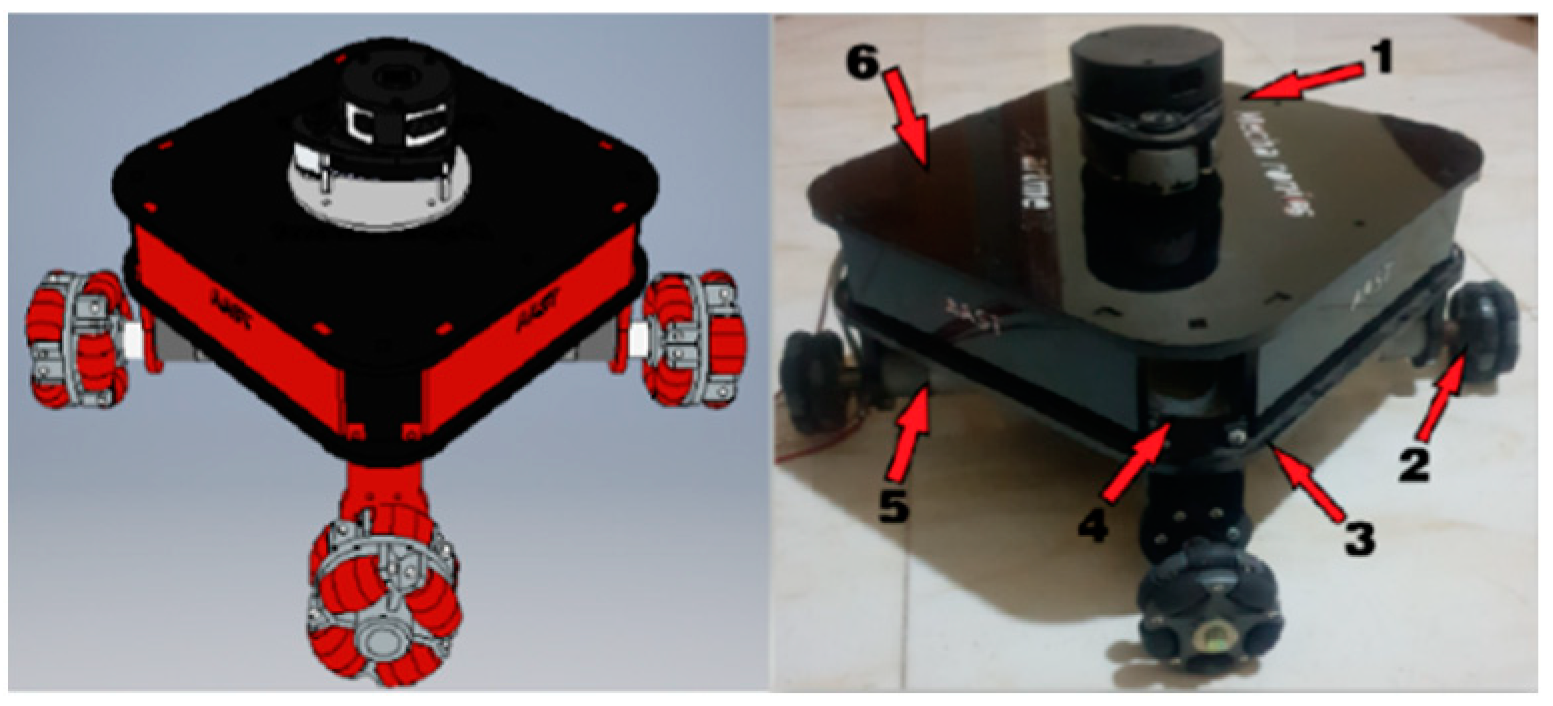
2. Specifications of the 4OWMR

The 4OWMR is based on four Omni-wheels with 90 degrees between each other. The wheels are located symmetrically at the corners of a square mobile platform base. The main body is constructed from a 6 mm acrylic sheet. The robot length, width and height are 360, 360, and 210 mm, respectively. The weight of the robot is approximately 3.5 kg. The robot’s wheel radius is 58 mm, and its wheel weight is 0.06 kg. It can reach a maximum velocity of 0.3035 m/s. The robot is also equipped with a Lidar sensor with a range of 12 m for navigation and creating occupancy maps. All components are shown in Figure 1 with annotations. The design is characterized by simplicity in assembly and disassembly, In addition to the robot’s modularity and the easiness of accommodation of its internal components.

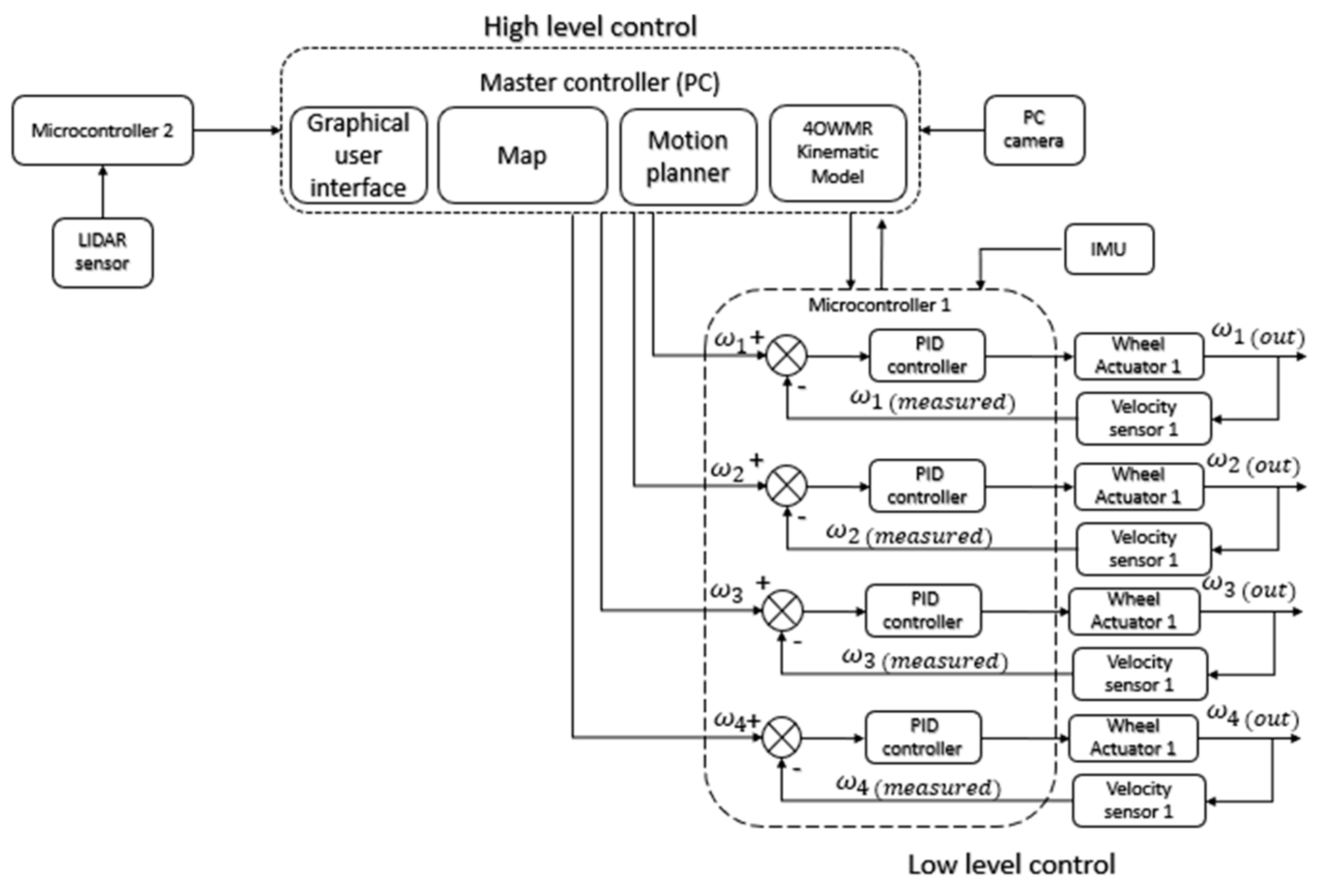
3. Control System of the 4OWMR

The implemented control scheme of the omni-wheel mobile robot is divided into two main stages (low-level and high-level stages). The schematic overview that describes the control stages is shown in Figure 2. The main functions of each stage are stated in the following subsections.

3.1. Low-Level Control

The first one, the low-level control stage, controls the velocity and position of each wheel and sends essential feedback data to the master controller. The position and the velocity of the mobile robot are determined using encoders and IMU sensor readings. The kinematics of the robot is calculated to determine the velocity and direction of the robot as a whole. The reference velocity and direction values are obtained using a non-linear PID controller. This controller communicates with the master controller (PC) using serial communication. This controller is considered responsible for the perception of the robot.

3.2. High-Level Control

The high-level controller is responsible for localization and planning the required path of the robot. It is equipped with a GUI interface enabling the user to choose the intended algorithm and follow the robot through the PC camera. The path planning algorithm is chosen and implemented on the robot to reach its destination. An online map of the robot’s environment is generated using LIDAR readings and updating the controller with the current location of the robot. Also, the camera feed is used to visualize the routes of the mobile robot. The robot kinematic model calculates the required angular velocities of the wheels and sends them to the low-level control stage. The implementation path planning algorithms are explained in detail in the following section. The main hardware components of the system are shown in

Table 2. Main hardware components of the omni-wheeled mobile robot (4OWMR).

Component Name	Specifications	Number
Lidar sensor	2D laser scanner Scan angle: 360 deg Range: 12 m Sampling points: 1450 points/scan Frequency: 10 Hz	1
Magnetic encoder	Resolution: 360 step/deg	4
Inertial Measurement Unit (IMU)	MPU9250 9-axis IMU	1
Microcontroller	Arduino Mega 2560	2
Master controller (PC)	Processor: i5-9500 CPU Ram: 8 GB	1
Wireless module	APC 220 kit RF	1
Omni wheels	Diameter: 58 mm Roller: 13 mm Material: Nylon	4

.

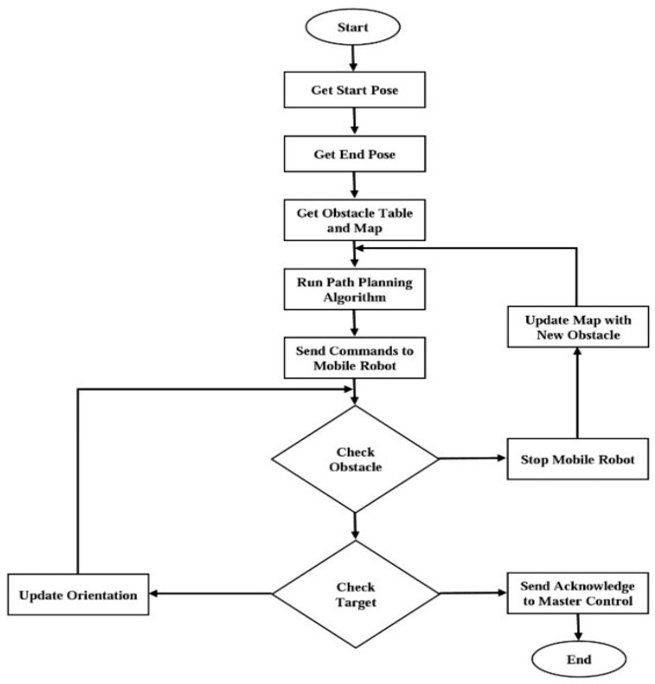
4. Proposed Path Planning Techniques

Path planning is defined as a process of determining a path in configuration space between the initial and target position of the robot [30]. The generated path should maintain the kinematic constraints of the mobile robot.

Indeed, the robot should not collide with obstacles (static or dynamic). Path planning can be classified into two types: Global path planning and local navigation path planning. In global path planning, prior knowledge of the environment (updated map and static obstacles) should be available. Many methods have been developed for global path planning, such as the A* algorithm [31], Cell decomposition method [32], RRT (Rapidly exploring Random Tree) and RRT* [33], and PRM (Probabilistic Roadmaps) [34]. In local navigation, the motion and direction of the robot are controlled autonomously by using onboard sensors, like ultrasonic range finder sensors, LIDAR sensors, IMU sensors, infrared range sensors, and vision (camera) sensors, etc.

A flowchart is shown in Figure 3, in which the implementation of the path planning code is shown. The code is initialized by recording the start and end positions, and it scans for the offline map. After that, the intended algorithm is calculated, and the desired path is generated and sent to the 4OWMR. If the robot faces an obstacle, it sends the data to the master controller, which stops the robot immediately while updating the map to generate a new path. If there is no new obstacle, the robot goes to a second check that checks if the robot has reached the target or not. If no obstacle is found, the robot continuously moves according to generated path till it reaches the final destination.

Several algorithms are chosen for implementation on the 4OWMR. The PRM, RRT, RRT*, and A* algorithms are described theoretically, applied, and compared experimentally, and their results are enhanced by using the genetic algorithm optimization technique (GA), as can be seen in the later sections. The theoretical explanation for the path planning algorithms is explained in the following subsections.

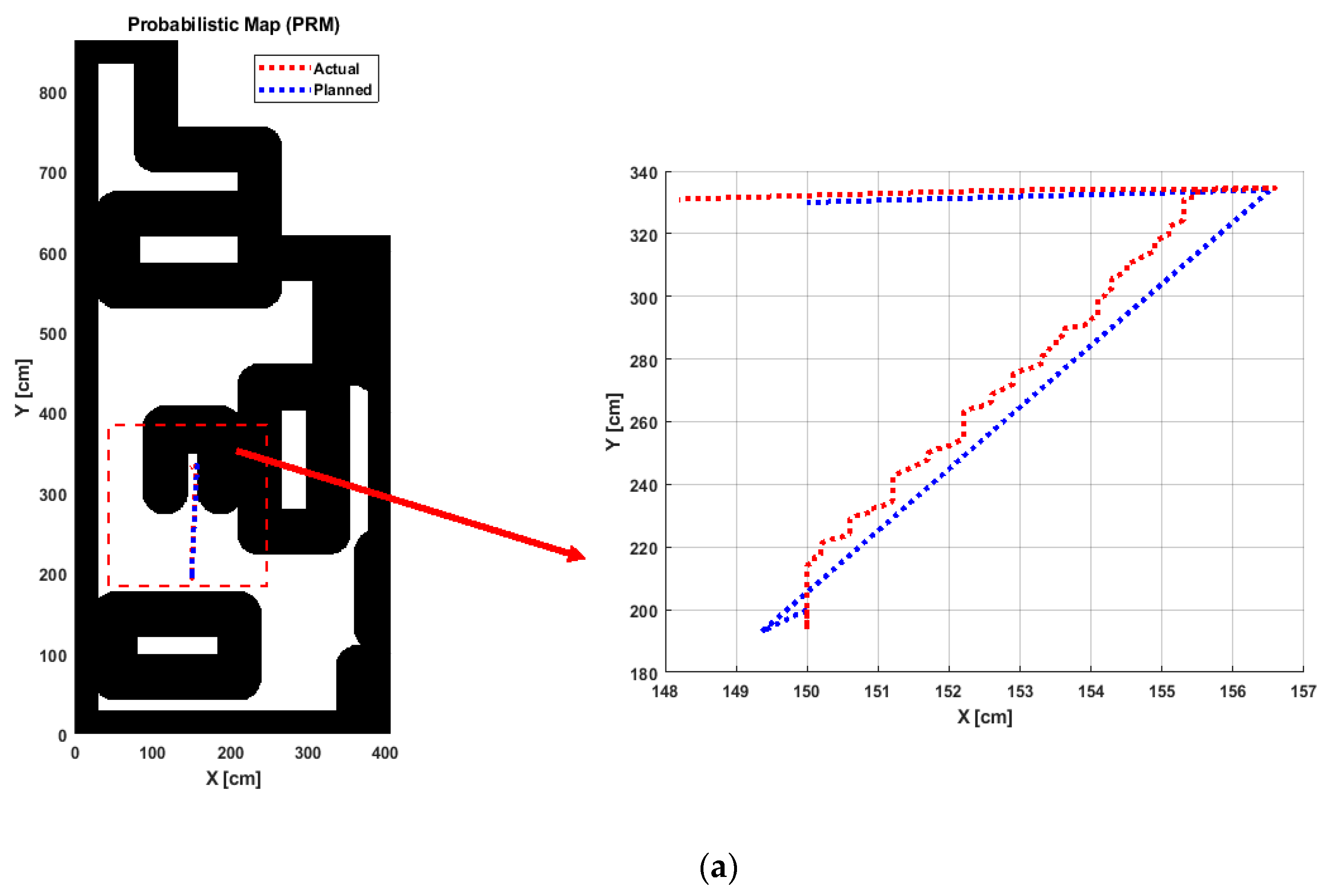
4.1. Probabilistic Roadmaps (PRM) Algorithm

The PRM algorithm is primarily used for multi-query applications. It consists of two main phases:

• Preprocessing Phase: In this phase, a graph (road map) noted (G) is generated. It is accessible from every point of the free configuration space $C_{free}$;
• Query Phase: The two points $q_s$ (start point) and $q_G$ (final point) are given. The sequence of edges that forms the required path is obtained from $q_s$ to $q_G$.

In the preprocessing phase, the generation of a road map is the main task of the preprocessing phase. The input is the number of iterations, and the number of nearest neighbors and the output is PRM G. G (V, E) represents a topological graph in which V is a set of vertices and E is the set of paths that map into $C_{free}$.

The algorithm initializes the vertices set and edges set by the empty set. In each iteration, while the absolute number of vertices is less than the number of samples, the algorithm selects a random point $q$ from configuration space. Then it checks whether $q$ ∈ $C_{free}$ or not (line 4). Once $q$ ∈$C_{free}$, it is inserted as a vertex of G. The pseudocode for this algorithm is shown in the following pseudocode.

Input: Number n of samples, number k of nearest neighbors   Output: PRM G = (V, E)

1:  initialize V = ∅, E = ∅ 2:  while |V| < n do    //find n collision-free points qi 3:      q ← random sample from C 4:      if q ∈ Cfree then V ← V ∪ {q} 5:  end while 6:  for all q ∈ V do  //check if near points can be connected 7:    Nq ← k nearest neighbors of q in V 8:    for all q′ ∈ Nq do 9:      if path (q, q′) ∈ Cfree then E ← E ∪ {(q, q′)} 10:    end for 11:       end for

The next step is to try to connect q to some nearby vertices G. The algorithm checks the path from q to q’ to see if it can be constructed or not; if yes, the set of edges will be increased by a new edge [35].

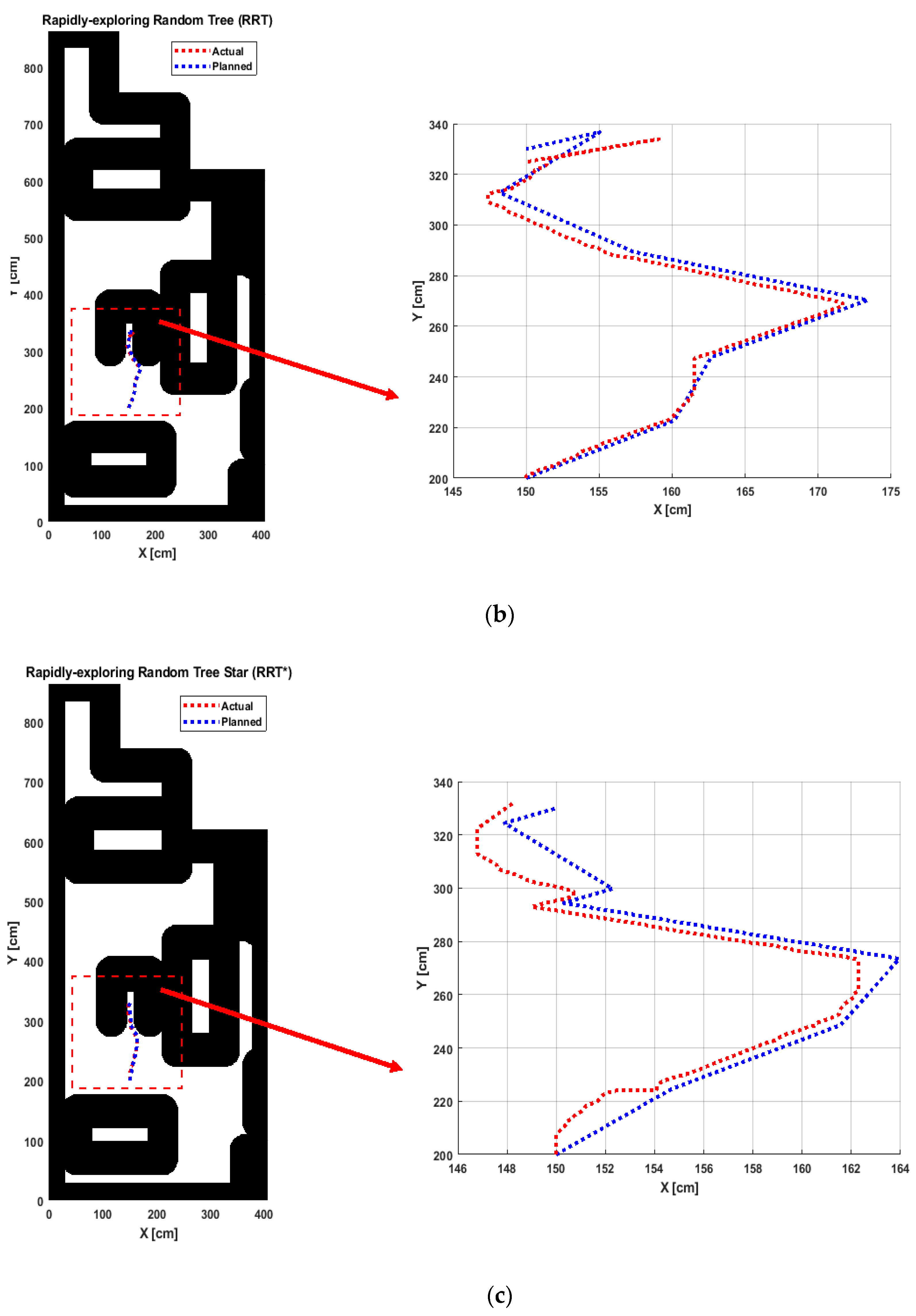
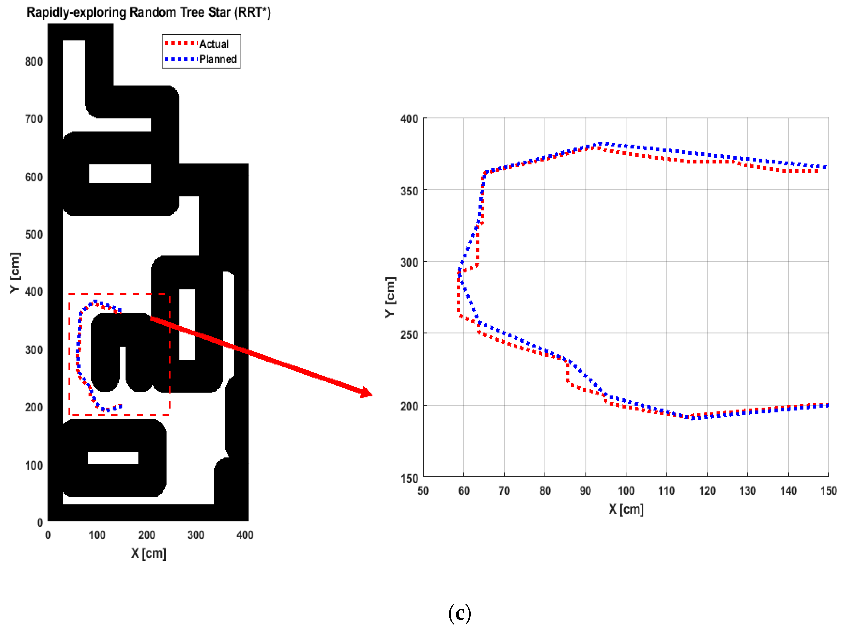
4.2. RRT (Rapidly exploring Random Tree) and RRT* Algorithms

The secondly implemented algorithm is the rapidly exploring random tree (RRT) algorithm [36]. It is used for single-query applications. The algorithm builds a tree of feasible trajectories rooted at the initial vertex. The algorithm is explained in pseudocode 2 and can be summarized as follows:

Input: $q_I,$ n of nodes, step size $\mathsf{\alpha }$   Output: Tree T = (V, E)   initialize V = {$q_S$}, E = ∅

1:  for i = 0: n do 2:    $q_{i }$ ← random sample from C 3:    $q_{near }$← nearest neighbor of qi in C 4:    $q_{new}$← $q_{near }$ + $\frac{\mathsf{\alpha }}{\left|q_i-q_{near}\right|} \left(q_i-q_{near}\right)$ 5:    if $q_{new}$∈ $C_{free}$then V ← V ∪{$q_{new}$}, E ← E ∪ {( $q_{near }$, $q_{new}$)} 6:  end for

Many derivatives of RRT algorithms are present and sought after. The most common derivative is the RRT* [37], which will be implemented on the 4OWMR.

4.3. Hybrid A* Algorithm

This path-planning algorithm is one of the most efficient path-planners for mobile robots or autonomous vehicles [38]. It consists of two parts; the first one is named the forward search stage. The algorithm is guided by a cost function named g(n); it works from the starting node to the current node (n). It has two more functions named ${\mathrm{h}}_1\left(n\right)$ and ${\mathrm{h}}_2\left(n\right)$ respectively. ${\mathrm{h}}_1\left(n\right)$ is a heuristic function that uses the obstacle map to compute the cost of the distance from the current node to the goal in the discrete state. Another heuristic function named ${\mathrm{h}}_2\left(n\right)$ which considers the kinematics of the used mobile robot. The robot kinematics is used to predict the path that considers the direction, steering angle and speed of the mobile robot in the continuous state. Then, the algorithm selects the right successor in continuous coordinate and lets the mobile robot follow it. The overall objective function of the planner algorithm at each node n is shown in Equation (3).

$$F\left(n\right)=g\left(n\right)+{\mathrm{h}}_1\left(n\right)+{\mathrm{h}}_2\left(n\right)$$

(1)

The second stage is called analytic expansion, which ensures that the algorithm achieves the continuous coordinate of the goal state.

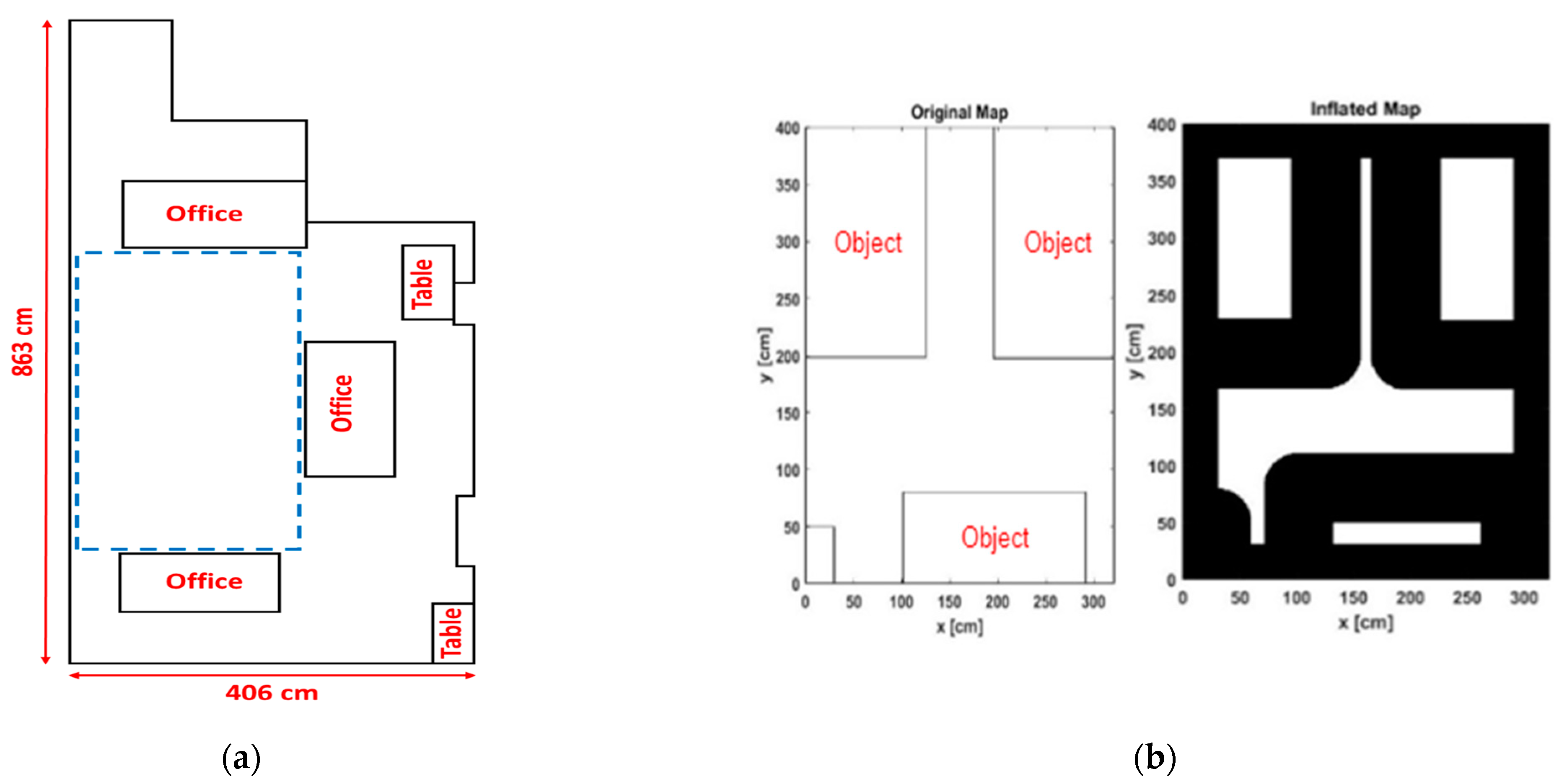
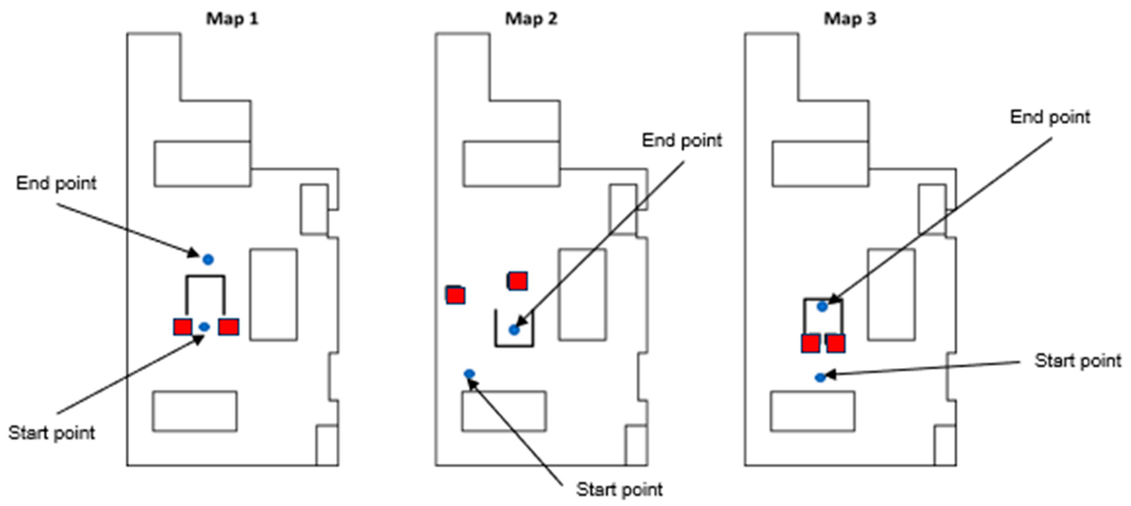
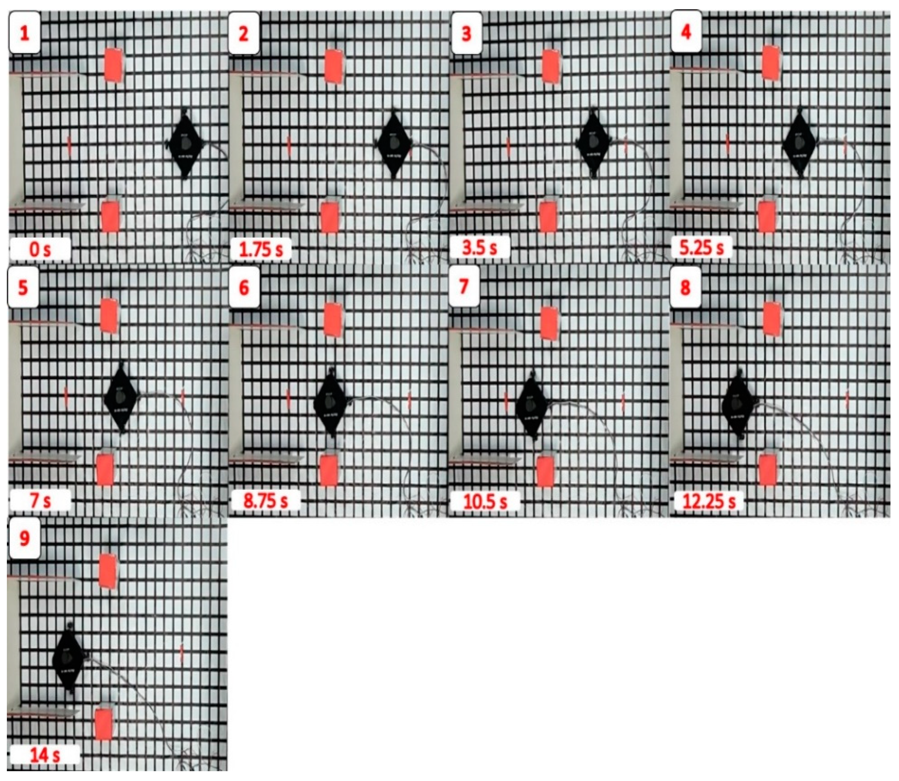
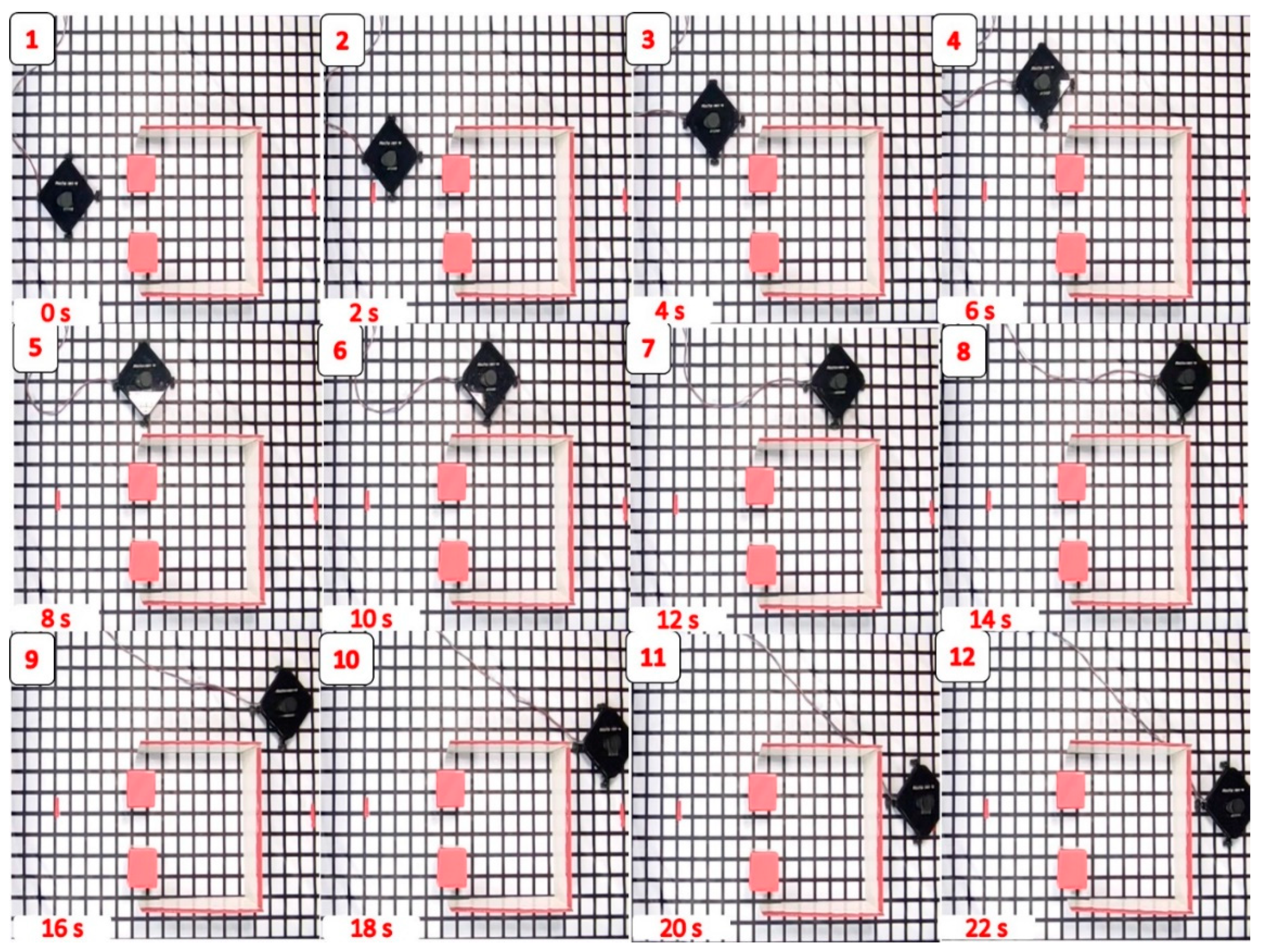
5. Experimental Implementation and Results

In order to examine the robot navigation experimentally, an indoor office room is chosen. The dimensions of this room are 863 cm × 406 cm. The blue rectangle, which is shown in Figure 4a, is the working area of the 4OWMR. The working area is divided into small squares 10 cm × 10 cm for capturing the actual path. Different static obstacles are added to this map in different configurations to test the robot’s maneuverability and the applied path-planning technique.

Inflated maps are often used to apply a protection element to obstacles and build buffer areas between the robot and the environment’s obstacles. It is built into the robot software before path generation. An example of inflated maps that are used in the software is shown in Figure 4b. Local path planning is utilized in the following experiments such that the map obstacles placement is unknown. Three different maps (denoted Map1, Map2 and Map3) are used as examples for validation. These maps are shown in Figure 5.

The generated paths are additionally optimized by using a multi-objective genetic algorithm [39] to minimize the path length and the number of turns of the 4OWMR. The multi-objective optimization problem is converted to a single-objective optimization process by using a weighted sum, as shown in Equation (2).

$$fitness=\left(A\times f_1\right)+\left(B\times f_2\right)$$

(2)

where A + B = 1, $f_1$ = 1/path and $f_2$ = C/S

$fitness$ is the total fitness function, $f_1$ is the fitness function of the path length, $f_2$ is the fitness function of path smoothness, and A and B are the weights of the two fitness functions. C is the precision coefficient, and S is the smoothness of the path. $f_1$, $f_2$, and C are controlled to maintain the same magnitude order.

The fitness function’s responsibility is to rank the chromosomes for the motion problem. Any specific path would be composed of n waypoints. Hence, the path length is expressed as $path,$ as shown in Equation (3).

$$path={⅀}_{i=1}^{n-1}\sqrt{(x_{i+1}-x_i{)}^2+(y_{i+1}-y_i{)}^2 }$$

(3)

Additionally, other optimization parameters are as follows; the initial population size is 800. The stopping criteria are when the first acceptable solution is sought, continues for a predetermined number of iterations, and then stops. The maximum number of generations is the maximum number of successful iterations, which is 50 generations.

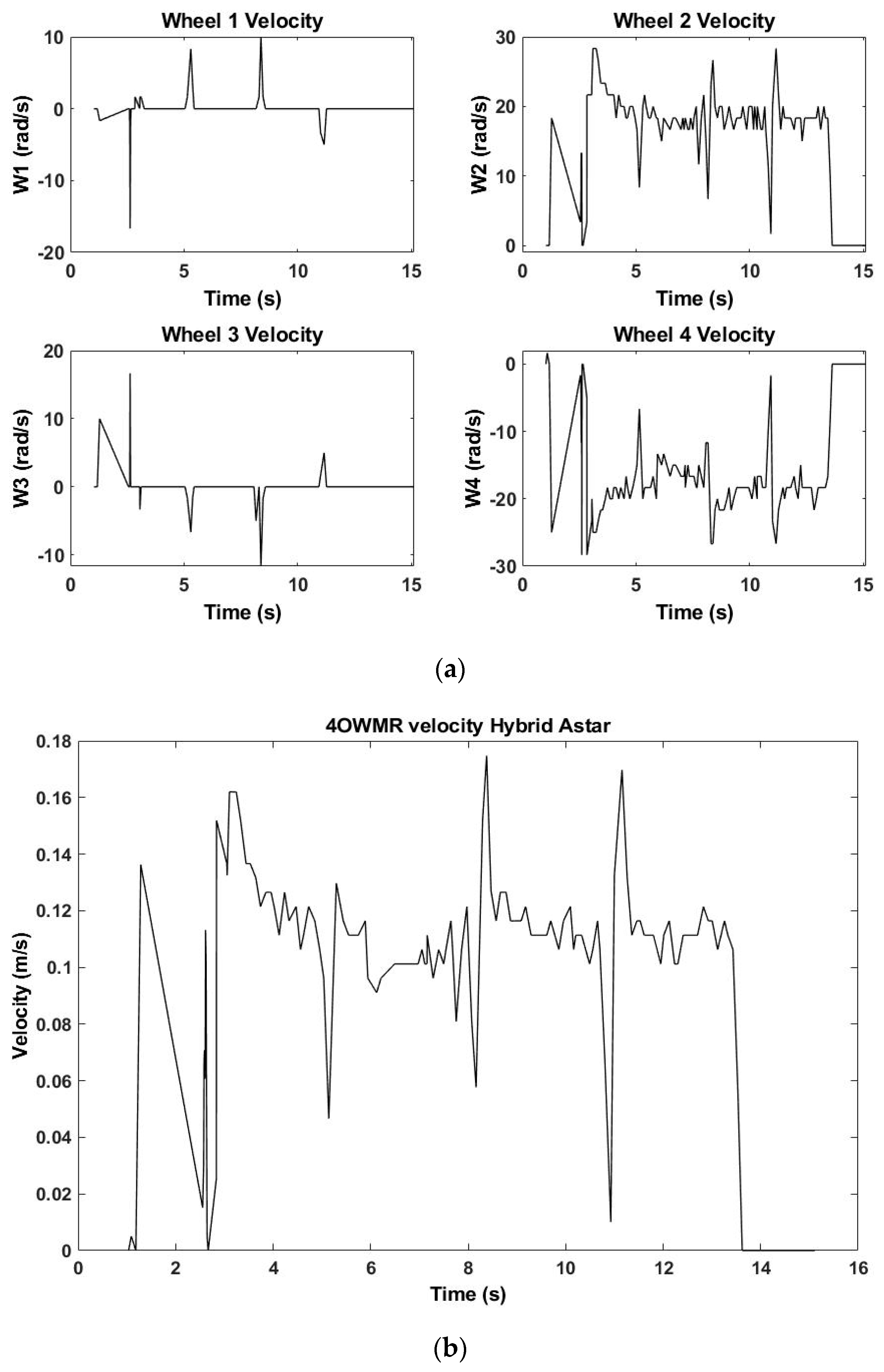
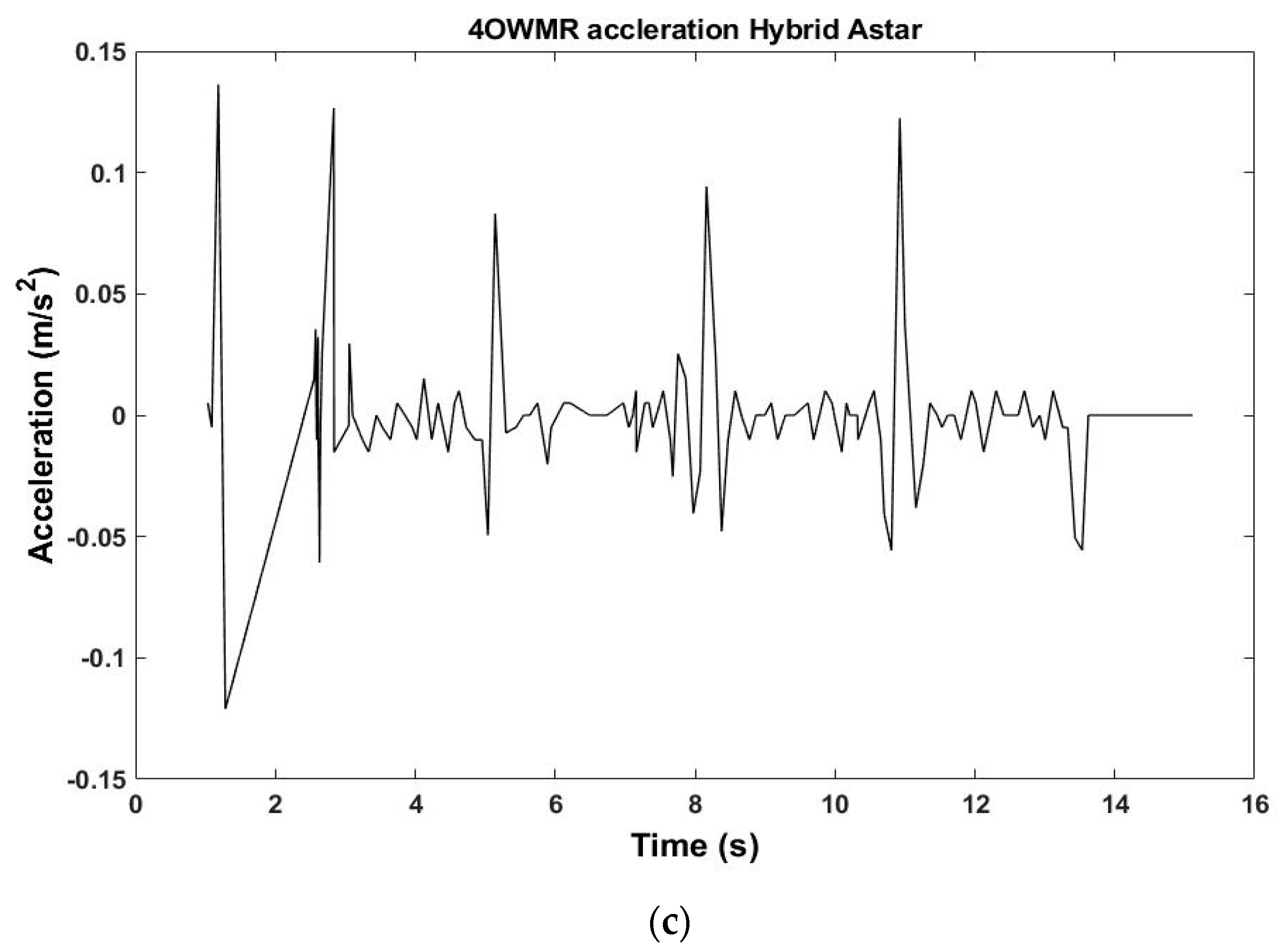
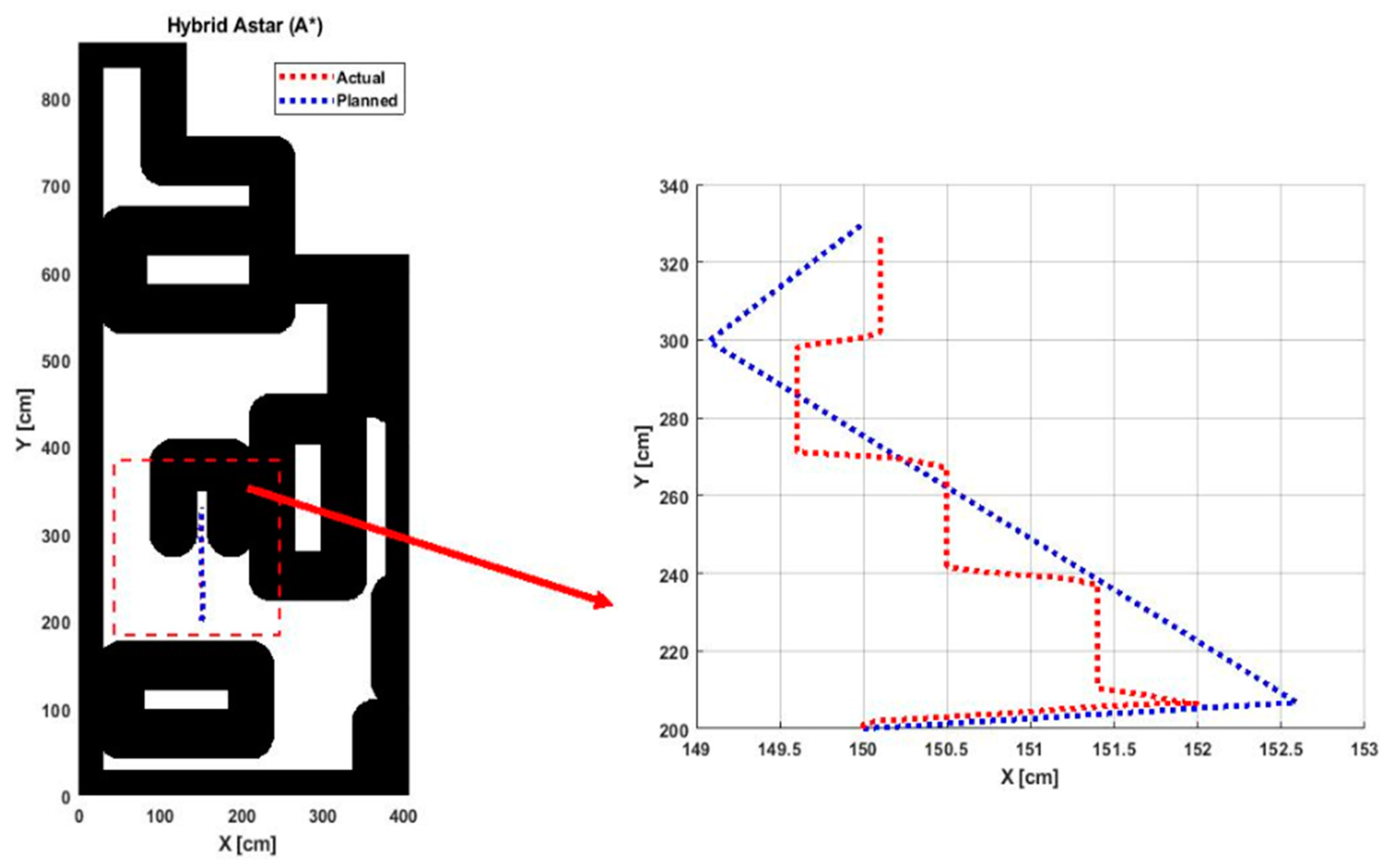
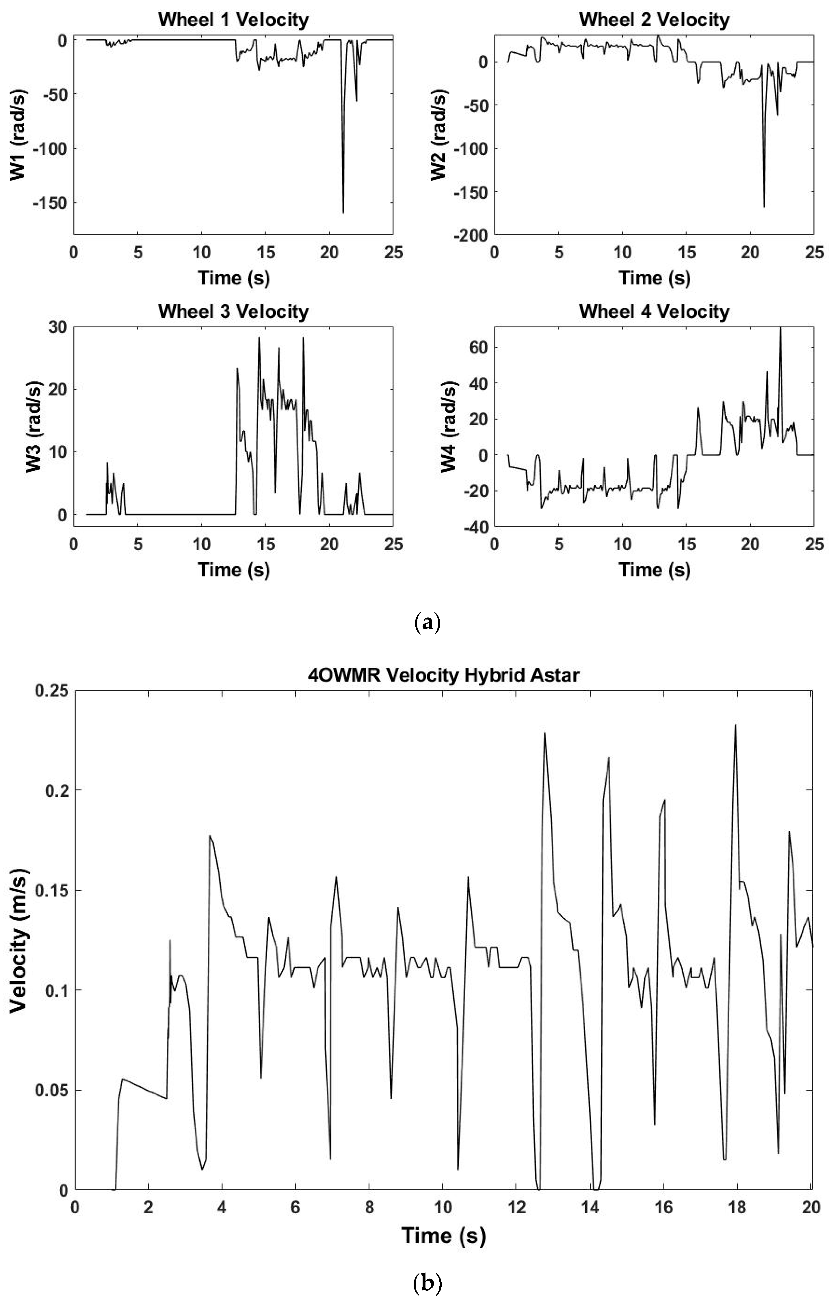
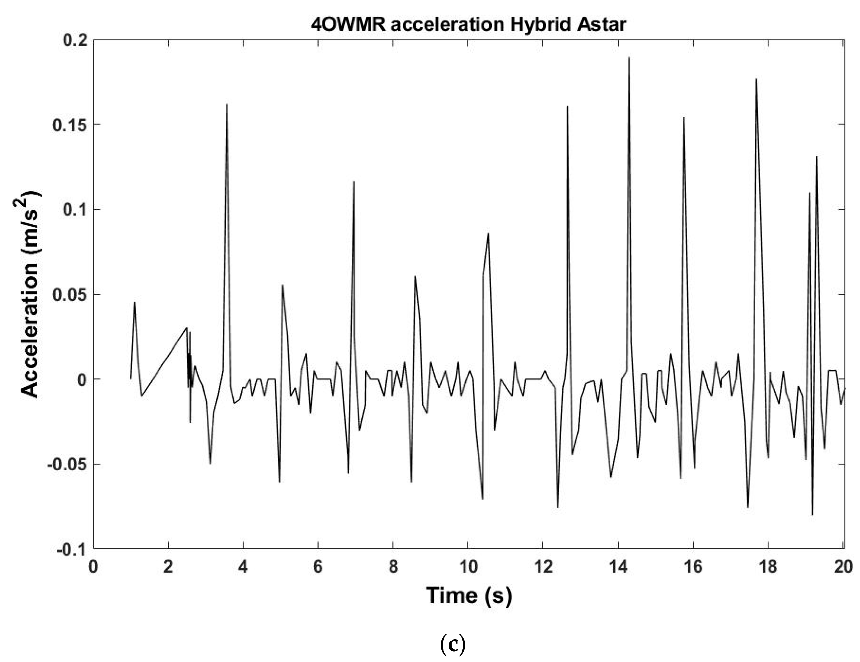
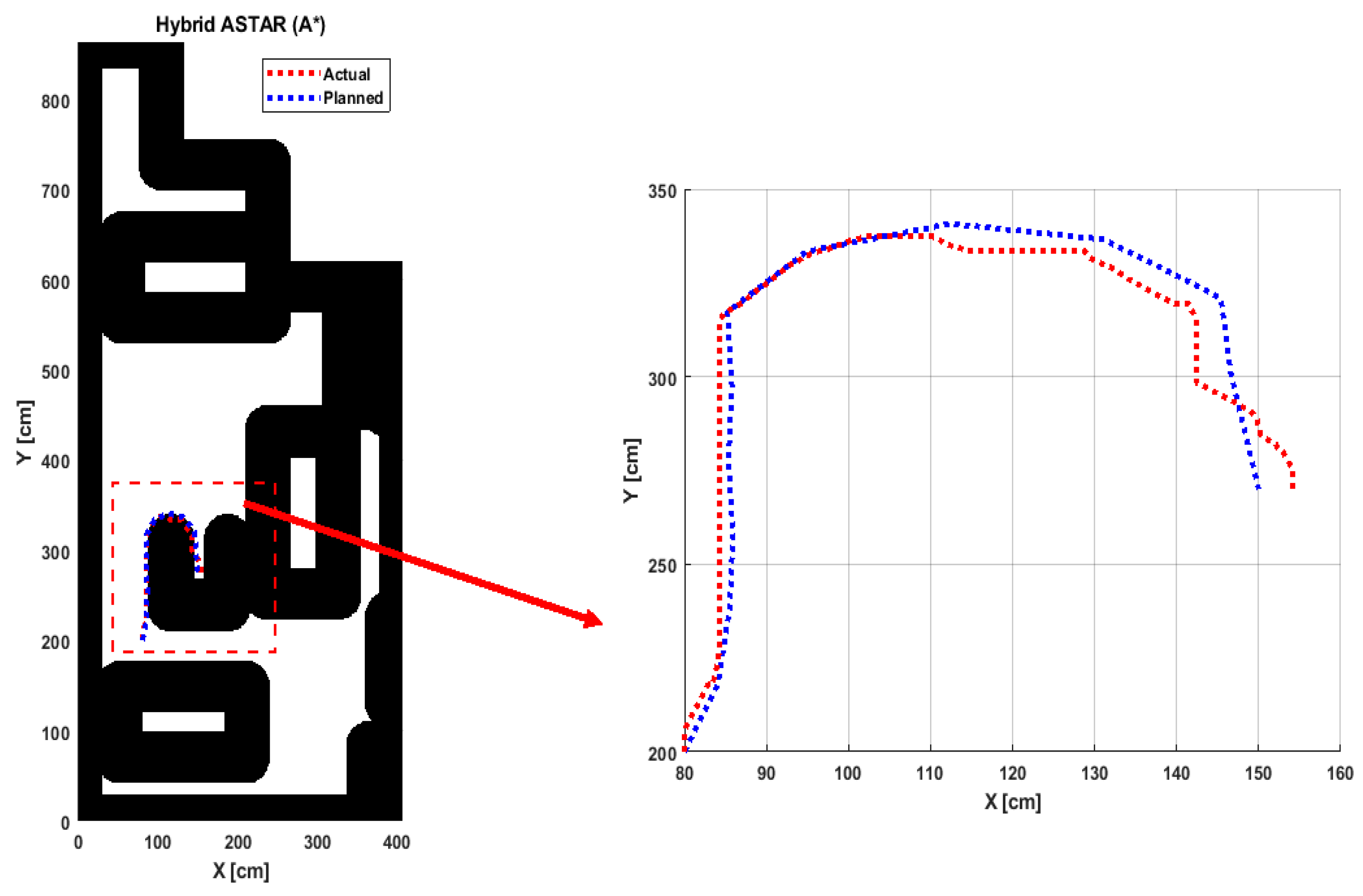
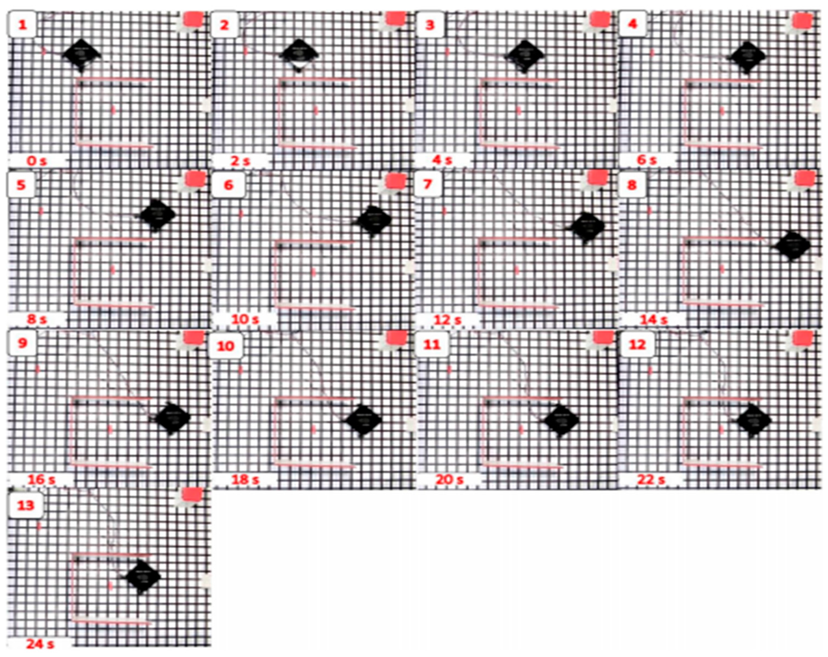
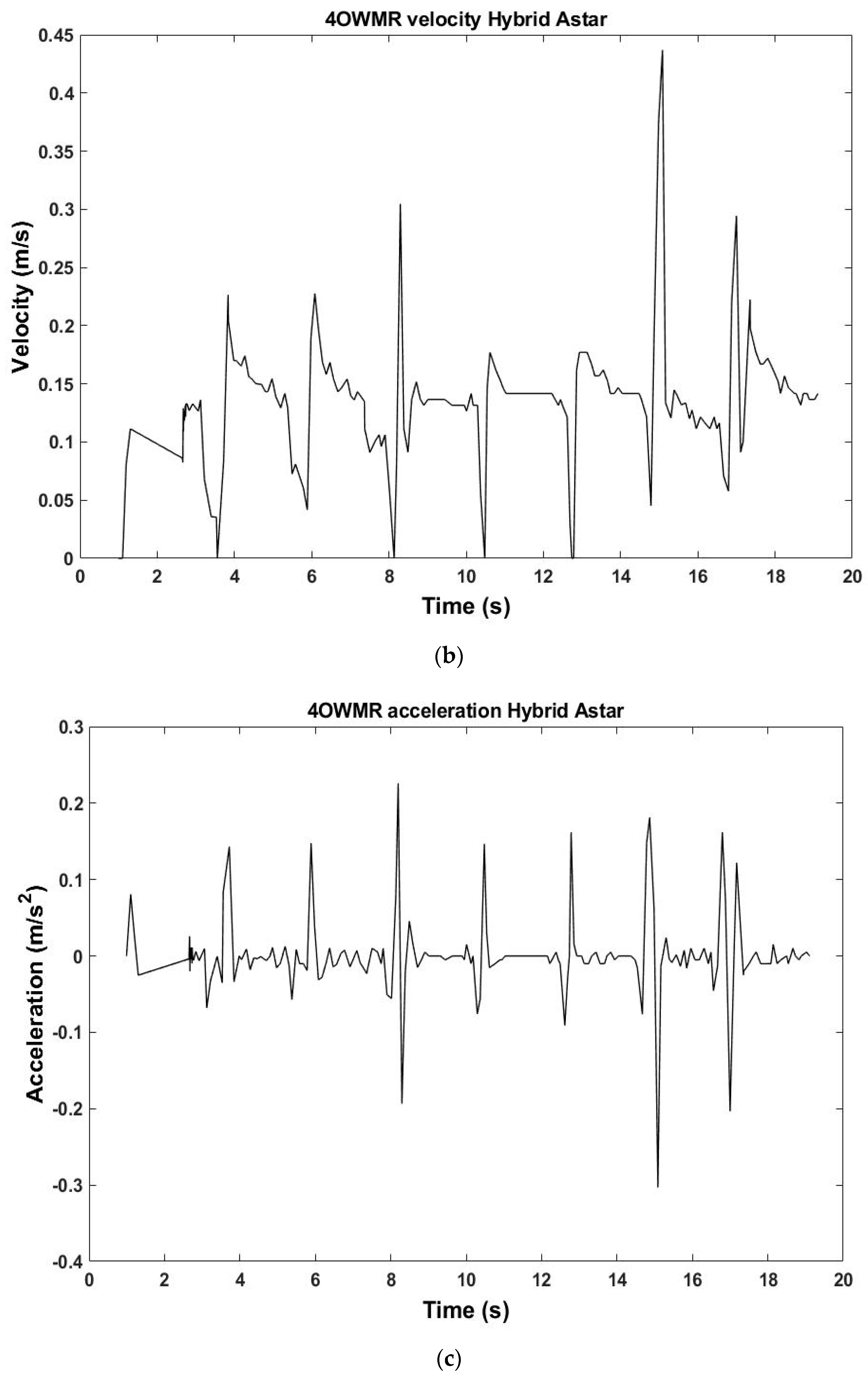
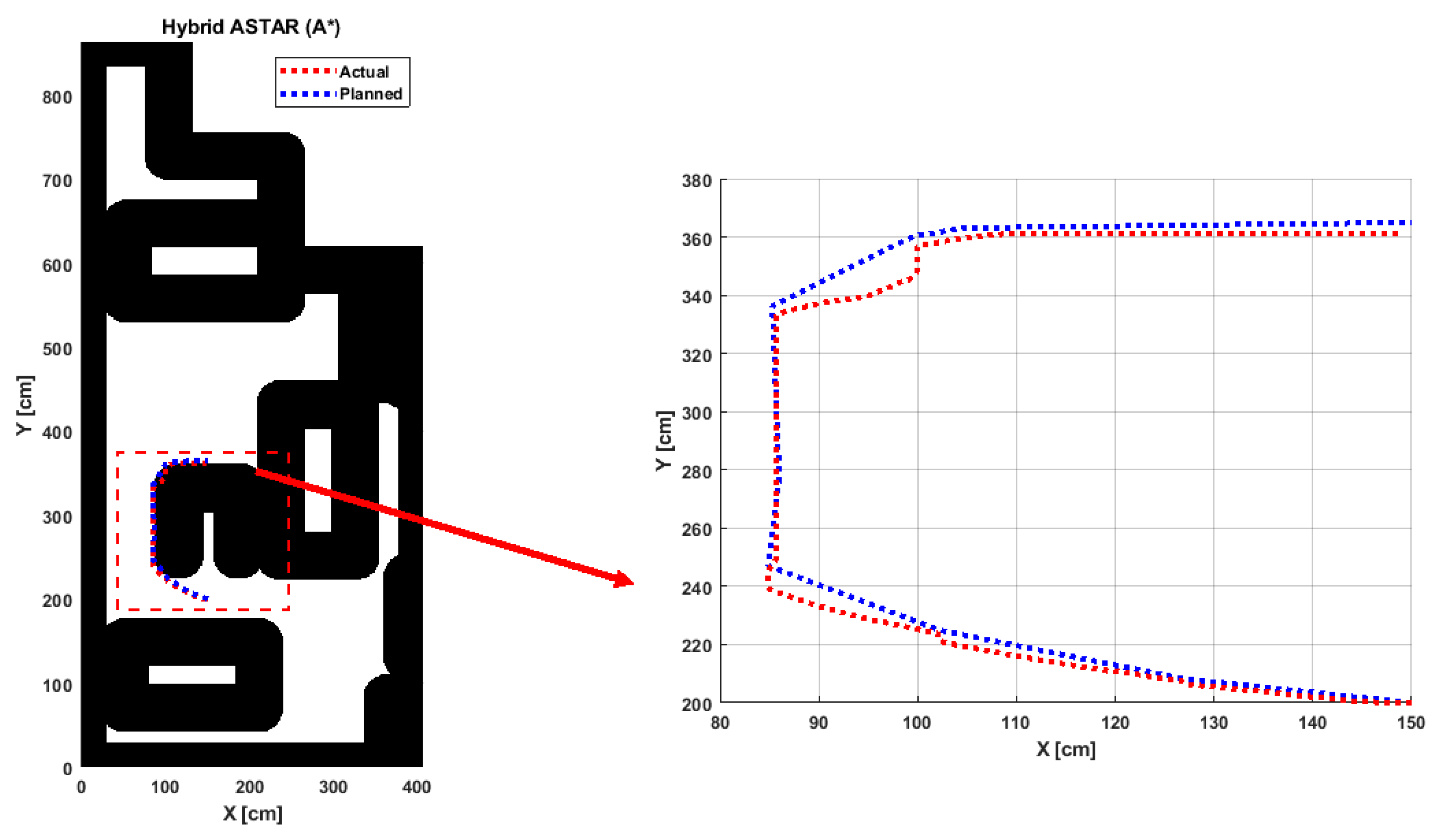
5.1. Experimental Hybrid A* Results for Map1

The velocity of each wheel is shown in Figure 6a, and then inverse kinematics is computed for generating the total mobile robot speed, as shown in Figure 6b. Then, Figure 7 presents the planned path (blue path) generated from algorithms and the actual path (red Path) traveled by the mobile robot. The experimental path of the mobile robot in Map1 can be presented as a series of images, as shown in Figure 8.

The generated path has a travel distance = 1.31 × 10² cm, an average velocity of 0.1189 m/s, a travel time of 13.621 s and a maximum acceleration of 0.141 m/s². The real final point is varied from the planned as the absolute error point on the X- and Y-axes and is 0.3 cm and 2.1 cm, respectively.

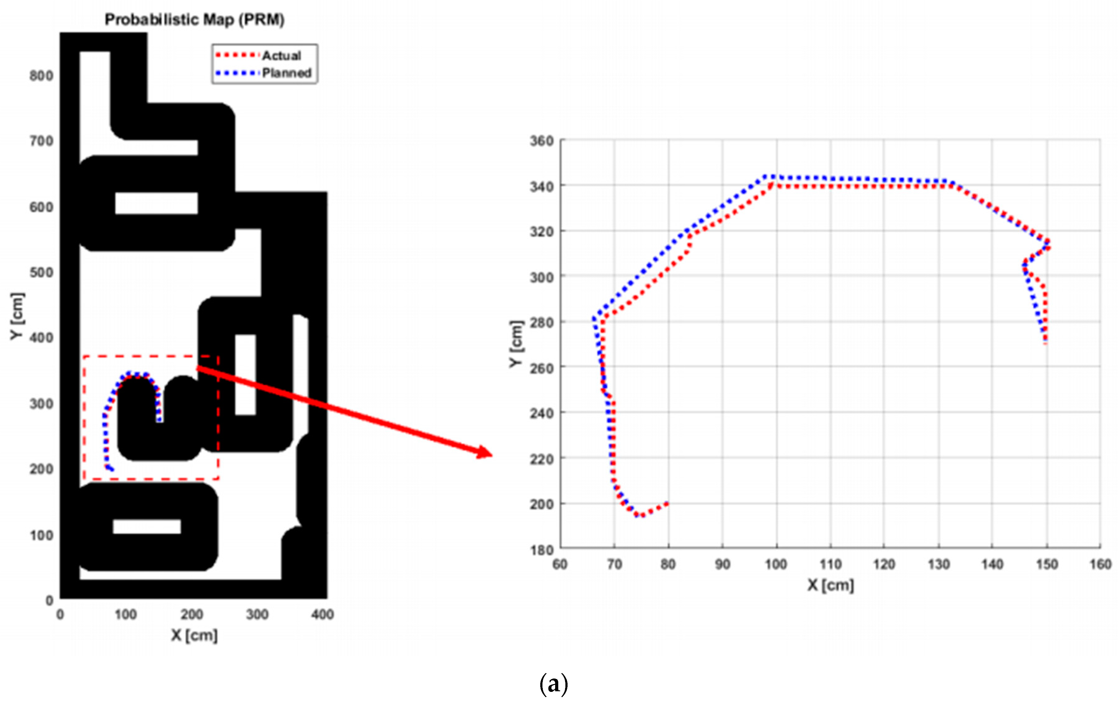
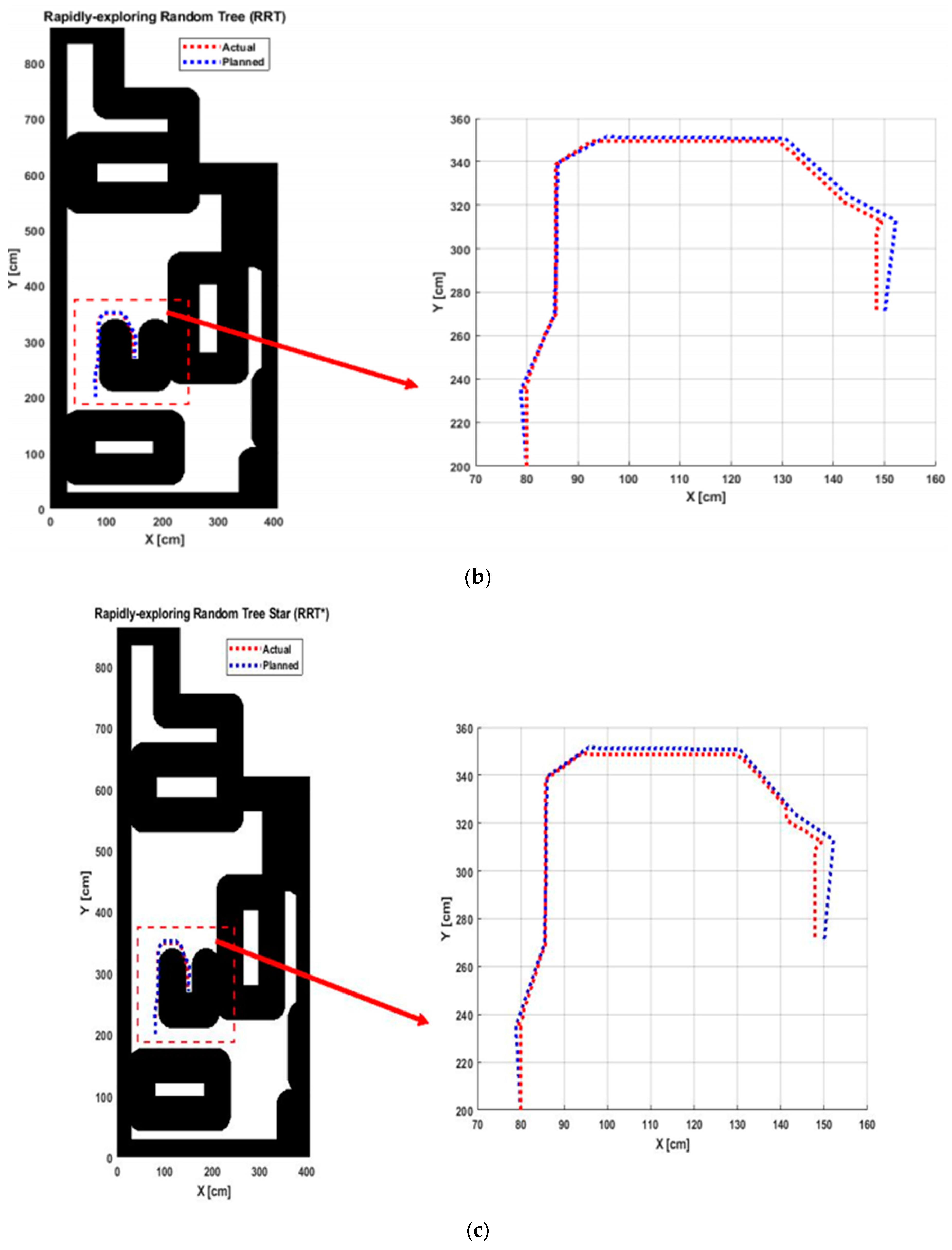
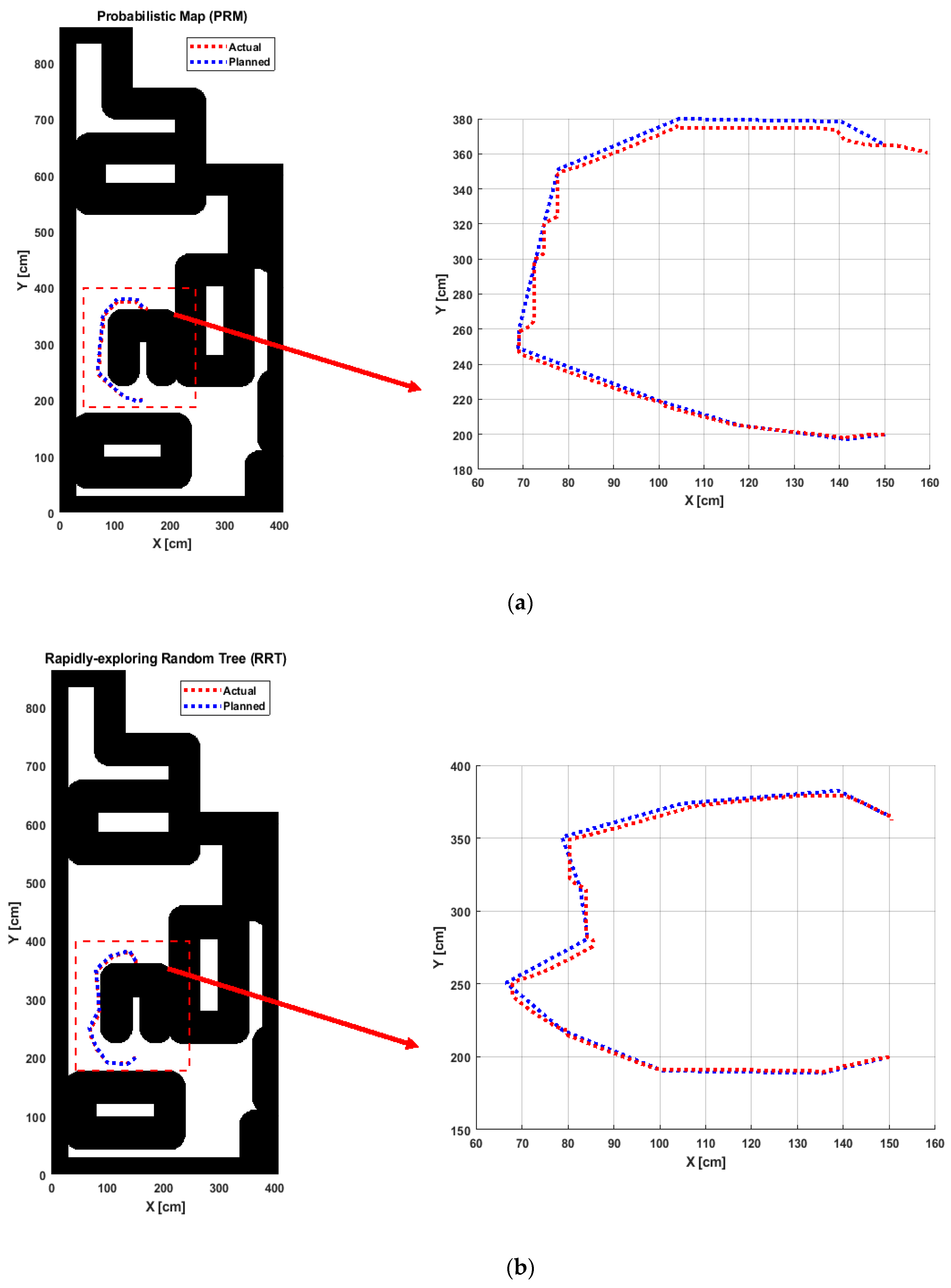
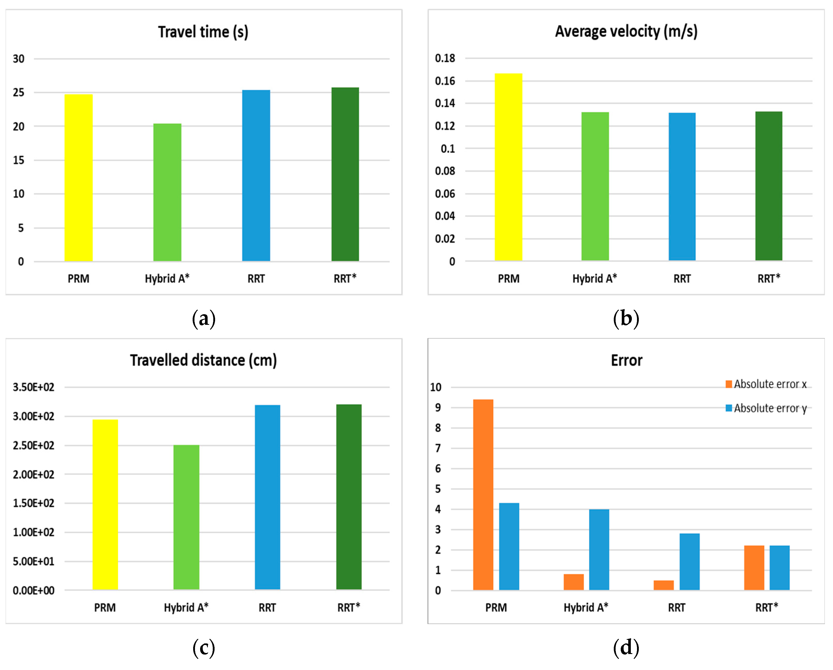
5.2. Experimental PRM, RRT and RRT* Results for Map1

PRM, RRT and RRT* algorithms are also applied on this map, and the generated paths are shown in Figure 9. The measured experimental values like traveled distance, average velocity, travel time, and absolute error (x, y) are shown in Figure 10.

5.3. Experimental Hybrid A* Results for Map2

The velocity of each wheel is shown in Figure 11a, and then inverse kinematics is computed for generating the total mobile robot speed, as shown in Figure 11b. Then, Figure 12 presents the planned path (blue path) generated from algorithms and the actual path (red Path) traveled by the mobile robot. The experimental path of the mobile robot in Map2 can be presented as a series of images, as shown in Figure 13.

The generated path has a travel distance = 2.47 × 10² cm, an average velocity of 0.1106 m/s, a travel time of 23.62 s and a maximum acceleration of 0.192 m/s². The real final point is varied from the planned as the absolute error point on the X- and Y-axes and is 4.2 cm and 0.9 cm, respectively.

5.4. Experimental PRM, RRT and RRT* Results for Map2

PRM, RRT and RRT* algorithms are also applied on this map, and the generated paths are shown in Figure 14. The measured experimental values like traveled distance, average velocity, travel time, and absolute error (X, Y) are shown in Figure 15.

5.5. Experimental Hybrid A* Results for Map3

The velocity of each wheel is shown in Figure 16a, and then inverse kinematics is computed for generating the total mobile robot speed, as shown in Figure 16b. Then, Figure 17 presents the planned path (blue path) generated from algorithms and the actual path (red path) traveled by the mobile robot. The experimental path of the mobile robot in Map3 can be presented as a series of images, as shown in Figure 18.

The generated path has a travel distance = 2.51 × 10² cm, an average velocity of 0.1321 m/s, a travel time of 20.44 s and a maximum acceleration of 0.325 m/s². The real final point is varied from the planned as the absolute error point on the X- and Y-axes and is 0.8 cm and 4 cm, respectively.

5.6. Experimental PRM, RRT and RRT* Results for Map3

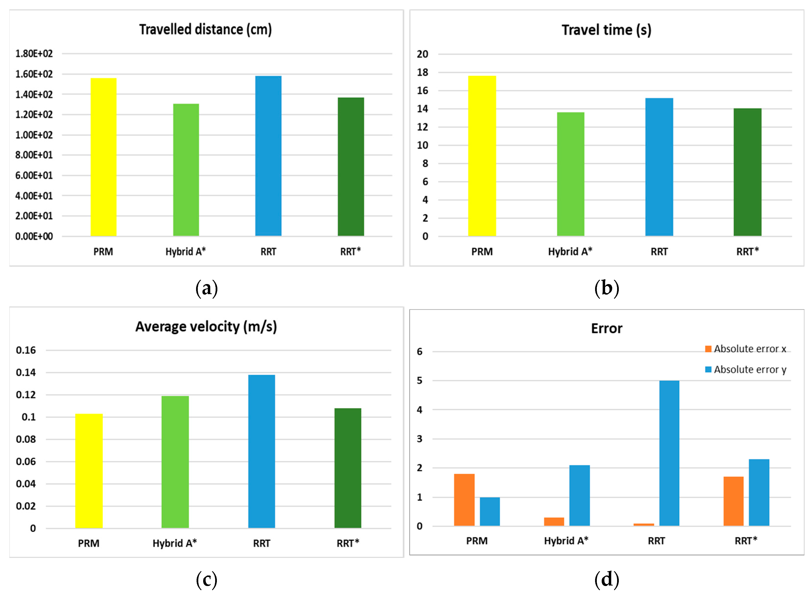
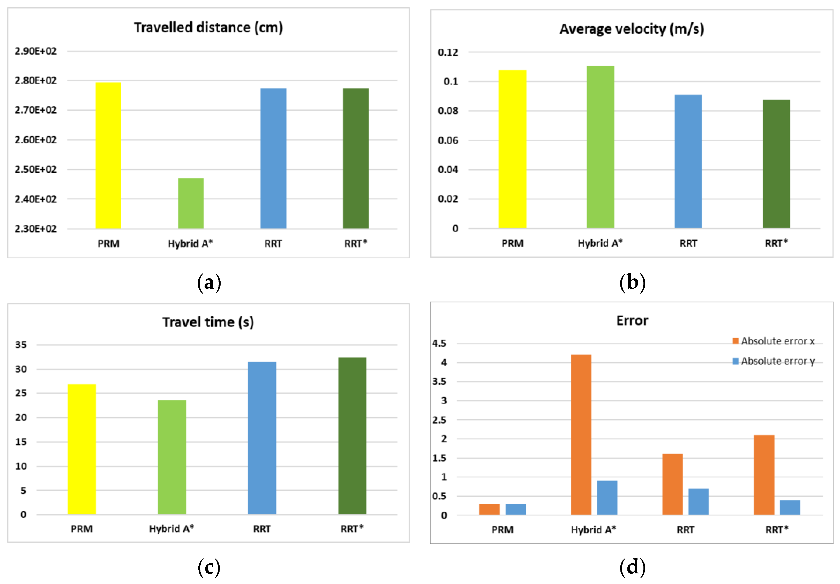
PRM, RRT and RRT* algorithms are also applied on this map, and the generated paths are shown in Figure 19. The measured experimental values like traveled distance, average velocity, travel time, and absolute error (X, Y) are shown in Figure 20.

6. Discussion

Based on the previous results, the applied algorithms are compared to select the most convenient path-planning technique for the 4OWMR. A multi-criteria decision-making method named weighted sum [40] is chosen. The general formula for the weighted sum is shown in Equation (4).

$$A_{WSM-score}^{*}=\max {⅀}_{j=1}^n{a}_{ij}{w}_j$$

(4)

where i = 1, 2, 3..., m

$A_{WSM-score}^{*}$ is the best choice score, n is the number of decision criteria, $a_{ij}$ is the actual value of the i^th alternative in terms of the j^th criterion, and $w_j$ is the ranking weight of the j^th criterion. The ranking is done on all results of all algorithms of all of the three available maps. The parameters that are ranked are the travel distance, average velocity, travel time, and absolute error in (x, y) coordinates. These parameters were given equal weights, and their ranking results for the three maps are displayed in

Table 3. The ranking table of the applied algorithms on three indoor maps.

Map Number	Method of Path Planning	Convergence Ranking	Energy Consumption Ranking	Overall Ranking
Map1	PRM Hybrid A* RRT RRT*	2 1 4 3	4 1 3 2	4 1 2 3
Map2	PRM Hybrid A* RRT RRT*	1 4 3 2	2 1 3 4	1 2 3 4
Map3	PRM Hybrid A* RRT RRT*	4 2 1 3	2 1 4 3	2 1 3 4

.

The main aim of this research is to present an experimental comparative study of different path-planning techniques for an indoor mobile robot. The results are ranked according to convergence rate, energy consumption and overall ranking. The convergence is represented by the absolute error in the x and y coordinates at the endpoint.

This error is calculated using Middle Difference in Distance Driven ($M_{DDD}$) as shown in equation 5, which is the total distance of the planned path generated from the algorithms. Time is the total time for driving the mobile robot from the start point to the goal point in the real environment, and Maximum Deviation is the maximum absolute difference between the real and the actual path. $M_{DDD}$ is calculated in all maps for all techniques and its results are ranked and presented in Table 3. The highest-ranking results in convergence are the RRT* technique followed by the Hybrid A*.

$$M_{DDD}=\frac{\frac{{{\displaystyle \sum }}_n^i(dis{t}_{actual}-dis{t}_{planned})}{dis{t}_{planned}}}{n}$$

(5)

where the $dis{t}_{actual}$ is the distance between two consecutive points in the actual path, $dis{t}_{planned}$ is the distance between two consecutive points in the real path, and $n$ is the number of distances in the real path.

The energy consumption ranking is based on travel distance, average velocity and travel time. In the three maps, the Hybrid A* is ranked first in energy consumption parameters. Consequently, Hybrid A* has the lowest cost among the other techniques and relatively high convergence in the three maps (but not the best). In other words, if average velocity, travel time and travel distance are given higher weights in the ranking process, the Hybrid A* would be the best choice for the 4OWM in indoor environments.

Moreover, the Hybrid A* avoids complexity in computation during real-time deployment. Another observation is that Hybrid A* considers the robot’s kinematics and geometry, so it doesn’t require the addition of inflated maps during path planning generation.

7. Conclusions and Future Work

In this paper, research efforts in this thesis have concentrated on the path planning of a mobile robot against unknown static obstacles. The work is presented experimentally in order to produce reliable results. A four omni-wheeled mobile robot (4OWMR) is used as the mobile platform to give simultaneous rotating and sideways motions, particularly in small spaces. To manage the robot during navigation and enable localization in indoor maps, low-level position and velocity control loops are used. To recognize the surrounding obstructions, a LIDAR sensor is included. During indoor navigation, a user interface (GUI) is designed to monitor the robot and use path-planning algorithms.

Local path planning is implemented with four path planning algorithms: PRM, hybrid A*, RRT, and RRT*. Optimization using a genetic algorithm is applied to the generated paths to improve the generated paths. Based on these trials, comparison research evaluating the performance of the 4OWMR in various environments is done in terms of success rate, velocity, travel distance, duration, and convergence absolute error. Hybrid A* is proven to be relatively better than the other algorithms while using the weighted sum ranking technique. In convergence ranking, the Hybrid A* is generally second in all maps (only behind RRT*). Also, it is ranked first in energy optimization rankings. The overall ranking results of the Hybrid A*, when compared to other techniques, are 81.67% against RRT, 80% (PRM), and 71.67% (RRT*).

For future work, more complicated and complex maps would be tested experimentally. Further optimization techniques would be implemented to obtain more optimized paths. In addition, the implementation of machine learning techniques would be sought after to provide smoother paths, lower energy consumption and higher accuracy in convergence. Several hardware modifications will be sought after to get smoother paths and avoid possible discontinuities in path generation and slow sampling rates. The utilization of faster programming languages like python will be investigated for future implementation.

References

1. Rubio, F.; Valero, F.; Llopis-Albert, C. A review of mobile robots: Concepts, methods, theoretical framework, and applications. Int. J. Adv. Robot. Syst. 2019, 16, 1–22. [Google Scholar] [CrossRef] [Green Version]
2. Crnokic, B.; Grubisic, M.; Volaric, T. Different Applications of Mobile Robots in Education. Int. J. Integr. Technol. Educ. 2017, 6, 15–28. [Google Scholar] [CrossRef]
3. Siegwart, R.; Nourbakhsh, I.R.; Scaramuzza, D. Introduction to Autonomous Mobile Robots; The MIT Press: Cambridge, MA, USA, 2011; pp. 11–46, ISBN-10: 0262015358. [Google Scholar]
4. Kanjanawanishkul, K. Omnidirectional wheeled mobile robots: Wheel types and practical applications. Int. J. Adv. Mechatron. Syst. 2015, 6, 289–302. [Google Scholar] [CrossRef]
5. Shabalina, K.; Sagitov, A.; Magid, E. Comparative Analysis of Mobile Robot Wheels Design. Proc. Int. Conf. Dev. eSystems Eng. DeSE 2019, 2018, 175–179. [Google Scholar] [CrossRef]
6. Parmar, J.J.; Savant, C.V. Selection of Wheels in Robotics. Int. J. Sci. Eng. Res. 2014, 5, 339–343. [Google Scholar]
7. Oliveira, H.P.; Sousa, A.J.; Moreira, A.P.; Costa, P.J. Dynamical models for omni-directional robots with 3 and 4 wheels. In Proceedings of the ICINCO 2008—5th International Conference on Informatics in Control, Automation and Robotics, Milan, Italy, 2–5 July 2009; Volume 1, pp. 189–196. [Google Scholar]
8. Röhrig, C.; Heß, D. Omniman: An omnidirectional mobile manipulator for human-robot collaboration. In Proceedings of the International MultiConference of Engineers and Computer Scientists 2019, Hong Kong, China, 13–15 March 2019; Volume 2239, pp. 55–60. [Google Scholar]
9. Zhang, Y.; Guo, L.; Zhang, M.; Lv, X. Structure Design and Kinematics Analysis of Omni-Directional Mobile Platform. In Proceedings of the 2018 IEEE 8th Annual International Conference on CYBER Technology in Automation, Control, and Intelligent Systems (CYBER), Tianjin, China, 19–23 July 2018; pp. 1062–1067. [Google Scholar] [CrossRef]
10. Takahashi, M.; Suzuki, T.; Shitamoto, H.; Moriguchi, T.; Yoshida, K. Developing a mobile robot for transport applications in the hospital domain. Robot. Auton. Syst. 2010, 58, 889–899. [Google Scholar] [CrossRef]
11. Sofwan, A.; Mulyana, H.R.; Afrisal, H.; Goni, A. Development of Omni-Wheeled Mobile Robot Based-on Inverse Kinematics and Odometry. In Proceedings of the Information Technology, Computer and Electrical Engineering. International Conference, 6th 2019 (ICITACEE 2019), Semarang, Indonesia, 26–27 September 2019; pp. 143–148. [Google Scholar] [CrossRef] [Green Version]
12. Riaz, Z.; Pervez, A.; Ahmer, M.; Iqbal, J. A fully autonomous indoor mobile robot using SLAM. In Proceedings of the 2010 International Conference on Information and Emerging Technologies (ICIET 2010), Karachi, Pakistan, 14–16 June 2010; pp. 1–6. [Google Scholar] [CrossRef]
13. Patle, B.; Pandey, A.; Parhi, D.; Jagadeesh, A. A review: On path planning strategies for navigation of mobile robot. Def. Technol. 2019, 15, 582–606. [Google Scholar] [CrossRef]
14. Chatterjee, A.; Rakshit, A.; Singh, N.N. Simultaneous Localization and Mapping (SLAM) in Mobile Robots. In Vision Based Autonomous Robot Navigation. Studies in Computational Intelligence; Springer: Berlin/Heidelberg, Germany, 2013; Volume 455. [Google Scholar] [CrossRef]
15. Ullah, I.; Su, X.; Zhang, X.; Choi, D. Simultaneous Localization and Mapping Based on Kalman Filter and Extended Kalman Filter. Wirel. Commun. Mob. Comput. 2020, 2020, 2138643. [Google Scholar] [CrossRef]
16. Al Khatib, E.I.; Jaradat, M.A.K.; Abdel-Hafez, M.F. Low-Cost Reduced Navigation System for Mobile Robot in Indoor/Outdoor Environments. IEEE Access 2020, 8, 25014–25026. [Google Scholar] [CrossRef]
17. Qian, J.; Zi, B.; Wang, D.; Ma, Y.; Zhang, D. The Design and Development of an Omni-Directional Mobile Robot Oriented to an Intelligent Manufacturing System. Sensors 2017, 17, 2073. [Google Scholar] [CrossRef] [Green Version]
18. Carius, J.; Wermelinger, M.; Rajasekaran, B.; Holtmann, K.; Hutter, M. Autonomous Mission with a Mobile Manipulator—A Solution to the MBZIRC. In Field and Service Robotics; Hutter, M., Siegwart, R., Eds.; Springer Proceedings in Advanced Robotics; Springer: Cham, Switzerland, 2018; Volume 5, pp. 559–573. [Google Scholar] [CrossRef] [Green Version]
19. Liu, Y.; Sun, Y. Mobile robot instant indoor map building and localization using 2D laser scanning data. In Proceedings of the 2012 International Conference on System Science and Engineering (ICSSE 2012), Dalian, China, 30 June–2 July 2012; pp. 339–344. [Google Scholar]
20. Zhao, J.; Liu, S.; Li, J. Research and Implementation of Autonomous Navigation for Mobile Robots Based on SLAM Algorithm under ROS. Sensors 2022, 22, 4172. [Google Scholar] [CrossRef] [PubMed]
21. Ge, G.; Zhang, Y.; Wang, W.; Jiang, Q.; Hu, L.; Wang, Y. Text-MCL: Autonomous Mobile Robot Localization in Similar Environment Using Text-Level Semantic Information. Machines 2022, 10, 169. [Google Scholar] [CrossRef]
22. Achour, A.; Al-Assaad, H.; Dupuis, Y.; El Zaher, M. Collaborative Mobile Robotics for Semantic Mapping: A Survey. Appl. Sci. 2022, 12, 10316. [Google Scholar] [CrossRef]
23. Miao, Y.-Q.; Khamis, A.M.; Karray, F.; Kamel, M.S. A novel approach to path planning for autonomous mobile robots. Control. Intell. Syst. 2011, 39. [Google Scholar] [CrossRef]
24. Peralta, F.; Arzamendia, M.; Gregor, D.; Reina, D.; Toral, S. A Comparison of Local Path Planning Techniques of Autonomous Surface Vehicles for Monitoring Applications: The Ypacarai Lake Case-study. Sensors 2020, 20, 1488. [Google Scholar] [CrossRef] [PubMed] [Green Version]
25. Liu, X.; Chen, H.; Wang, C.; Hu, F.; Yang, X. MPC Control and Path Planning of Omni-Directional Mobile Robot with Potential Field Method. In Proceedings of the 2018 IEEE International Conference on Real-time Computing and Robotics (RCAR), Kandima, Maldives, 1–5 August 2018; pp. 634–638. [Google Scholar] [CrossRef]
26. Le, A.V.; Prabakaran, V.; Sivanantham, V.; Mohan, R.E. Modified A-Star Algorithm for Efficient Coverage Path Planning in Tetris Inspired Self-Reconfigurable Robot with Integrated Laser Sensor. Sensors 2018, 18, 2585. [Google Scholar] [CrossRef] [PubMed] [Green Version]
27. Wang, C.; Liu, X.; Yang, X.; Hu, F.; Jiang, A.; Yang, C. Trajectory Tracking of an Omni-Directional Wheeled Mobile Robot Using a Model Predictive Control Strategy. Appl. Sci. 2018, 8, 231. [Google Scholar] [CrossRef] [Green Version]
28. Van Dang, C.; Ahn, H.; Lee, D.S.; Lee, S.C. Improved Analytic Expansions in Hybrid A-Star Path Planning for Non-Holonomic Robots. Appl. Sci. 2022, 12, 5999. [Google Scholar] [CrossRef]
29. Massoud, M.; Abdellatif, A.; Atia, M.R.A. Mechatronic Design and Path planning optimization for an Omni wheeled mobile robot for indoor applications. In Proceedings of the 2021 31st International Conference on Computer Theory and Applications (ICCTA), Alexandria, Egypt, 11–13 December 2021; pp. 90–98. [Google Scholar] [CrossRef]
30. Utama, K.V.; Fatekha, R.A.; Prayoga, S.; Pamungkas, D.S.; Hudhajanto, R.P. Positioning and Maneuver of an Omnidirectional Robot Soccer. In Proceedings of the 2018 International Conference on Applied Engineering (ICAE), Batam, Indonesia, 3–4 October 2018; pp. 1–5. [Google Scholar] [CrossRef]
31. Rahul Sharma, K. Design and Implementation of Path Planning Algorithm for Wheeled Mobile Robot in a Known Dynamic Environment. Int. J. Res. Eng. Technol. 2013, 2, 967–970. [Google Scholar]
32. Wu, Z.; Feng, L. Obstacle Prediction-based Dynamic Path Planning for a Mobile Robot. Int. J. Adv. Comput. Technol. 2012, 4, 118–124. [Google Scholar] [CrossRef] [Green Version]
33. Dolgov, D.; Thrun, S.; Montemerlo, M.; Diebel, J. Practical search techniques in path planning for autonomous driving. AAAI Work—Technol. Rep. 2008, WS-08-10, 32–37. [Google Scholar]
34. Abbadi, A.; Matousek, R. Path Planning Implementation Using MATLAB. In Proceedings of the International Conference of Technical Computing, Bratislava, Slovakia, 9–11 November 2014; pp. 1–5. [Google Scholar]
35. Karaman, S.; Frazzoli, E. Sampling-based algorithms for optimal motion planning. Int. J. Rob. Res. 2011, 30, 846–894. [Google Scholar] [CrossRef] [Green Version]
36. Kavraki, L.; Svestka, P.; Latombe, J.-C.; Overmars, M. Probabilistic roadmaps for path planning in high-dimensional configuration spaces. IEEE Trans. Robot. Autom. 1996, 12, 566–580. [Google Scholar] [CrossRef] [Green Version]
37. Pandey, A. Mobile Robot Navigation and Obstacle Avoidance Techniques: A Review. Int. Robot. Autom. J. 2017, 2, 1–12. [Google Scholar] [CrossRef] [Green Version]
38. Zhang, P.; Xiong, C.; Li, W.; Du, X.; Zhao, C. Path planning for mobile robot based on modified rapidly exploring random tree method and neural network. Int. J. Adv. Robot. Syst. 2018, 15. [Google Scholar] [CrossRef]
39. Hao, K.; Zhao, J.; Yu, K.; Li, C.; Wang, C. Path Planning of Mobile Robots Based on a Multi-Population Migration Genetic Algorithm. Sensors 2020, 20, 5873. [Google Scholar] [CrossRef]
40. Helff, F.; Gruenwald, L.; d’Orazio, L. Weighted Sum Model for Multi-Objective Query Optimization for Mobile-Cloud Database Environments. In Proceedings of the EDBT/ICDT Workshops, Bordeaux, France, 15–18 March 2016. [Google Scholar]
Figure 1. Omni-wheel mobile robot design, (1) LIDAR sensor, (2) omni-wheel, (3) lower base, (4) control boX, (5) motor & encoder, (6) upper base.
Applsci 12 12951 g001
Figure 2. Schematic overview of 4OWMR control stages.
Applsci 12 12951 g002
Figure 3. A flowchart that shows the implementation of the intended path planning algorithm on the OWMR.
Applsci 12 12951 g003
Figure 4. (a) The proposed indoor map for experimental validation of path planning techniques on the 4OWMR (b) An example of an inflated map.
Applsci 12 12951 g004
Figure 5. These three maps are used in the validation of the experimental work; the static obstacles are marked in red.
Applsci 12 12951 g005
Figure 6. (a) The velocity reading of each wheel of the 4OWMR during Hybrid A* implementation for Map1. (b) The velocity of the 4OWMR during Hybrid A* implementation for Map1. (c) The acceleration of the 4OWMR during Hybrid A* implementation for Map1.
Applsci 12 12951 g006aApplsci 12 12951 g006b
Figure 7. The experimental path that is generated by using Hybrid A* in Map1. The blue line is the planned path, while the red line is the actual robot’s path.
Applsci 12 12951 g007
Figure 8. Screenshots for the experimental implementation of the Hybrid A* algorithm on the 4OWMR for Map1.
Applsci 12 12951 g008
Figure 9. The experimental paths that are generated by using different path planning techniques in Map1. The blue line is the planned path, while the red line is the actual path. (a) The path planned by using the PRM technique. (b) The path planned by using the RRT technique. (c) The path planned by using the RRT* technique.
Applsci 12 12951 g009aApplsci 12 12951 g009b
Figure 10. The experimental results that are generated by using different path-planning techniques in Map1. (a) The resultant traveled distance for different path planning techniques (b) The resultant average velocity for different path planning techniques (c) The resultant travel time for different path planning techniques (d) The resultant absolute error for different path planning techniques.
Applsci 12 12951 g010
Figure 11. (a) The velocity reading of each wheel of the 4OWMR during Hybrid A* implementation for Map2. (b) The velocity of the 4OWMR during Hybrid A* implementation for Map2. (c) The acceleration of the 4OWMR during Hybrid A* implementation for Map2.
Applsci 12 12951 g011aApplsci 12 12951 g011b
Figure 12. The experimental path that is generated by using Hybrid A* in Map2. The blue line is the planned path, while the red line is the actual path.
Applsci 12 12951 g012
Figure 13. Screenshots for the experimental implementation of the Hybrid A* algorithm on the 4OWMR for Map2.
Applsci 12 12951 g013
Figure 14. The experimental paths that are generated by using different path planning techniques in Map2. The blue line is the planned path, while the red line is the actual path. (a) The path planned by using the PRM technique. (b) The path planned by using the RRT technique. (c) The path planned by using the RRT* technique.
Applsci 12 12951 g014aApplsci 12 12951 g014b
Figure 15. The experimental results that are generated by using different path-planning techniques in Map2. (a) The resultant traveled distance for different path planning techniques. (b) The resultant average velocity for different path planning techniques. (c) The resultant travel time for different path planning techniques. (d) The resultant absolute error for different path planning techniques.
Applsci 12 12951 g015
Figure 16. (a) The velocity reading of each wheel of the 4OWMR during Hybrid A* implementation for Map3. (b) The velocity of the 4OWMR during Hybrid A* implementation for Map3. (c) The acceleration of the 4OWMR during Hybrid A* implementation for Map3.
Applsci 12 12951 g016aApplsci 12 12951 g016b
Figure 17. The experimental path that is generated by using Hybrid A* in Map3. The blue line is the planned path, while the red line is the actual path.
Applsci 12 12951 g017
Figure 18. Screenshots for the experimental implementation of the Hybrid A* algorithm on the 4OWMR for Map3.
Applsci 12 12951 g018
Figure 19. The experimental paths that are generated by using different path planning techniques in Map3. The blue line is the planned path, while the red line is the actual path. (a) The path planned by using the PRM technique. (b) The path planned by using the RRT technique. (c) The path planned by using the RRT* technique.
Applsci 12 12951 g019aApplsci 12 12951 g019b
Figure 20. The experimental results that are generated by using different path-planning techniques in Map3. (a) The resultant traveled distance for different path planning techniques. (b) The resultant average velocity for different path planning techniques. (c) The resultant travel time for different path planning techniques. (d) The resultant absolute error for different path planning techniques.
Applsci 12 12951 g020