

Inverse Analysis of Structural Damage Based on the Modal Kinetic and Strain Energies with the Novel Oppositional Unified Particle Swarm Gradient-Based Optimizer


Abstract
:1. Introduction and Literature Review
2. Theory of the Inverse Analysis of Structural Damage
2.1. The Model-Based Inverse Method for Structural Damage Identification
2.2. Proof of the Principle of Damage Identification (Sensitivity Analysis)
2.3. Formulation of the Objective Function
3. The Theory of the Proposed OL-UPSGBO Algorithm
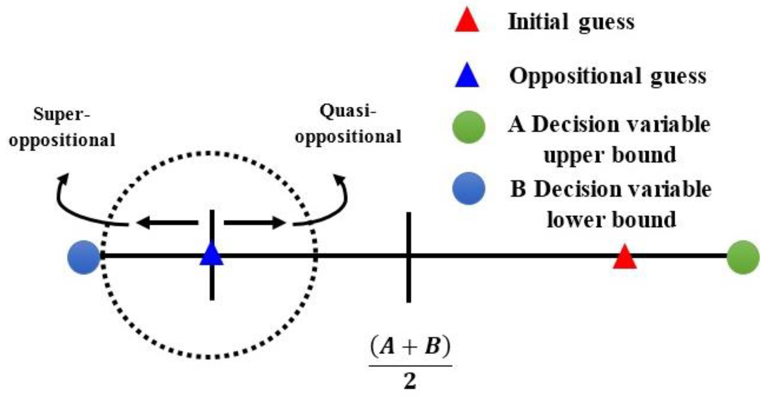
3.1. Oppositional-Based Learning (OL)
3.2. The UPSO
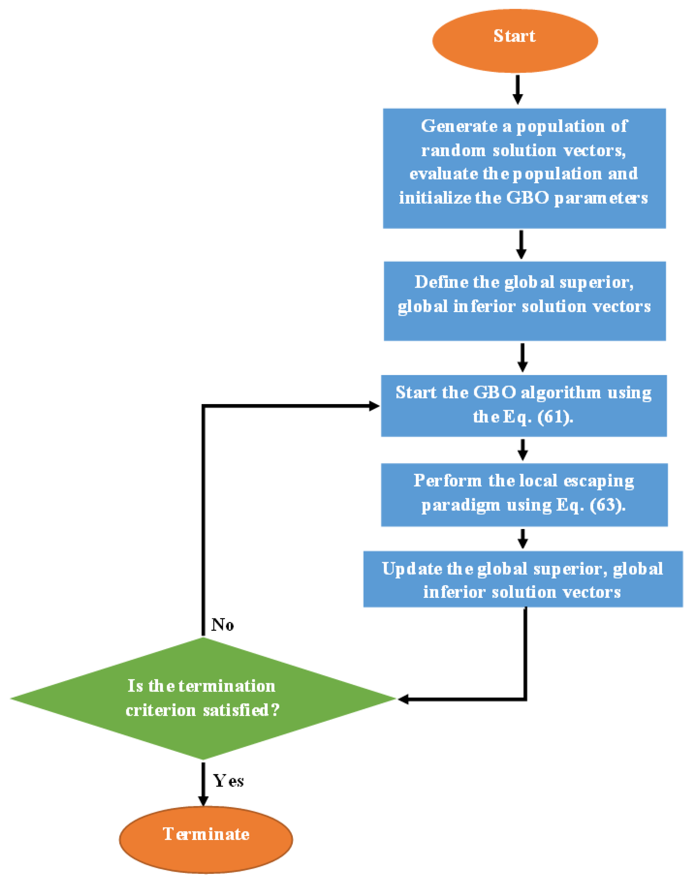
3.3. The GBO Algorithm
3.3.1. The Initialization Stage
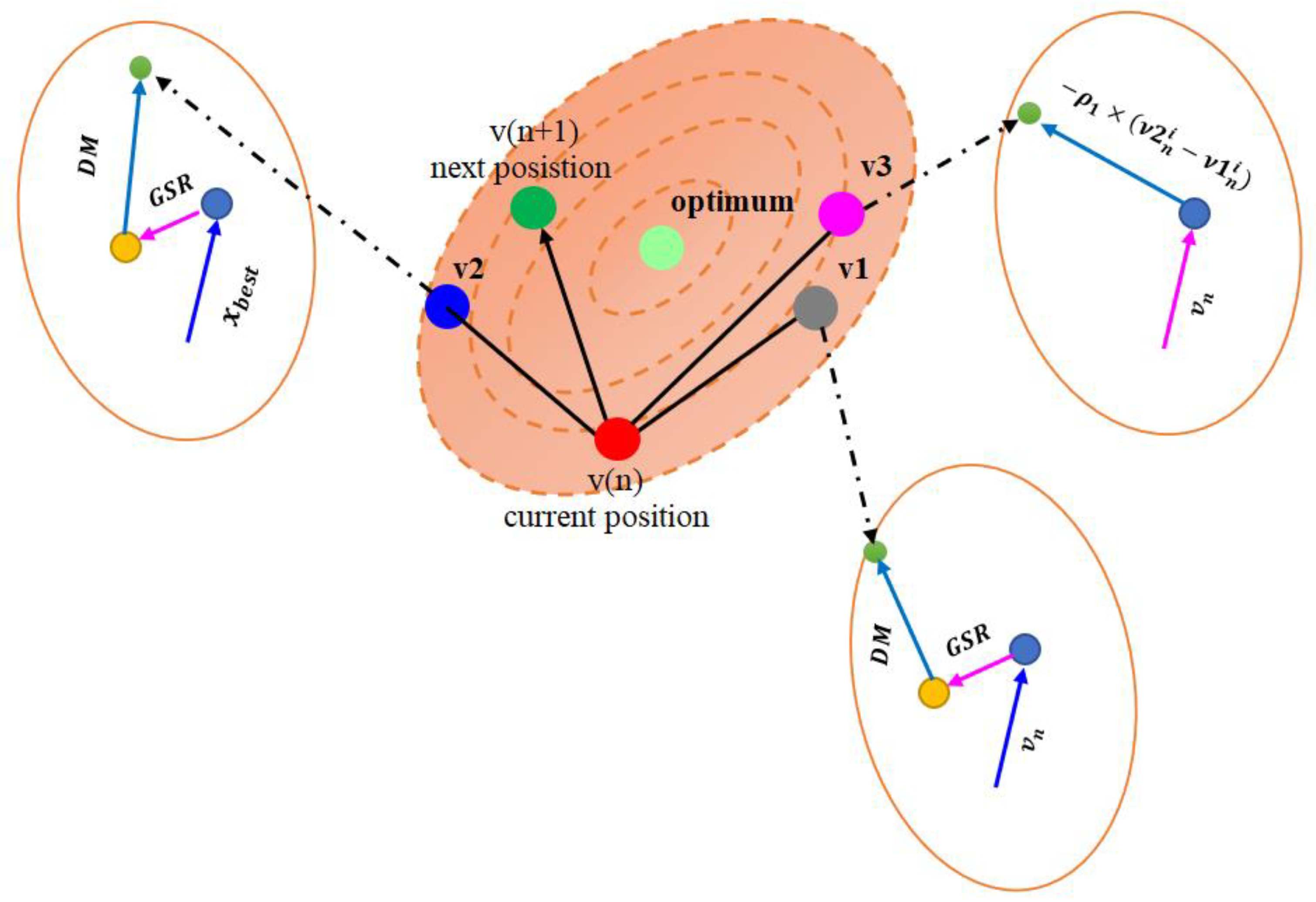
3.3.2. The GSR Stage
3.3.3. The Local Escaping Stage
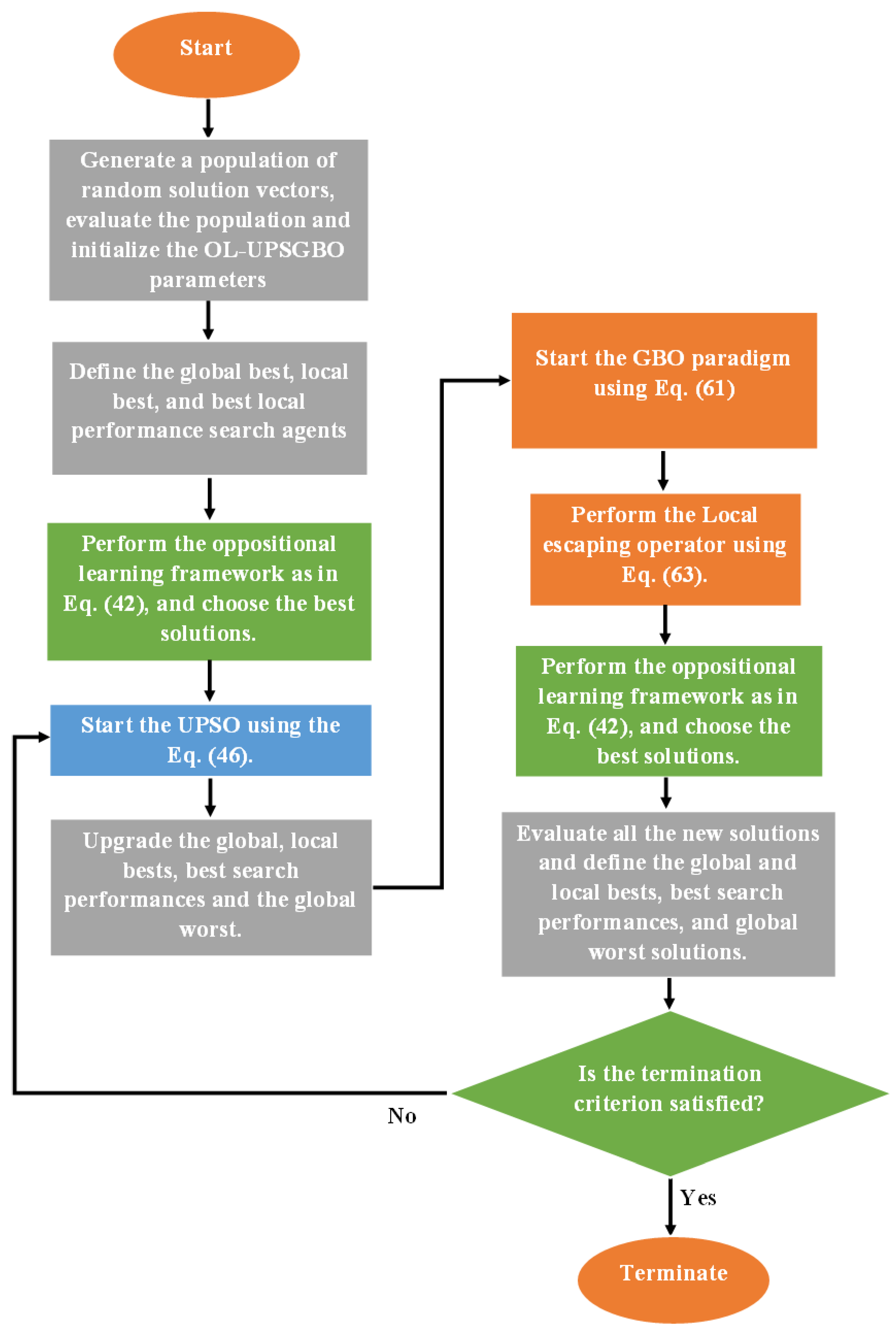
3.4. The Proposed OL-UPSGBO Algorithm
3.5. Benchmarking of the OL-UPSGBO Algorithm
4. Inverse Analysis of Structural Damage Using the Developed Approach
- A.
- Initialization stage
- 1.
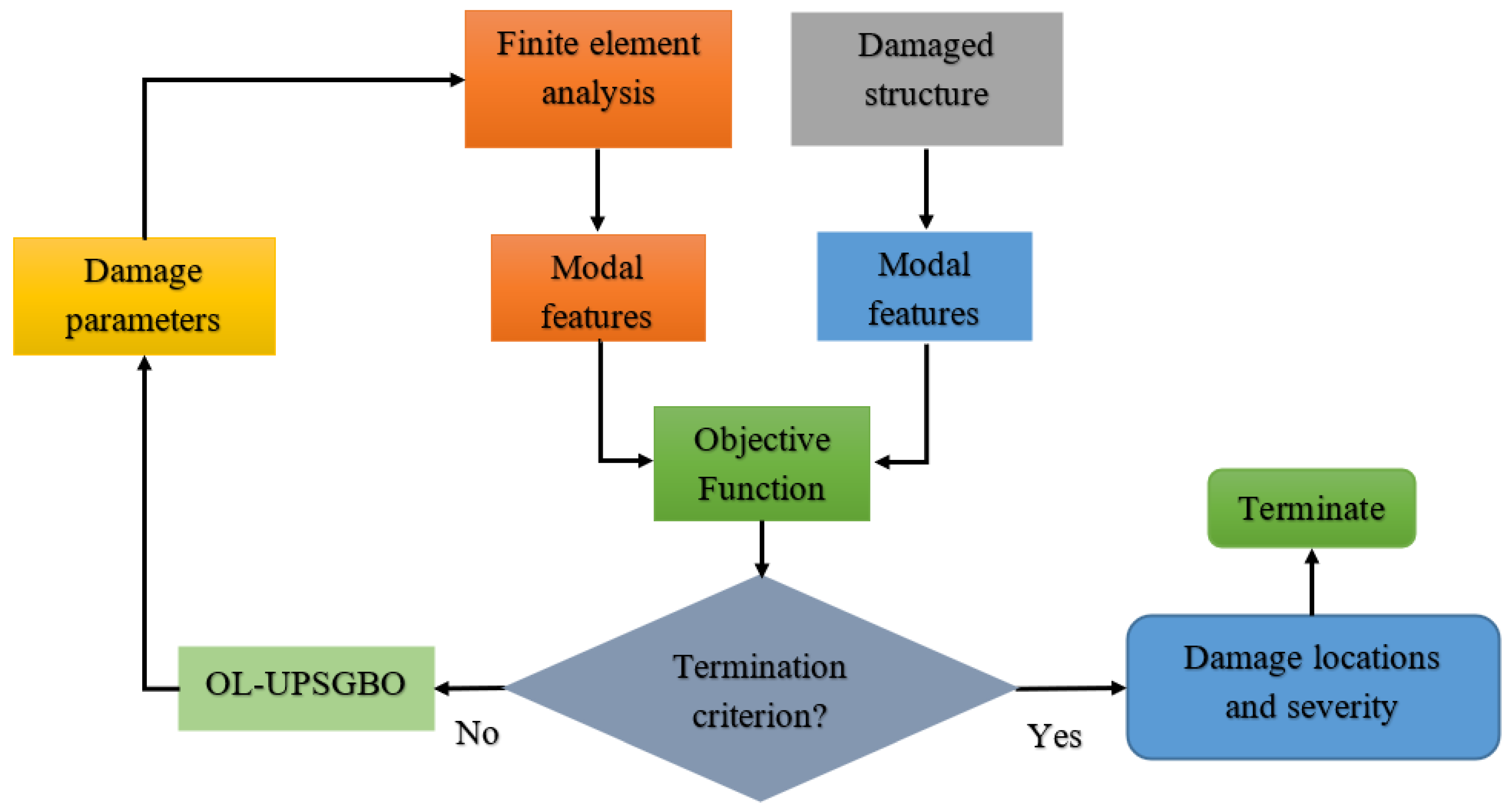
- Develop the FE model of the structure using a commercial software or a self-coded model.
- 2.
- Set a population of search agents, which are the damage indicators related to the overall structural or substructural elements, where each search agent represents one configuration of the FE model of the structure.
- 3.
- Extract the modal features related to the intact and damaged structure, and calculate the MSEn-, MKEn-, and mode shape-based sub-objectives using Equations (37)–(39). Thereafter, calculate the objective function using Equation (40) for each corresponding FE model configuration related to each candidate search agent.
- 4.
- Evaluate all the search agents using the developed objective function (as in Equation (40)).
- 5.
- Initialize all the stochastic parameters of the OL-UPSOGBO algorithm, as in Table 1.
- 6.
- Define the initial best global and local solutions, worst global solution, and the best performance of each search agent.
- 7.
- Apply the OL paradigm as in Equation (42).
- B.
- Iterative stage
- 1.
- Start the UPSO framework by calculating the global and local velocities as in Equation (45).
- 2.
- Update the population using Equation (46).
- 3.
- Update the best global and local solutions, worst global solution, and the best performance of each search agent.
- 4.
- Start the GBO stage by employing Equation (61).
- 5.
- Apply the local escaping operator, as in Equation (63).
- 6.
- Apply the OL paradigm, as in Equation (42).
- 7.
- Update the best global and local solutions, worst global solution, and the best performance of each search agent.
- 8.
- Break if termination criteria are satisfied.
- C.
- Damage identification stage
- 1.
- After termination of the iterative process, the best performed search agent is selected and registered.
- 2.
- The best solution contains the damage parameters corresponding to each element .
- 3.
- Elicit the damage locations and calculate the damage severities using Equation (41), and analyze the results.
5. Conclusions
Author Contributions
Funding
Institutional Review Board Statement
Informed Consent Statement
Data Availability Statement
Conflicts of Interest
References
- Toh, G.; Park, J. Review of vibration-based structural health monitoring using deep learning. Appl. Sci. 2020, 10, 1680. [Google Scholar] [CrossRef]
- Moughty, J.J.; Casas, J.R. A state of the art review of modal-based damage detection in bridges: Development, challenges and solutions. Appl. Sci. 2017, 7, 510. [Google Scholar] [CrossRef] [Green Version]
- Dolati, S.S.K.; Caluk, N.; Mehrabi, A.; Dolati, S.S.K. Non-destructive testing applications for steel bridges. Appl. Sci. 2021, 11, 9757. [Google Scholar] [CrossRef]
- Caicedo, D.; Lara-Valencia, L.; Valencia, Y. Machine learning techniques and population-based metaheuristics for damage detection and localization through frequency and modal-based structural health monitoring: A review. Arch. Comput. Methods Eng. 2022, 29, 3541–3565. [Google Scholar] [CrossRef]
- Alkayem, N.F.; Cao, M.; Zhang, Y.; Bayat, M.; Su, Z. Structural damage detection using finite element model updating with evolutionary algorithms: A survey. Neural Comput. Appl. 2018, 30, 389–411. [Google Scholar] [CrossRef] [PubMed] [Green Version]
- Minh, H.-L.; Sang-To, T.; Wahab, M.A.; Cuong-Le, T. Structural damage identification in thin-shell structures using a new technique combining finite element model updating and improved Cuckoo search algorithm. Adv. Eng. Softw. 2022, 173, 103206. [Google Scholar] [CrossRef]
- Minh, H.-L.; Sang-To, T.; Wahab, M.A.; Cuong-Le, T. A new metaheuristic optimization based on K-means clustering algorithm and its application to structural damage identification. Knowl.-Based Syst. 2022, 251, 109189. [Google Scholar] [CrossRef]
- Ereiz, S.; Duvnjak, I.; Jiménez-Alonso, J.F. Review of finite element model updating methods for structural applications. Structures 2022, 41, 684–723. [Google Scholar] [CrossRef]
- Lu, Z.; Lv, Y.; Ouyang, H. A super-harmonic feature based updating method for crack identification in rotors using a kriging surrogate model. Appl. Sci. 2019, 9, 2428. [Google Scholar] [CrossRef] [Green Version]
- Ereiz, S.; Duvnjak, I.; Jiménez-Alonso, J.F. Structural finite element model updating optimization based on game theory. Mater. Today Proc. 2022, 65, 1425–1432. [Google Scholar] [CrossRef]
- Ding, Z.; Hou, R.; Xia, Y. Structural damage identification considering uncertainties based on a Jaya algorithm with a local pattern search strategy and L0.5 sparse regularization. Eng. Struct. 2022, 261, 114312. [Google Scholar] [CrossRef]
- Ding, Z.; Li, J.; Hao, H. Simultaneous identification of structural damage and nonlinear hysteresis parameters by an evolutionary algorithm-based artificial neural network. Int. J. Non-Linear Mech. 2022, 142, 103970. [Google Scholar] [CrossRef]
- Al-Hababi, T.; Al-Kayem, N.F.; Cui, L.; Zhang, S.; Liu, C.; Cao, M. The coupled effect of temperature changes and damage depth on natural frequencies in beam-like structures. Struct. Durab. Health Monit. 2022, 16, 15–35. [Google Scholar] [CrossRef]
- Al-Hababi, T.; Cao, M.; Al-Kayem, N.F.; Shi, B.; Wei, Q.; Cui, L.; Šumarac, D.; Ragulskis, M. The dual Fourier transform spectra (DFTS): A new nonlinear damage indicator for identification of breathing cracks in beam-like structures. Nonlinear Dyn. 2022, 1–23. [Google Scholar] [CrossRef]
- Al-Hababi, T.; Al-Kayem, N.F.; Zhu, H.; Cui, L.; Zhang, S.; Cao, M. Effective identification and localization of single and multiple breathing cracks in beams under gaussian excitation using time-domain analysis. Mathematics 2022, 10, 1853. [Google Scholar] [CrossRef]
- Al-Hababi, T.; Cao, M.; Saleh, B.; Alkayem, N.F.; Xu, H. A critical review of nonlinear damping identification in structural dynamics: Methods, applications, and challenges. Sensors 2020, 20, 7303. [Google Scholar] [CrossRef]
- Yang, X.; Ouyang, H.; Guo, X.; Cao, S. Modal strain energy-based model updating method for damage identification on beam-like structures. J. Struct. Eng. 2020, 146, 04020246. [Google Scholar] [CrossRef]
- Wang, N.; Zhu, R.-H.; Wang, Q.-M.; Zheng, J.-H.; Zhang, J.-B. A method for quantitative damage identification in a high-piled wharf based on modal strain energy residual variability. Ocean Eng. 2022, 254, 111314. [Google Scholar] [CrossRef]
- Moradipour, P.; Chan, T.H.; Gallage, C. Benchmark studies for bridge health monitoring using an improved modal strain energy method. Procedia Eng. 2017, 188, 194–200. [Google Scholar] [CrossRef]
- Yan, W.-J.; Ren, W.-X. A direct algebraic method to calculate the sensitivity of element modal strain energy. Int. J. Numer. Methods Biomed. Eng. 2011, 27, 694–710. [Google Scholar] [CrossRef]
- Entezami, A.; Shariatmadar, H. Damage detection in structural systems by improved sensitivity of modal strain energy and Tikhonov regularization method. Int. J. Dyn. Control 2014, 2, 509–520. [Google Scholar] [CrossRef] [Green Version]
- Vo-Duy, T.; Ho-Huu, V.; Dang-Trung, H.; Nguyen-Thoi, T. A two-step approach for damage detection in laminated composite structures using modal strain energy method and an improved differential evolution algorithm. Compos. Struct. 2016, 147, 42–53. [Google Scholar] [CrossRef]
- Dinh-Cong, D.; Nguyen-Thoi, T.; Nguyen, D.T. A two-stage multi-damage detection approach for composite structures using MKECR-Tikhonov regularization iterative method and model updating procedure. Appl. Math. Model. 2021, 90, 114–130. [Google Scholar] [CrossRef]
- Dinh-Cong, D.; Nguyen-Thoi, T.; Vinyas, M.; Nguyen, D.T. Two-stage structural damage assessment by combining modal kinetic energy change with symbiotic organisms search. Int. J. Struct. Stab. Dyn. 2019, 19, 1950120. [Google Scholar] [CrossRef]
- Joseph, J.T.; Chan, T.H.T.; Nguyen, K.-D. Correlation-based damage identification and quantification using modal kinetic energy change. Int. J. Struct. Stab. Dyn. 2020, 20, 2042007. [Google Scholar] [CrossRef]
- Joseph, J.T.; Chan, T.H.T.; Nguyen, A.; Nguyen, K.D. Damage identification of civil structures using modal kinetic energy change approach. In ACMSM25. Lecture Notes in Civil Engineering; Wang, C., Ho, J., Kitipornchai, S., Eds.; Springer: Singapore, 2020; Volume 37. [Google Scholar]
- Pooya, S.M.H.; Massumi, A. A novel damage detection method in beam-like structures based on the relation between modal kinetic energy and modal strain energy and using only damaged structure data. J. Sound Vib. 2022, 530, 116943. [Google Scholar] [CrossRef]
- Torkzadeh, P.; Goodarzi, Y.; Salajegheh, E. A two-stage damage detection method for large-scale structures by kinetic and modal strain energies using heuristic particle swarm optimization. Int. J. Optim. Civ. Eng. 2013, 3, 465–482. [Google Scholar]
- Xu, M.; Wang, S.; Jiang, Y. Structural damage identification by a cross modal energy sensitivity based mode subset selection strategy. Mar. Struct. 2021, 77, 102968. [Google Scholar] [CrossRef]
- Shahri, A.H.; Ghorbani-Tanha, A. Damage detection via closed-form sensitivity matrix of modal kinetic energy change ratio. J. Sound Vib. 2017, 401, 268–281. [Google Scholar] [CrossRef]
- Gomes, G.F.; Mendez, Y.A.D.; da Silva Lopes Alexandrino, P.; da Cunha, S.S.; Ancelotti, A.C. A review of vibration based inverse methods for damage detection and identification in mechanical structures using optimization algorithms and ANN. Arch. Comput. Methods Eng. 2019, 26, 883–897. [Google Scholar] [CrossRef]
- Jafarkhani, R.; Masri, S.F. Finite element model updating using evolutionary strategy for damage detection. Comput.-Aided Civ. Infrastruct. Eng. 2011, 26, 207–224. [Google Scholar] [CrossRef]
- Kaveh, A.; Hosseini, S.M.; Zaerreza, A. A physics-based metaheuristic algorithm based on Doppler effect phenomenon and mean euclidian distance threshold. Period. Polytech. Civ. Eng. 2022, 66, 820–842. [Google Scholar] [CrossRef]
- Wang, G.-G.; Deb, S.; Coelho, L.d.S. Elephant herding optimization. In Proceedings of the 3rd International Symposium on Computational and Business Intelligence (ISCBI), Bali, Indonesia, 7–9 December 2015. [Google Scholar]
- Wang, G.-G. Moth search algorithm: A bio-inspired metaheuristic algorithm for global optimization problems. Memetic Comput. 2018, 10, 151–164. [Google Scholar] [CrossRef]
- Parsopoulos, K.E.; Vrahatis, M.N. Unified particle swarm optimization for solving constrained engineering optimization problems. In Advances in Natural Computation. ICNC 2005. Lecture Notes in Computer Science; Wang, L., Chen, K., Ong, Y.S., Eds.; Springer: Berlin/Heidelberg, Germany, 2005; Volume 3612. [Google Scholar]
- Ghannadi, P.; Kourehli, S.S. Efficiency of the slime mold algorithm for damage detection of large-scale structures. Struct. Des. Tall Spec. Build. 2022, e1967. [Google Scholar] [CrossRef]
- Ghannadi, P.; Kourehli, S.S.; Noori, M.; Altabey, W.A. Efficiency of grey wolf optimization algorithm for damage detection of skeletal structures via expanded mode shapes. Adv. Struct. Eng. 2020, 23, 2850–2865. [Google Scholar] [CrossRef]
- Ghannadi, P.; Kourehli, S.S. Multiverse optimizer for structural damage detection: Numerical study and experimental validation. Struct. Des. Tall Spec. Build. 2020, 29, e1777. [Google Scholar] [CrossRef]
- Gomes, G.F.; Giovani, R.S. An efficient two-step damage identification method using sunflower optimization algorithm and mode shape curvature (MSDBI–SFO). Eng. Comput. 2020, 38, 1711–1730. [Google Scholar] [CrossRef]
- Pereira, J.L.J.; Francisco, M.B.; Jr, S.S.d.C.; Gomes, G.F. A powerful Lichtenberg optimization algorithm: A damage identification case study. Eng. Appl. Artif. Intell. 2021, 97, 104055. [Google Scholar] [CrossRef]
- Pereira, J.L.J.; Chuman, M.; Jr, S.S.C.; Gomes, G.F. Lichtenberg optimization algorithm applied to crack tip identification in thin plate-like structures. Eng. Comput. 2021, 38, 151–166. [Google Scholar] [CrossRef]
- Khatir, S.; Tiachacht, S.; Thanh, C.L.; Tran-Ngoc, H.; Mirjalili, S.; Wahab, M.A. A robust FRF damage indicator combined with optimization techniques for damage assessment in complex truss structures. Case Stud. Constr. Mater. 2022, 17, e01197. [Google Scholar] [CrossRef]
- Tran-Ngoc, H.; Khatir, S.; Le-Xuan, T.; Tran-Viet, H.; Bui-Tien, T.; De Roeck, G.; Wahab, M. A. Damage assessment in structures using artificial neural network working and a hybrid stochastic optimization. Sci. Rep. 2022, 12, 1–12. [Google Scholar] [CrossRef] [PubMed]
- Minh, H.-L.; Khatir, S.; Rao, R.V.; Wahab, M.A.; Cuong-Le, T. A variable velocity strategy particle swarm optimization algorithm (VVS-PSO) for damage assessment in structures. Eng.Comput. 2021. [Google Scholar] [CrossRef]
- To, T.S.; Le, M.H.; Danh, T.T.; Khatir, S.; Abdel Wahab, M.; Le, T.C. Combination of intermittent search strategy and an Improve Particle Swarm Optimization algorithm (IPSO) for model updating. Frat. Ed Integrità Strutt. 2022, 59, 141–152. [Google Scholar]
- Kaveh, A.; Akbari, H.; Hosseini, S.M. Plasma generation optimization: A new physically-based metaheuristic algorithm for solving constrained optimization problems. Eng. Comput. 2020, 38, 1554–1606. [Google Scholar] [CrossRef]
- Kaveh, A.; Vaez, S.R.H.; Hosseini, P.; Fallah, N. Detection of damage in truss structures using Simplified Dolphin Echolocation algorithm based on modal data. Smart Struct. Syst. 2016, 18, 983–1004. [Google Scholar] [CrossRef]
- Kaveh, A.; Hosseini, S.M.; Zaerreza, A. boundary strategy for optimization-based structural damage detection problem using metaheuristic algorithms. Period. Polytech. Civ. Eng. 2020, 65, 150–167. [Google Scholar] [CrossRef]
- Mohebian, P.; Aval, S.B.B.; Noori, M.; Lu, N.; Altabey, W.A. Visible particle series search algorithm and its application in structural damage identification. Sensors 2022, 22, 1275. [Google Scholar] [CrossRef]
- Aval, S.B.B.; Mohebian, P. Joint damage identification in frame structures by integrating a new damage index with equilibrium optimizer algorithm. Int. J. Struct. Stab. Dyn. 2022, 22, 2250056. [Google Scholar] [CrossRef]
- Aval, S.B.B.; Mohebian, P. A novel optimization algorithm based on modal force information for structural damage identification. Int. J. Struct. Stab. Dyn. 2021, 21, 2150100. [Google Scholar] [CrossRef]
- Ahmadianfar, I.; Bozorg-Haddad, O.; Chu, X. Gradient-based optimizer: A new metaheuristic optimization algorithm. Inf. Sci. 2020, 540, 131–159. [Google Scholar] [CrossRef]
- Li, J.; Gao, Y.; Zhang, H.; Yang, Q. Self-adaptive opposition-based differential evolution with subpopulation strategy for numerical and engineering optimization problems. Complex Intell. Syst. 2022, 8, 2051–2089. [Google Scholar] [CrossRef]
- Wang, W.-C.; Xu, L.; Chau, K.-W.; Zhao, Y.; Xu, D.-M. An orthogonal opposition-based-learning Yin–Yang-pair optimization algorithm for engineering optimization. Eng. Comput. 2021, 38, 1149–1183. [Google Scholar] [CrossRef]
- Clerc, M.; Kennedy, J. The particle swarm-explosion, stability and convergence in a multidimensional complex space. IEEE Trans. Evol. Comput. 2002, 6, 58–73. [Google Scholar] [CrossRef] [Green Version]
- Tsai, H.C. Unified particle swarm delivers high efficiency to particle swarm optimization. Appl. Soft Comput. 2017, 55, 371–383. [Google Scholar] [CrossRef]
- Wu, G.; Mallipeddi, R.; Suganthan, P.N. Problem Definitions and Evaluation Criteria for the CEC 2017 Competition and Special Session on Constrained Single Objective Real-Parameter Optimization; Technical Report; National University of Defense Technology: Changsha, China; Kyungpook National University: Daegu, Republic of Korea; Nanyang Technological University: Singapore, 20 September 2017. [Google Scholar]
- Suganthan, P.N. Available online: https://github.com/P-N-Suganthan/2020-RW-Constrained-Optimisation (accessed on 15 July 2022).
- Mirjalili, S.; Mirjalili, S.M.; Lewis, A. Grey wolf optimizer. Adv. Eng. Softw. 2014, 69, 46–61. [Google Scholar] [CrossRef] [Green Version]
- Mirjalili, S.; Lewis, A. The whale optimization algorithm. Adv. Eng. Softw. 2016, 95, 51–67. [Google Scholar] [CrossRef]
- Mirjalili, S.; Mirjalili, S.M.; Hatamlou, A. Multi-verse optimizer: A nature-inspired algorithm for global optimization. Neural Comput. Appl. 2016, 27, 495–513. [Google Scholar] [CrossRef]
- Mirjalili, S. SCA: A Sine Cosine Algorithm for solving optimization problems. Knowl.-Based Syst. 2016, 96, 120–133. [Google Scholar] [CrossRef]
- Abualigah, L.; Diabat, A.; Mirjalili, S.; Elaziz, M.; Gandomi, A.H. The arithmetic optimization algorithm. Comput. Methods Appl. Mech. Eng. 2021, 376, 113609. [Google Scholar] [CrossRef]
- Faramarzi, A.; Heidarinejad, M.; Stephens, B.; Mirjalili, S. Equilibrium optimizer: A novel optimization algorithm☆. Knowl.-Based Syst. 2020, 191, 105190. [Google Scholar] [CrossRef]
- Abualigah, L.; Yousri, D.; Elaziz, M.A.; Ewees, A.A.; Al-Qanesse, M.A.A.; Gandomi, A.H. Aquila Optimizer: A novel meta-heuristic optimization algorithm. Comput. Ind. Eng. 2021, 157, 107250. [Google Scholar] [CrossRef]
- Johnson, E.A.; Lam, H.F.; Katafygiotis, L.S.; Beck, J.L. Phase II of the ASCE benchmark study on SHM. In Proceedings of the 15th ASCE Engineering Mechanics Conference, New York, NY, USA, 2–5 June 2002. [Google Scholar]
- Johnson, E.A.; Lam, H.F.; Katafygiotis, L.S.; Beck, J.L. Phase I IASC-ASCE structural health monitoring benchmark problem using simulated data. J. Eng. Mech. 2004, 130, 3–15. [Google Scholar] [CrossRef]


| Function Type | No. | Function | Optimum |
|---|---|---|---|
| Unimodal | Shifted and Rotated Bent Cigar Function | 100 | |
| NA | NA | ||
| Shifted and Rotated Zakharov Function | 300 | ||
| Multimodal | Shifted and Rotated Rosenbrock’s Function | 400 | |
| Shifted and Rotated Rastrigin’s Function | 500 | ||
| Shifted and Rotated Expanded Scaffer’s Function | 600 | ||
| Shifted and Rotated Lunacek Bi_Rastrigin Function | 700 | ||
| Shifted and Rotated Non-Continuous Rastrigin’s Function | 800 | ||
| Shifted and Rotated Levy Function | 900 | ||
| Shifted and Rotated Schwefel’s Function | 1000 | ||
| Hybrid | Hybrid Function 1 (N = 3) | 1100 | |
| Hybrid Function 2 (N = 3) | 1200 | ||
| Hybrid Function 3 (N = 3) | 1300 | ||
| Hybrid Function 4 (N = 4) | 1400 | ||
| Hybrid Function 5 (N = 4) | 1500 | ||
| Hybrid Function 6 (N = 4) | 1600 | ||
| Hybrid Function 6 (N = 5) | 1700 | ||
| Hybrid Function 6 (N = 5) | 1800 | ||
| Hybrid Function 6 (N = 5) | 1900 | ||
| Hybrid Function 6 (N = 6) | 2000 | ||
| Composite | Composition Function 1 (N = 3) | 2100 | |
| Composition Function 2 (N = 3) | 2200 | ||
| Composition Function 3 (N = 4) | 2300 | ||
| Composition Function 4 (N = 4) | 2400 | ||
| Composition Function 5 (N = 5) | 2500 | ||
| Composition Function 6 (N = 5) | 2600 | ||
| Composition Function 7 (N = 6) | 2700 | ||
| Composition Function 8 (N = 6) | 2800 | ||
| Composition Function 9 (N = 3) | 2900 | ||
| Composition Function 10 (N = 3) | 3000 |
| Algorithm | Parameters |
|---|---|
| GWO | Default stochastic parameter descending from 2 to 0. |
| WOA | Default stochastic parameter one descending from 2 to 0. Default stochastic parameter two descending from 2 to 0. |
| SCA | Default stochastic parameter descending from 2 to 0. |
| MVO | Traveling distance rate (default) Wormhole existence probability (default) |
| AOA | Default stochastic parameters: MOP_Max = 1; MOP_Min = 0.2; Alpha = 5; Mu = 0.499; |
| EO | Default stochastic parameters: a1 = 5; a2 = 1; GP = 0.5; |
| AO | Default stochastic parameters: alpha = 0.1; delta = 0.1; |
| OL-UPSGBO | (default) (default) (default) |
| Function | Property | GWO | WOA | MVO | SCA | GBO | AOA | EO | AO | OLPSGBO |
|---|---|---|---|---|---|---|---|---|---|---|
| Ave | 1.1 × 10⁹ | 2.6 × 10⁶ | 3.7 × 10⁸ | 1.6 × 10¹⁰ | 1.9 × 10³ | 2.0 × 10⁸ | 5.6 × 10³ | 3.0 × 10² | 1.5 × 10² | |
| Min | 5.5 × 10⁸ | 7.2 × 10⁵ | 2.8 × 10⁸ | 1.0 × 10¹⁰ | 3.2 × 10² | 9.4 × 10³ | 1.2 × 10² | 1.1 × 10² | 1.0 × 10² | |
| Max | 2.7 × 10⁹ | 5.3 × 10⁶ | 4.2 × 10⁸ | 2.1 × 10¹⁰ | 5.1 × 10³ | 8.2 × 10⁸ | 1.7 × 10⁴ | 9.2 × 10² | 2.9 × 10² | |
| STD | 6.5 × 10⁸ | 1.2 × 10⁶ | 4.5 × 10⁷ | 2.8 × 10⁹ | 1.9 × 10³ | 3.0 × 10⁸ | 5.3 × 10³ | 2.5 × 10² | 7.4 × 101 | |
| Rank | 8 | 5 | 7 | 9 | 3 | 6 | 4 | 2 | 1 | |
| NA | NA | NA | NA | NA | NA | NA | NA | NA | NA | |
| Ave | 2.9 × 10⁴ | 2.0 × 10⁵ | 1.8 × 10³ | 4.5 × 10⁴ | 3.0 × 10² | 7.8 × 10⁴ | 7.3 × 10² | 3.0 × 10⁴ | 3.0 × 10² | |
| Min | 8.3 × 10³ | 9.9 × 10⁴ | 1.6 × 10³ | 4.0 × 10⁴ | 3.0 × 10² | 6.0 × 10⁴ | 4.0 × 10² | 2.1 × 10⁴ | 3.0 × 10² | |
| Max | 3.9 × 10⁴ | 3.5 × 10⁵ | 2.0 × 10³ | 5.6 × 10⁴ | 3.0 × 10² | 8.8 × 10⁴ | 1.4 × 10³ | 3.5 × 10⁴ | 3.0 × 10² | |
| STD | 9.0 × 10³ | 7.6 × 10⁴ | 1.4 × 10² | 5.3 × 10⁴ | 2.3 × 10⁻² | 9.5 × 10³ | 3.3 × 10² | 4.9 × 10³ | 1.3 × 10⁻³ | |
| Rank | 8 | 5 | 7 | 9 | 3 | 6 | 4 | 2 | 1 | |
| Ave | 5.8 × 10² | 5.6 × 10² | 5.2 × 10² | 1.6 × 10³ | 4.5 × 10² | 1.0 × 10⁴ | 5.0 × 10² | 5.5 × 10² | 4.0 × 10² | |
| Min | 5.4 × 10² | 4.8 × 10² | 5.0 × 10² | 1.2 × 10³ | 4.0 × 10² | 5.6 × 10³ | 4.7 × 10² | 5.2 × 10² | 4.0 × 10² | |
| Max | 6.3 × 10² | 6.5 × 10² | 5.3 × 10² | 2.3 × 10³ | 4.8 × 10² | 1.3 × 10⁴ | 5.2 × 10² | 6.1 × 10² | 4.0 × 10² | |
| STD | 3.4 × 101 | 4.6 × 101 | 1.2 × 101 | 3.5 × 10² | 3.1 × 101 | 2.6 × 10³ | 1.6 × 101 | 2.9 × 101 | 2.1 × 10² | |
| Rank | 8 | 5 | 7 | 9 | 3 | 6 | 4 | 2 | 1 | |
| Ave | 5.7 × 10² | 7.9 × 10² | 7.0 × 10² | 8.0 × 10² | 6.7 × 10² | 8.2 × 10² | 5.6 × 10² | 6.7 × 10² | 6.3 × 10² | |
| Min | 5.6 × 10² | 7.1 × 10² | 6.7 × 10² | 7.7 × 10² | 6.2 × 10² | 7.5 × 10² | 5.3 × 10² | 6.4 × 10² | 5.8 × 10² | |
| Max | 6.0 × 10² | 9.5 × 10² | 7.3 × 10² | 8.2 × 10² | 7.1 × 10² | 8.6 × 10² | 6.0 × 10² | 7.0 × 10² | 6.6 × 10² | |
| STD | 1.4 × 101 | 7.1 × 101 | 2.1 × 101 | 1.7 × 101 | 2.4 × 101 | 3.4 × 101 | 2.0 × 101 | 2.0 × 101 | 2.9 × 101 | |
| Rank | 2 | 7 | 6 | 8 | 5 | 9 | 1 | 4 | 3 | |
| Ave | 6.1 × 10² | 6.7 × 10² | 6.2 × 10² | 6.6 × 10² | 6.2 × 10² | 6.7 × 10² | 6.0 × 10² | 6.5 × 10² | 6.1 × 10² | |
| Min | 6.1 × 10² | 6.6 × 10² | 6.1 × 10² | 6.5 × 10² | 6.1 × 10² | 6.5 × 10² | 6.0 × 10² | 6.4 × 10² | 6.0 × 10² | |
| Max | 6.2 × 10² | 6.8 × 10² | 6.3 × 10² | 6.7 × 10² | 6.2 × 10² | 6.7 × 10² | 6.0 × 10² | 6.5 × 10² | 6.2 × 10² | |
| STD | 2.0 × 101 | 7.1 × 101 | 7.3 × 101 | 6.0 × 101 | 4.9 × 101 | 6.4 × 101 | 8.0 × 10⁻² | 5.4 × 101 | 6.0 × 101 | |
| Rank | 3 | 9 | 4 | 7 | 5 | 8 | 1 | 6 | 2 | |
| Ave | 9.3 × 10² | 1.3 × 10³ | 9.8 × 10² | 1.1 × 10³ | 9.3 × 10² | 1.3 × 10³ | 8.0 × 10² | 1.0 × 10³ | 8.8 × 10² | |
| Min | 9.1 × 10² | 1.1 × 10³ | 9.4 × 10² | 1.1 × 10³ | 8.9 × 10² | 1.2 × 10³ | 7.6 × 10² | 9.4 × 10² | 8.2 × 10² | |
| Max | 9.6 × 10² | 1.5 × 10³ | 1.0 × 10² | 1.2 × 10³ | 9.8 × 10² | 1.4 × 10³ | 8.3 × 10² | 1.1 × 10³ | 9.2 × 10² | |
| STD | 1.6 × 101 | 1.1 × 10² | 2.4 × 101 | 2.4 × 101 | 3.3 × 101 | 4.8 × 101 | 2.0 × 101 | 5.1 × 101 | 3.0 × 101 | |
| Rank | 4 | 8 | 5 | 7 | 3 | 9 | 1 | 6 | 2 | |
| Ave | 9.4 × 10² | 1.0 × 10³ | 1.0 × 10³ | 1.1 × 10³ | 9.3 × 10² | 1.1 × 10³ | 8.7 × 10² | 9.3 × 10² | 9.1 × 10² | |
| Min | 9.1 × 10² | 9.6 × 10² | 9.7 × 10² | 1.0 × 10³ | 8.9 × 10² | 1.0 × 10³ | 8.4 × 10² | 8.9 × 10² | 8.8 × 10² | |
| Max | 9.6 × 10² | 1.1 × 10³ | 1.1 × 10³ | 1.1 × 10³ | 9.8 × 10² | 1.1 × 10³ | 9.0 × 10² | 9.6 × 10² | 9.3 × 10² | |
| STD | 1.4 × 101 | 6.3 × 101 | 4.0 × 101 | 1.6 × 101 | 3.3 × 101 | 3.4 × 101 | 1.9 × 101 | 2.3 × 101 | 1.8 × 101 | |
| Rank | 5 | 6 | 7 | 9 | 4 | 8 | 1 | 3 | 2 | |
| Ave | 1.7 × 10³ | 7.5 × 10³ | 1.3 × 10³ | 5.6 × 10³ | 2.0 × 10³ | 5.8 × 10³ | 9.0 × 10² | 5.2 × 10³ | 1.6 × 10³ | |
| Min | 1.2 × 10³ | 5.1 × 10³ | 1.0 × 10³ | 4.4 × 10³ | 1.4 × 10³ | 4.5 × 10³ | 9.0 × 10² | 3.5 × 10³ | 1.2 × 10³ | |
| Max | 2.4 × 10³ | 1.0 × 10⁴ | 2.5 × 10³ | 6.5 × 10³ | 3.3 × 10³ | 7.2 × 10³ | 9.1 × 10² | 7.1 × 10³ | 2.1 × 10³ | |
| STD | 3.5 × 10² | 1.8 × 10³ | 4.7 × 10² | 6.8 × 10² | 6.2 × 10² | 8.0 × 10² | 4.5 × 101 | 1.1 × 10³ | 3.1 × 10² | |
| Rank | 5 | 6 | 7 | 9 | 4 | 8 | 1 | 3 | 2 | |
| Ave | 5.9 × 10³ | 6.4 × 10³ | 7.2 × 10³ | 8.2 × 10³ | 5.1 × 10³ | 6.8 × 10³ | 4.6 × 10³ | 4.9 × 10³ | 4.5 × 10³ | |
| Min | 4.7 × 10³ | 5.3 × 10³ | 6.6 × 10³ | 7.4 × 10³ | 4.5 × 10³ | 6.0 × 10³ | 3.3 × 10³ | 4.0 × 10³ | 3.8 × 10³ | |
| Max | 6.5 × 10³ | 8.4 × 10³ | 8.1 × 10³ | 8.7 × 10³ | 7.0 × 10³ | 7.7 × 10³ | 5.8 × 10³ | 5.7 × 10³ | 5.2 × 10³ | |
| STD | 5.4 × 10² | 1.0 × 10³ | 4.8 × 10² | 4.0 × 10² | 7.5 × 10² | 5.7 × 10² | 8.6 × 10² | 5.4 × 10² | 4.1 × 10² | |
| Rank | 5 | 6 | 7 | 9 | 4 | 8 | 1 | 3 | 2 | |
| Ave | 1.5 × 10³ | 1.5 × 10³ | 1.4 × 10³ | 2.4 × 10³ | 1.2 × 10³ | 4.4 × 10³ | 1.4 × 10³ | 1.4 × 10³ | 1.2 × 10³ | |
| Min | 1.3 × 10³ | 1.3 × 10³ | 1.3 × 10³ | 2.0 × 10³ | 1.2 × 10³ | 1.8 × 10³ | 1.3 × 10³ | 1.3 × 10³ | 1.2 × 10³ | |
| Max | 2.1 × 10³ | 1.7 × 10³ | 1.5 × 10³ | 2.9 × 10³ | 1.3 × 10³ | 8.6 × 10³ | 1.4 × 10³ | 1.5 × 10³ | 1.2 × 10³ | |
| STD | 2.7 × 10² | 1.5 × 10² | 4.9 × 101 | 3.3 × 10² | 2.7 × 101 | 2.3 × 10³ | 6.5 × 101 | 6.3 × 101 | 1.1 × 101 | |
| Rank | 7 | 6 | 5 | 8 | 2 | 9 | 3 | 4 | 1 | |
| Ave | 9.6 × 10⁷ | 4.1 × 10⁷ | 4.7 × 10⁷ | 1.5 × 10⁹ | 2.9 × 10⁴ | 9.2 × 10⁹ | 7.5 × 10⁵ | 1.5 × 10⁷ | 2.9 × 10⁴ | |
| Min | 5.5 × 10⁷ | 9.3 × 10⁶ | 3.4 × 10⁷ | 7.6 × 10⁸ | 1.3 × 10⁴ | 4.0 × 10⁹ | 3.0 × 10⁵ | 3.0 × 10⁶ | 1.3 × 10⁴ | |
| Max | 1.8 × 10⁸ | 1.4 × 10⁸ | 7.0 × 10⁷ | 2.2 × 10⁹ | 4.2 × 10⁴ | 1.2 × 10¹⁰ | 2.0 × 10⁶ | 2.6 × 10⁷ | 4.3 × 10⁴ | |
| STD | 4.1 × 10⁷ | 3.8 × 10⁷ | 1.2 × 10⁷ | 5.0 × 10⁸ | 1.0 × 10⁴ | 2.6 × 10⁹ | 5.1 × 10⁵ | 6.9 × 10⁶ | 1.1 × 10⁴ | |
| Rank | 7 | 6 | 5 | 8 | 2 | 9 | 3 | 4 | 1 | |
| Ave | 2.5 × 10⁷ | 1.1 × 10⁵ | 1.7 × 10⁷ | 6.4 × 10⁸ | 1.0 × 10⁴ | 9.3 × 10⁷ | 4.3 × 10⁴ | 3.2 × 10⁵ | 7.6 × 10³ | |
| Min | 1.2 × 10⁷ | 4.3 × 10⁴ | 8.0 × 10⁶ | 3.8 × 10⁸ | 3.0 × 10³ | 2.4 × 10⁴ | 9.4 × 10³ | 7.6 × 10⁴ | 2.5 × 10³ | |
| Max | 5.2 × 10⁷ | 2.5 × 10⁵ | 2.1 × 10⁷ | 9.5 × 10⁸ | 1.8 × 10⁴ | 6.1 × 10⁸ | 1.0 × 10⁵ | 5.4 × 10⁵ | 1.5 × 10⁴ | |
| STD | 1.2 × 10⁷ | 6.4 × 10⁴ | 5.0 × 10⁶ | 2.0 × 10⁸ | 6.3 × 10³ | 1.9 × 10⁸ | 2.8 × 10⁴ | 1.3 × 10⁵ | 4.5 × 10³ | |
| Rank | 7 | 4 | 6 | 9 | 2 | 8 | 3 | 5 | 1 | |
| Ave | 8.0 × 10⁴ | 4.7 × 10⁵ | 1.9 × 10⁴ | 2.1 × 10⁵ | 1.8 × 10³ | 7.1 × 10⁴ | 6.2 × 10⁴ | 2.9 × 10⁵ | 1.7 × 10³ | |
| Min | 1.6 × 10⁴ | 1.6 × 10⁴ | 4.2 × 10³ | 4.6 × 10⁴ | 1.6 × 10³ | 1.7 × 10⁴ | 2.4 × 10⁴ | 3.7 × 10⁴ | 1.6 × 10³ | |
| Max | 2.5 × 10⁵ | 2.0 × 10⁶ | 3.2 × 10⁴ | 5.6 × 10⁵ | 3.2 × 10³ | 1.4 × 10⁵ | 1.0 × 10⁵ | 8.3 × 10⁵ | 1.7 × 10³ | |
| STD | 7.0 × 10⁴ | 6.1 × 10⁵ | 7.9 × 10³ | 1.9 × 10⁵ | 5.0 × 10² | 3.9 × 10⁴ | 2.6 × 10⁴ | 2.3 × 10⁵ | 4.9 × 101 | |
| Rank | 6 | 9 | 3 | 7 | 2 | 5 | 4 | 8 | 1 | |
| Ave | 4.9 × 10⁵ | 9.5 × 10⁴ | 1.8 × 10⁶ | 2.0 × 10⁷ | 1.2 × 10⁴ | 2.1 × 10⁴ | 2.3 × 10⁴ | 7.6 × 10⁴ | 2.5 × 10³ | |
| Min | 1.4 × 10⁵ | 1.7 × 10⁴ | 9.3 × 10⁵ | 1.9 × 10⁶ | 1.9 × 10³ | 1.6 × 10⁴ | 7.5 × 10³ | 3.1 × 10⁴ | 1.6 × 10³ | |
| Max | 1.1 × 10⁶ | 1.9 × 10⁵ | 2.6 × 10⁶ | 4.4 × 10⁷ | 4.0 × 10⁴ | 4.4 × 10⁴ | 5.9 × 10⁴ | 1.5 × 10⁵ | 5.3 × 10³ | |
| STD | 2.7 × 10⁵ | 5.0 × 10⁴ | 6.3 × 10⁵ | 1.2 × 10⁷ | 1.3 × 10⁴ | 8.9 × 10³ | 1.7 × 10⁴ | 3.8 × 10⁴ | 1.3 × 10³ | |
| Rank | 7 | 6 | 8 | 9 | 2 | 3 | 4 | 5 | 1 | |
| Ave | 2.6 × 10³ | 3.3 × 10³ | 2.9 × 10³ | 3.8 × 10³ | 2.7 × 10³ | 3.9 × 10³ | 2.6 × 10³ | 3.1 × 10³ | 2.4 × 10³ | |
| Min | 2.3 × 10³ | 2.5 × 10³ | 2.4 × 10³ | 3.5 × 10³ | 2.4 × 10³ | 3.0 × 10³ | 2.0 × 10³ | 2.6 × 10³ | 2.1 × 10³ | |
| Max | 2.8 × 10³ | 3.8 × 10³ | 3.3 × 10³ | 4.0 × 10³ | 3.1 × 10³ | 4.8 × 10³ | 3.2 × 10³ | 4.0 × 10³ | 2.6 × 10³ | |
| STD | 1.9 × 10² | 4.3 × 10² | 2.6 × 10² | 1.6 × 10² | 2.5 × 10² | 5.2 × 10² | 3.7 × 10² | 4.1 × 10² | 1.9 × 10² | |
| Rank | 3 | 7 | 5 | 8 | 4 | 9 | 2 | 6 | 1 | |
| Ave | 2.0 × 10³ | 2.5 × 10³ | 2.1 × 10³ | 2.5 × 10³ | 2.3 × 10³ | 2.7 × 10³ | 2.2 × 10³ | 2.3 × 10³ | 2.1 × 10³ | |
| Min | 1.9 × 10³ | 2.1 × 10³ | 2.0 × 10³ | 2.3 × 10³ | 2.0 × 10³ | 2.5 × 10³ | 2.0 × 10³ | 1.8 × 10³ | 1.9 × 10³ | |
| Max | 2.1 × 10³ | 2.9 × 10³ | 2.3 × 10³ | 2.7 × 10³ | 2.7 × 10³ | 3.2 × 10³ | 2.3 × 10³ | 2.6 × 10³ | 2.3 × 10³ | |
| STD | 7.7 × 101 | 2.4 × 10² | 1.0 × 10² | 1.7 × 10² | 2.5 × 10² | 2.6 × 10² | 9.6 × 101 | 2.4 × 10² | 1.6 × 10² | |
| Rank | 1 | 8 | 3 | 6 | 5 | 9 | 4 | 7 | 2 | |
| Ave | 1.3 × 10⁶ | 2.8 × 10⁶ | 3.3 × 10⁵ | 5.1 × 10⁶ | 3.3 × 10⁴ | 1.1 × 10⁶ | 4.0 × 10⁵ | 1.6 × 10⁶ | 1.7 × 10⁴ | |
| Min | 9.8 × 10⁴ | 2.7 × 10⁵ | 1.8 × 10⁵ | 2.8 × 10⁶ | 1.1 × 10⁴ | 1.6 × 10⁵ | 1.5 × 10⁵ | 2.2 × 10⁵ | 2.7 × 10³ | |
| Max | 7.2 × 10⁶ | 9.7 × 10⁶ | 4.6 × 10⁵ | 8.3 × 10⁶ | 9.4 × 10⁴ | 2.6 × 10⁶ | 7.7 × 10⁵ | 5.6 × 10⁶ | 3.3 × 10⁴ | |
| STD | 2.1 × 10⁶ | 3.1 × 10⁶ | 1.1 × 10⁵ | 1.7 × 10⁶ | 2.9 × 10⁴ | 6.7 × 10⁵ | 1.9 × 10⁵ | 2.0 × 10⁶ | 1.1 × 10⁴ | |
| Rank | 5 | 8 | 3 | 9 | 2 | 6 | 4 | 7 | 1 | |
| Ave | 1.5 × 10⁶ | 2.8 × 10⁶ | 2.4 × 10⁶ | 3.8 × 10⁷ | 6.4 × 10³ | 2.7 × 10³ | 3.2 × 10⁴ | 8.0 × 10⁵ | 2.3 × 10³ | |
| Min | 3.0 × 10⁵ | 2.9 × 10⁵ | 1.2 × 10⁶ | 1.1 × 10⁷ | 2.0 × 10³ | 2.5 × 10³ | 3.2 × 10³ | 8.7 × 10⁴ | 2.0 × 10³ | |
| Max | 4.5 × 10⁶ | 7.4 × 10⁶ | 6.2 × 10⁶ | 8.6 × 10⁷ | 2.3 × 10⁴ | 2.9 × 10³ | 6.6 × 10⁴ | 1.8 × 10⁶ | 3.0 × 10³ | |
| STD | 1.2 × 10⁶ | 2.2 × 10⁶ | 1.4 × 10⁶ | 2.4 × 10⁷ | 6.1 × 10³ | 1.3 × 10² | 2.5 × 10⁴ | 6.1 × 10⁵ | 2.6 × 10² | |
| Rank | 6 | 8 | 7 | 9 | 3 | 2 | 4 | 5 | 1 | |
| Ave | 2.4 × 10³ | 2.8 × 10³ | 2.5 × 10³ | 2.7 × 10³ | 2.4 × 10³ | 2.7 × 10³ | 2.4 × 10³ | 2.5 × 10³ | 2.3 × 10³ | |
| Min | 2.2 × 10³ | 2.4 × 10³ | 2.2 × 10³ | 2.5 × 10³ | 2.2 × 10³ | 2.5 × 10³ | 2.3 × 10³ | 2.2 × 10³ | 2.2 × 10³ | |
| Max | 2.7 × 10³ | 3.0 × 10³ | 2.9 × 10³ | 2.9 × 10³ | 2.5 × 10³ | 2.9 × 10³ | 2.8 × 10³ | 2.8 × 10³ | 2.5 × 10³ | |
| STD | 1.3 × 10² | 1.9 × 10² | 1.9 × 10² | 1.3 × 10² | 1.2 × 10² | 1.1 × 10² | 2.0 × 10² | 1.8 × 10² | 1.2 × 10² | |
| Rank | 3 | 9 | 6 | 8 | 2 | 7 | 4 | 5 | 1 | |
| Ave | 2.4 × 10³ | 2.5 × 10³ | 2.5 × 10³ | 2.6 × 10³ | 2.4 × 10³ | 2.6 × 10³ | 2.4 × 10³ | 2.5 × 10³ | 2.4 × 10³ | |
| Min | 2.4 × 10³ | 2.5 × 10³ | 2.4 × 10³ | 2.5 × 10³ | 2.4 × 10³ | 2.6 × 10³ | 2.4 × 10³ | 2.4 × 10³ | 2.4 × 10³ | |
| Max | 2.5 × 10³ | 2.7 × 10³ | 2.5 × 10³ | 2.6 × 10³ | 2.5 × 10³ | 2.6 × 10³ | 2.5 × 10³ | 2.5 × 10³ | 2.5 × 10³ | |
| STD | 2.7 × 101 | 6.3 × 101 | 2.7 × 101 | 1.6 × 101 | 3.0 × 101 | 2.7 × 101 | 4.0 × 101 | 3.9 × 101 | 4.1 × 101 | |
| Rank | 4 | 7 | 6 | 8 | 3 | 9 | 1 | 5 | 2 | |
| Ave | 4.3 × 10³ | 6.0 × 10³ | 6.8 × 10³ | 9.1 × 10³ | 3.2 × 10³ | 8.5 × 10³ | 6.1 × 10³ | 2.8 × 10³ | 2.3 × 10³ | |
| Min | 2.5 × 10³ | 2.3 × 10³ | 2.4 × 10³ | 4.0 × 10³ | 2.3 × 10³ | 6.7 × 10³ | 2.3 × 10³ | 2.3 × 10³ | 2.3 × 10³ | |
| Max | 7.5 × 10³ | 8.5 × 10³ | 9.7 × 10³ | 1.0 × 10⁴ | 8.0 × 10³ | 9.3 × 10³ | 7.9 × 10³ | 6.6 × 10³ | 2.3 × 10³ | |
| STD | 2.2 × 10³ | 2.5 × 10³ | 3.1 × 10³ | 1.8 × 10³ | 2.0 × 10³ | 7.3 × 10² | 2.1 × 10³ | 1.4 × 10³ | 3.0 × 101 | |
| Rank | 4 | 5 | 7 | 9 | 3 | 8 | 6 | 2 | 1 | |
| Ave | 2.8 × 10³ | 3.1 × 10³ | 2.9 × 10³ | 3.0 × 10³ | 2.8 × 10³ | 3.4 × 10³ | 2.9 × 10³ | 2.8 × 10³ | 2.8 × 10³ | |
| Min | 2.8 × 10³ | 2.9 × 10³ | 2.8 × 10³ | 2.9 × 10³ | 2.7 × 10³ | 3.3 × 10³ | 2.7 × 10³ | 2.8 × 10³ | 2.8 × 10³ | |
| Max | 2.9 × 10³ | 3.3 × 10³ | 3.0 × 10³ | 3.0 × 10³ | 2.8 × 10³ | 3.6 × 10³ | 4.0 × 10³ | 2.9 × 10³ | 2.8 × 10³ | |
| STD | 1.7 × 101 | 1.4 × 10³ | 4.9 × 101 | 3.4 × 101 | 2.8 × 101 | 8.4 × 101 | 3.9 × 10³ | 4.0 × 101 | 1.3 × 101 | |
| Rank | 3 | 8 | 5 | 7 | 2 | 9 | 6 | 4 | 1 | |
| Ave | 3.0 × 10³ | 3.2 × 10³ | 3.0 × 10³ | 3.2 × 10³ | 3.0 × 10³ | 3.7 × 10³ | 3.0 × 10³ | 3.1 × 10³ | 2.9 × 10³ | |
| Min | 3.0 × 10³ | 3.1 × 10³ | 3.0 × 10³ | 3.1 × 10³ | 2.9 × 10³ | 3.6 × 10³ | 2.9 × 10³ | 2.9 × 10³ | 2.9 × 10³ | |
| Max | 3.0 × 10³ | 3.5 × 10³ | 3.0 × 10³ | 3.2 × 10³ | 3.0 × 10³ | 4.0 × 10³ | 3.9 × 10³ | 3.3 × 10³ | 3.0 × 10³ | |
| STD | 8.4 × 101 | 1.5 × 10² | 2.4 × 101 | 3.4 × 101 | 2.7 × 101 | 1.4 × 10² | 3.2 × 10² | 9.9 × 101 | 3.2 × 101 | |
| Rank | 4 | 7 | 3 | 8 | 2 | 9 | 5 | 6 | 1 | |
| Ave | 3.0 × 10³ | 2.9 × 10³ | 2.9 × 10³ | 3.2 × 10³ | 2.9 × 10³ | 4.5 × 10³ | 2.9 × 10³ | 2.9 × 10³ | 2.9 × 10³ | |
| Min | 2.9 × 10³ | 2.9 × 10³ | 2.9 × 10³ | 3.1 × 10³ | 2.9 × 10³ | 4.1 × 10³ | 2.9 × 10³ | 2.9 × 10³ | 2.9 × 10³ | |
| Max | 3.0 × 10³ | 2.9 × 10³ | 2.9 × 10³ | 3.3 × 10³ | 2.9 × 10³ | 5.4 × 10³ | 2.9 × 10³ | 2.9 × 10³ | 2.9 × 10³ | |
| STD | 3.0 × 101 | 1.5 × 101 | 1.0 × 101 | 6.0 × 101 | 9.8 × 101 | 3.8 × 10² | 1.5 × 101 | 1.8 × 101 | 9.0 × 101 | |
| Rank | 7 | 6 | 5 | 8 | 3 | 9 | 2 | 4 | 1 | |
| Ave | 5.4 × 10³ | 7.8 × 10³ | 5.2 × 10³ | 6.8 × 10³ | 4.8 × 10³ | 9.5 × 10³ | 4.9 × 10³ | 3.7 × 10³ | 4.6 × 10³ | |
| Min | 5.0 × 10³ | 6.2 × 10³ | 3.0 × 10³ | 5.0 × 10³ | 2.8 × 10³ | 8.0 × 10³ | 4.0 × 10³ | 2.9 × 10³ | 2.8 × 10³ | |
| Max | 5.7 × 10³ | 8.8 × 10³ | 6.0 × 10³ | 7.7 × 10³ | 5.7 × 10³ | 1.1 × 1004 | 6.2 × 10³ | 5.3 × 10³ | 5.8 × 10³ | |
| STD | 2.0 × 10² | 9.2 × 10² | 1.1 × 10³ | 7.4 × 10² | 1.0 × 10³ | 7.7 × 10² | 7.3 × 10² | 7.5 × 10² | 1.3 × 10³ | |
| Rank | 6 | 8 | 5 | 7 | 3 | 9 | 4 | 1 | 2 | |
| Ave | 3.3 × 10³ | 3.3 × 10³ | 3.2 × 10³ | 3.4 × 10³ | 3.2 × 10³ | 4.2 × 10³ | 3.2 × 10³ | 3.3 × 10³ | 3.2 × 10³ | |
| Min | 3.2 × 10³ | 3.3 × 10³ | 3.2 × 10³ | 3.3 × 10³ | 3.2 × 10³ | 3.9 × 10³ | 3.2 × 10³ | 3.2 × 10³ | 3.2 × 10³ | |
| Max | 3.3 × 10³ | 3.5 × 10³ | 3.2 × 10³ | 3.4 × 10³ | 3.3 × 10³ | 4.6 × 10³ | 3.3 × 10³ | 3.3 × 10³ | 3.3 × 10³ | |
| STD | 1.7 × 101 | 7.6 × 101 | 1.0 × 101 | 2.6 × 101 | 2.2 × 101 | 2.2 × 10² | 2.2 × 101 | 2.6 × 101 | 1.6 × 101 | |
| Rank | 5 | 7 | 1 | 8 | 4 | 9 | 3 | 6 | 2 | |
| Ave | 3.4 × 10³ | 3.3 × 10³ | 3.3 × 10³ | 4.0 × 10³ | 3.2 × 10³ | 6.3 × 10³ | 5.4 × 10³ | 3.3 × 10³ | 3.1 × 10³ | |
| Min | 3.3 × 10³ | 3.3 × 10³ | 3.2 × 10³ | 3.8 × 10³ | 3.1 × 10³ | 5.5 × 10³ | 3.2 × 10³ | 3.3 × 10³ | 3.1 × 10³ | |
| Max | 3.4 × 10³ | 3.3 × 10³ | 3.3 × 10³ | 4.3 × 10³ | 3.2 × 10³ | 7.5 × 10³ | 6.4 × 10³ | 3.4 × 10³ | 3.1 × 10³ | |
| STD | 3.3 × 101 | 1.8 × 101 | 2.1 × 101 | 1.6 × 10² | 6.1 × 101 | 6.7 × 10² | 1.5 × 10³ | 3.8 × 101 | 2.6 × 10⁻⁹ | |
| Rank | 6 | 3 | 5 | 7 | 2 | 9 | 8 | 4 | 1 | |
| Ave | 3.9 × 10³ | 5.0 × 10³ | 3.9 × 10³ | 4.7 × 10³ | 3.9 × 10³ | 6.3 × 10³ | 4.0 × 10³ | 4.3 × 10³ | 3.8 × 10³ | |
| Min | 3.6 × 10³ | 4.2 × 10³ | 3.7 × 10³ | 4.3 × 10³ | 3.6 × 10³ | 5.5 × 10³ | 3.8 × 10³ | 3.8 × 10³ | 3.5 × 10³ | |
| Max | 4.2 × 10³ | 5.9 × 10³ | 4.2 × 10³ | 5.1 × 10³ | 4.3 × 10³ | 7.5 × 10³ | 4.2 × 10³ | 4.8 × 10³ | 3.9 × 10³ | |
| STD | 1.6 × 10² | 5.2 × 10² | 1.6 × 10² | 2.1 × 10² | 2.2 × 10² | 6.7 × 10² | 1.4 × 10² | 3.7 × 10² | 1.4 × 10² | |
| Rank | 4 | 8 | 3 | 7 | 2 | 9 | 5 | 6 | 1 | |
| Ave | 8.0 × 10⁶ | 1.0 × 10⁷ | 4.1 × 10⁶ | 1.2 × 10⁸ | 7.7 × 10³ | 3.1 × 10⁷ | 1.4 × 10⁵ | 7.2 × 10⁶ | 6.1 × 10³ | |
| Min | 3.9 × 10⁶ | 1.6 × 10⁶ | 2.2 × 10⁶ | 6.1 × 10⁶ | 5.4 × 10³ | 5.3 × 10⁶ | 5.6 × 10³ | 3.4 × 10⁶ | 5.5 × 10³ | |
| Max | 1.3 × 10⁷ | 3.3 × 10⁷ | 9.6 × 10⁶ | 2.1 × 10⁸ | 1.4 × 10⁴ | 9.0 × 10⁷ | 7.3 × 10⁵ | 1.2 × 10⁷ | 6.5 × 10³ | |
| STD | 3.1 × 10⁶ | 8.9 × 10⁶ | 2.1 × 10⁶ | 5.2 × 10⁷ | 3.4 × 10³ | 2.4 × 10⁷ | 2.2 × 10⁵ | 2.9 × 10⁶ | 3.5 × 10² | |
| Rank | 6 | 7 | 4 | 9 | 2 | 8 | 3 | 5 | 1 | |
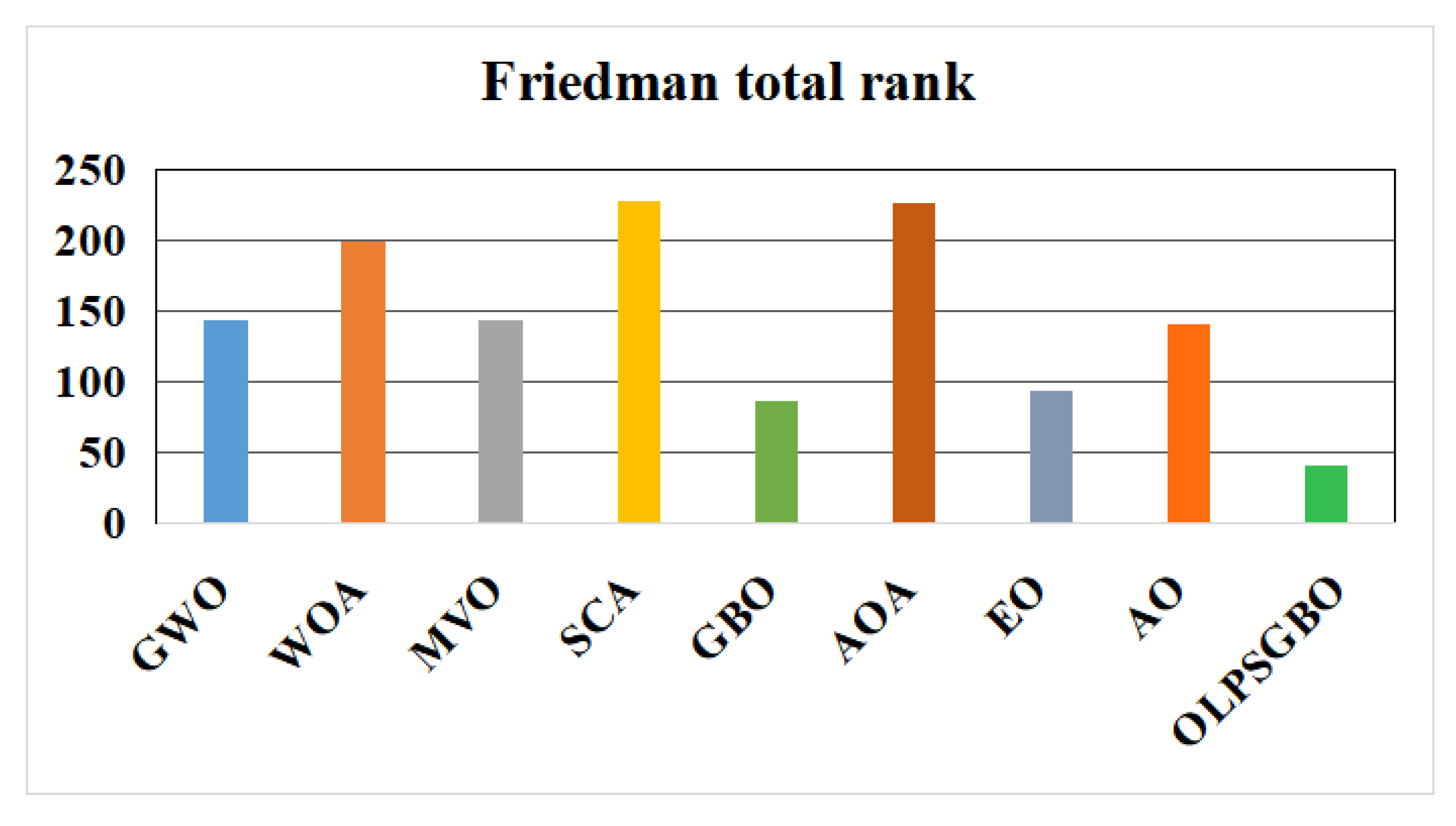
| Friedman average rank | 4.9655 | 6.8966 | 4.931 | 7.8621 | 2.9655 | 7.7931 | 3.2414 | 4.8276 | 1.3793 | |
| Friedman total rank | 144 | 200 | 143 | 228 | 86 | 226 | 94 | 140 | 40 | |
| Function | GWO | WOA | MVO | SCA | GBO | AOA | EO | AO |
|---|---|---|---|---|---|---|---|---|
| 0.001953125 | 0.001953125 | 0.001953125 | 0.001953125 | 0.001953125 | 0.001953125 | 0.001953125 | 0.193359375 | |
| NA | NA | NA | NA | NA | NA | NA | NA | |
| 0.001953125 | 0.001953125 | 0.001953125 | 0.001953125 | 0.001953125 | 0.001953125 | 0.001953125 | 0.001953125 | |
| 0.001953125 | 0.001953125 | 0.001953125 | 0.001953125 | 0.0078125 | 0.001953125 | 0.001953125 | 0.001953125 | |
| 0.001953125 | 0.001953125 | 0.001953125 | 0.001953125 | 0.03125 | 0.001953125 | 0.001953125 | 0.013671875 | |
| 0.275390625 | 0.001953125 | 0.064453125 | 0.001953125 | 0.01953125 | 0.001953125 | 0.001953125 | 0.001953125 | |
| 0.001953125 | 0.001953125 | 0.001953125 | 0.001953125 | 0.0078125 | 0.001953125 | 0.001953125 | 0.001953125 | |
| 0.01953125 | 0.001953125 | 0.001953125 | 0.001953125 | 0.193359375 | 0.001953125 | 0.00390625 | 0.232421875 | |
| 0.4921875 | 0.001953125 | 0.130859375 | 0.001953125 | 0.193359375 | 0.001953125 | 0.001953125 | 0.001953125 | |
| 0.001953125 | 0.001953125 | 0.001953125 | 0.001953125 | 0.048828125 | 0.001953125 | 0.921875 | 0.193359375 | |
| 0.001953125 | 0.001953125 | 0.001953125 | 0.001953125 | 0.625 | 0.001953125 | 0.001953125 | 0.001953125 | |
| 0.001953125 | 0.001953125 | 0.001953125 | 0.001953125 | 0.845703125 | 0.001953125 | 0.001953125 | 0.001953125 | |
| 0.001953125 | 0.001953125 | 0.001953125 | 0.001953125 | 0.556640625 | 0.001953125 | 0.00390625 | 0.001953125 | |
| 0.001953125 | 0.001953125 | 0.001953125 | 0.001953125 | 0.625 | 0.001953125 | 0.001953125 | 0.001953125 | |
| 0.001953125 | 0.001953125 | 0.001953125 | 0.001953125 | 0.001953125 | 0.001953125 | 0.001953125 | 0.001953125 | |
| 0.064453125 | 0.001953125 | 0.00390625 | 0.001953125 | 0.01953125 | 0.001953125 | 0.130859375 | 0.001953125 | |
| 0.064453125 | 0.013671875 | 0.845703125 | 0.009765625 | 0.275390625 | 0.001953125 | 0.625 | 0.01953125 | |
| 0.001953125 | 0.001953125 | 0.001953125 | 0.001953125 | 0.375 | 0.001953125 | 0.001953125 | 0.001953125 | |
| 0.001953125 | 0.001953125 | 0.001953125 | 0.001953125 | 0.009765625 | 0.013671875 | 0.001953125 | 0.001953125 | |
| 1 | 0.00390625 | 0.01953125 | 0.001953125 | 0.921875 | 0.001953125 | 0.6953125 | 0.064453125 | |
| 0.064453125 | 0.001953125 | 0.001953125 | 0.001953125 | 0.6953125 | 0.001953125 | 0.42578125 | 0.037109375 | |
| 0.001953125 | 0.001953125 | 0.001953125 | 0.001953125 | 0.6875 | 0.001953125 | 0.001953125 | 0.001953125 | |
| 0.001953125 | 0.001953125 | 0.001953125 | 0.001953125 | 0.4921875 | 0.001953125 | 0.6953125 | 0.009765625 | |
| 0.001953125 | 0.001953125 | 0.048828125 | 0.001953125 | 0.048828125 | 0.001953125 | 0.625 | 0.01953125 | |
| 0.001953125 | 0.00390625 | 0.009765625 | 0.001953125 | 0.275390625 | 0.001953125 | 0.921875 | 0.048828125 | |
| 0.02734375 | 0.001953125 | 0.083984375 | 0.00390625 | 0.845703125 | 0.001953125 | 0.921875 | 0.064453125 | |
| 0.048828125 | 0.001953125 | 0.375 | 0.001953125 | 0.4921875 | 0.001953125 | 0.556640625 | 0.00390625 | |
| 0.001953125 | 0.001953125 | 0.001953125 | 0.001953125 | 0.232421875 | 0.001953125 | 0.001953125 | 0.001953125 | |
| 0.037109375 | 0.001953125 | 0.16015625 | 0.001953125 | 0.375 | 0.001953125 | 0.048828125 | 0.005859375 | |
| 0.001953125 | 0.001953125 | 0.001953125 | 0.001953125 | 0.322265625 | 0.001953125 | 0.00390625 | 0.001953125 |
| Damage Scenario | Damage Locations | Damage Severity |
|---|---|---|
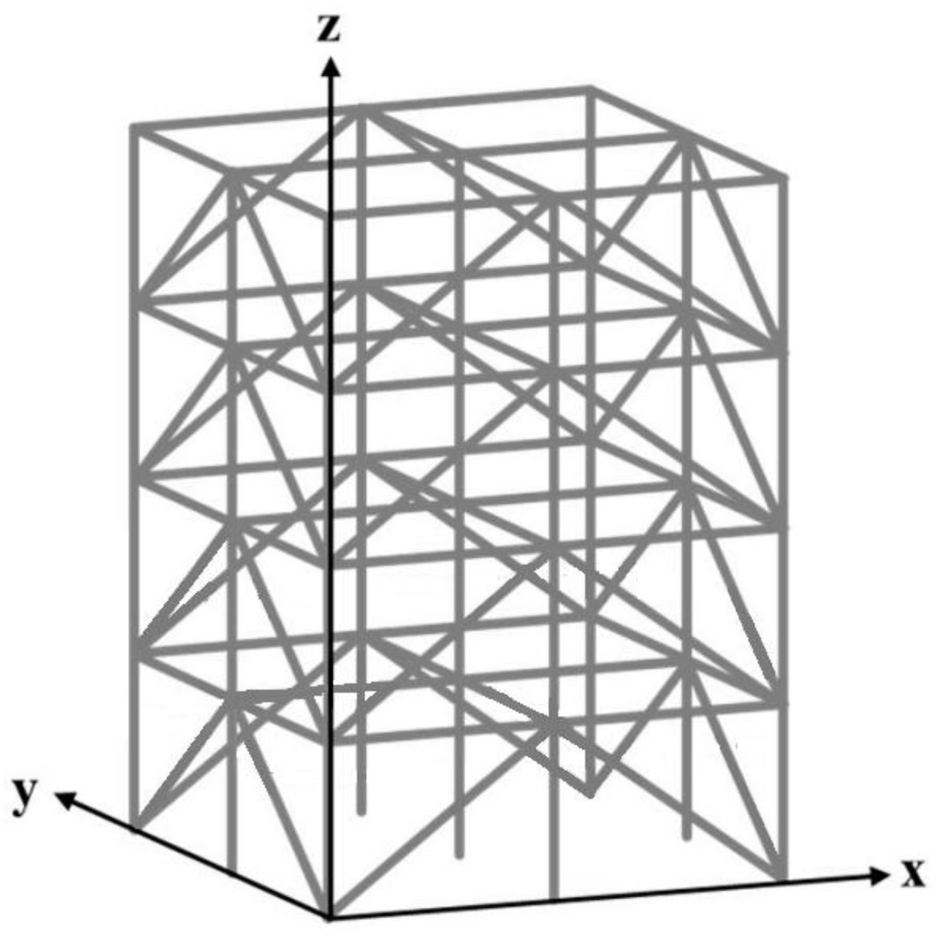
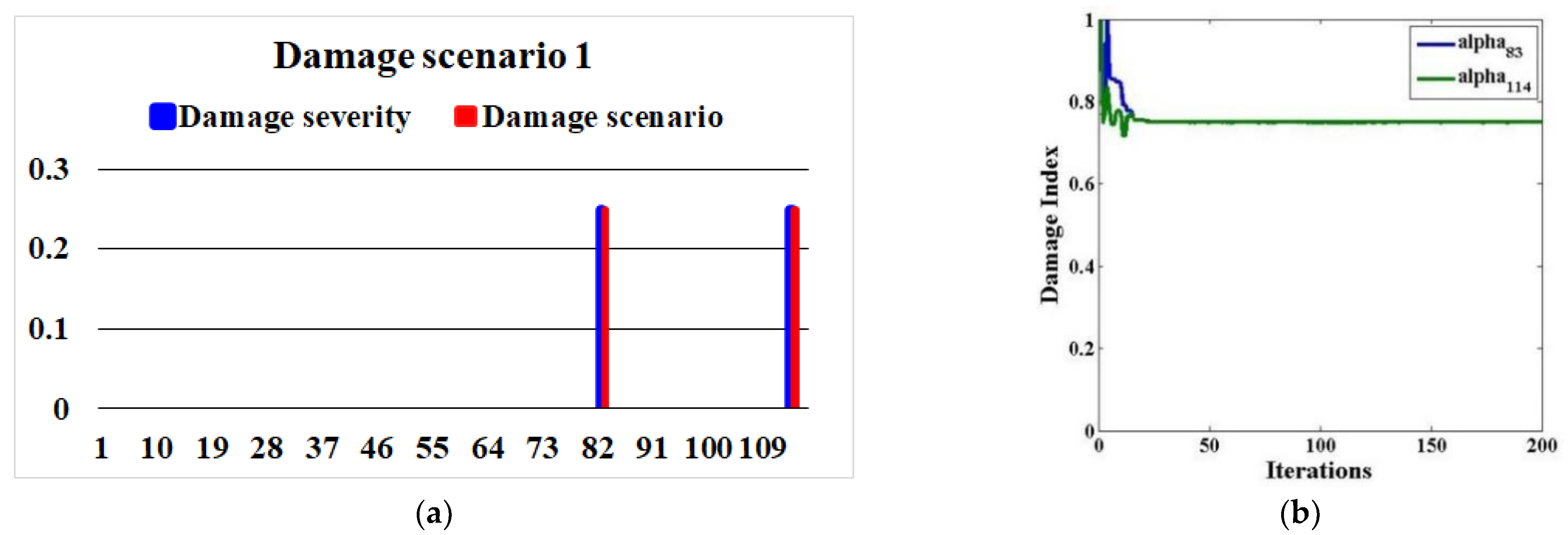
| Scenario 1 | Brace elements 83, and 114 | 25% |
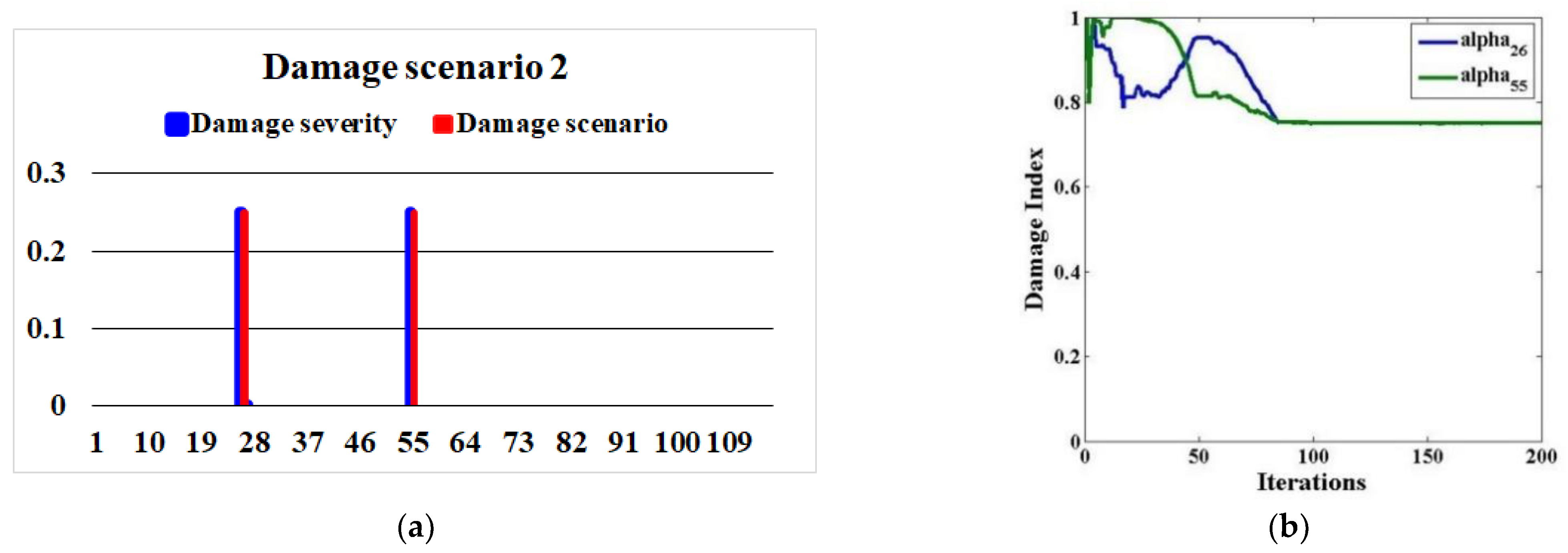
| Scenario 2 | Brace elements 26, and 55 | 25% |
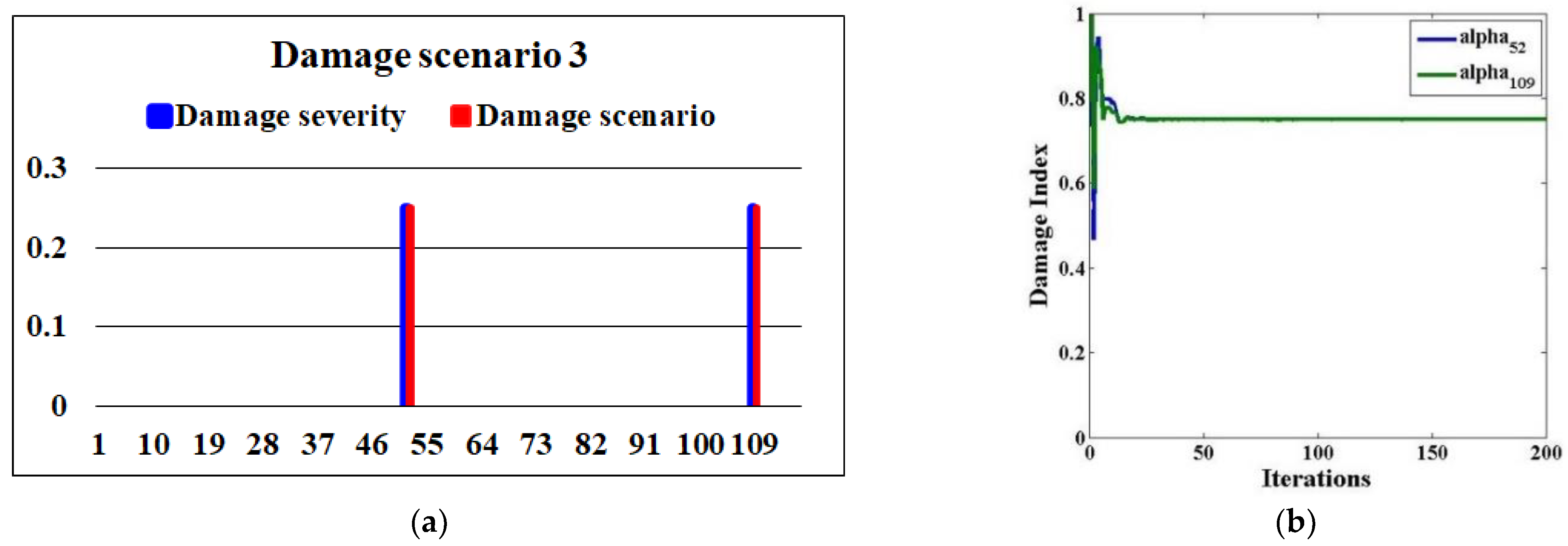
| Scenario 3 | Brace elements 52, and 109 | 25% |
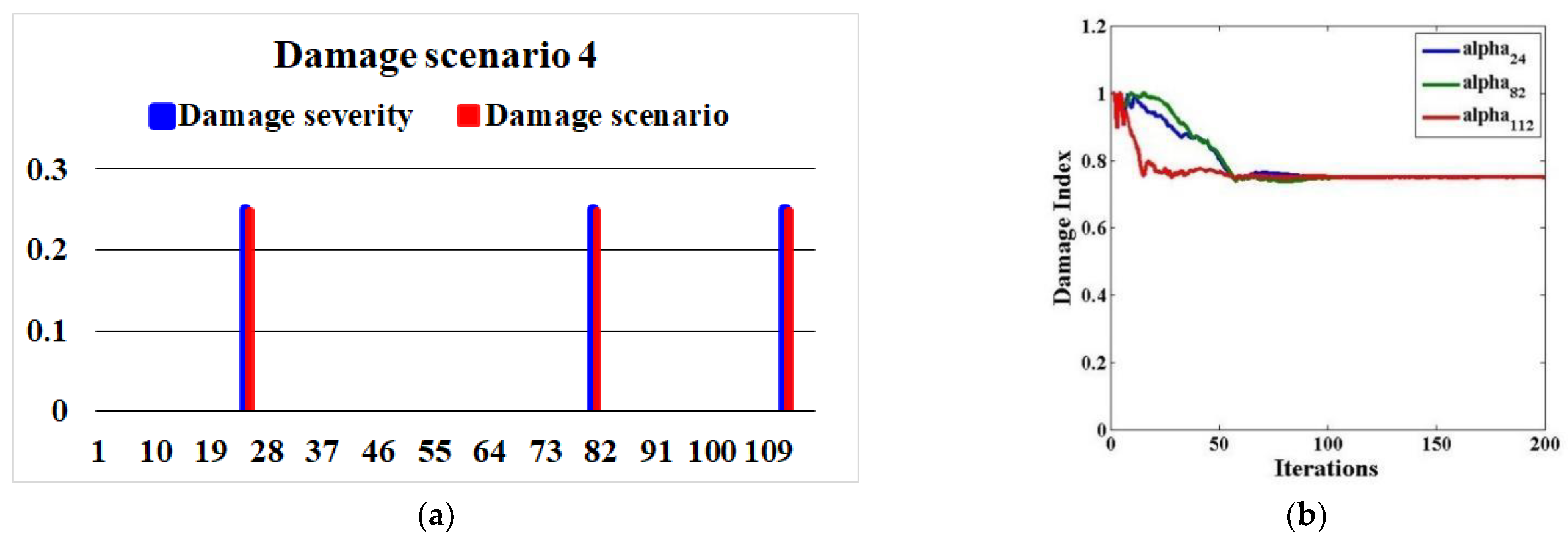
| Scenario 4 | Brace elements 24, 82, and 112 | 25% |
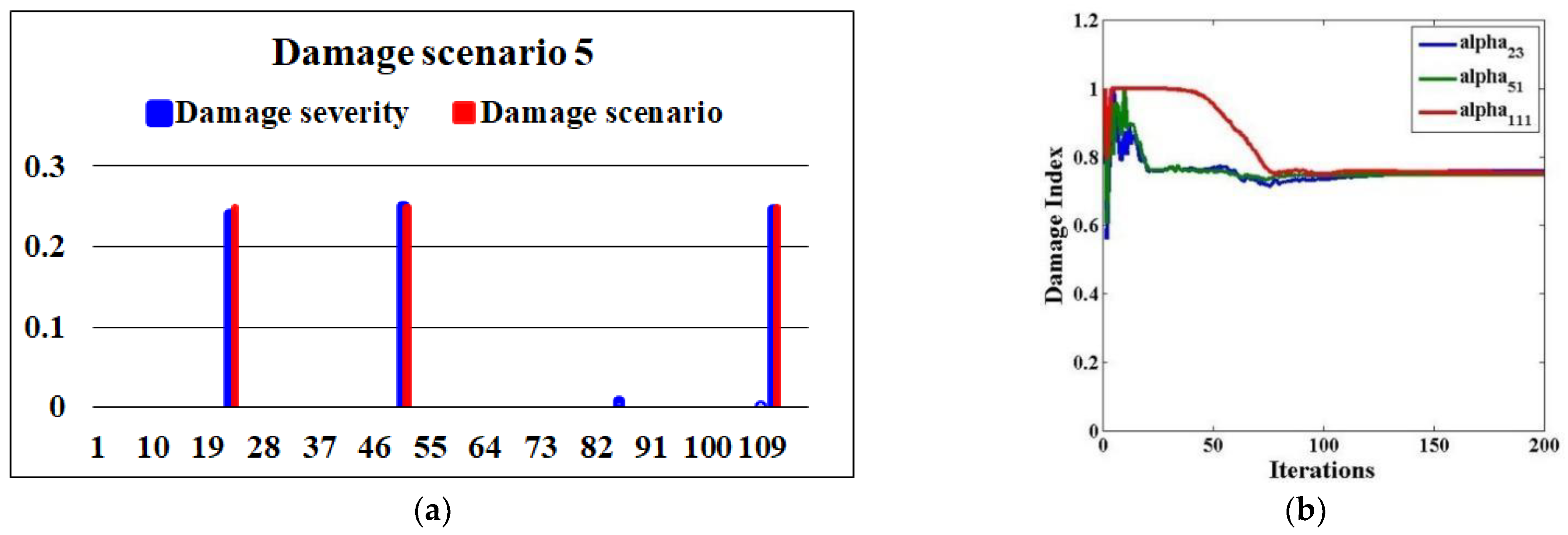
| Scenario 5 | Brace elements 23, 51, and 111 | 25% |
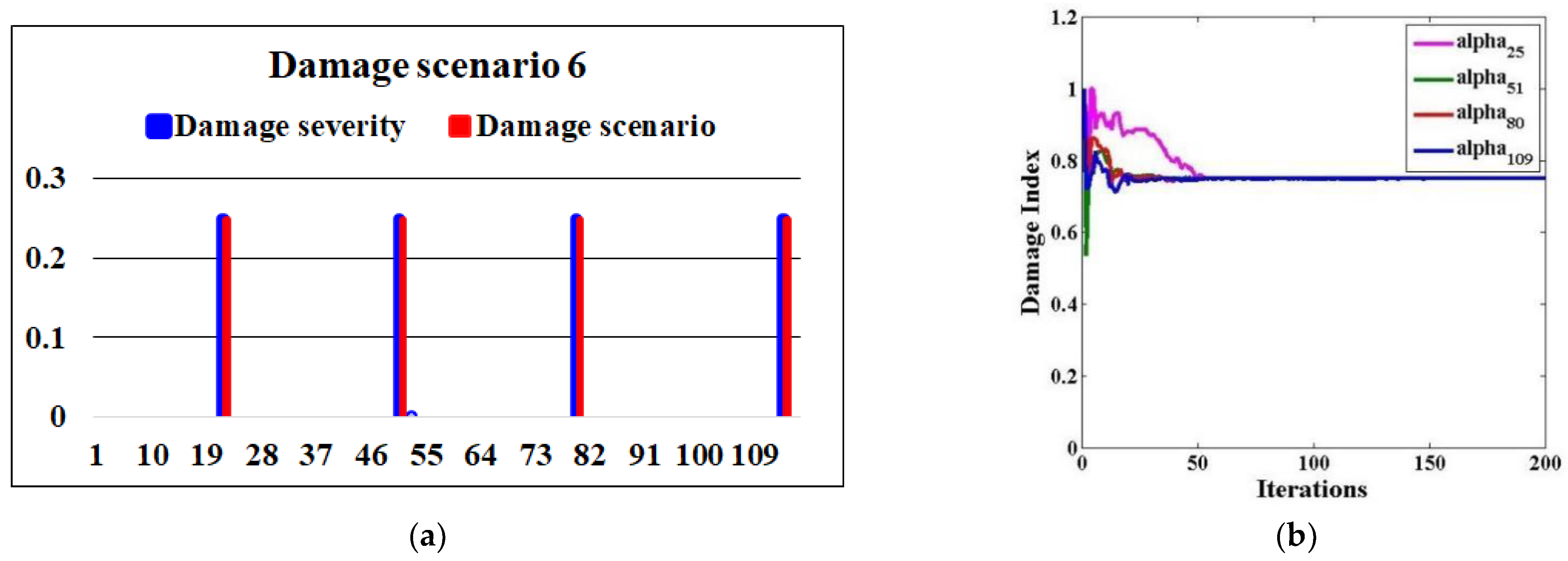
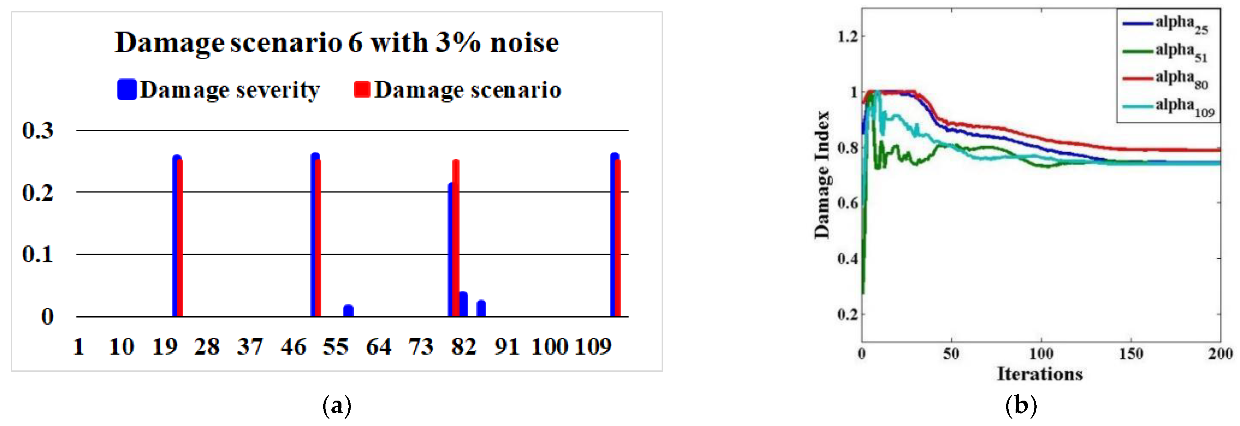
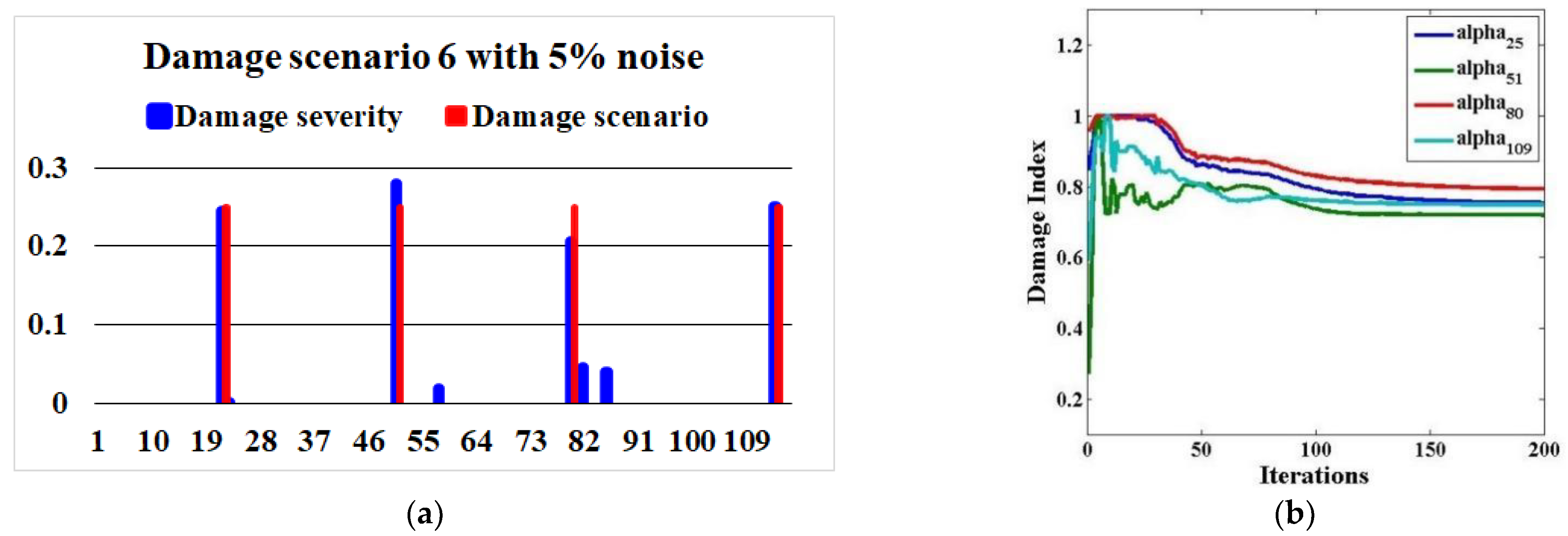
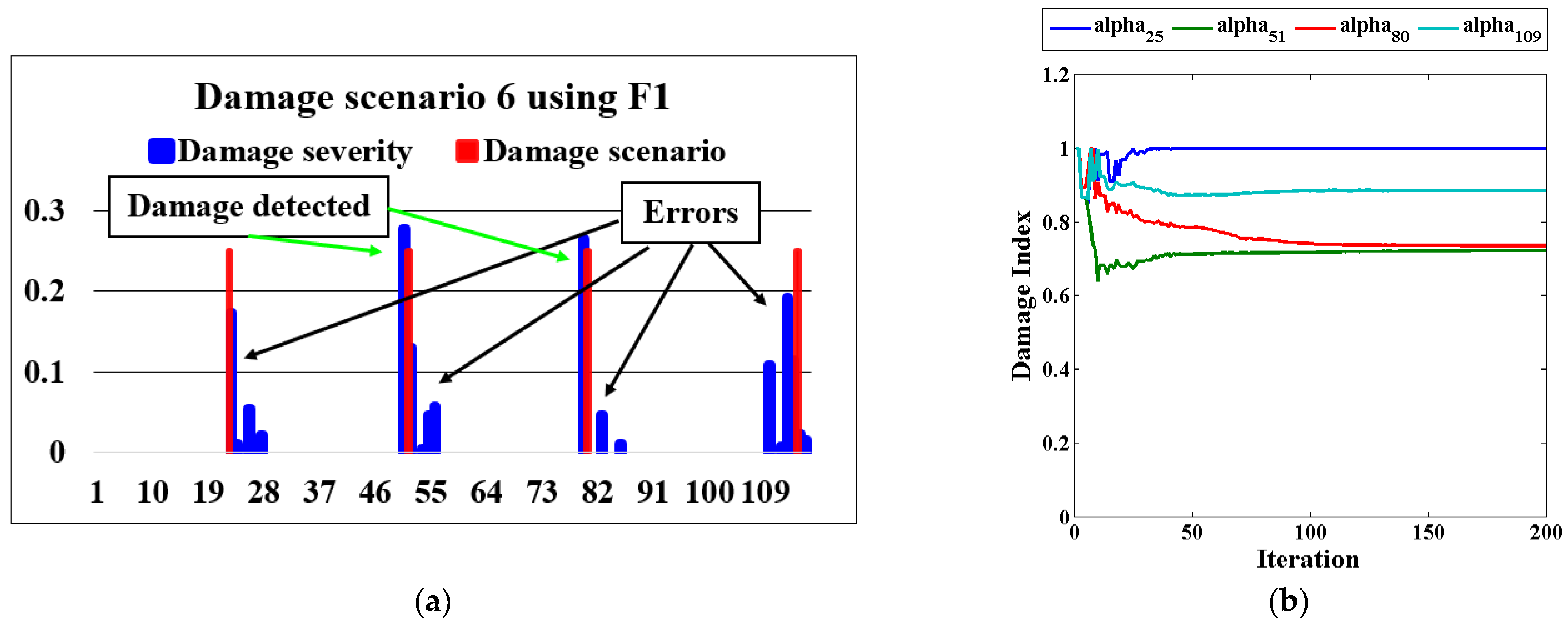
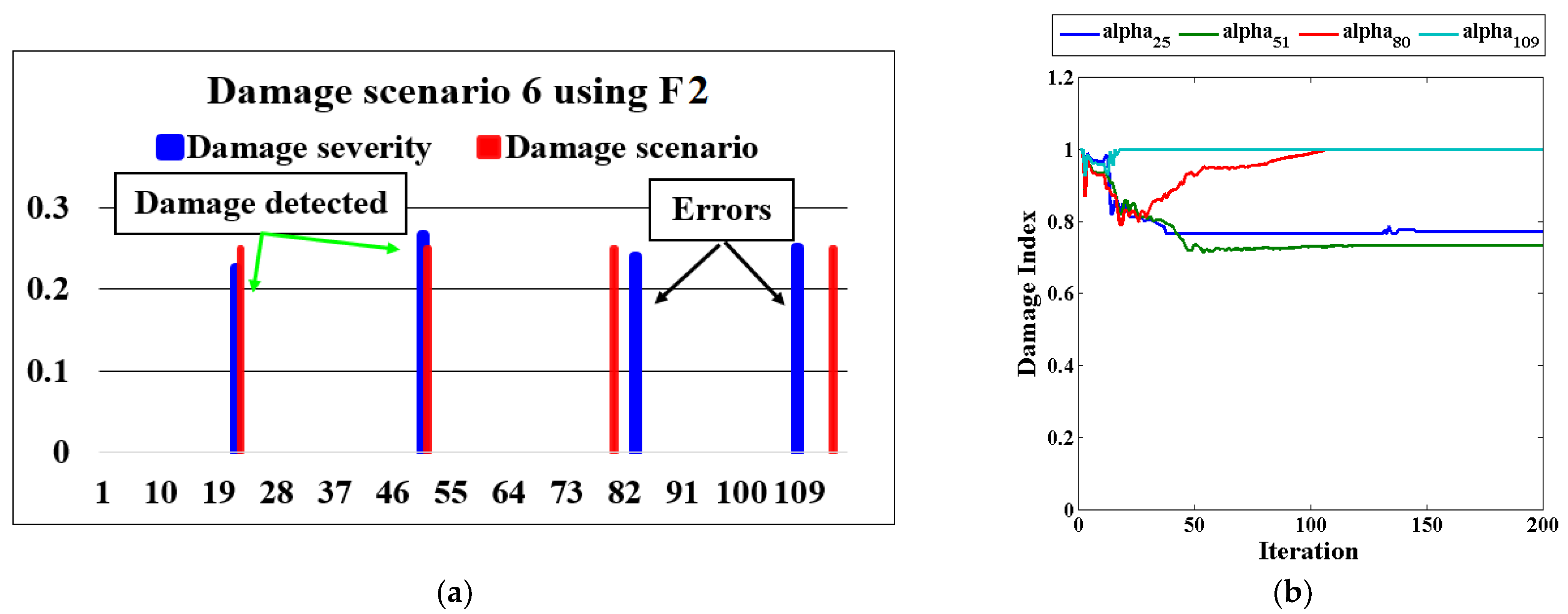
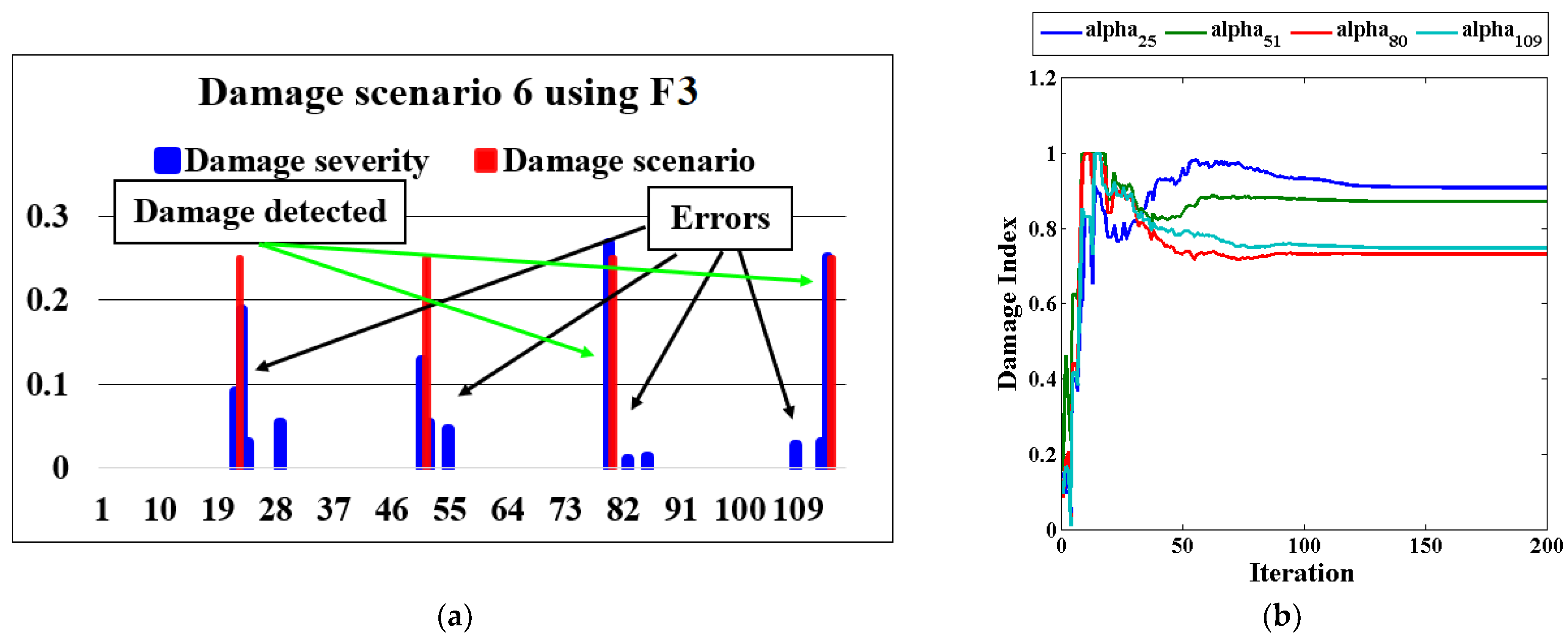
| Scenario 6 | Brace elements 22, 51, 80, and 109 | 25% |
| Damage Scenario | Algorithm | Mean | Standard Deviation | Min | Max | Wilcoxon Sign Rank (p-Value) |
|---|---|---|---|---|---|---|
| Scenario 1 | UPSO | 5.7 × 10⁻⁴ | 5.7 × 10⁻⁴ | 6.5 × 10⁻⁶ | 1.2 × 10⁻³ | 3.9 × 10⁻³ |
| GBO | 6.3 × 10⁻³ | 2.3 × 10⁻⁴ | 6.1 × 10⁻³ | 6.5 × 10⁻³ | 9.0 × 10⁻³ | |
| OL-UPSGBO | 1.1 × 10⁻⁶ | 2.2 × 10⁻⁶ | 6.2 × 10⁻⁷ | 6.5 × 10⁻⁶ | ||
| Scenario 2 | UPSO | 1.3 × 10⁻² | 1.4 × 10⁻⁵ | 1.3 × 10⁻² | 1.3 × 10⁻² | 9.0 × 10⁻³ |
| GBO | 1.6 × 10⁻² | 4.8 × 10⁻³ | 1.1 × 10⁻² | 2.1 × 10⁻² | 9.0 × 10⁻³ | |
| OL-UPSGBO | 9.3 × 10⁻⁸ | 1.1 × 10⁻⁷ | 4.9 × 10⁻⁷ | 2.8 × 10⁻⁷ | ||
| Scenario 3 | UPSO | 5.3 × 10⁻³ | 1.1 × 10⁻⁴ | 5.2 × 10⁻³ | 5.4 × 10⁻³ | 9.0 × 10⁻³ |
| GBO | 6.8 × 10⁻² | 5.4 × 10⁻⁴ | 6.8 × 10⁻² | 6.9 × 10⁻² | 3.9 × 10⁻³ | |
| OL-UPSGBO | 5.5 × 10⁻⁷ | 8.2 × 10⁻⁷ | 3.2 × 10⁻⁸ | 2.0 × 10⁻⁶ | ||
| Scenario 4 | UPSO | 1.3 × 10⁻² | 3.0 × 10⁻⁵ | 1.3 × 10⁻² | 1.3 × 10⁻² | 3.9 × 10⁻³ |
| GBO | 5.3 × 10⁻² | 1.7 × 10⁻² | 4.1 × 10⁻² | 7.6 × 10⁻² | 3.9 × 10⁻³ | |
| OL-UPSGBO | 3.9 × 10⁻⁶ | 4.6 × 10⁻⁶ | 8.8 × 10⁻⁸ | 1.2 × 10⁻⁵ | ||
| Scenario 5 | UPSO | 3.5 × 10⁻² | 3.7 × 10⁻⁴ | 3.5 × 10⁻² | 3.5 × 10⁻² | 3.9 × 10⁻³ |
| GBO | 2.8 × 10⁻² | 1.9 × 10⁻³ | 2.7 × 10⁻² | 3.3 × 10⁻² | 9.1 × 10⁻³ | |
| OL-UPSGBO | 2.2 × 10⁻⁵ | 3.1 × 10⁻⁶ | 1.9 × 10⁻⁵ | 2.6 × 10⁻⁵ | ||
| Scenario 6 | UPSO | 1.3 × 10⁻² | 1.9 × 10⁻⁵ | 1.3 × 10⁻² | 1.3 × 10⁻² | 3.9 × 10⁻³ |
| GBO | 2.3 × 10⁻² | 7.3 × 10⁻⁴ | 2.3 × 10⁻² | 2.4 × 10⁻² | 3.9 × 10⁻³ | |
| OL-UPSGBO | 1.6 × 10⁻⁶ | 1.9 × 10⁻⁶ | 1.9 × 10⁻⁸ | 5.2 × 10⁻⁶ | ||
| Scenario 6 (3% noise) | UPSO | 1.3 × 10⁻² | 2.5 × 10⁻⁵ | 1.3 × 10⁻² | 1.3 × 10⁻² | 3.9 × 10⁻³ |
| GBO | 2.5 × 10⁻² | 1.1 × 10⁻⁵ | 2.5 × 10⁻² | 2.5 × 10⁻² | 3.9 × 10⁻³ | |
| OL-UPSGBO | 4.0 × 10⁻⁴ | 7.5 × 10⁻⁷ | 4.0 × 10⁻⁴ | 4.0 × 10⁻⁴ | ||
| Scenario 6 (5% noise) | UPSO | 1.3 × 10⁻² | 2.7 × 10⁻⁵ | 1.3 × 10⁻² | 1.3 × 10⁻² | 3.9 × 10⁻³ |
| GBO | 2.5 × 10⁻² | 5.3 × 10⁻⁴ | 2.5 × 10² | 2.6 × 10⁻⁴ | 3.9 × 10⁻³ | |
| OL-UPSGBO | 5.8 × 10⁻⁴ | 4.0 × 10⁻⁶ | 5.8 × 10⁻⁴ | 5.9 × 10⁻⁴ |
Publisher’s Note: MDPI stays neutral with regard to jurisdictional claims in published maps and institutional affiliations. |
© 2022 by the authors. Licensee MDPI, Basel, Switzerland. This article is an open access article distributed under the terms and conditions of the Creative Commons Attribution (CC BY) license (https://creativecommons.org/licenses/by/4.0/).
Share and Cite
Alkayem, N.F.; Shen, L.; Al-hababi, T.; Qian, X.; Cao, M. Inverse Analysis of Structural Damage Based on the Modal Kinetic and Strain Energies with the Novel Oppositional Unified Particle Swarm Gradient-Based Optimizer. Appl. Sci. 2022, 12, 11689. https://doi.org/10.3390/app122211689
Alkayem NF, Shen L, Al-hababi T, Qian X, Cao M. Inverse Analysis of Structural Damage Based on the Modal Kinetic and Strain Energies with the Novel Oppositional Unified Particle Swarm Gradient-Based Optimizer. Applied Sciences. 2022; 12(22):11689. https://doi.org/10.3390/app122211689
Chicago/Turabian StyleAlkayem, Nizar Faisal, Lei Shen, Tareq Al-hababi, Xiangdong Qian, and Maosen Cao. 2022. "Inverse Analysis of Structural Damage Based on the Modal Kinetic and Strain Energies with the Novel Oppositional Unified Particle Swarm Gradient-Based Optimizer" Applied Sciences 12, no. 22: 11689. https://doi.org/10.3390/app122211689