An Interface-Corrected Diffuse Interface Model for Incompressible Multiphase Flows with Large Density Ratios

Abstract

An interface-corrected diffuse interface method is presented in this work for the simulation of incompressible multiphase flows with large density ratios. In this method, an interface correction term together with a mass correction term is introduced into the diffuse-interface Cahn–Hilliard model to maintain both mass conservation and interface shapes between binary fluids simultaneously. The interface correction term is obtained by connecting the signed distance functions in the Hamilton–Jacobian equation with the order parameter of the Cahn–Hilliard model. In addition, an improved multiphase lattice Boltzmann flux solver is introduced, in which the fluxes are obtained by considering the contributions of the particle distribution functions before and after the streaming process through a local switch function. The proposed method is validated by simulating multiphase flows, such as the Laplace law, the evolution of a square bubble, the merging of two bubbles, Rayleigh–Taylor instability, and a droplet impacting on a film with a density ratio of 1000. Numerical results show that the presented method can not only reduce the interface diffusion but also has good control over the interface thickness and mass conservation. The improved numerical method has great potential for use in practical applications involving multiphase flows.

1. Introduction

As an important class of flow problems involving two or more fluids, multiphase flows exist widely in nature, as well as in industrial applications, such as droplets hitting a fluid or solid surface, bubble deformation in liquids, and gas-liquid flows in pipes in oil exploitation. In order to simulate multiphase flows, many methods, including the volume of fluid (VOF) method [1,2], the level set method [3,4], the front tracking method [5,6,7], and the diffuse interface (DI) method [8,9], have been proposed. The VOF method is able to capture the phase interface accurately [1,2]. The level set method applies a signed distance function to indicate different phases [3,4]. The front tracking method has the advantage of accurately capturing phase interfaces with small or moderate changes in a very simple way [6,7]. However, maintaining mass conservation is still challenging in multiphase flow simulations. DI methods have been widely applied in recent years due to their firm theoretical basis in the phase field method and advantages in dealing with the complicated evolution of the interface among different fluids, and they have been successfully applied to the Rayleigh–Taylor instability in binary fluids [10], bubbles rising or merging in liquids [11], droplet deformation on impact [12], and so on. Like other numerical methods, the DI methods have two important aspects for simulating multiphase flows: the solution of the flow field and the tracking of the fluid interfaces.

For the solution of the flow field, current methods are usually classified into two types; i.e., the continuum method and the mesoscopic method, based on the gas kinetic theory. The continuum method is carried out by solving the Navier–Stokes (N–S) equations with the finite difference method, finite volume method, and/or finite element method. The continuum methods include those initially developed by Gurtin et al. [13] and Boyer [14]. Different from the continuum method, the mesoscopic kinetic method, which is also called the lattice Boltzmann method (LBM), is realized by solving the lattice Boltzmann equations. The LBM originated from lattice gas automata [15], and now it has developed into a very useful approach to solve complex multiphase flow problems. The LBM also has the advantage of being able to compute multiphase flow with complicated geometric shapes. Many LB models [16,17,18] have been proposed, such as the color model [19]; the interparticle-potential model [20]; the thermodynamically consistent model [21]; the double-distribution-function model (DDF), which includes pressure and density [22]; the projection-like pseudo-potential model [23]; the stable-discretization DDF model [24]; the three-distribution-function model, which includes phase, velocity, and temperature [25]; and the improved single-relaxation-time model [26].

Recently, multiphase lattice Boltzmann flux solvers (MLBFSs) [10,27,28,29] have also been developed and applied to many complex multiphase flow problems, such as the adaptive mesh refinement multiphase lattice Boltzmann flux solver (AMR-MLBFS) developed by Yuan et al. [27] and the improved multiphase lattice Boltzmann flux solver (IMLBFS) developed by Yang et al. [28]. In the MLBFS, the flow properties are directly updated at each cell center and the fluxes are calculated locally at cell surfaces through local reconstruction of lattice Boltzmann solutions. The fluxes are obtained through the operations of equilibrium and non-equilibrium particle distribution functions conforming to the lattice Boltzmann equations. This means that the particle distribution functions are obtained after the streaming and collision process and numerical diffusion can be brought into the MLBFS in the process of flux computation. However, numerical diffusion is not enough, and this affects the computation of the MLBFS, resulting in a larger value for the characteristic velocity for simulating multiphase flows at large density ratios. The efficiency of the computation is thus limited. In order to address this disadvantage, a new flux reconstruction scheme is proposed in this work using particle distribution functions both before and after the collision. A local switch function related to the order parameter is also applied to adjust these particle distribution functions obtained before and after the collision. With this switch function, numerical diffusion can be controlled and the fluxes can be evaluated according to the characteristics of the local multiphase flows.

Besides the flow field, fluid interfaces are solved with the DI method, which also needs improvement. In general, the mass conservation in the DI method cannot be exactly guaranteed, and much effort has been invested in solving this problem. Van der Sman et al. [30] found that a droplet in the shear flow would shrink gradually. Zheng et al. [31] analyzed a two-phase model and found that the static bubble or droplet showed some spontaneous shrinkage phenomena and could even disappear eventually. Some researchers [32,33] opted for an improved mesh to overcome the issue. Ding et al. [33] adopted a dual-resolution Cartesian grid to simulate multiphase problems, solving the flow field on a lower resolution grid while solving the phase field on a higher resolution grid. However, choosing the high-resolution grid often increases the computation cost, and the mass non-conservation issue still exists. Researchers have proposed improved models and methods [34,35,36]. Chao et al. [34] proposed a method with the mass correction procedure based on the He–Chen–Zhang lattice Boltzmann equation. Wang et al. [35] solved the mass conservation issue by introducing the mass-conserved term into the Cahn–Hilliard (C–H) equation and, on this basis, Yang et al. [36] proposed a mass-conserved fractional step axisymmetric lattice Boltzmann flux solver. However, capturing interface inaccuracy in some local places has not been fully resolved yet. Specifically, the thickness of the fluid interface cannot be maintained due to convection and diffusion, so the calculation of surface tension force is not accurate and numerical stability is also affected. In order to overcome this, many methods [37,38,39] have been proposed. Li et al. [37] proposed an improved interfacial profile-corrected C–H model. Zhang et al. [38] proposed a phase-field method that involves correcting the flux. Soligo et al. [39] proposed two improved phase-field method formulations based on the profile-corrected and flux-corrected guidelines. Wang et al. [40] combined the level set method with the DI method by introducing re-initialization to reconstruct the phase interface. Zhang et al. [41] proposed an interface-compressed method applying the gradient of the normal velocity of the local interface. Currently, methods for improving the interfacial condition are still being developed.

In this study, we aimed to develop an interface-corrected DI method with an improved MLBFS for simulating incompressible multiphase flows with large density ratios. Two important improvements were made: one for the DI, allowing it to maintain the equilibrium shape and the thickness of the fluid interface; and the other for the MLBFS, allowing it to evaluate the fluxes according to the characteristics of the local multiphase flows. To enforce the shape and thickness of the fluid interface during the dynamic evolution of the flow field, an interface correction term is introduced into the DI model by applying the Hamilton–Jacobi equation. This term only takes into account effects around the fluid interfaces between different phases. The fluxes are reconstructed by applying the particle distribution functions both before and after collisions. A local switch function is also introduced to automatically adjust the contributions of these distribution functions to the fluxes. Moreover, a mass correction term is also introduced into the DI model. The proposed method was validated by simulating several multiphase flow benchmarks, inducing the Laplace law, the evolution of the square bubble, the merging of two bubbles, the Rayleigh–Taylor instability, and a droplet splashing on a thin film with a density ratio of 1000. In Section 2, the methodology for the solutions for both the phase field and the flow field is presented. In Section 3, the numerical results are presented to validate the proposed method, along with a discussion. In Section 4, the conclusions of the present work are drawn.

2. Methodology

2.1. Improved Mass-Conserved and Interface-Corrected DI Method

2.1.1. Original Cahn–Hilliard Model

In the original DI method, the Cahn–Hilliard model is often adopted to trace the interfaces in the calculation. The governing equation of the original model can be written as:

$$\frac{\partial C}{\partial t}+\nabla \cdot \left(\mathit{u}C\right)=\mathrm{\Gamma }{\nabla }^2{\mu }_C,$$

(1)

where $C$ is the volume fraction of heavier fluids for two-phase flows in the range of [0, 1], which is also named as the order parameter; $t$ is time; $\mathit{u}$ is the velocity of the fluid; $\mathrm{\Gamma }$ is the mobility; and ${\mu }_C$ is the chemical potential obtained from the free energy in the interfaces, and it can be written as:

$${\mu }_C=2\beta C\left(C-1\right)\left(2C-1\right)-\kappa {\nabla }^{2}C,$$

(2)

Here, the constants $\beta$ and $\kappa$ are obtained from the surface tension coefficient $\sigma$, as well as the interface thickness parameter $\xi$:

$$\kappa =\frac{3}{2}\sigma \xi ;\hspace{1em}\beta =\frac{12\sigma }{\xi },$$

(3)

Based on the order parameter $C$, the local density $\rho$ of the fluid can be obtained from a linear combination of the heavier and lighter fluids (${\rho }_H$ and ${\rho }_L$):

$$\rho ={\rho }_L+C\mathrm{\Delta }\rho ;\hspace{1em}\mathrm{\Delta }\rho ={\rho }_H-{\rho }_L,$$

(4)

Many numerical methods [10,32] have been developed to discretize the Cahn–Hilliard Equation (Equation (1)) for tracking fluid interfaces. However, numerical and/or modeling errors, such as diffusion and dissipation, flatten or compress the fluid interfaces such that unphysical results can be obtained during numerical simulations. In the present study, inspired by the Hamilton–Jacobian equation used in the level set method, a new correction term is introduced into the original Cahn–Hilliard model to maintain the shape of the fluid interface. In addition, to guarantee mass conservation, a mass correction term, introduced previously by Wang et al. [35], is also applied.

2.1.2. Improved Cahn–Hilliard Model with Mass Conservation and Interface Correction

This section presents a development of the improved Cahn–Hilliard model to effectively capture the phase interface. In order to maintain the equilibrium shape, as well as the thickness of the fluid interface, and guarantee mass conservation, an interface correction term $q_1$ and a mass conservation term $q_2$ are adopted in the C–H model. The modified C–H model with mass conservation and interface correction can be written as:

$$\frac{\partial C}{\partial t}+\nabla \cdot (\mathit{u}C)=\mathrm{\Gamma }{\nabla }^2{\mu }_C-q_1+q_2,$$

(5)

where $q_1$ is introduced to maintain the shape of the phase interface and $q_2$ is used to guarantee mass conservation. The interfacial shape can be obtained analytically in the one-dimensional case by using the free energy density model for immiscible two-phase flows:

$$C\left(d\right)=\frac{1}{2}\left[1+\tanh \left(\frac{2d}{\xi }\right)\right],$$

(6)

where $d$ is the signed distance along the gradient of $C$. It ought to be noticed that the surface tension force is obtained by assuming that the interface shape follows Equation (6) during the evolution of the fluid interfaces. This means that, when the shape of the interface is different from that described by Equation (6), the surface tension cannot be obtained accurately. However, the DI model is not able to guarantee the local shape of the interface in unsteady flow simulations, especially if the density ratio of fluids is huge and the convective effect is strong. It should be noted that the level set approach can quite easily maintain the interfacial shape, since the signed distance function $d$ is obtained accurately by applying the Hamilton–Jacobian equation, which can be written as:

$$\frac{\partial d}{\partial \tau }+S\left(d\right)\left(\left|\nabla d\right|-1\right)=0,$$

(7)

$$S\left(d\right)=\frac{d}{\sqrt{{\left(d\right)}^2+{\left(\left|\nabla d\right|\epsilon \right)}^2}},$$

(8)

where $\tau$ is the pseudo time, $S\left(d\right)$ is a smoothed signed function, and $\epsilon$ is equal to the mesh size $\mathrm{\Delta }x$ in this paper.

Inspired by the level set approach, where the Hamilton–Jacobian equation is applied to accurately calculate the signed distance equation, the interface correction term $q_1$ is introduced into the Cahn–Hilliard model, which can be written as:

$$q_1=kS\left(d\right)\left(\left|\nabla d\right|-1\right),$$

(9)

Here, $k$ is a constant connected with the mesh size $\mathrm{\Delta }x$ and the characteristic length $L$. It ought to be noticed that $q_1$ only works in the interfacial layer, while it is zero elsewhere. To get the expression of the source term $q_1$ explicitly in terms of the order parameter, the signed distance function $d$ can be expressed by using the order parameter with the aid of Equation (6):

$$d=\frac{\xi }{2}{\tanh }^{-1}\left[2\left(C-0.5\right)\right],$$

(10)

Equation (10) implies that the signed $d=0$ and the interface of the order parameter $C=0.5$ both represent the phase interface. In our research, in order to avoid a numerical error, the interface correction term $q_1$ is applied in the zone of $0.01\le C\le 0.99$. Substituting Equation (10) into Equation (9) gives the final expression of the source term $q_1$.

$$q_1=\left\{\begin{array}{cc}\frac{k\ln \left(\frac{C}{1-C}\right)}{\sqrt{{\left(\ln \left(\frac{C}{1-C}\right)\right)}^2+{\left(\left|\frac{1}{C-C^2}\right|\left|\nabla C\right|\epsilon \right)}^2}}\left(\left|\frac{\xi }{4C-4C^2}\right|\left|\nabla C\right|-1\right),\hfill & \hspace{1em}\mathrm{if}(0.01\le C\le 0.99)\hfill \\ \hspace{1em}\hspace{1em}0,\hfill & \mathrm{elsewhere}\hfill \end{array}\right.$$

(11)

In addition to the interface shape correction term $q_1$, the mass conservation term $q_2$ is obtained by assuming that this term exists averagely in the interfacial layer. It can thus be obtained by integrating Equation (5) in the zone ${\mathrm{\Omega }}_L$ filled with lighter fluid. The derived equation can be written as:

$${\displaystyle \underset{{\mathrm{\Omega }}_L}{\mathrm{\int }}\frac{\partial C}{\partial t}}dV+{\displaystyle \underset{S}{\mathrm{\int }}\left(\mathit{u}C\right)\cdot } d\mathit{S}={\displaystyle \underset{{\mathrm{\Omega }}_L}{\mathrm{\int }}\mathrm{\Gamma }}{\nabla }^2{\mu }_{C}dV-{\displaystyle \underset{{\mathrm{\Omega }}_L}{\mathrm{\int }}{q}_1}dV+{\displaystyle \underset{{\mathrm{\Omega }}_L}{\mathrm{\int }}{q}_2}dV,$$

(12)

Here, $S$ represents the border of the zone ${\mathrm{\Omega }}_L$. The term ${\displaystyle \underset{S}{\mathrm{\int }}\left(\mathit{u}C\right)\cdot }d\mathit{S}$ ought to be zero due to conservation of mass; i.e., there is no mass transfer across the interface:

$${\displaystyle \underset{S}{\mathrm{\int }}\left(\mathit{u}C\right)\cdot } d\mathit{S}=0,$$

(13)

Furthermore, by using Equation (4), the following relationship can be found:

$${\displaystyle \underset{{\mathrm{\Omega }}_L}{\mathrm{\int }}\frac{\partial C}{\partial t}}dV=\frac{1}{\mathrm{\Delta }\rho }\cdot \frac{\partial }{\partial t}{\displaystyle \underset{{\mathrm{\Omega }}_L}{\mathrm{\int }}\rho dV}=\frac{1}{\mathrm{\Delta }\rho }\cdot \frac{\partial M_L}{\partial t},$$

(14)

where $M_L$ is the mass of the lighter fluid.

It ought to be noticed that the mass correction term $q_2$ is only applied in the interface layer. By using Equations (12)–(14), the term $q_2$ can be written as:

$$q_2=\left\{\begin{array}{cc}\frac{1}{\mathrm{\Delta }V}\left(\frac{1}{\mathrm{\Delta }\rho }\frac{\partial M_L}{\partial t}-{\displaystyle \underset{{\mathrm{\Omega }}_L}{\mathrm{\int }}\mathrm{\Gamma }{\nabla }^2{\mu }_{C}dV+{\displaystyle \underset{{\mathrm{\Omega }}_L}{\mathrm{\int }}{q}_{1}dV}}\right),\hfill & 0<C<1\hfill \\ \hspace{1em}\hspace{1em}0,\hfill & \mathrm{elsewhere}\hfill \end{array}\right.,$$

(15)

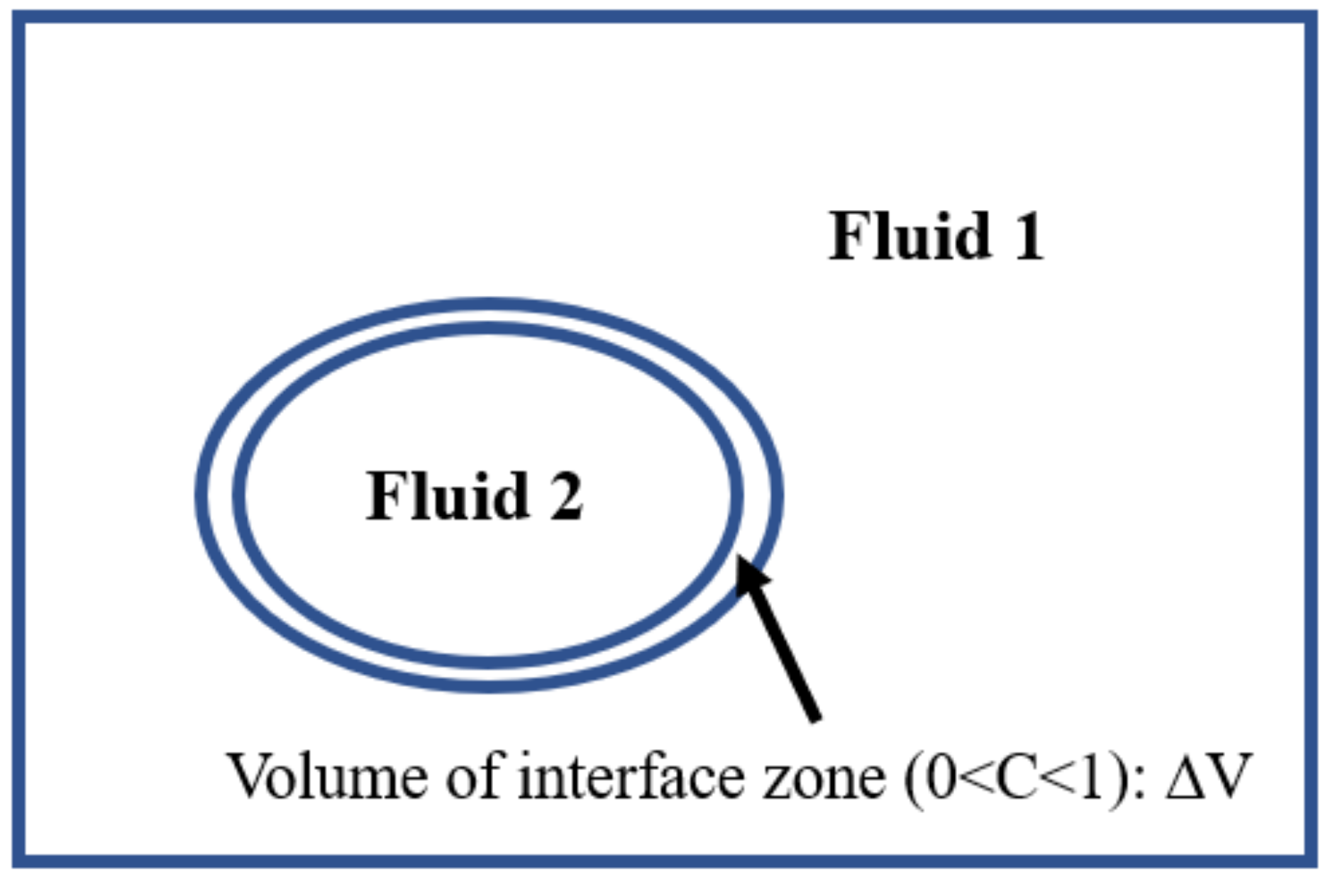
where $\mathrm{\Delta }V$ is the volume of the interfacial zone, as shown in Figure 1. It should be noted that the term $\mathrm{\Gamma }{\nabla }^2{\mu }_C=0$ is applied in areas away from the interface layer. In the present study, the source term $q_2$ only works to reduce the errors of analyzing the interface layer if $0.001\le C\le 0.999$, and it is finally written as:

$$q_2=\left\{\begin{array}{cc}\frac{1}{\mathrm{\Delta }V}\cdot \left(\frac{\mathrm{\Delta }M}{\mathrm{\Delta }\rho \cdot \mathrm{\Delta }t}-{\displaystyle \sum _{{\mathrm{\Omega }}_L}\mathrm{\Gamma }{\nabla }^2{\mu }_C\cdot dV+{\displaystyle \sum _{{\mathrm{\Omega }}_L}{q}_1}}\cdot dV\right),\hfill & \mathrm{if}(0.001\le C\le 0.999)\hfill \\ \hspace{1em}\hspace{1em}0,\hfill & \mathrm{elsewhere}\hfill \end{array}\right.$$

(16)

where $\mathrm{\Delta }M=M^n-M^0$, $\mathrm{\Delta }t$ is the time step during the calculation, $M^0$ is the total mass of the lighter fluid for two-phase flows at $t=t_0$, and $M^n$ is the total mass of the lighter fluid at $t=t_n$.

$$M^n={\displaystyle \underset{C\le 0.5}{\mathrm{\int }}\rho dV={\rho }_L}{V}_L^n,$$

(17)

So far, a modified Cahn–Hilliard model with mass conservation and interface correction has been constructed. In this paper, we use the second-order central difference scheme to discretize the term $\mathrm{\Gamma }{\nabla }^2{\mu }_C$, and the second-order Lax–Wendroff scheme to discretize the term $\nabla \cdot (\mathit{u}C)$.

2.2. Governing Equations for the Flow Field and the Improved MLBFS

2.2.1. Governing Equations

For effective simulation of incompressible multiphase flows, the governing equations reproduced by the multiphase lattice Boltzmann flux solver [42] can be written as:

$$\frac{\partial \mathit{W}}{\partial t}+\nabla \cdot \mathit{F}=\mathit{S},$$

(18)

where $\mathit{W}={\left(p,\rho u{c}_s^2,\rho v{c}_s^2\right)}^T$; $\rho$ is the fluid density; $c_s$ is the speed of sound given by the lattice velocity model; $u$ and $v$ are, respectively, the fluid velocity components in the $x$ and $y$ directions; $p$ represents the pressure; $\mathit{F}$ represents the flux; and $\mathit{S}$ represents source terms:

$$\mathit{F}={\left({\displaystyle \mathbf{\sum }_{\alpha =0}^N{\mathit{e}}_{\alpha }{f}_{\alpha }^{eq}},{\displaystyle \mathbf{\sum }_{\alpha =0}^N{\mathit{e}}_{\alpha }{\mathit{e}}_{\alpha }{f}_{\alpha }^{\wedge }}\right)}^T,$$

(19)

$$\mathit{S}={\left(-\mathit{u}\cdot \nabla \left(p-\rho c_s^2\right),c_s^2{\mathit{F}}_s\right)}^T,$$

(20)

$$f_{\alpha }^{eq}\left(\mathit{r},t\right)=w_{\alpha }\left[p+\rho c_s^2\left(\frac{{\mathit{e}}_{\alpha }\cdot \mathit{u}}{c_s^2}+\frac{{\left({\mathit{e}}_{\alpha }\cdot \mathit{u}\right)}^2-{\left(c_s\left|\mathit{u}\right|\right)}^2}{2c_s^4}\right)\right],$$

(21)

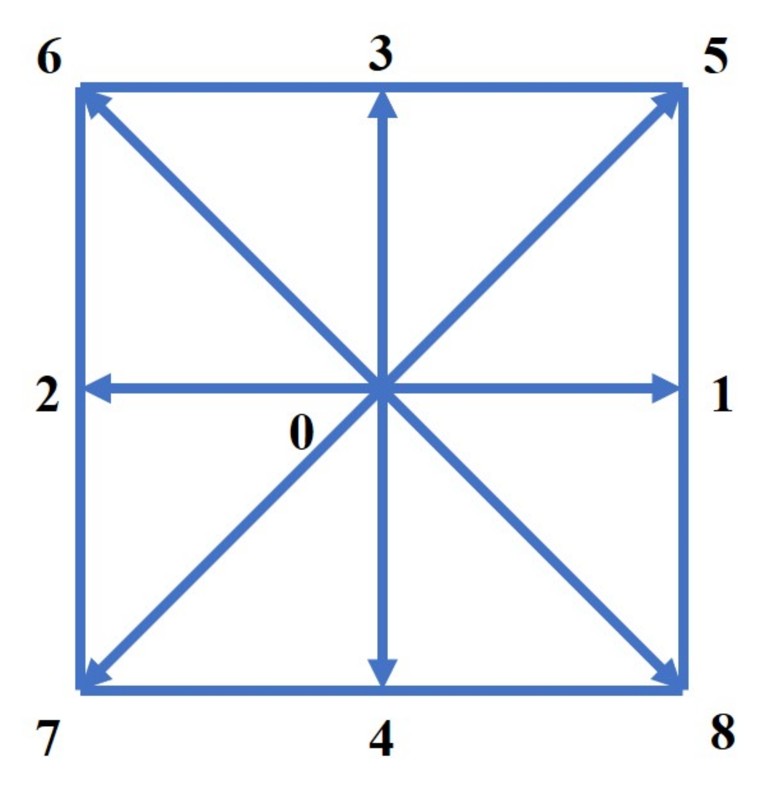
Here, ${\mathit{e}}_{\alpha }$, $N$, $w_{\alpha }$, and $c_s$ are given by the lattice velocity model; ${\mathit{e}}_{\alpha }$ is the particle velocity in the $\alpha$ direction; $N$ is the number of discrete particle velocities; $w_{\alpha }$ are the coefficients; $c_s$ is the speed of sound; $\mathit{r}$ represents a physical location; $f_{\alpha }^{eq}$ is the original equilibrium particle distribution function; $f_{\alpha }^{\wedge }$ is the function of $f_{\alpha }^{eq}$, applied in the flux reconstruction; and ${\mathit{F}}_s$ is the surface tension force. In this article, the lattice velocity model is the D2Q9 model shown in Figure 2: each vector represents the particle velocity in the corresponding direction. The speed of sound $c_s=c/\sqrt{3}$, $c={\delta }_x/{\delta }_t$, ${\delta }_x$ is the lattice spacing, ${\delta }_t$ is the streaming time step, $w_0=4/9$, $w_1=w_2=w_3=w_4=1/9$, and $w_5=w_6=w_7=w_8=1/36$.

The surface tension force ${\mathit{F}}_s$ has many different forms. The potential form from [41] is adopted in the present study, and it is defined as:

$${\mathit{F}}_s={\mu }_C\nabla C,$$

(22)

2.2.2. Finite Volume Discretization

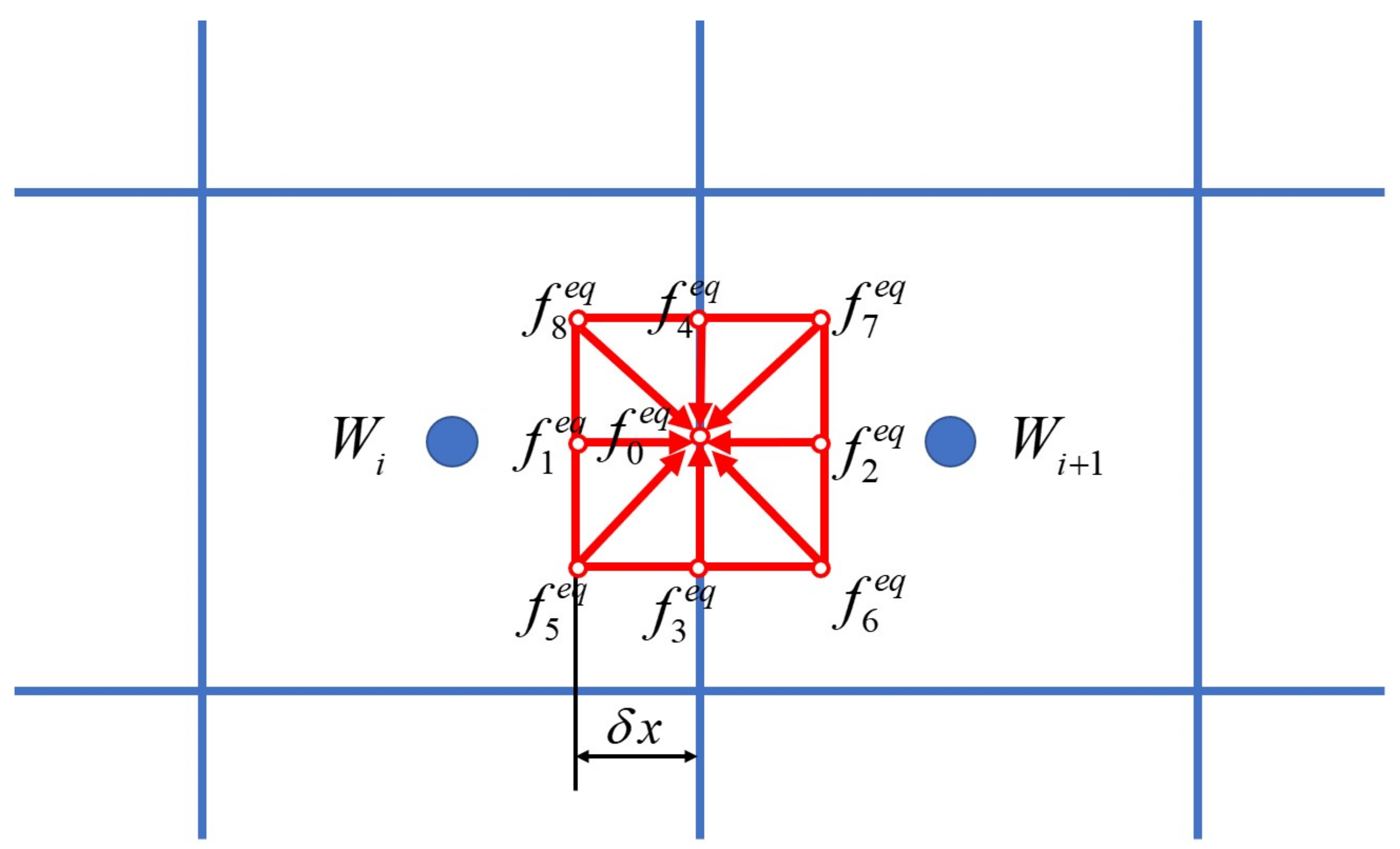
In the study, we adopt the finite volume method to solve Equation (18) and the second-order total variation diminishing (TVD) Runge–Kutta scheme to calculate ($\mathit{W}={\left(p,\rho u{c}_s^2,\rho v{c}_s^2\right)}^T$) at the cell centers. The resulting equations can be written as:

$$\frac{d{\mathit{W}}_i}{dt}=-\frac{1}{{\mathrm{\Omega }}_i}{\displaystyle \mathbf{\sum }_k{\mathit{R}}_k{l}_k}+\mathit{S},$$

(23)

$${\mathit{R}}_k={\left(\mathit{n}\cdot {\displaystyle \mathbf{\sum }{\mathit{e}}_{\alpha }}{f}_{\alpha }^{eq},\mathit{n}\cdot {\displaystyle \mathbf{\sum }{\mathit{e}}_{\alpha }{\mathit{e}}_{\alpha }{f}_{\alpha }^{\wedge }}\right)}^T,$$

(24)

where ${\mathit{W}}_i$ represents the flow variables of the $i$th control volume, ${\mathrm{\Omega }}_i$ is the area of the $i$th control volume, $l_k$ is the length of the $k$th surface of the $i$th control volume, and $\mathit{n}$ is the unit outer normal vector of the $k$th surface. The flux evaluation at a cell interface is shown in Figure 3. In the figure, ${\delta }_x$ is the lattice spacing, $f_{\alpha }^{eq}$ represents the equilibrium particle distribution in different directions, and ${\mathit{W}}_i$, ${\mathit{W}}_{i+1}$ are the flow variables of two adjacent control volumes.

The flux ${\mathit{R}}_k$ at the kth control surface can be finally written as:

$$R_k={\left[\begin{array}{c}{n}_x\left(f_1^{eq}-f_2^{eq}+f_5^{eq}-f_6^{eq}-f_7^{eq}+f_8^{eq}\right)+n_y\left(f_3^{eq}-f_4^{eq}+f_5^{eq}+f_6^{eq}-f_7^{eq}-f_8^{eq}\right)\\ n_x\left(f_1^{^}+f_2^{^}+f_5^{^}+f_6^{^}+f_7^{^}+f_8^{^}\right)+n_y\left(f_5^{^}-f_6^{^}+f_7^{^}-f_8^{^}\right)\\ n_x\left(f_5^{^}-f_6^{^}+f_7^{^}-f_8^{^}\right)+n_y\left(f_3^{^}+f_4^{^}+f_5^{^}+f_6^{^}+f_7^{^}+f_8^{^}\right)\end{array}\right]}_k$$

(25)

where $\mathit{n}=\left(n_x,n_y\right)$ is the unit outward normal vector of the $k$th surface, and $n_x$ and $n_y$ are the $x$ and $y$ components of $\mathit{n}$.

2.2.3. The New Flux Reconstruction Scheme

In previous studies [40,42], the distribution function $f_{\alpha }^{\wedge }$ is approximated by:

$$f_{\alpha }^{\wedge }=f_{\alpha }^{eq}(\mathit{r},t)-\left(\tau -\frac{1}{2}\right)\left[f_{\alpha }^{eq}(\mathit{r},t)-f_{\alpha }^{eq\_m}(\mathit{r}-{\mathit{e}}_{\alpha }{\delta }_t,t-{\delta }_t)\right],$$

(26)

$$f_{\alpha }^{eq}\left(\mathit{r},t\right)=w_{\alpha }\left[p+\rho {\mathrm{\Gamma }}_{\alpha }\right]=w_{\alpha }\left[p+\rho c_s^2\left(\frac{{\mathit{e}}_{\alpha }\cdot \mathit{u}}{c_s^2}+\frac{{\left({\mathit{e}}_{\alpha }\cdot \mathit{u}\right)}^2-{\left(c_s\left|\mathit{u}\right|\right)}^2}{2c_s^4}\right)\right],$$

(27)

$$f_{\alpha }^{eq\_m}(\mathit{r}-{\mathit{e}}_{\alpha }{\delta }_t,t-{\delta }_t)=w_{\alpha }\left[p+\rho (\mathit{r},t-{\delta }_t){\mathrm{\Gamma }}_{\alpha }\right],$$

(28)

It can be seen that $f_{\alpha }^{eq}(\mathit{r},t)$ is the original equilibrium particle distribution function obtained by applying the LBM after the collision, $f_{\alpha }^{eq\_m}$ is the modified equilibrium particle distribution function, $\tau$ is the single relaxation parameter, $\mathit{r}$ is the mid-point of the interface between two adjacent control volumes, and $f_{\alpha }^{eq}(\mathit{r},t)$ is used for calculating the convective fluxes. It may be noted that, due to large density ratios at the phase interface in some multiphase flows and the nonlinearity of the convective terms, numerical instability can occur since not much numerical diffusion is introduced by only considering the distribution function before the collision. Inspired by the previous studies on supersonic compressible flows with shock waves in gas kinetic methods [43,44], the equilibrium particle distribution function before collisions is also applied to calculate the inviscid fluxes:

$$f_{\alpha }^{\wedge }=\left(1-\eta \right)f_{\alpha }^{eq}(\mathit{r},t)+\eta f_{\alpha }^{eq\_m}(\mathit{r}-{\mathit{e}}_{\alpha }{\delta }_t,t-{\delta }_t)-\left(\tau -\frac{1}{2}\right)\left[f_{\alpha }^{eq}(\mathit{r},t)-f_{\alpha }^{eq\_m}(\mathit{r}-{\mathit{e}}_{\alpha }{\delta }_t,t-{\delta }_t)\right]$$

(29)

Here, $\eta =\min (\lambda , 0.025)$, $\lambda =\tanh \left(\left|C_L-C_R\right|/\left(2\left(C_L+C_R+0.2\right)\right)\right)$, $C_L$ is the order parameter of the left control volume for a surface, and $C_R$ is the order parameter of the right control volume. As mentioned earlier, the new scheme includes the particle distribution functions both before and after the collision. A local switch function is also introduced to adjust their contributions in different flow regions. In most of the flow fields without any phase interfaces, the particle distribution after collision contributes more to the inviscid fluxes, as usual, whilst in the interfacial zone, the particle distribution function before collision has a greater effect. Therefore, the numerical diffusion can be controlled and the fluxes can be evaluated according to the characteristics of the local multiphase flows.

2.3. Computational Process

The solution process for the interface-corrected diffuse interface model and the flux solver is shown below:

(1)

Set up the length of ${\delta }_x$ (${\delta }_x={\delta }_t$) at the surfaces of each control volume;

(2)

Based on the flow variables $\rho$, $\mathit{u}$, $p$, and $C$ of each control volume, compute $f_{\alpha }^{eq\_m}(\mathit{r}-{\mathit{e}}_{\alpha }{\delta }_t,t-{\delta }_t)$ applying Equation (28), then acquire $f_{\alpha }^{eq}(\mathit{r},t)$ using Equation (27);

(3)

Compute the fluxes ${\mathit{R}}_k$ at the surfaces using Equation (25) and acquire source terms using Equation (20);

(4)

Compute the interface correction term $q_1$ given by Equation (11) and the mass correction term $q_2$ using Equation (16);

(5)

Discretize Equation (5) by applying the central difference scheme to the diffuse term and the Lax–Wendroff scheme to the convective term;

(6)

Use the second-order TVD Runge–Kutta temporal scheme to solve Equations (5) and (23); in this way, the flow variables of the next time step can be obtained;

(7)

Repeat steps (2–6) until the final results are obtained.

As shown in the above computational sequence, a major improvement was made in this study. For the tracking of the phase interfaces, compared to the original DI model with merely the mass conservation term proposed in [32], the approach proposed in this study has the advantage of maintaining interface shapes. Overall, the proposed approach has good properties for mass conservation and interface correction. It was tested in the next part of the study by simulating several multiphase flow problems.

3. Numerical Results and Discussion

In this part of study, the proposed interface-corrected diffuse interface model together with the improved flow field solver was validated by simulating several multiphase problems, including the Laplace law of a static bubble, the evolution of a square bubble, the process of two bubbles merging under the surface tension force, the Rayleigh–Taylor instability, and the evolution of a droplet splashing on a liquid film. The numerical results obtained with the present method were compared with the reference data and the data obtained with the original method.

3.1. Laplace Law

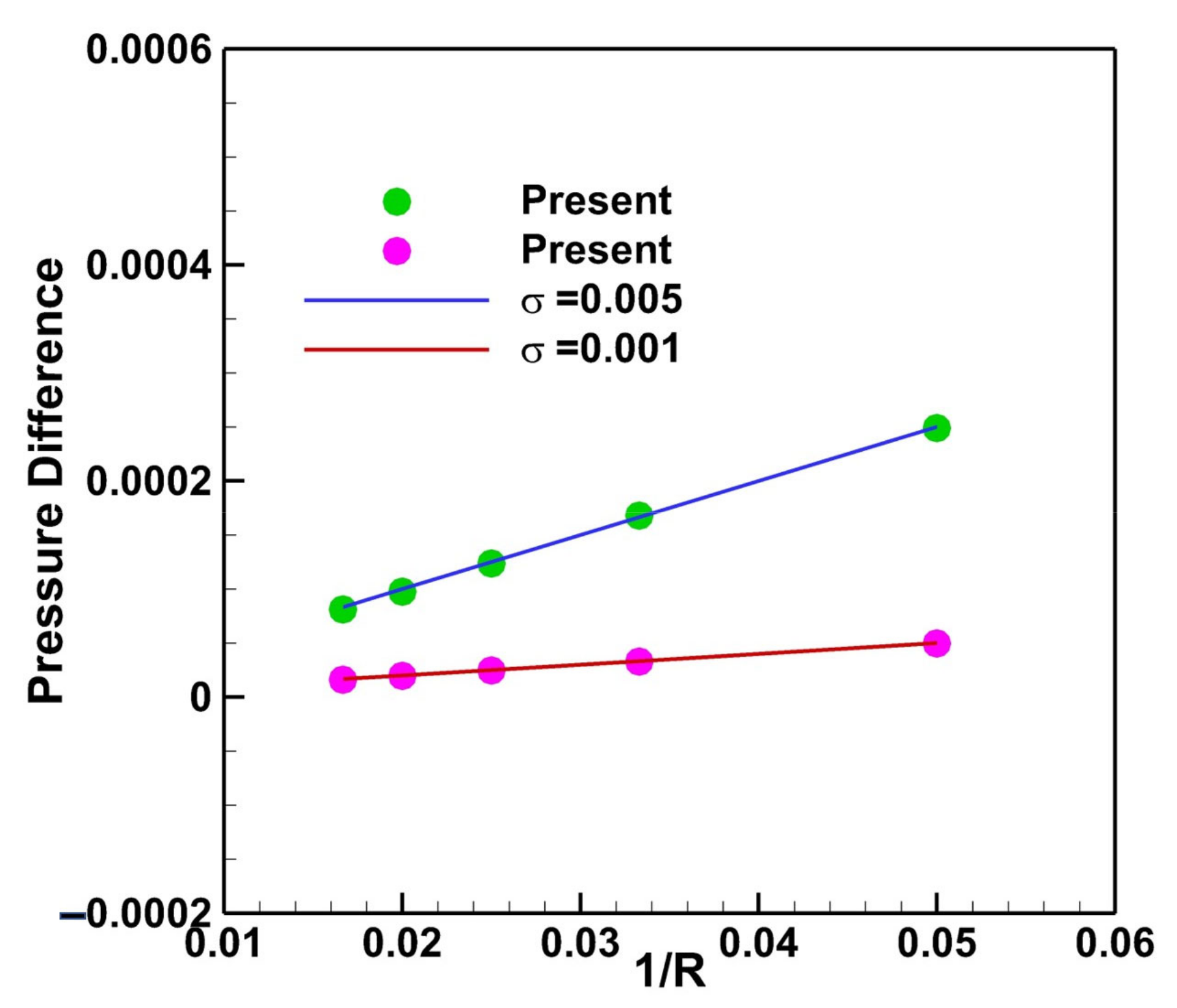
The Laplace law, which considers a light bubble (density ${\rho }_L$) immersed in a heavier fluid (density ${\rho }_H$), was used to test whether the proposed method would have a good influence on mass conservation and interface correction. The law of the pressure and surface tension is written as:

$$p_{in}-p_{out}=\frac{\sigma }{R},$$

(30)

Here, $p_{in}$ is the average pressure inside the bubble, while $p_{out}$ is the average pressure outside, $\sigma$ is the surface tension coefficient, and $R$ is the radius of the bubble. The order parameter $C$ along the normal direction of the phase interface can be obtained with Equation (6).

In this study, the mesh size of $301\times 301$ was adopted for simulation, The natural boundary condition was applied on all walls. The natural boundary condition is that the gradient of all flow variables and the order parameter in the phase field is zero along the outer normal direction of the boundary. In addition, the following parameters were applied in the numerical simulation: ${\rho }_H=10$, ${\rho }_L=1$, and ${\nu }_H={\nu }_L=0.002$, while $R$ was varied from 20 to 60, $\sigma$ was defined as 0.001 and 0.005, and $\xi =3$ for the solutions obtained in Figure 4, Figure 5 and Figure 6. The coefficient $k$ was defined as $k=k_1\mathrm{\Gamma }{\left(\frac{\mathrm{\Delta }x}{L}\right)}^2$ in Equation (11), where $k_1$ was set as $k_1=1$. The characteristic length $L=2R$. For the solution obtained in Figure 7, we set the interface thickness $\xi =3,4,5,6$ in the initial condition to examine the effects of the interface correction terms in the improved C–H equation. It should be noted that Equation (6) was applied to set the order parameter $C\left(d\right)$ in the initial phase field and the theoretical value of the interface thickness of $\xi =3$ was applied to calculate the surface tension.

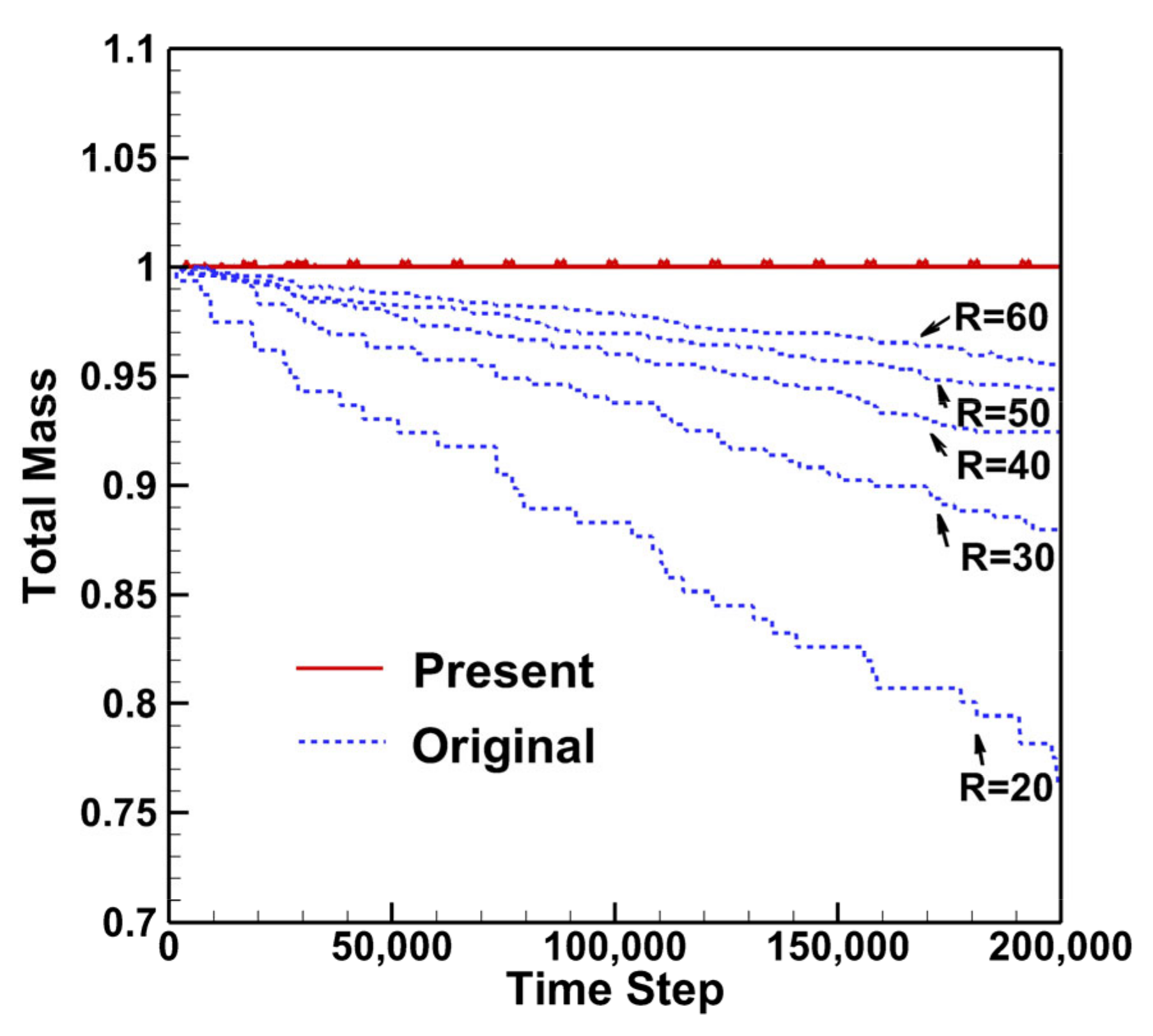
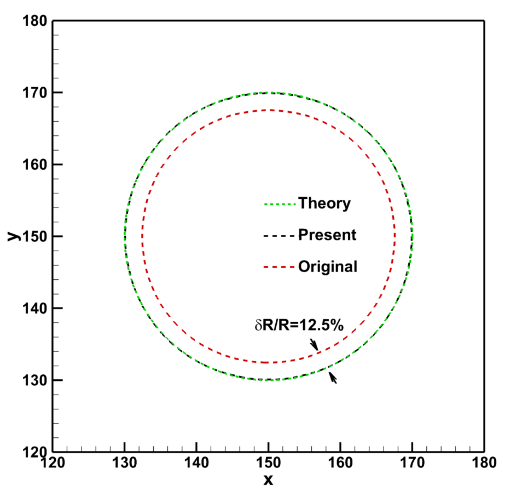
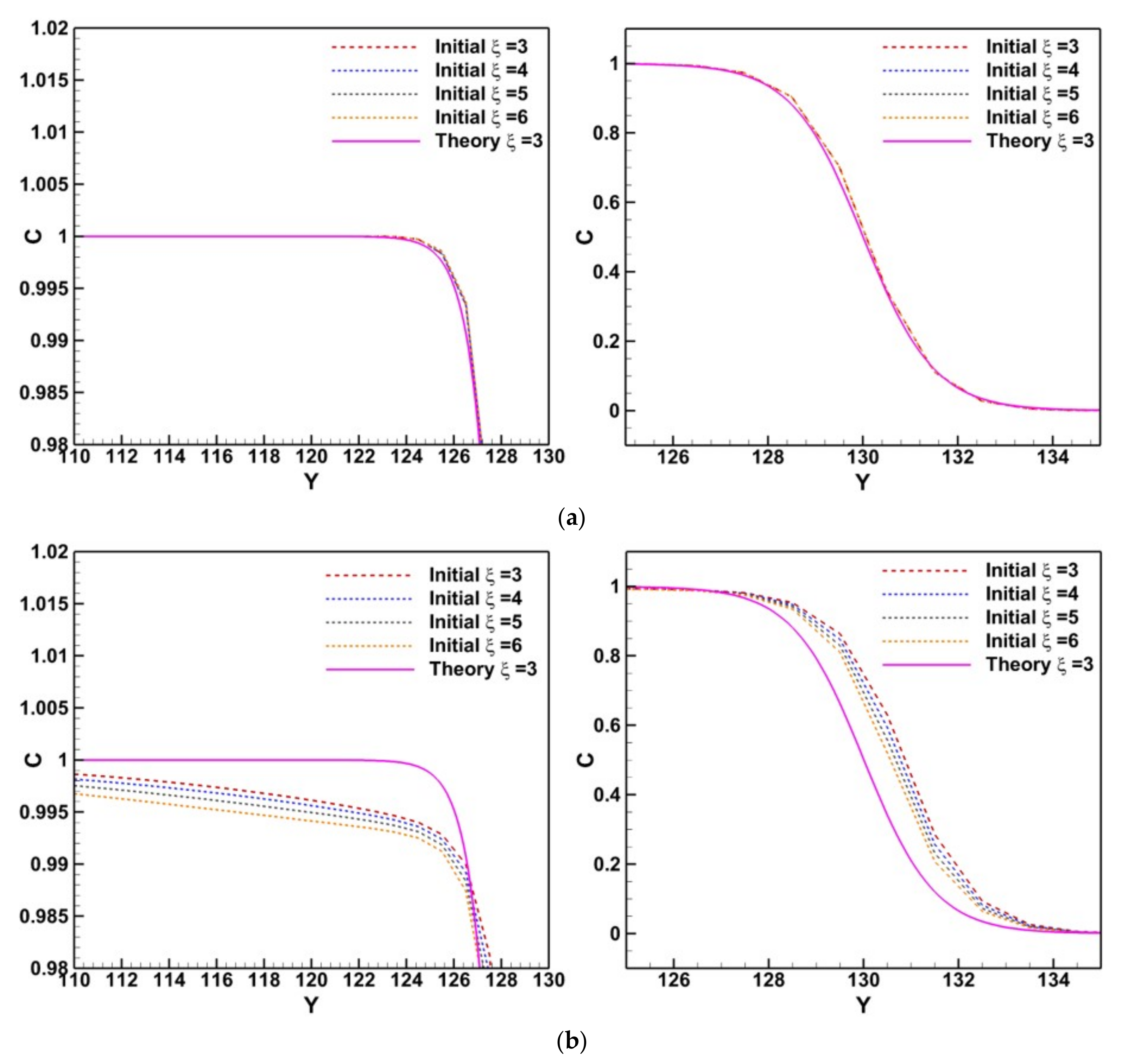
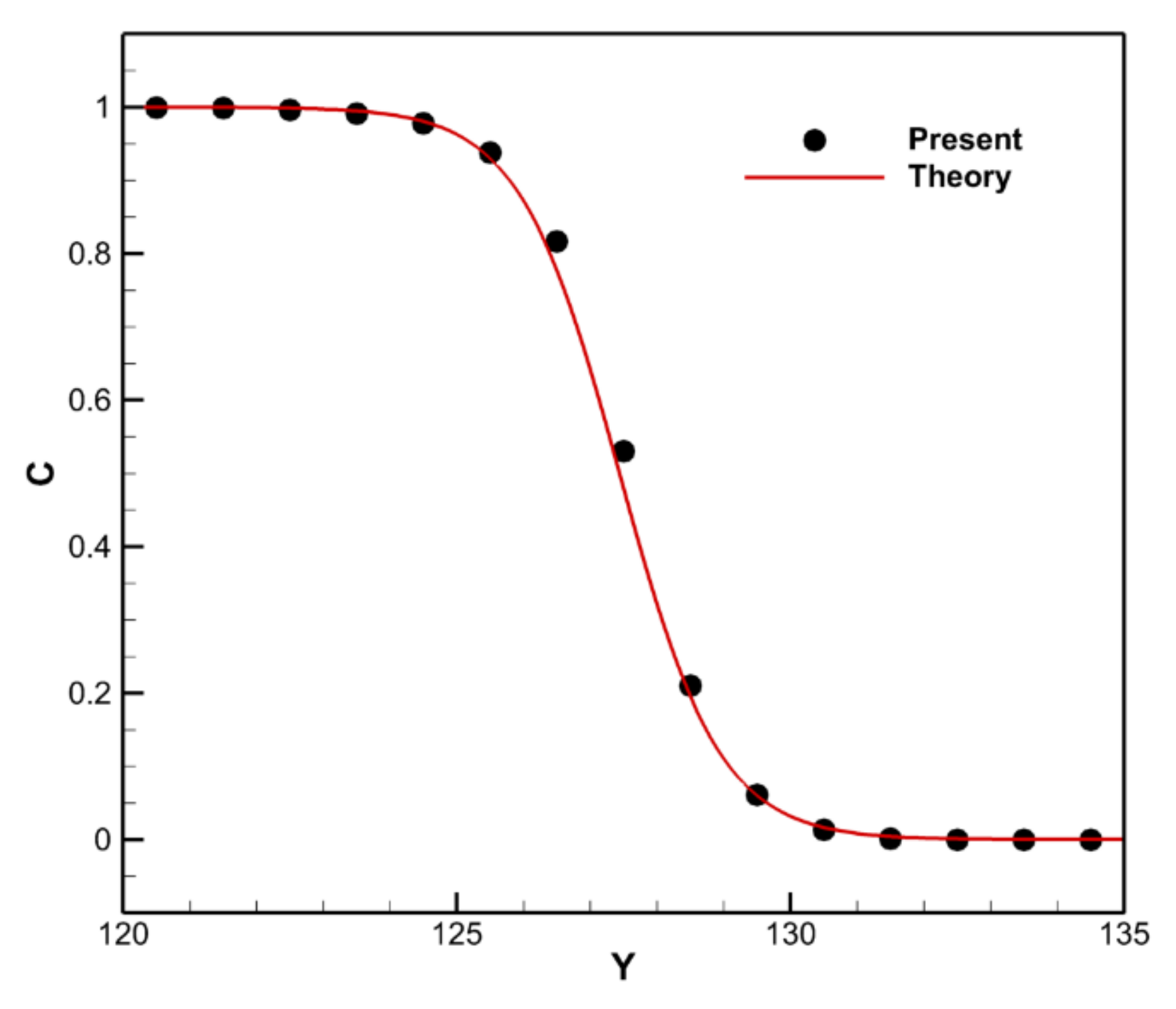
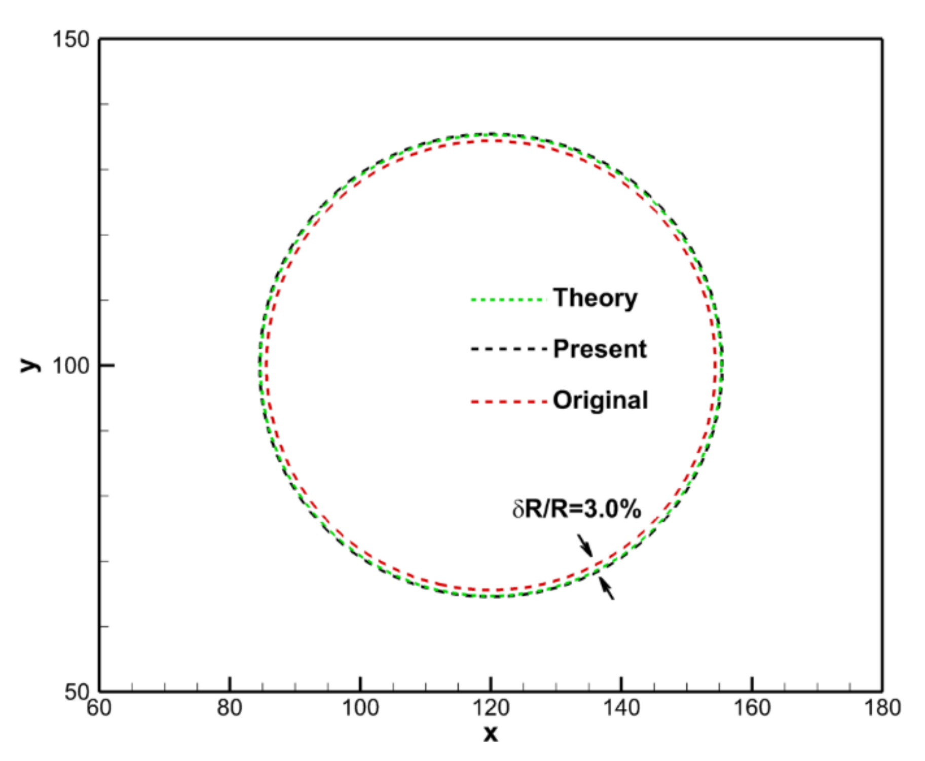
Figure 4 shows the pressure difference in and out of the bubble at $\sigma =0.001, 0.005$. It is obvious that the obtained results correspond with the prediction of the law. Figure 5 shows the variation in the mass for the whole bubble with the present method and the original DI approach for the case of $\sigma =0.005$, and Figure 6 shows the contrast of the final interface for the static bubble with $R=20$ at $\sigma =0.005$. It is clear that the present method conserved the fluid mass well. However, the bubble mass obtained with the original DI method decreased, and the speed at which the mass decreased obtained by the original method increased as the radius grew. Without the correction, up to 20% of the mass of the bubble could be lost. This characteristic agrees well with a previous study [37]. Figure 7 compares the profile of the order parameter C along the y-centerline of the flow domain and shows the results of interface shapes from the setting of the initial order parameter with different interface thicknesses $\xi =3,4,5,6$, obtained with the present interface correction method and the original DI method at $\sigma =0.001$. It should be noted that the surface force was calculated by setting the interface thickness $\xi =3$, which means that the final solution of the interface shape should be that described by Equation (6) with $\xi =3$, regardless of the initial conditions. As can be seen from Figure 7, the order parameter with different thicknesses from the original method cannot give an accurate theoretical value, while the present method was able to obtain correct interface shapes that agree well with theoretical solutions. This feature shows that, when the interface shape is compressed or diffused in the initial condition, the present method is able to adjust and, finally, maintain the interface shape acquired with the theory, which shows its effectiveness and reliability.

3.2. The Evolution of a Square Bubble

In nature, an irregular bubble immersed in another fluid changes to a circular one under the action of the surface tension without considering gravity. In this section, we study the deformation of a static square bubble. To mimic this process, the mesh size of $301\times 301$ was adopted for simulation. The natural boundary condition was applied to all walls. The following parameters were applied for simulations: ${\rho }_H=10$, ${\rho }_L=1$, ${\nu }_H={\nu }_L=0.002$, $\sigma$ as defined as 0.005, and $\xi =3$; in order to measure the size of the bubble, a parameter $R=D/2$ was set, where $D$ is the length of the side for the square bubble. Cases of R = 20, 40, and 60 were simulated. The parameters of the coefficient $k=k_1\mathrm{\Gamma }{\left(\frac{\mathrm{\Delta }x}{L}\right)}^2$ in Equation (11) were set as $k_1=1$ and $L=2R$.

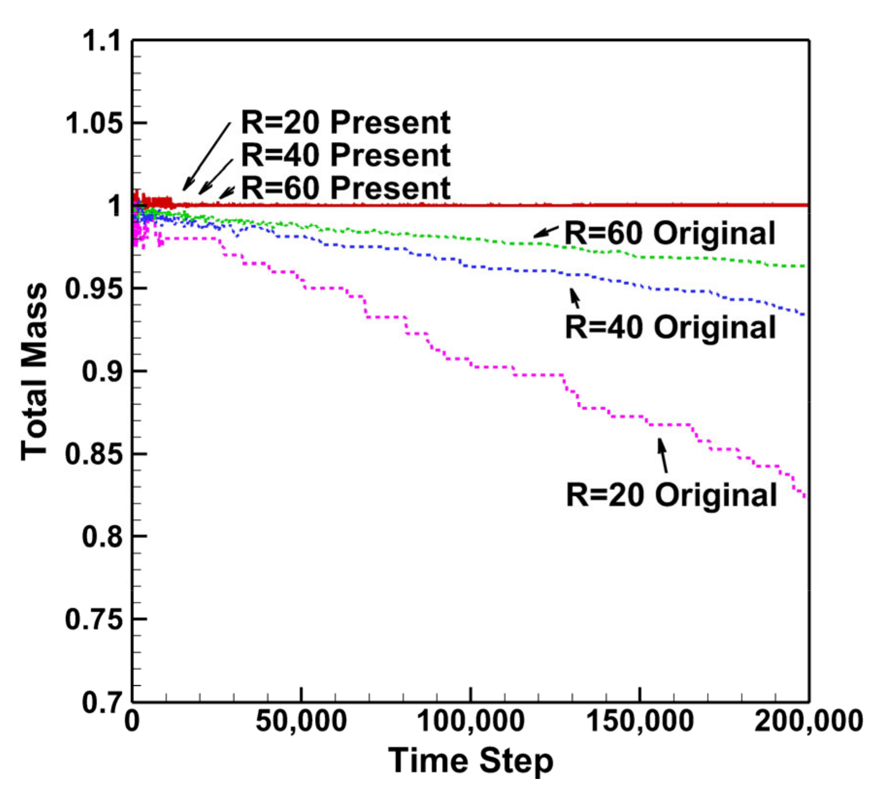
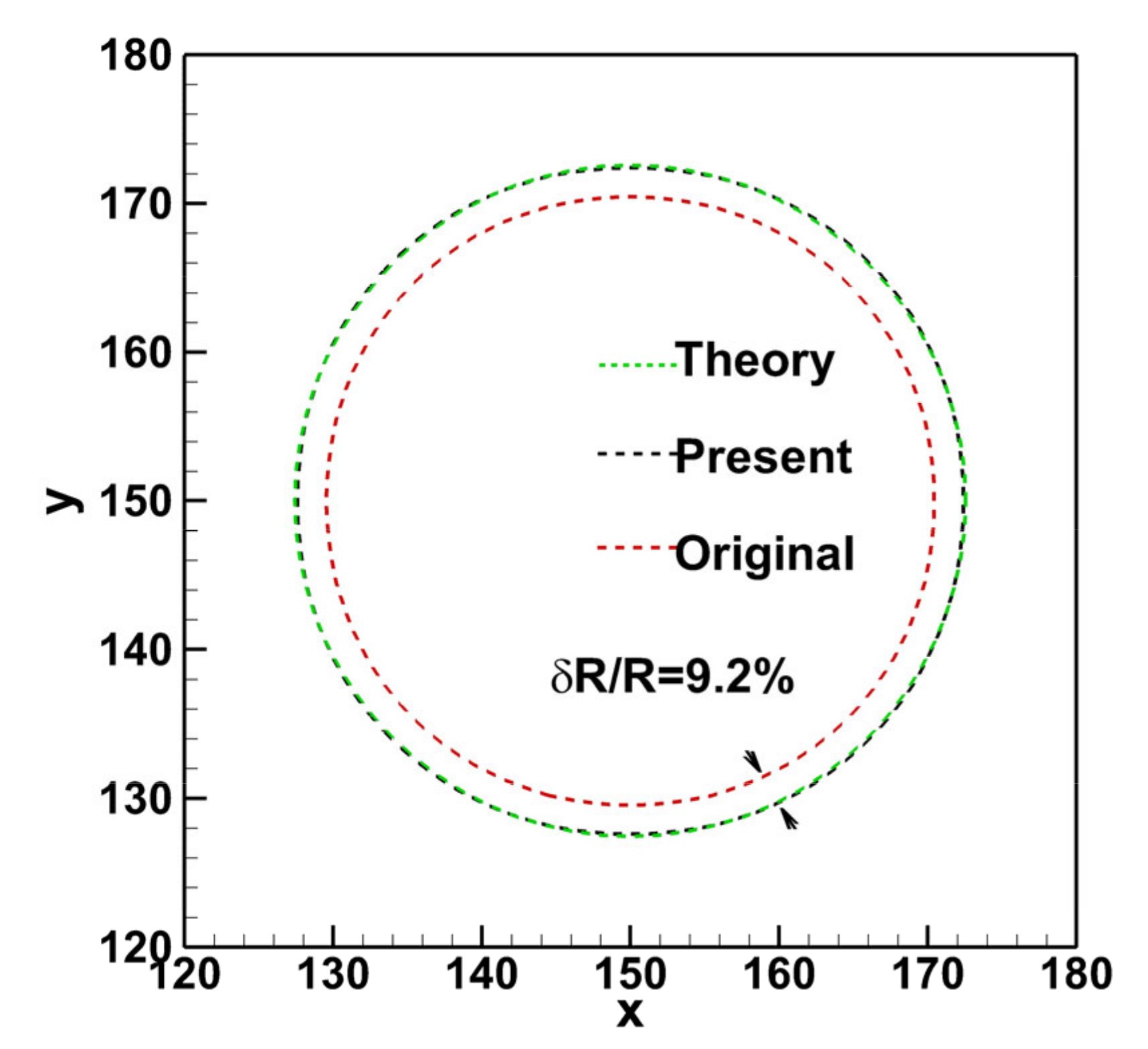
Figure 8 shows the variation in the mass for the square bubble obtained with the two methods with different radii for the case of $\sigma =0.005$. It is obvious that the present method had better behavior in mass conservation. In contrast, the mass obtained with the original method decreases and the mass loss increases as the radius grows, which is consistent with the previous results of verifying the Laplace law. Figure 9 shows the results for the final shape with the two methods and compares them with the theoretical solutions for $R=20$ at $\sigma =0.005$. For the original DI method, as shown in the Figure 9, the change of the radius is 9.2% lower than the value of 12.5% in Figure 6. Figure 10 shows the contour of the order parameter along the centerline in the y direction of the whole zone of $R=20$ obtained with the present method, which agrees well with the analytical solution. In Figure 11, the development of the interface for the bubble with $R=20$ from a square shape to a circular shape is shown. The four corners of the square bubble are shrunk and the shape turns into a circle with the surface tension. All the phenomena verify that the present method has good reliability for mass conservation and the capability of maintaining interfacial shapes.

3.3. Two Merging Bubbles

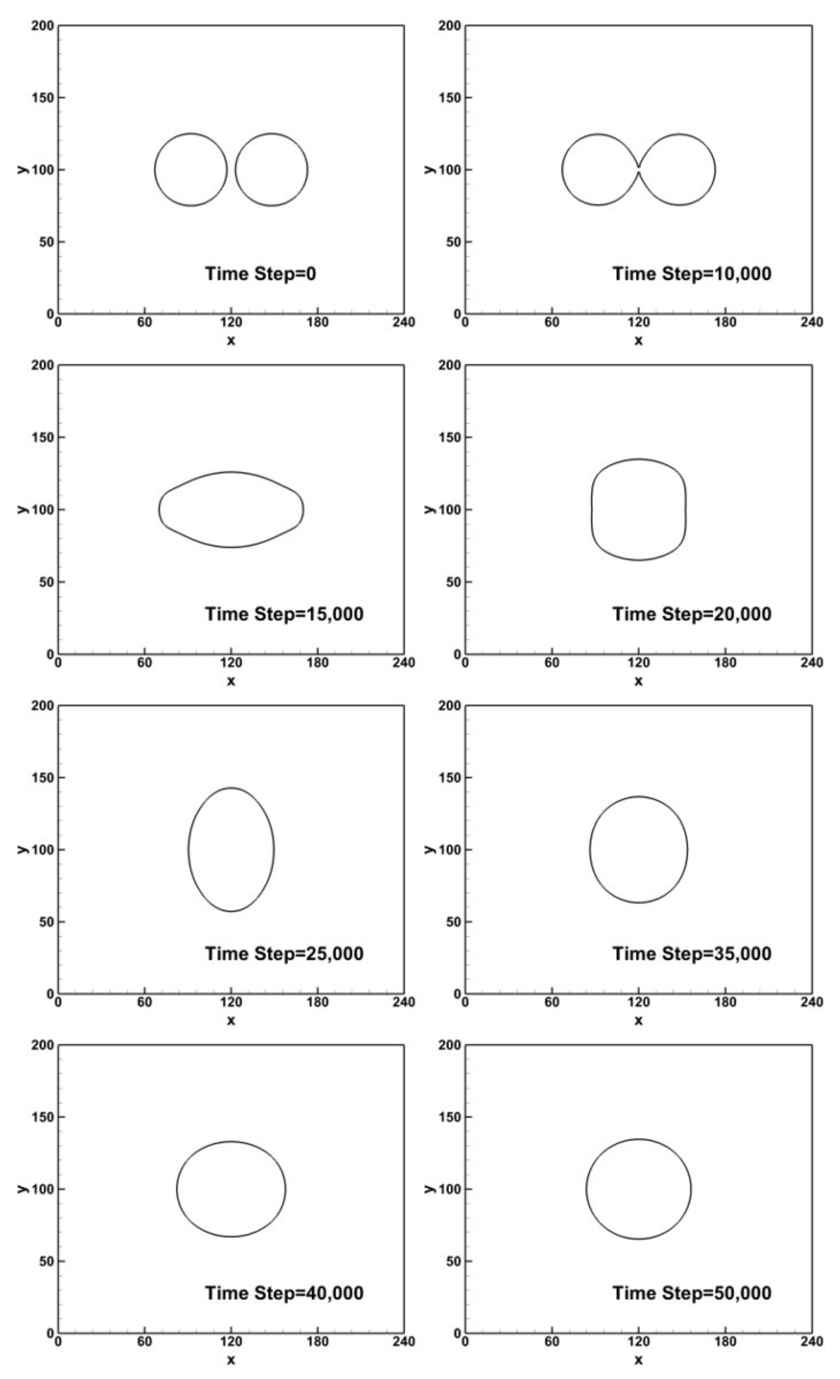
The merging of two bubbles is considered in this part to further validate the method that we have proposed. A previous study [11] found that, when the distance $d$ between interfaces of two bubbles is less than twice the interface thickness $2\xi$, the bubbles will merge under the action of the surface tension. To simulate this process, a mesh size of $241\times 201$ was adopted for the simulation. The natural boundary condition was applied to all walls. Initially, the two bubbles with radius $R=25$ were set at $\left(92,100\right)$ and $\left(148,100\right)$. There was a distance of $d=6$ between the interfaces of the two bubbles. The following parameters were adopted: ${\rho }_H=10$, ${\rho }_L=1$, ${\nu }_H={\nu }_L=0.002$, $\sigma =0.005$, and $\xi =4$. The parameters of the coefficient $k=k_1\mathrm{\Gamma }{\left(\frac{\mathrm{\Delta }x}{L}\right)}^2$ in Equation (11) were set as $k_1=1$ and $L=2R$. By calculating the parameters, it is obvious that the bubbles will merge.

Figure 12 shows the results for the final interface position obtained with the proposed method and with the original DI method and compares them with the theoretical solutions. It can be seen that the mass loss still exists with the calculation, while the result obtained with the present method is consistent with the theoretical solution. Figure 13 shows the development of the interface of two bubbles merging simulated with the proposed method at different times. It can be clearly observed that the two bubbles touch, merge, and produce a stable bubble. During the whole process, the interfacial shape is maintained well without seeing the non-physical phenomenon. The results indicate that the present method has good reliability in mass conservation and is effective in maintaining interfacial shapes.

3.4. Rayleigh–Taylor Instability

The Rayleigh–Taylor instability is of great importance for multiphase flow studies and thus it is studied in this section. The computational zone is a rectangular box of $\mathrm{\Omega }=\left[-d/2,d/2\right]\times \left[-2d,2d\right]$ ($d$ is the width of the box), where the heavier fluid is set in the upper location and the lighter fluid is set in the lower location. Initially, there is a small disturbance at the interface between the two fluids. The position disturbance function is $y\left(x\right)=0.1d cos\left(2\pi x/d\right)$ in the beginning. The periodic boundary condition was adopted at the left and right walls and the no-slip boundary condition was adopted at the top and bottom boundaries. The study is governed by two non-dimensional parameters: the Reynolds number and the Atwood number, $\mathrm{Re}=\frac{d\sqrt{gd}}{\nu }$ and $At=\frac{{\rho }_H-{\rho }_L}{{\rho }_H+{\rho }_L}$, where $g$ is the gravitational acceleration, ${\nu }_H={\nu }_L=\nu$. These parameters were set for the study: $d=200$, $\sqrt{gd}=0.01$, ${\rho }_L=1$, $\xi =3$, and $At=0.5$, and the conditions $Re=256$ and 3000 were studied. The parameters of the coefficient $k=k_1\mathrm{\Gamma }{\left(\frac{\mathrm{\Delta }x}{L}\right)}^2$ in Equation (11) were set as $L=d$ and $k_1=1$ or $k_1=10$ to observe the influence of the correlation coefficient.

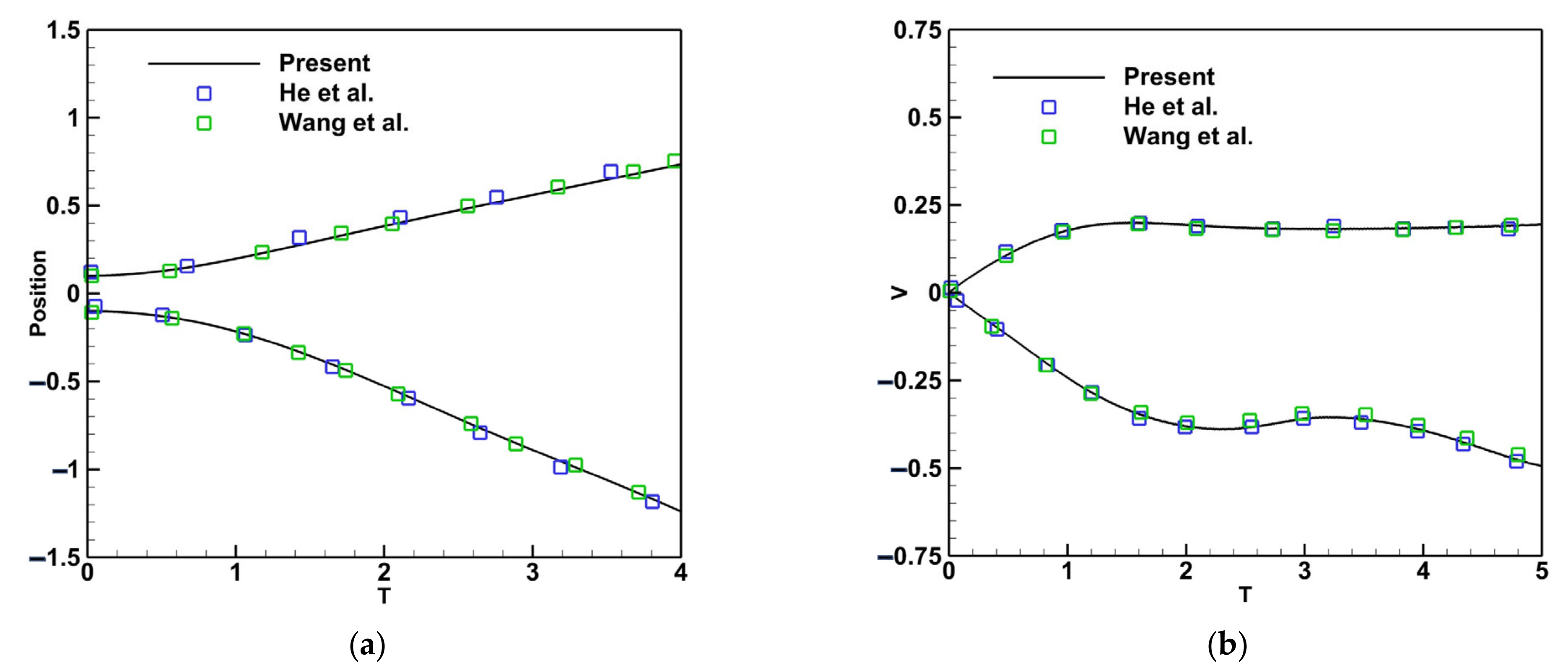
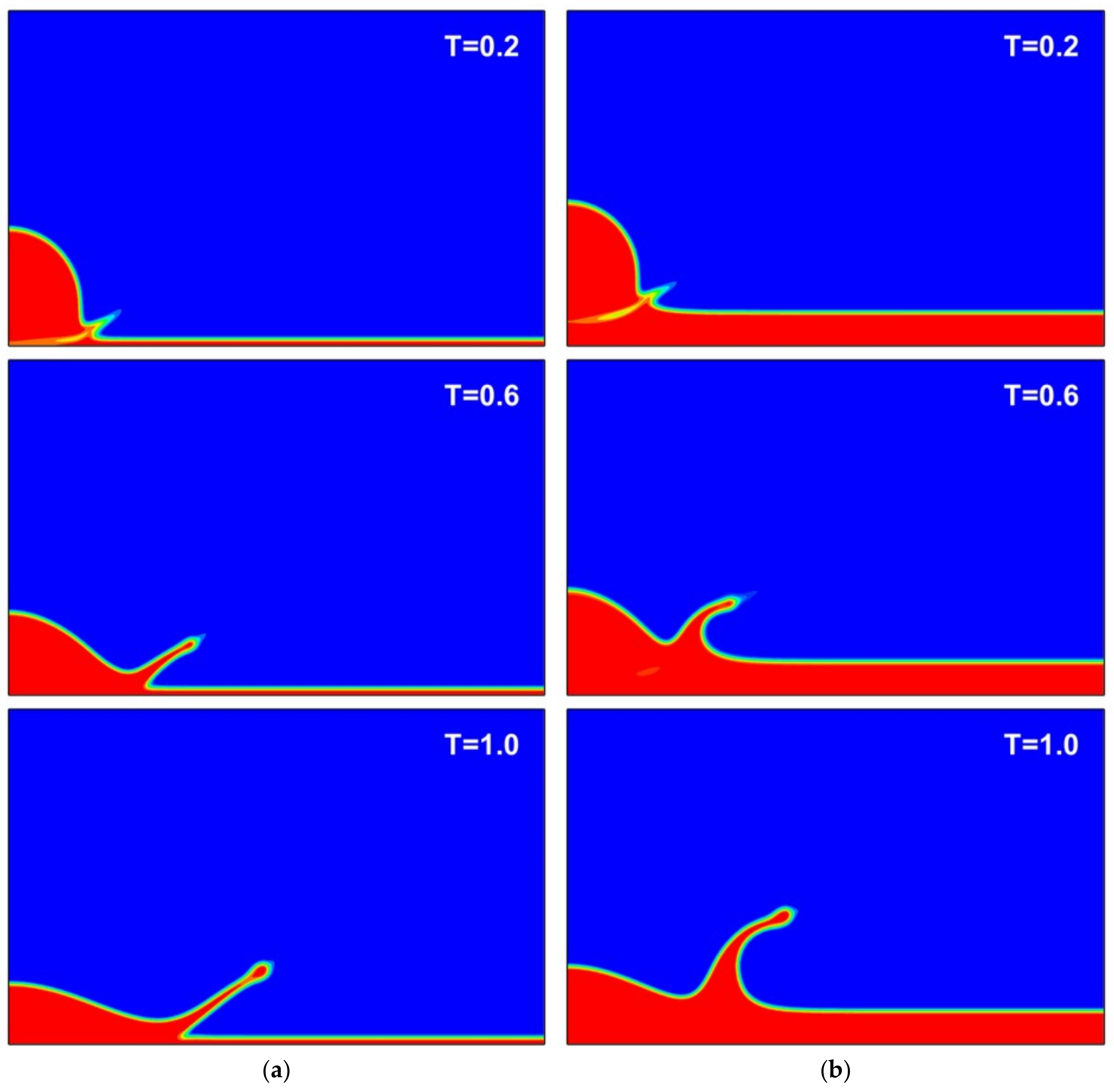
For the case of $Re=256$, we set $k_1=10$. Figure 14 compares the interface positions and the velocities of the rising bubble of light fluid and the falling spike of heavy fluid with the previous studies. They agree well with the references [10,22]. Figure 15 shows the evolution of the total mass of the lighter phase in the present method and the original DI method. The mass obtained with the original method is not stable compared with the present method.

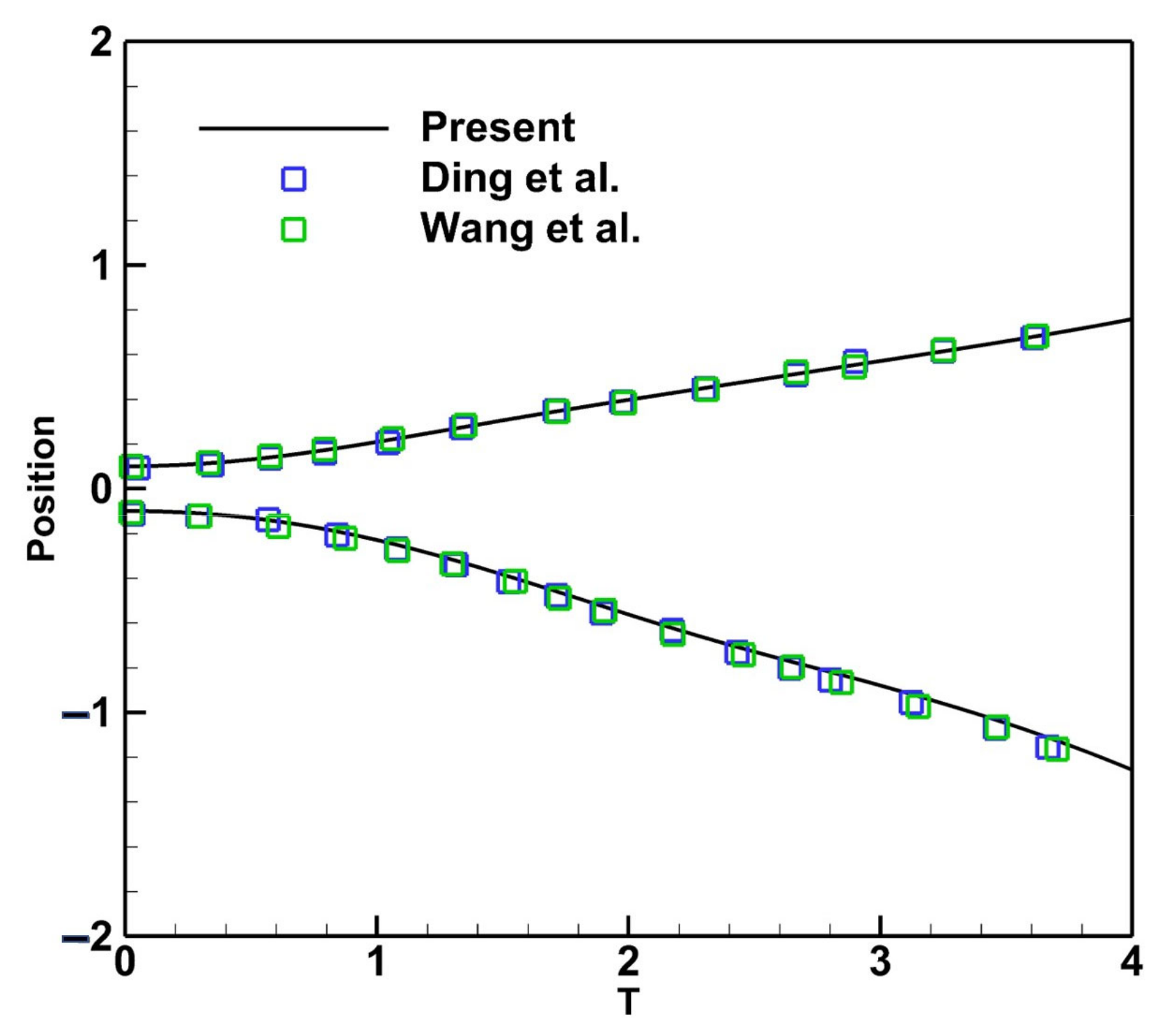
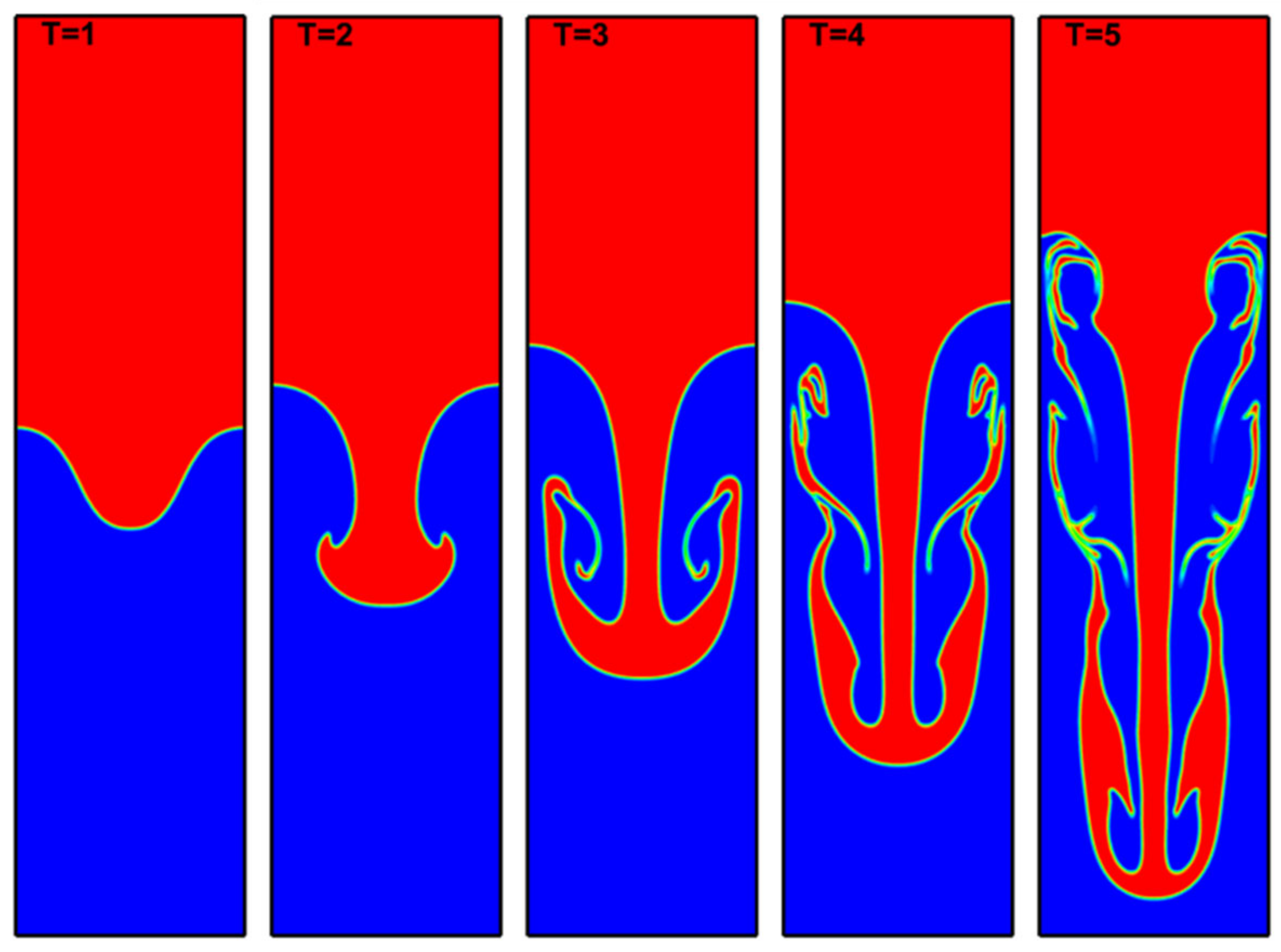
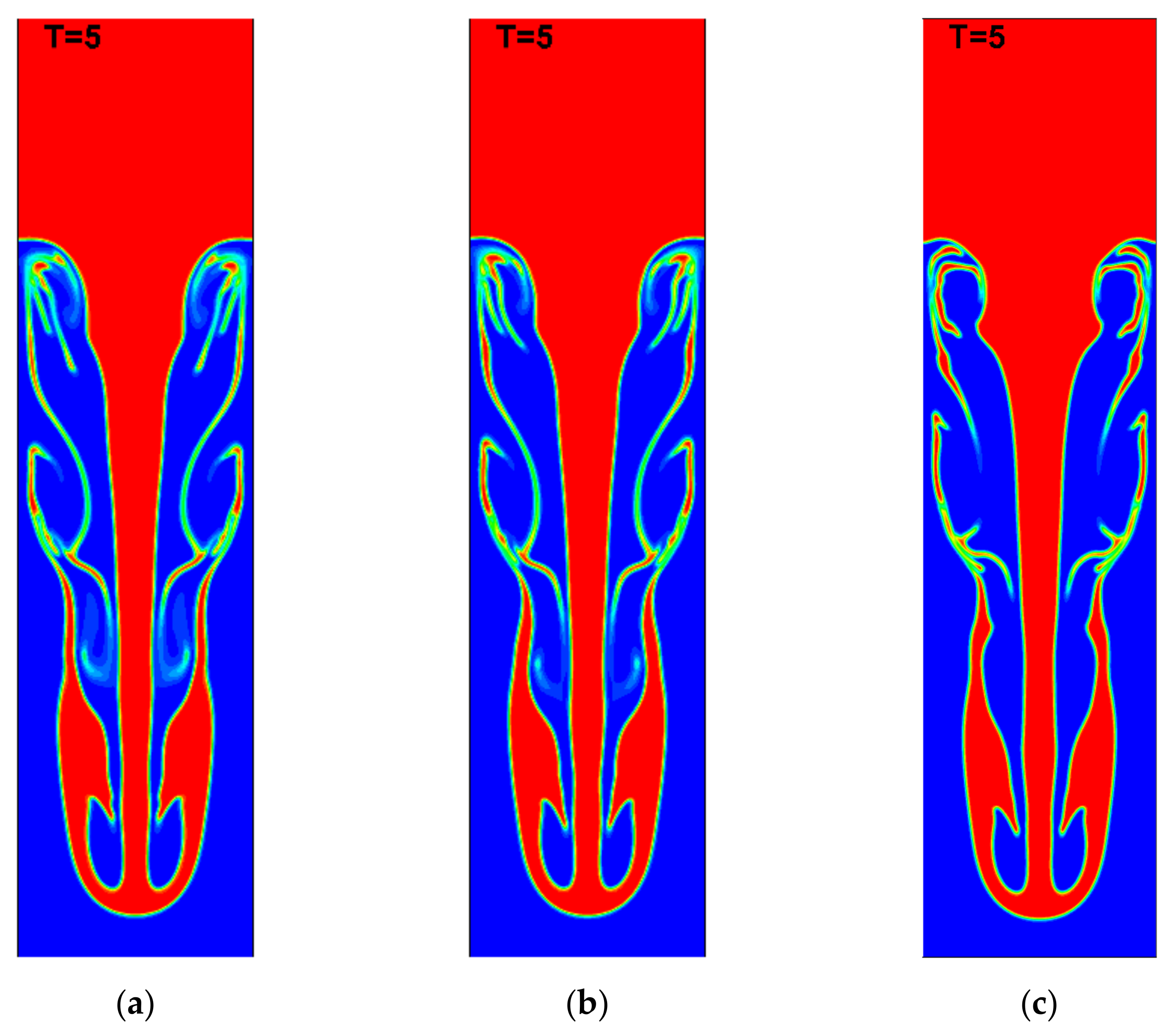
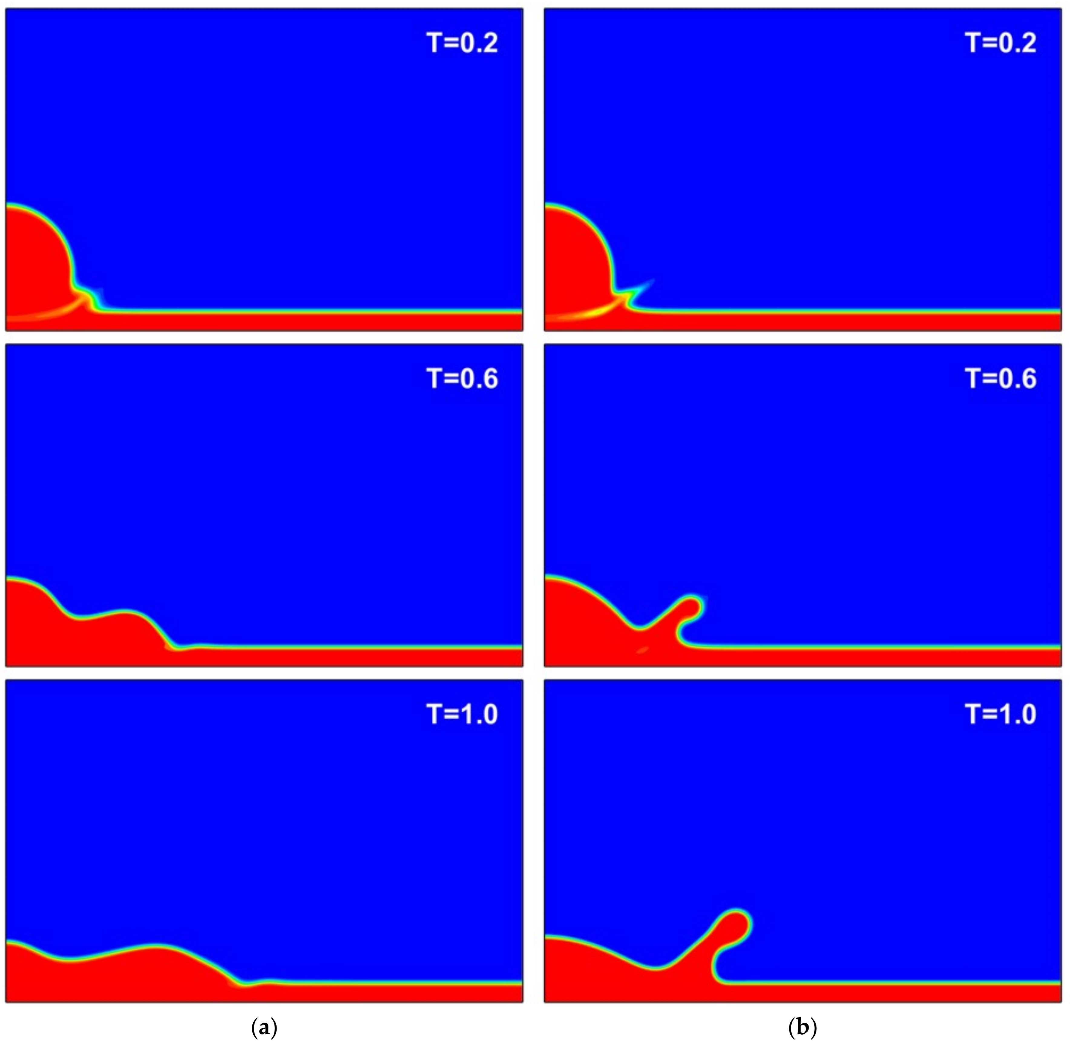
For the case of $Re=3000$, we set $k_1=1$ or $k_1=10$ to explore the influence of the correlation coefficient on the interface. First, we set $k_1=10$ and compared the interface positions with the previous studies [10,45], as shown in Figure 16. The present results agree well with the published data. Figure 17 shows the development of the interface for the Rayleigh–Taylor instability of $Re=3000$ with the present method at $k_1=10$. The production of the falling spike of the heavier fluid and the rising bubble of the lighter fluid can be clearly observed. At first, the heavier fluid close to the falling spike produces some small droplets, and then the small droplets break away from the spike. As time goes by, the droplets sloughed off will generate some smaller droplets and slough them off as before. The phenomena verify the Kelvin–Helmholtz instability. Finally, Figure 18 shows the interface shapes of the original method and the present method with $k_1=1$ and $k_1=10$ at $T=5$. For the interface shape obtained with the original DI method, the interfacial dispersion is quite strong. The interface of the droplet sloughed off from the heavy fluid is fuzzy. For the case of $k_1=1$, the interfacial dispersion is weaker than the original method. However, the phenomenon is not obvious, and the bands between the droplets can also be found. For the case of $k_1=10$, the interfacial dispersion is suppressed significantly. The interface shape is much clearer than those of the two other cases and the bands between the droplets almost disappear. It is illustrated that the coefficient of the correction term has a great influence on the interface and an appropriate coefficient determined by the flow parameters can suppress the interfacial dispersion well. In conclusion, it is obvious that the present approach has huge advantages in conserving mass and maintaining interfacial shapes compared with the original method.

3.5. Droplet Splashing on a Thin Film

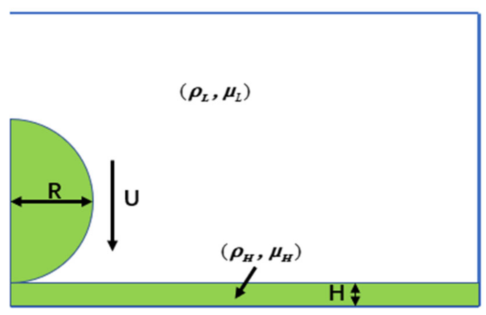
A droplet splashing on a liquid film is significant in studying multiphase flows, so we studied it to test the reliability of the proposed method for solving multiphase flows with large density ratios and high Reynolds numbers. The schematic diagram of the study is illustrated in Figure 19, where a droplet moves down with the velocity $U$ to a film without considering gravity. The heavier droplet is in an ambient lighter vapor field. The radius of the droplet is $R$ and the height of the film is $H$. The density and the dynamic viscosity of the liquid droplet and vapor are given respectively as $\left({\rho }_H,{\mu }_H\right)$ and $\left({\rho }_L,{\mu }_L\right)$. This problem can be governed by two non-dimensional parameters: the Reynolds number $Re=\frac{2RU}{{\nu }_H}$ and the Weber number $We=\frac{2{\rho }_H{U}^{2}R}{\sigma }$, where $\sigma$ is the surface tension. The computational zone only occupies half of the flow field due to the symmetric flow. To mimic this process, a mesh size of $401\times 251$ was adopted. The natural boundary condition was adopted on the top wall and the right wall, while the no-slip boundary condition was adopted on the bottom wall and the symmetric boundary condition was adopted on the left wall. The flow parameters were set as follows: $R=50$, $H=15$, $U=0.02$, ${\rho }_H=1$, ${\rho }_L=0.001$, ${\nu }_L=0.05$, $\xi =4$, and $We=150$, while $Re$ was defined as 100, 400, 800, and 2000. As for the coefficient $k$ in Equation (11), $k$ was defined as $k=k_1{\left(\frac{\mathrm{\Delta }x}{L}\right)}^2$ and, in this section, $k_1=0.4$ and $L=2R$.

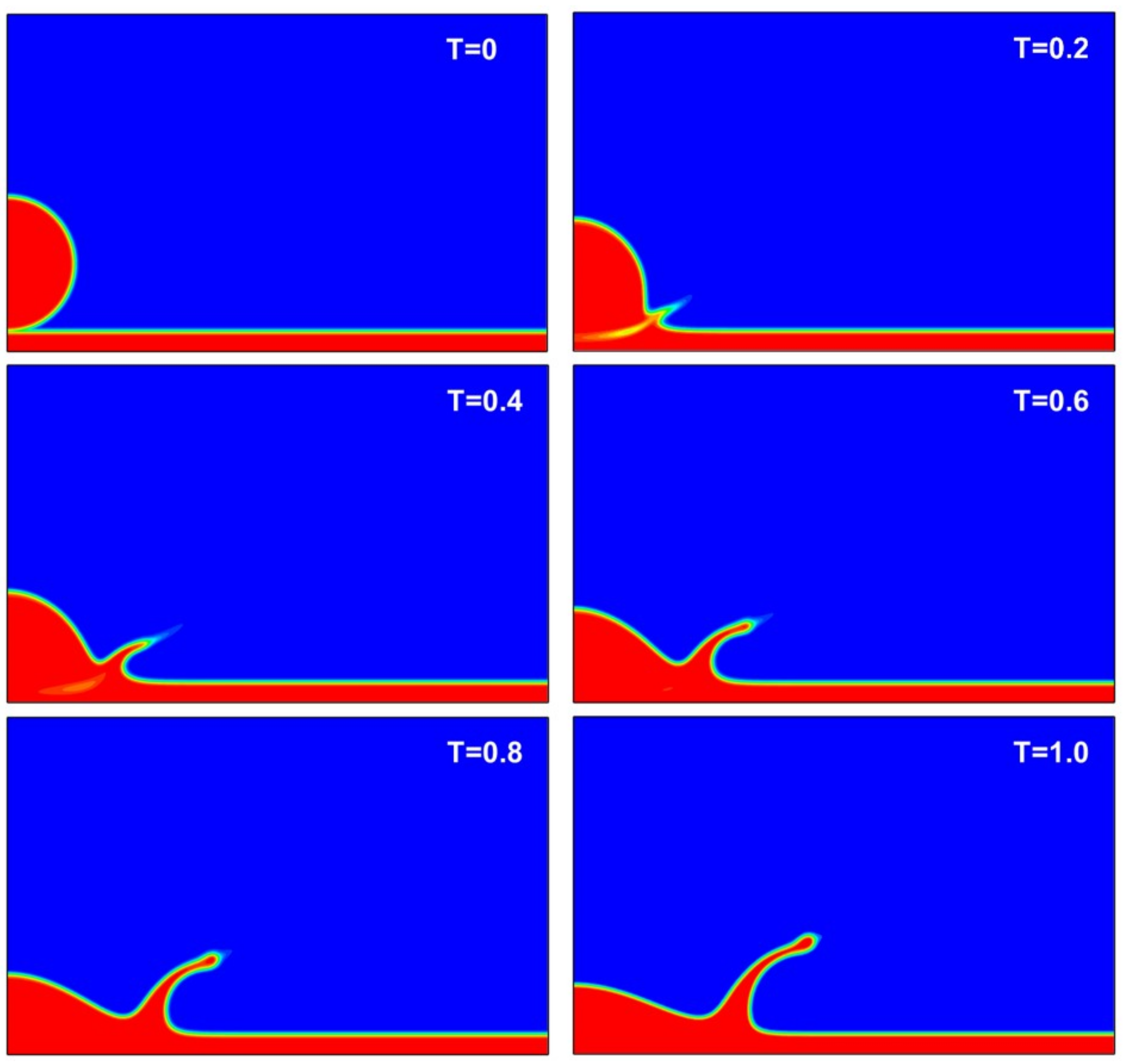
Figure 20 shows the development of the interface from T = 0–1 at $Re=800$ and $We=150$ with the present method. It can be clearly observed that a peak appears from the location between the droplet and the film, and then a small droplet appears on the top of the peak due to the surface tension. A clear liquid finger can be found after T = 0.6. In this condition, the finger is strong enough such that the breakup of the splashing liquid cannot occur.

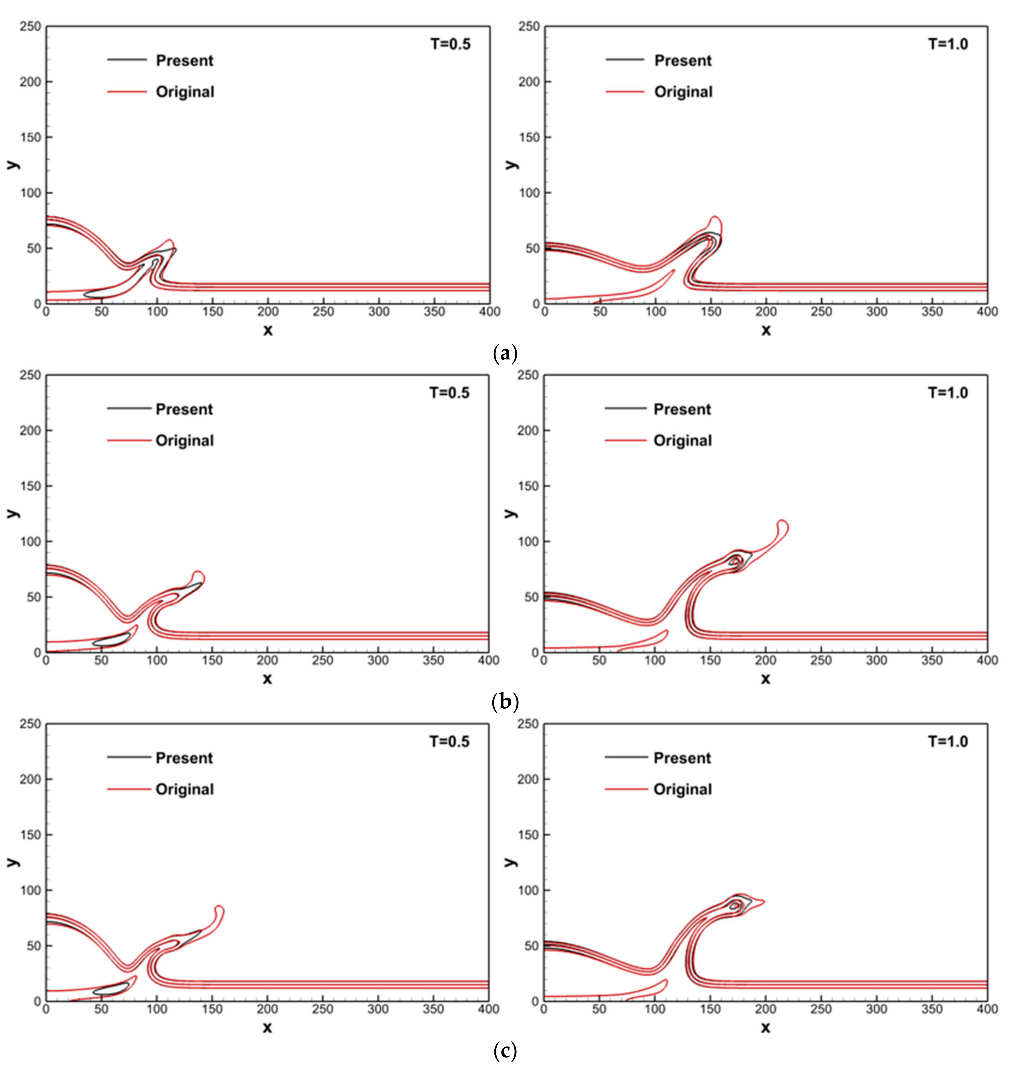
Figure 21 shows a comparison of the interface shape at different Reynolds numbers with the present approach and the original DI approach. The contour lines of the order parameter are divided into 0.05, 0.5, and 0.95 to observe the interface zone of the multiphase flow. We chose the results for $Re=100$, 800, and 2000 to examine whether the present method has a great influence on the interface zone compared with the original DI method. In the condition where $Re=100$, the interface thickness obtained with the present approach is smaller than the thickness from the original approach. With the Reynolds number increasing, the difference in the interface thickness is larger. The interface thickness of $Re=800$ and 2000 with the present method is much thinner, especially with the prominence of the liquid, which reflects the fact that the present method shows good improvement in the interface zone. It is proved that the present method has wonderful applicability in maintaining interfacial shapes for simulating the flows of high Reynolds numbers.

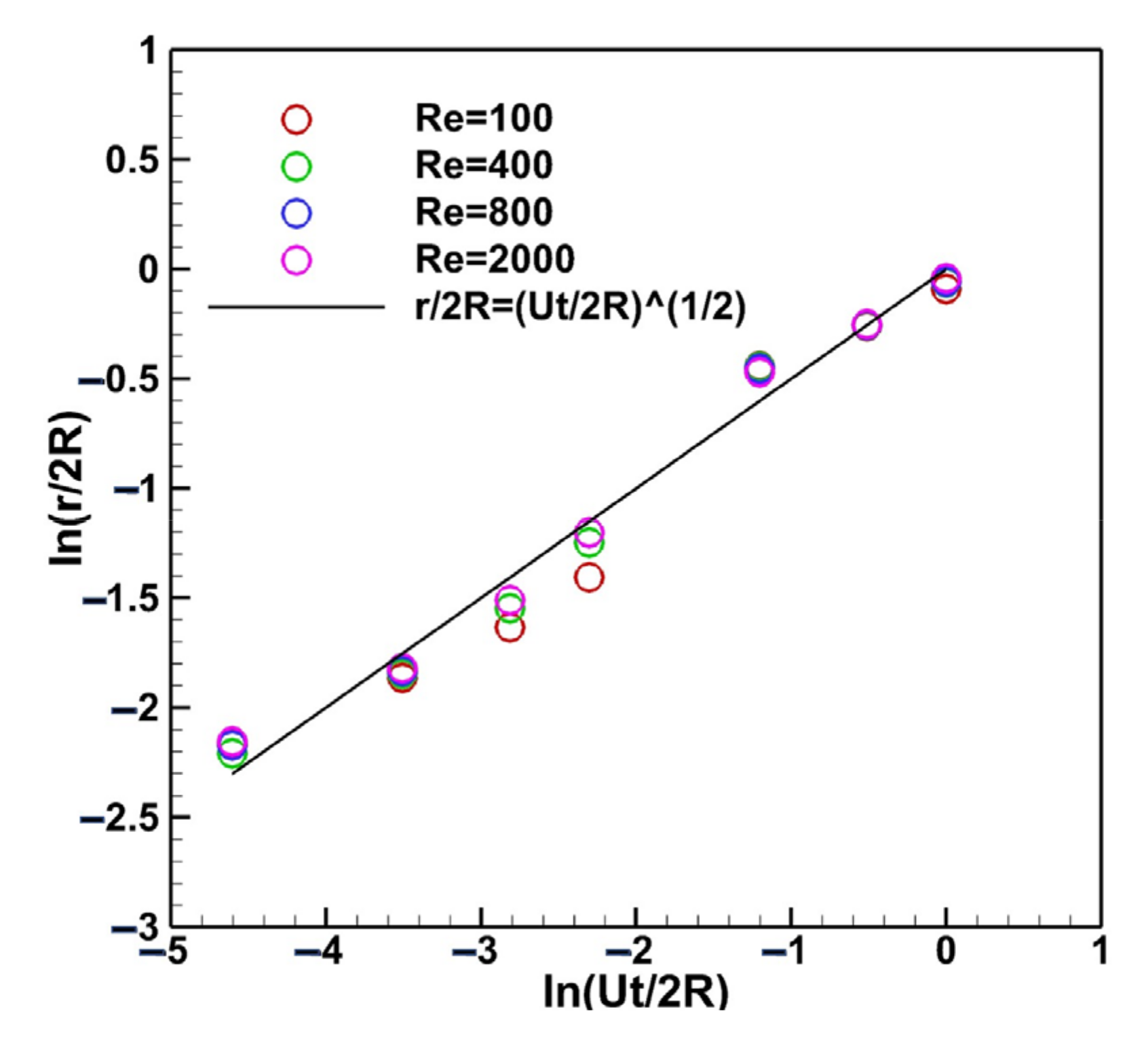
To examine the correctness of the results, the spread radius was measured. A previous study [46] shows that, when splashing occurs, the spread radius obeys a power law $r/(2R)\approx \sqrt{Ut/\left(2R\right)}$. Figure 22 shows the comparison of the present impact radius with different Reynolds numbers. It can be seen that the present results conform to the prediction of the law.

On this basis, we changed the initial conditions of the droplet splashing to determine the influence of the height of the thin film and the Weber number. We chose the condition of $Re=800$, $We=150$, and $H=15$ as the benchmark. All other simulations were transformed from this.

Figure 23 shows the evolution of the interface shapes for the droplet splashing on a thin film at $Re=800$, $We=150$, and $H=5$ or $H=25$ with the present approach. According to Figure 23a, the height of the liquid film is pretty small and, after the droplet splashes, the shape of the sputtering liquid between the droplet and the film is straighter than the others shown in Figure 20 and Figure 23b. It can be seen that the angle of $H=5$ between the sputtering liquid and the film is smaller than the angles of $H=15$ and $H=25$ at T = 0.6 and T = 1.0. As time goes by, the clearer circle droplet appears from the top of the sputtering liquid. As for Figure 23b, the liquid deformation of the droplet and the film is similar to the condition of $H=15$ in Figure 20; however, the angle between the sputtering liquid and the film with $H=25$ is a little larger than the one with $H=15$. In conclusion, the angle is bigger when the height is larger with other parameters unchanged. The film prevents the liquid from splashing after impacting, and the height of the film has a great effect when the height is pretty small. It can be speculated that the resistance and the kinetic energy loss will be larger during splashing when the film is thicker. However, the influence of the resistance and the kinetic energy loss is limited in a range such that the angle will remain ultimately unchanged even if the height is larger, according to Figure 20 and Figure 23. For the same droplet, the simulation results for the interface shape will be almost the same when the height of the film is large enough.

Figure 24 shows the development of the fluid interface with $Re=800$, $H=15$, and $We=10$ or $We=50$ with the present method. According to Figure 24a, for the case of $We=10$, the peak of the liquid is almost absent at T = 0.2, and then, at T = 0.6, the liquid forms a hump instead of a peak. The liquid forms a wave rather than a clear liquid finger, as in Figure 20 and Figure 24b. In this condition, the fluid movement is greatly affected by the surface tension, which limits the droplet splashing on the film. As for Figure 24b with $We=50$, the peak of the liquid appears at T = 0.2; however, at T = 0.6, the shape of the liquid finger from the location impacted is shorter and thicker compared with the condition where $We=150$. At T = 1.0, the shape of the liquid finger is fatter and the height of the splashing liquid is lower than the condition where $We=150$. Differently from the small droplet at the top of the splashing liquid with $We=150$ at T = 1.0, the droplet is larger and has a tighter link with the liquid film. In general, the surface tension prevents the liquid from splashing outward, and it is difficult for the small droplet to come into being after the impact when the surface tension is relatively large. The kinetic energy loss is larger when the Weber number is larger, such that the height of the splashing droplet is lower and the small droplet cannot arise or break away from the liquid due to the surface tension. By simulating the multiphase flows of different conditions, the reliability of the present method was validated. The improved numerical method has great potential for use in practical applications involving multiphase flows with large density ratios.

4. Conclusions

Due to convection and diffusion, the shape as well as the thickness of a fluid interface cannot be maintained for numerical simulations of multiphase flows. Furthermore, mass conservation cannot be guaranteed in the DI method because of physical and numerical diffusion when solving the C–H equation. In order to resolve these problems, an interface-corrected DI method with an improved MLBFS for solving incompressible multiphase flows was proposed. An interface correction term was introduced into the DI model by applying the Hamilton–Jacobi equation. This term only took effect around the interfaces between different phases. The fluxes were reconstructed by applying the particle distribution functions both before and after collisions. A local switch function was also introduced to automatically adjust the contributions of these distribution functions to the fluxes. A mass correction term was also introduced into the DI model to maintain mass conservation.

The accuracy and capability of the proposed DI method were validated by simulating the Laplace law, the evolution of a square bubble, two bubbles merging, the Rayleigh–Taylor instability, and a droplet splashing on a thin film at a density ratio of 1000 with Reynolds numbers in a range from 100 to 2000. Then, the droplet splashing problem, along with other conditions, was explored on the previous basis and good results were obtained. By adding the correction terms to the interface zone, the mass conservation property of the fluids was found to be pretty good and the results for the interface shape were better than before. The interface shape and thickness with the proposed method were maintained better compared with the results from the original DI method. Moreover, fluxes could be evaluated according to the characteristics of the local multiphase flows. On the basis of the present results, the proposed method has high potential for effectively solving complex multiphase flows by maintaining the interface shape and mass conservation simultaneously.

References

- Hirt, C.W.; Nichols, B.D. Volume of fluid (VOF) method for the dynamics of free boundaries. J. Comput. Phys. 1981, 39, 201–225. [Google Scholar] [CrossRef]
- Garoosi, F.; Merabtene, T.; Mahdi, T.-F. Numerical simulation of merging of two rising bubbles with different densities and diameters using an enhanced Volume-Of-Fluid (VOF) model. Ocean Eng. 2022, 247, 110711. [Google Scholar] [CrossRef]
- Mulder, W.; Osher, S.; Sethian, J.A. Computing interface motion in compressible gas dynamics. J. Comput. Phys. 1992, 100, 209–228. [Google Scholar] [CrossRef]
- Sussman, M.; Smereka, P.; Osher, S. A Level Set Approach for Computing Solutions to Incompressible Two-Phase Flow. J. Comput. Phys. 1994, 114, 146–159. [Google Scholar] [CrossRef]
- Tryggvason, G.; Bunner, B.; Esmaeeli, A.; Juric, D.; Al-Rawahi, N.; Tauber, W.; Han, J.; Nas, S.; Jan, Y.J. A Front-Tracking Method for the Computations of Multiphase Flow. J. Comput. Phys. 2001, 169, 708–759. [Google Scholar] [CrossRef]
- Bayareh, M.; Mortazavi, S. Three-dimensional numerical simulation of drops suspended in simple shear flow at finite Reynolds numbers. Int. J. Multiph. Flow 2011, 37, 1315–1330. [Google Scholar] [CrossRef]
- Bayareh, M.; Doostmohammadi, A.; Dabiri, S.; Ardekani, A.M. On the rising motion of a drop in stratified fluids. Phys. Fluids 2013, 25, 023029. [Google Scholar] [CrossRef]
- Zhang, T.J.; Wu, J.; Lin, X.J. An improved diffuse interface method for three-dimensional multiphase flows with complex interface deformation. Int. J. Numer. Methods Fluids 2020, 92, 976–991. [Google Scholar] [CrossRef]
- Yue, P.T.; Feng, J.J.; Liu, C.; Shen, J. A diffuse-interface method for simulating two-phase flows of complex fluids. J. Fluid Mech. 2004, 515, 293–317. [Google Scholar] [CrossRef]
- Wang, Y.; Shu, C.; Huang, H.B.; Teo, C.J. Multiphase lattice Boltzmann flux solver for incompressible multiphase flows with large density ratio. J. Comput. Phys. 2015, 280, 404–423. [Google Scholar] [CrossRef]
- Zheng, H.W.; Shu, C.; Chew, Y.T. A lattice Boltzmann model for multiphase flows with large density ratio. J. Comput. Phys. 2006, 218, 353–371. [Google Scholar] [CrossRef]
- Gelissen, E.J.; van der Geld, C.W.M.; Baltussen, M.W.; Kuerten, J.G.M. Modeling of droplet impact on a heated solid surface with a diffuse interface model. Int. J. Multiph. Flow 2020, 123, 103173. [Google Scholar] [CrossRef]
- Gurtin, M.E.; Polignone, D.; Vinals, J. Two-phase binary fluids and immiscible fluids described by an order parameter. Math. Models Methods Appl. Sci. 1996, 6, 815–831. [Google Scholar] [CrossRef]
- Boyer, F. A theoretical and numerical model for the study of incompressible mixture flows. Comput. Fluids 2002, 31, 41–68. [Google Scholar] [CrossRef]
- D’Humières, D.; Lallemand, P. Lattice gas automata for fluid mechanics. Phys. A (Amst. Neth.) 1986, 140, 326–335. [Google Scholar] [CrossRef]
- Huang, H.; Zheng, H.; Lu, X.Y.; Shu, C. An evaluation of a 3D free-energy-based lattice Boltzmann model for multiphase flows with large density ratio. Int. J. Numer. Methods Fluids 2010, 63, 1193–1207. [Google Scholar] [CrossRef]
- Reis, T. A lattice Boltzmann formulation of the one-fluid model for multiphase flow. J. Comput. Phys. 2022, 453, 110962. [Google Scholar] [CrossRef]
- Li, X.; Dong, Z.Q.; Li, Y.; Wang, L.P.; Niu, X.D.; Yamaguchi, H.; Li, D.C.; Yu, P. A fractional-step lattice Boltzmann method for multiphase flows with complex interfacial behavior and large density contrast. Int. J. Multiph. Flow 2022, 149, 103982. [Google Scholar] [CrossRef]
- Gunstensen, A.K.; Rothman, D.H.; Zaleski, S.; Zanetti, G. Lattice Boltzmann model of immiscible fluids. Phys. Rev. A 1991, 43, 4320–4327. [Google Scholar] [CrossRef]
- Shan, X.; Chen, H. Lattice Boltzmann model for simulating flows with multiple phases and components. Phys. Rev. E 1993, 47, 1815–1819. [Google Scholar] [CrossRef] [Green Version]
- Swift, M.R.; Orlandini, E.; Osborn, W.R.; Yeomans, J.M. Lattice Boltzmann simulations of liquid-gas and binary fluid systems. Phys. Rev. E: Stat. Phys., Plasmas, Fluids, Relat. Interdiscip. Top. 1996, 54, 5041–5052. [Google Scholar] [CrossRef] [PubMed]
- He, X.; Chen, S.; Zhang, R. A Lattice Boltzmann Scheme for Incompressible Multiphase Flow and Its Application in Simulation of Rayleigh-Taylor Instability. J. Comput. Phys. 1999, 152, 642–663. [Google Scholar] [CrossRef]
- Inamuro, T.; Ogata, T.; Tajima, S.; Konishi, N. A lattice Boltzmann method for incompressible two-phase flows with large density differences. J. Comput. Phys. 2004, 198, 628–644. [Google Scholar] [CrossRef]
- Lee, T.; Lin, C.-L. A stable discretization of the lattice Boltzmann equation for simulation of incompressible two-phase flows at high density ratio. J. Comput. Phys. 2005, 206, 16–47. [Google Scholar] [CrossRef]
- Hu, Y.; Li, D.C.; Niu, X.D.; Shu, S. A diffuse interface lattice Boltzmann model for thermocapillary flows with large density ratio and thermophysical parameters contrasts. Int. J. Heat Mass Transfer. 2019, 138, 809–824. [Google Scholar] [CrossRef]
- Li, Q.; Niu, X.; Lu, Z.; Li, Y.; Khan, A.; Yu, Z. An improved single-relaxation-time multiphase lattice boltzmann model for multiphase flows with large density ratios and high reynolds numbers. Adv. Appl. Mech. 2020, 13, 426–454. [Google Scholar]
- Yuan, H.Z.; Wang, Y.; Shu, C. An adaptive mesh refinement-multiphase lattice Boltzmann flux solver for simulation of complex binary fluid flows. Phys. Fluids 2017, 29, 123604. [Google Scholar] [CrossRef]
- Yang, L.M.; Shu, C.; Chen, Z.; Hou, G.X.; Wang, Y. An improved multiphase lattice Boltzmann flux solver for the simulation of incompressible flow with large density ratio and complex interface. Phys. Fluids 2021, 33, 033306. [Google Scholar] [CrossRef]
- Yang, L.M.; Shu, C.; Chen, Z.; Wang, Y.; Hou, G.X. A simplified lattice Boltzmann flux solver for multiphase flows with large density ratio. Int. J. Numer. Methods Fluids 2021, 93, 1895–1912. [Google Scholar] [CrossRef]
- Van der Sman, R.G.M.; van der Graaf, S. Emulsion droplet deformation and breakup with Lattice Boltzmann model. Comput. Phys. Commun. 2008, 178, 492–504. [Google Scholar] [CrossRef]
- Zheng, L.; Lee, T.; Guo, Z.; Rumschitzki, D. Shrinkage of bubbles and drops in the lattice Boltzmann equation method for nonideal gases. Phys. Rev. E 2014, 89, 033302. [Google Scholar] [CrossRef] [PubMed]
- Aland, S.; Voigt, A. Benchmark computations of diffuse interface models for two-dimensional bubble dynamics. Int. J. Numer. Methods Fluids 2012, 69, 747–761. [Google Scholar] [CrossRef]
- Ding, H.; Yuan, C.J. On the diffuse interface method using a dual-resolution Cartesian grid. J. Comput. Phys. 2014, 273, 243–254. [Google Scholar] [CrossRef]
- Chao, J.; Mei, R.; Singh, R.; Shyy, W. A filter-based, mass-conserving lattice Boltzmann method for immiscible multiphase flows. Int. J. Numer. Methods Fluids 2011, 66, 622–647. [Google Scholar] [CrossRef]
- Wang, Y.; Shu, C.; Shao, J.Y.; Wu, J.; Niu, X.D. A mass-conserved diffuse interface method and its application for incompressible multiphase flows with large density ratio. J. Comput. Phys. 2015, 290, 336–351. [Google Scholar] [CrossRef]
- Yang, L.; Shu, C.; Yu, Y.; Wang, Y.; Hou, G. A mass-conserved fractional step axisymmetric lattice Boltzmann flux solver for incompressible multiphase flows with large density ratio. Phys. Fluids 2020, 32, 103308. [Google Scholar] [CrossRef]
- Li, Y.B.; Choi, J.I.; Kim, J. A phase-field fluid modeling and computation with interfacial profile correction term. Commun Nonlinear Sci. 2016, 30, 84–100. [Google Scholar] [CrossRef]
- Zhang, Y.J.; Ye, W.J. A Flux-Corrected Phase-Field Method for Surface Diffusion. Commun. Comput. Phys. 2017, 22, 422–440. [Google Scholar] [CrossRef]
- Soligo, G.; Roccon, A.; Soldati, A. Mass-conservation-improved phase field methods for turbulent multiphase flow simulation. Acta Mech. 2019, 230, 683–696. [Google Scholar] [CrossRef]
- Wang, Y.; Shu, C.; Yang, L.M.; Yuan, H.Z. On the re-initialization of fluid interfaces in diffuse interface method. Comput. Fluids 2018, 166, 209–217. [Google Scholar] [CrossRef]
- Zhang, T.W.; Wu, J.; Lin, X.J. An interface-compressed diffuse interface method and its application for multiphase flows. Phys. Fluids 2019, 31, 122102. [Google Scholar]
- Wang, Y.; Shu, C.; Yang, L.M. An improved multiphase lattice Boltzmann flux solver for three-dimensional flows with large density ratio and high Reynolds number. J. Comput. Phys. 2015, 302, 41–58. [Google Scholar] [CrossRef]
- Xu, K. Gas-kinetic schemes for unsteady compressible flow simulations. In 29th Computational Fluid Dynamics; Annual Lecture Series; Von Karman Institute for Fluid Dynamics: Rhode-Saint-Genese, Belgium, 1998. [Google Scholar]
- Xu, K. A Gas-Kinetic BGK Scheme for the Navier-Stokes Equations and Its Connection with Artificial Dissipation and Godunov Method. J. Comput. Phys. 2001, 171, 289–335. [Google Scholar] [CrossRef]
- Ding, H.; Spelt, P.D.M.; Shu, C. Diffuse interface model for incompressible two-phase flows with large density ratios. J. Comput. Phys. 2007, 226, 2078–2095. [Google Scholar] [CrossRef]
- Josserand, C.; Zaleski, S. Droplet splashing on a thin liquid film. Phys. Fluids 2003, 15, 1650–1657. [Google Scholar] [CrossRef]
Figure 1.
Illustration of the structure for two-phase flows.
Figure 2.
The D2Q9 lattice velocity model.
Figure 3.
Illustration of the flux evaluation at cell surfaces.
Figure 4.
Pressure difference inside and outside the bubble at σ = 0.001 and 0.005.
Figure 5.
Variation in the mass for the bubble at σ = 0.005.
Figure 6.
The final interface shapes for the static bubble of R = 20 at σ = 0.005.
Figure 7.
The order parameter along the y-centerline with different initial interface thicknesses at σ = 0.001: (a) present method, (b) original method.
Figure 8.
Variation in the mass for the whole bubble at σ = 0.005.
Figure 9.
Contrast of the final interface for the bubble with R = 20 at σ = 0.005.
Figure 10.
Contrast of the contour for the order parameter along the y-centerline with the analytical solution for σ = 0.005 at R = 20.
Figure 11.
Development of the interface for the square bubble of R = 20.
Figure 12.
Comparison of the final interfaces for the merging bubbles.
Figure 13.
Development of the interface for bubbles merging.
Figure 14.
Interface positions and velocities of the bubble and spike for the Rayleigh–Taylor instability at Re = 256 compared with references [10,22]: (a) interface positions, (b) interface velocities.
Figure 15.
Variation in the mass for the lighter fluid at Re = 256.
Figure 16.
Interface positions of the bubble and spike for the Rayleigh–Taylor instability of Re = 3000 compared with references [10,45].
Figure 17.
Development of the interface for the Rayleigh–Taylor instability of Re = 3000 with the present approach ().
Figure 18.
Interface shapes for Rayleigh–Taylor instability of Re = 3000 (T = 5): (a) original method, (b) present method with , (c) present method with .
Figure 19.
Illustration of the droplet splashing on a thin film.
Figure 20.
Development of the interface at Re = 800 and We = 150 with the present method.
Figure 21.
Comparison of the interface shapes of different Reynolds number with two methods; the three contour lines from up to down: 0.05, 0.5, 0.95. (a) Re = 100, (b) Re = 800, (c) Re = 2000.
Figure 22.
Comparison of the predicted spread radius with different Reynolds numbers.
Figure 23.
Development of the interface with Re = 800 and We = 150 with the present method: (a) H = 5, (b) H = 25.
Figure 24.
Development of the interface with Re = 800 and H = 15 with the present method: (a) We = 10, (b) We = 50.
Publisher’s Note: MDPI stays neutral with regard to jurisdictional claims in published maps and institutional affiliations. |
© 2022 by the authors. Licensee MDPI, Basel, Switzerland. This article is an open access article distributed under the terms and conditions of the Creative Commons Attribution (CC BY) license (https://creativecommons.org/licenses/by/4.0/).
Share and Cite
MDPI and ACS Style
Guo, Y.; Wang, Y.; Hao, Q.; Wang, T. An Interface-Corrected Diffuse Interface Model for Incompressible Multiphase Flows with Large Density Ratios. Appl. Sci. 2022, 12, 9337. https://doi.org/10.3390/app12189337
AMA Style
Guo Y, Wang Y, Hao Q, Wang T. An Interface-Corrected Diffuse Interface Model for Incompressible Multiphase Flows with Large Density Ratios. Applied Sciences. 2022; 12(18):9337. https://doi.org/10.3390/app12189337
Chicago/Turabian StyleGuo, Yuhao, Yan Wang, Qiqi Hao, and Tongguang Wang. 2022. "An Interface-Corrected Diffuse Interface Model for Incompressible Multiphase Flows with Large Density Ratios" Applied Sciences 12, no. 18: 9337. https://doi.org/10.3390/app12189337
Note that from the first issue of 2016, this journal uses article numbers instead of page numbers. See further details here.