Article

A Comparative Study of Control Methods for X3D Quadrotor Feedback Trajectory Control

by
Tanzeela Shakeel
1,†,
Jehangir Arshad
2,*,†,
Mujtaba Hussain Jaffery
2,
Ateeq Ur Rehman
3,
Elsayed Tag Eldin
4,*,
Nivin A. Ghamry
5 and
Muhammad Shafiq
6,*
1
Department of Computer Science, University of Management and Technology, Lahore 54000, Pakistan
2
Department of Electrical & Computer Engineering, COMSATS University Islamabad Lahore Campus, Lahore 54000, Pakistan
3
Department of Electrical Engineering, Government College University, Lahore 54000, Pakistan
4
Faculty of Engineering and Technology, Future University in Egypt, New Cairo 11835, Egypt
5
Faculty of Computers and Artificial intelligence, Cairo University, Giza 3750010, Egypt
6
Department of Information and Communication Engineering, Yeungnam University, Gyeongsan 38541, Korea
*
Authors to whom correspondence should be addressed.
These authors contributed equally to this work.
Appl. Sci. 2022, 12(18), 9254; https://doi.org/10.3390/app12189254
Submission received: 4 August 2022 / Revised: 5 September 2022 / Accepted: 8 September 2022 / Published: 15 September 2022
(This article belongs to the Special Issue Trajectory Analysis, Positioning and Control of Mobile Robots)

Abstract

:
Unmanned aerial vehicles (UAVs), particularly quadrotor, have seen steady growth in use over the last several decades. The quadrotor is an under-actuated nonlinear system with few actuators in comparison to the degree of freedom (DOF); hence, stabilizing its attitude and positions is a significant challenge. Furthermore, the inclusion of nonlinear dynamic factors and uncertainties makes controlling its maneuverability more challenging. The purpose of this research is to design, implement, and evaluate the effectiveness of linear and nonlinear control methods for controlling an X3D quadrotor’s intended translation position and rotation angles while hovering. The dynamics of the X3D quadrotor model were implemented in Simulink. Two linear controllers, linear quadratic regulator (LQR) and proportional integral derivate (PID), and two nonlinear controllers, fuzzy controller (FC) and model reference adaptive PID Controller (MRAPC) employing the MIT rule, were devised and implemented for the response analysis. In the MATLAB Simulink Environment, the transient performance of nonlinear and linear controllers for an X3D quadrotor is examined in terms of settling time, rising time, peak time, delay time, and overshoot. Simulation results suggest that the LQR control approach is better because of its robustness and comparatively superior performance characteristics to other controllers, particularly nonlinear controllers, listed at the same operating point, as overshoot is 0.0% and other factors are minimal for the x3D quadrotor. In addition, the LQR controller is intuitive and simple to implement. In this research, all control approaches were verified to provide adequate feedback for quadrotor stability.

1. Introduction

Unmanned aerial vehicles (UAVs) have recently acquired a great deal of interest for military and civil research applications when a human operator is too risky and time-consuming. Quadrotors have attracted the interest of scientists in the fields of robotics, automation, and aviation. A quadrotor is a rotorcraft with a simple nonlinear construction for vertical take-off and landing (VTOL). It is a system with four actuator inputs that are under actuated [1]. It features six degrees of freedom, with three translation positions: longitudinal (x-axis), lateral (y-axis), and height (z-axis), as well as three rotational states ( r o l l   ϕ   , p i t c h   θ   a n d   y a w   ψ ) . The thrust of the four rotors controls these output states. The thrust of the four rotors regulates these output states. Due to its fundamental dynamic nature, it offers a great maneuverability advantage. It has a good hovering ability and a quick response for tracking [2]. It is widely used in both outdoor and indoor situations for research and monitoring. High-performance quadrotor control in intense and maneuverable flight is a challenging problem due to the complex nature of the dynamic model, severe coupling, and nonlinear characteristics. Scientists may use the control of quadrotors for testing and evaluating novel concepts in a range of disciplines, including flight control theory, navigation, and real-time systems.
Many researchers from all around the globe have detailed various methods for operating quadrotor UAVs, to the extent of developing an effective stabilizing and navigation system based on the standard control input. A PID controller is extensively used in many industrial applications because of its simplicity and ease of implementation, on the other hand, the LQR controller provides better performance concerning certain measures of performance; fuzzy controller and adaptive PID controller are also extensively implemented for nonlinear systems. Many investigations have been performed on the application of PID, LQR, fuzzy, state feedback, and other control methods to quadrotor UAVs as a plant, but there has been relatively little study on the comparison of linear and nonlinear control methods. The study in [3] proposed a method for simulating and establishing parameters for a quadcopter to analyze and improve the performance of this system and its stability. The system was mounted on a structure that could be freely moved along a vertical axis. The computer received real-time data from sensors and measuring devices. The paper [4] proposed a comparison of nonlinear and linear control methods for quadrotor systems. In this paper [5], a comparison of PID and LQR control techniques is provided. Both controllers provide appropriate feedback for quadrotor stability, according to this study. For the quadrotor’s flip operation, Byung-Yoon Lee compares the performance of three distinct types of attitude control systems [6]; PID, sliding mode and open-loop controllers are all used in his article to develop quadrotor attitude controllers. PID control is one of the most often used control strategies [1], [7] along with back-stepping [8,9], nonlinear H control [10], Kalman filter [11], and so on. Other control methodologies, such as fuzzy control systems, are also investigated and applied to a quadrotor, as discussed in [12,13]. In the research in [14,15], the implementation, testation, validation, authentication, and comparison of LQR, PID, and state feedback controllers have been performed on an X3D Quadrotor in NI LabVIEW simulation. The application of sub-super-stochastic matrices to bipartite tracking control in sign networks is presented in [16]. The research [17] represented an innovative decentralized control strategy for the Cucker–Smale model to analyze the leader–follower flocking behavior on networks that encompass both cooperative and rival relationships between agents.
The research [18] addressed the PID and LQR controller implementation for the Qball X4 trajectory tracking. Simulations and experiments were conducted to compare the performance of the developed control strategies. A mathematical model was developed in the research paper [18] to simulate the behavior of a quadrotor with four motors driven by PID using a simple approach. In the study [19], feedback linearization and the LQR controller were proposed to stabilize the quadrotor attitude in the trajectory. A gain-scheduling fuzzy controller for quadrotor position and height control was proposed in the research [19]. The study [20] compared and implemented three controllers into an actual quadrotor in real-time, including PID, LQR, and backstepping. The research [21] offered three robust procedures for controlling a quadrotor in a predetermined trajectory based on the MIT rule and sliding-mode methods. A variety of commonly used quadrotor controllers were described in the previous study. With their algorithms, many control techniques have their strengths and limitations. As a result, the quadrotor’s applications and performance determine the appropriate controller. The strengths and limitations of several controllers for controlling quadrotor systems are presented in Table 1.
The primary motivation of this research is to show the experimental results of well-known and recently developed theoretical studies in the field of modern control system design and analysis for the quadrotor system. One of the most significant properties of control systems analysis is stability. Control systems must meet specified criteria for the system under investigation to operate as desired in both transient and steady-state response values that are as close to the desired value as possible. Therefore, the research presents the development and comparison of the quadrotor control system. The quadrotor plant is initially linearized for hover flight before the linear control approaches are implemented. This research compares the performance of linear and nonlinear control techniques, taking into consideration the restricted onboard computer resources. Because of the constraints imposed by nonlinearity factors and external disturbances, the primary goal is to maintain the translation position’s stability, attitude, and altitude of an x3D quadrotor. The key contribution of the proposed research is to develop control systems for x3D quadrotors that will allow them to control the translation position ( x , y , z ) while stabilizing its attitude angles ( r o l l   ϕ   , p i t c h   θ   a n d   y a w   ψ ) by forcing the position ( x , y , z ) and yaw ( ψ ) to track their respect to reference inputs while keeping the roll ( ϕ ) and pitch ( θ ) angles negligible [21]. The desired parameters, such as rise time, settling time, peak time, and maximum percent overshoot, and steady-state errors are analyzed in the MATLAB Simulink environment for the x3D quadrotor. As a result, the suggested solutions are more practical and feasible. The significant contributions of this research are as follows:
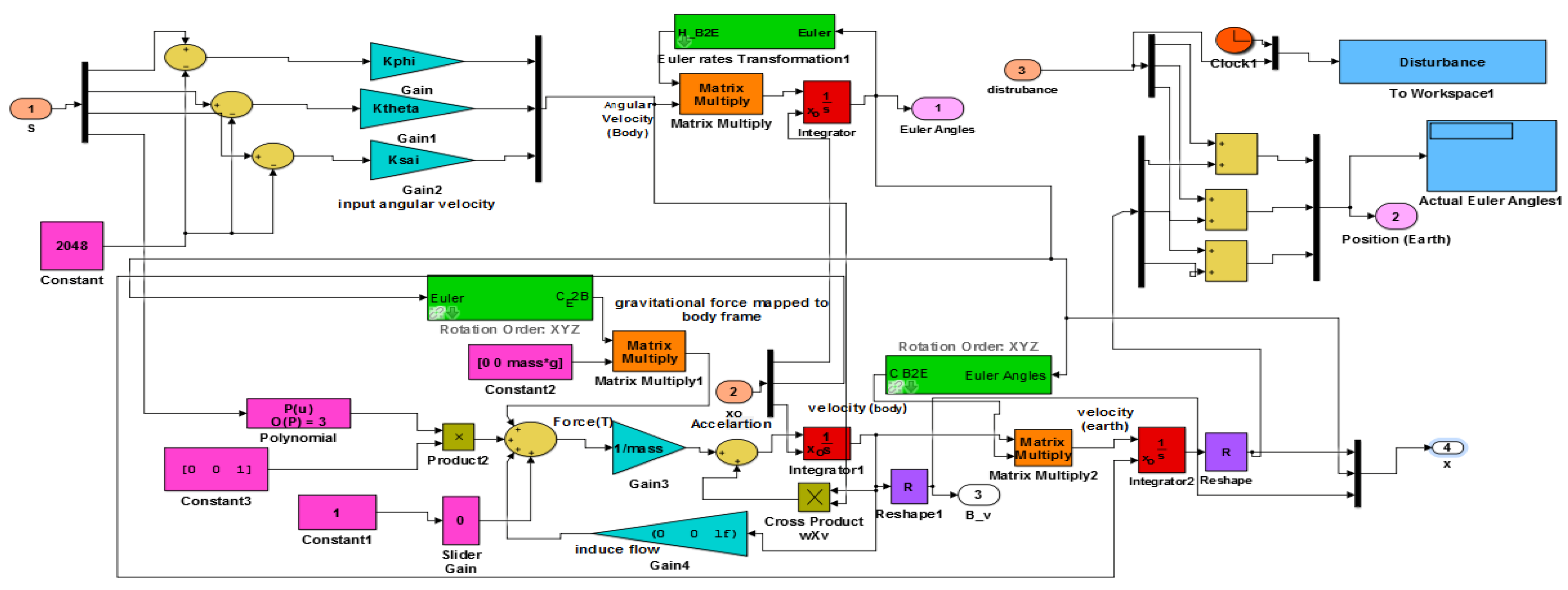
  • SIMULINK simulation of nonlinear X3D quadrotor model to validate control approaches.
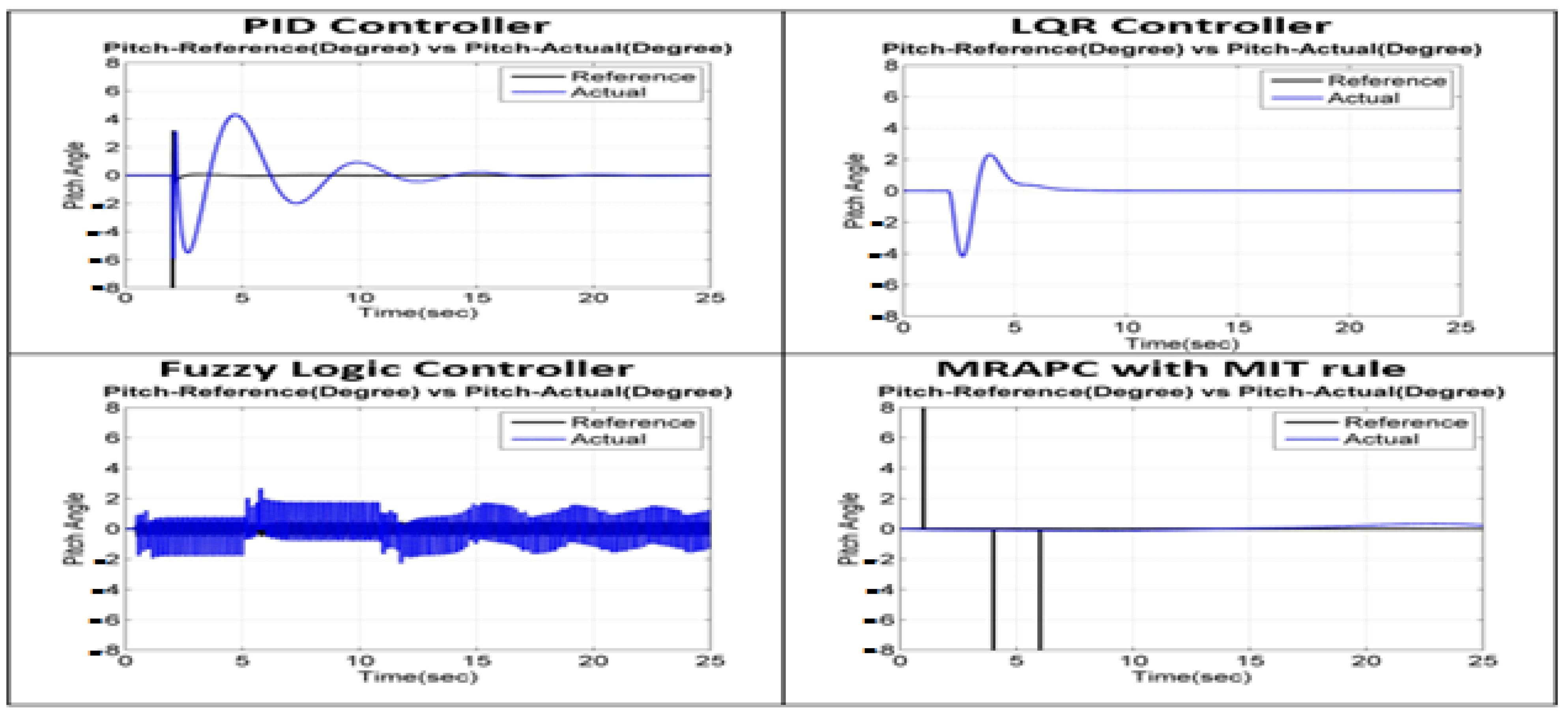
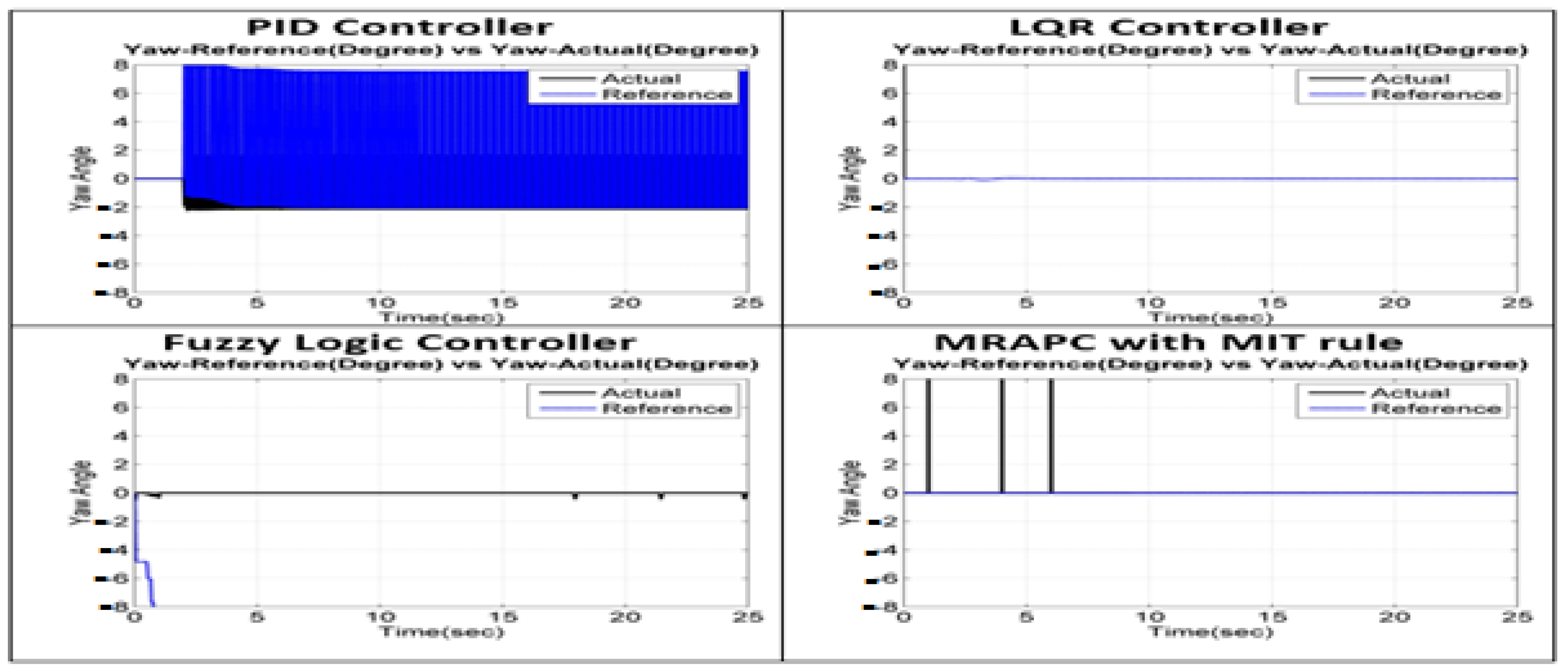
  • Two linear control systems are implemented: the conventional PID and the LQR control system.
  • Two nonlinear control systems are implemented: fuzzy control and model reference adaptive PID controller (MRAPC) using MIT rules.
  • Performance comparison of all controllers for quadrotor trajectory tracking based on transient response. The proposed controllers’ performance is anticipated to be better in the presence of parameter uncertainty and external disturbances.
The following is the format of this paper: The mathematical model of an X3D quadrotor is presented in Section 2. The quadrotor’s control methods are discussed in Section 3. The study and comparison of the aforementioned control strategies for an X3D quadrotor are presented in Section 4. The conclusion is found in Section 5.

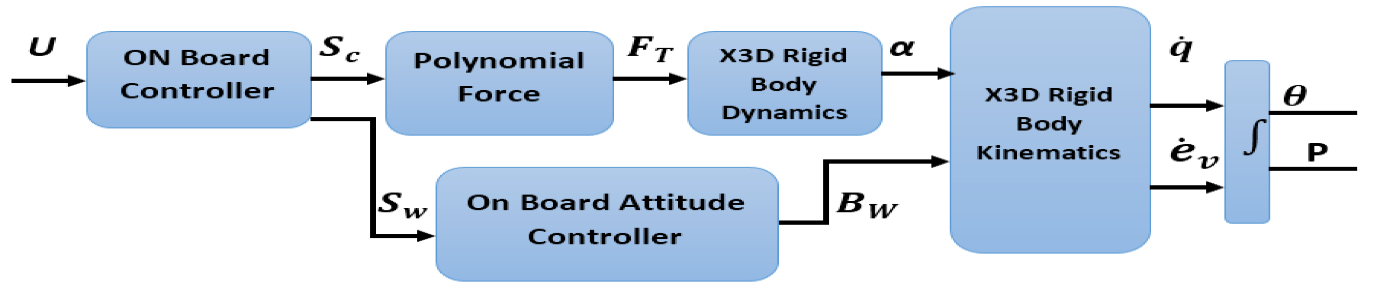
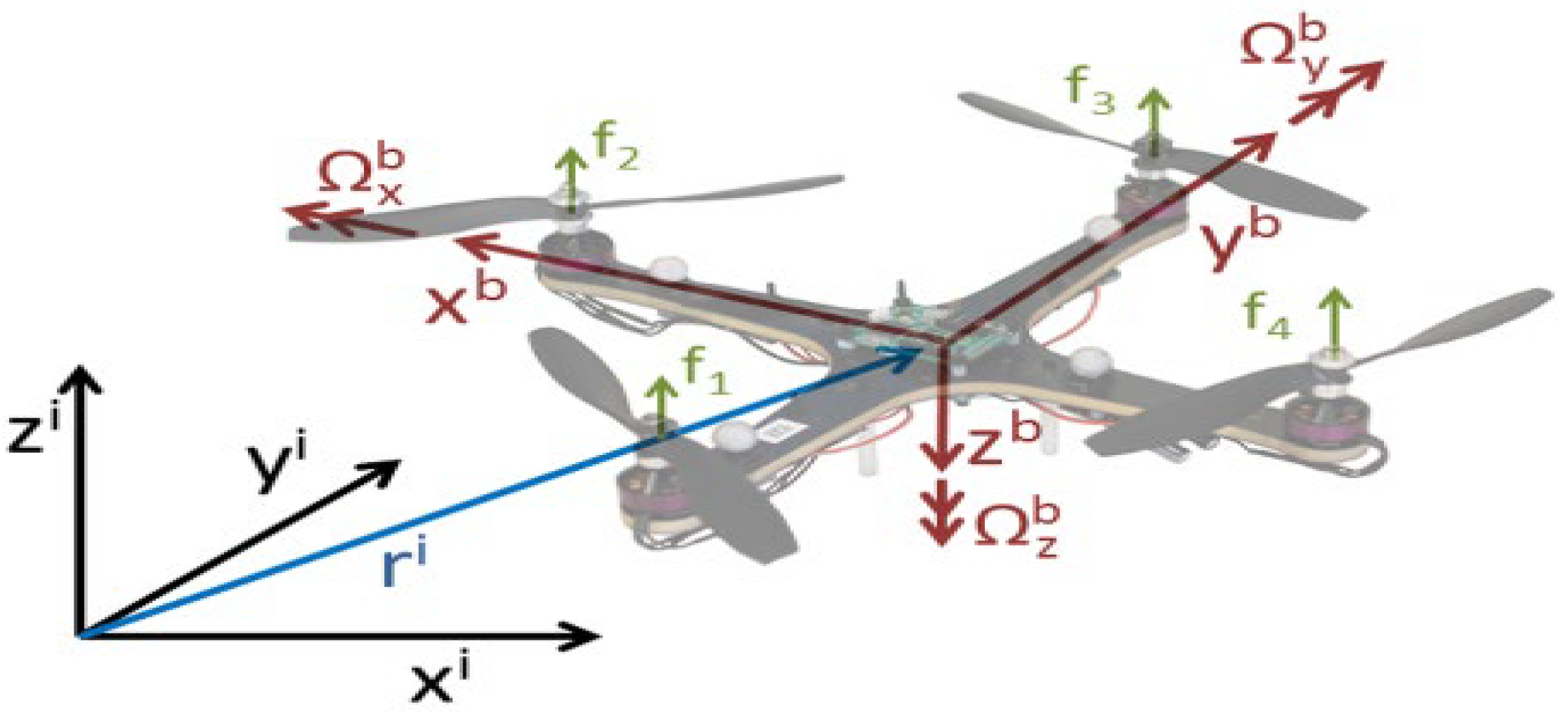
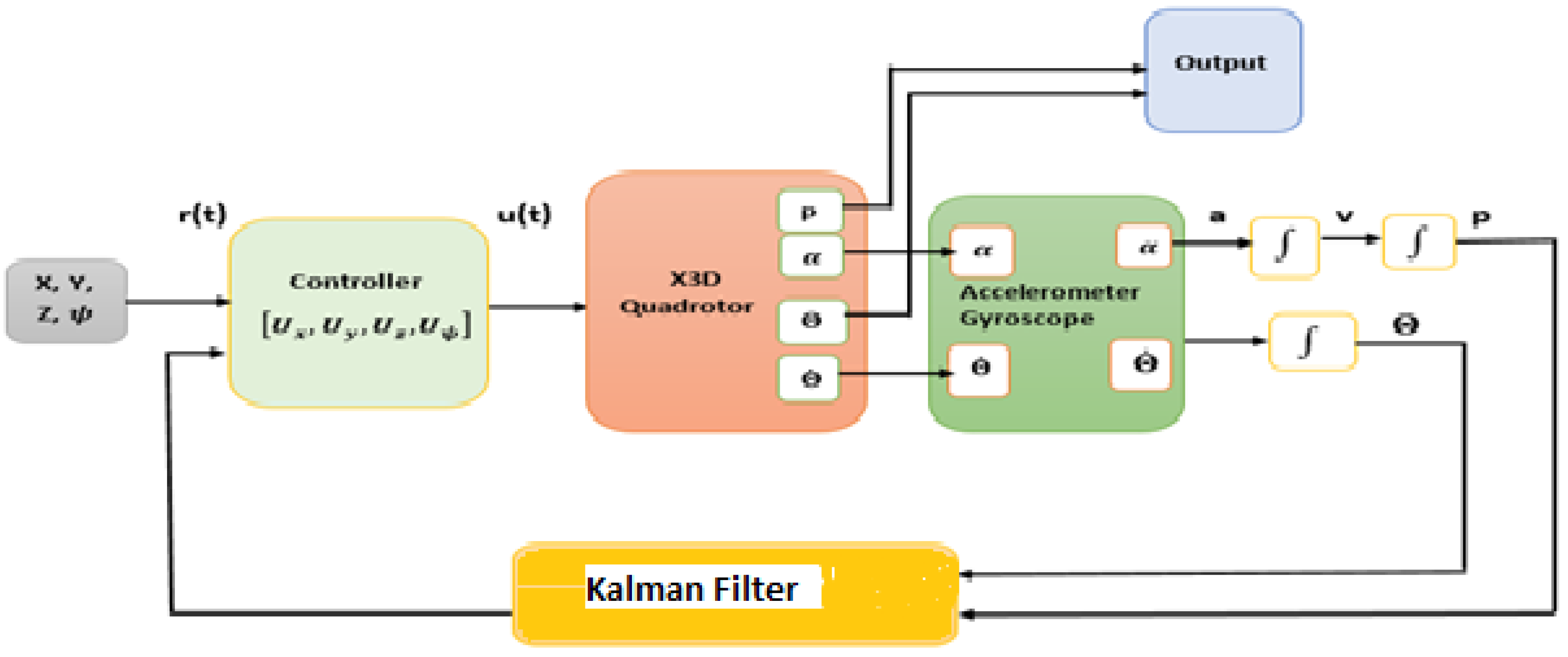
2. Mathematical Modeling of X3d Quadrotor

Kinematics and dynamics are the two parts of the X3D model system and are described using the Newton–Euler theorem rules as: (1) A quadrotor has a symmetrical and rigid frame, (2) the quadrotor’s center of gravity is the same as the body’s fixed frame origin, (3) the propellers have a rigid design, (4) the square of the propeller’s speed determines thrust and drag. The X3D quadrotor parameter list is mentioned in Table 2. The complexity of the re-evaluated X3D model, as illustrated in Figure 1, has been significantly decreased. Equation (1) gives the onboard controller’s input vector.
U = [ U ϕ   , U θ   , U ψ   , U t h r u s t ]
The angular velocity (Sω) and collective thrust ( S c ) outputs of the onboard controller are delivered from the kinematics of the reference body X3D, which results in the system’s final output in terms of translation position (P) and orientation (Θ). The Newton–Euler formulation provides a comprehensive mathematical account of quadrotor dynamics [14]. Position, Euler angle, linear velocity, and angular velocity are among the 12-degree-of-freedom output states described by Equation (2).
12 D O F = [ x , y , z , ϕ , θ , ψ , x ˙ , y ˙ , z ˙ , ϕ ˙ , θ ˙ , ψ ˙ ]
The right-handed system is the inertial (Earth) frame of reference E = [ O e , X e   , Y e , Z e ] and denotes the origin, which is the center of the earth. Its purpose is to determine the quadrotor’s location. Right-handedness is reflected in the bodily frame of reference as B = [ O B , X B   , Y B , Z B ] and denotes the origin, which is located at the quadrotor’s center of gravity. It is used to figure out the quadrotor’s orientation with the earth frame.
In the body frame, the torque, the force F B , angular velocity ω B , and linear velocity v B are all computed. The body and the earth reference frames are shown in Figure 2. The coordinates of the quadrotor (body frame) can be aligned with the earth frame in the following sequence: Z e on the earth, the frame is aligned to the yaw angle on the body frame Z B (positive ψ),   Y e is aligned to the pitch angle on   Y B (positive θ), and X e is aligned to the roll angle on X B (positive φ). Rotation matrices ( x ϕ D , y θ D , z ψ D ) about the three axes (roll, pitch, and yaw) are described in Equation (3).
x ϕ D = [ 1   0   0   0   c o s   c o s   ϕ s i n   s i n   ϕ 0   s i n   s i n   ϕ c o s   c o s   ϕ ] y θ D = [ c o s   c o s   θ 0   s i n   s i n   θ 0   1   0   s i n   s i n   θ 0   c o s   c o s   θ ]   z ψ D = [ c o s   c o s   ψ s i n   s i n   ψ 0   s i n   s i n   ψ c o s   c o s   ψ 0   0   0   1   ]
By multiplying a frame with a direction cosine matrix (DCM), a reference frame may be converted from earth to body and vice versa (DCM) [1] as in Equation (4).
D C M = E B D ( Θ ) = ( x ϕ D ) . ( y θ D ) . ( z ψ D )
Equation (5) gives an orthogonal rotation matrix from the body frame to the inertia (earth) frame.
E B D ( Θ ) = [ c o s   c o s   θ   c o s   c o s   ψ c o s   θ   s i n   s i n   ψ s i n   s i n   θ s i n   s i n   ϕ s i n   s i n   θ   s i n   s i n   ψ   c o s   c o s   ϕ   s i n   s i n   ψ s i n   s i n   ϕ   s i n   s i n   θ   s i n   s i n   ψ   + c o s   c o s   ϕ   c o s   c o s   ψ s i n   s i n   ϕ c o s   c o s   θ   c o s   ϕ   s i n   s i n   θ   c o s   c o s   ψ   + s i n   s i n   ϕ   s i n   s i n   ψ s i n   s i n   ϕ   c o s   c o s   θ c o s   ϕ   c o s   c o s   θ ]
In Equation (6), the translational velocity V E of the X3D is given about the earth frame.
V E = P ˙ = B E D ( Θ ) . V B
Equations (7) and (8) can be used to convert angular velocities in the body frame to angular velocities in the earth frame.
( Θ ˙ ) = B E H ( Θ ) . B ω
[ ϕ ˙   θ ˙   ψ ˙   ] = [ 1   θ   ϕ     θ   ϕ     0   ϕ   ϕ     0   ϕ   θ     ϕ   θ     ] [ p   q   r   ]
Equation (9) can be used to compute the angular velocity in the body frame.
B ω = S ω   .   K ω
Equation (10) can be used to determine the angular velocity in the earth frame.
E ω = Θ ˙ = B E H ( Θ ) . B ω
All external forces are added together to provide the overall force operating on the X3D quadrotor. As seen in Equation (11).
T o t B F = R o t o r B F + g B F
where R o t o r B F = 1 B F + 2 B F + 3 B F + 4 B F .
The upward forces created by the X3D rotors are 1 B F   t o   4 B F , and F g is the force impacting the body. The angular velocity of rotors affects the R o t o r B F .
The nonlinear Simulink model of the x3D quadrotor is presented in Figure 3. The nonlinear dynamic equations of the x3D quadrotor are linearized using a first-order Taylor approximation to implement the linear controller. The X3D near the hover position’s aggregate linearized equations may be expressed as Equation (14):
x ˙ = V x   ,   y ˙ = V y   ,   z ˙ = V z ϕ ˙ = p ,   θ ˙ = q   ,   ψ ˙ = r V ˙ x = ϕ g   V ˙ y = θ g   V ˙ z = F z + I f   .   V Z m  

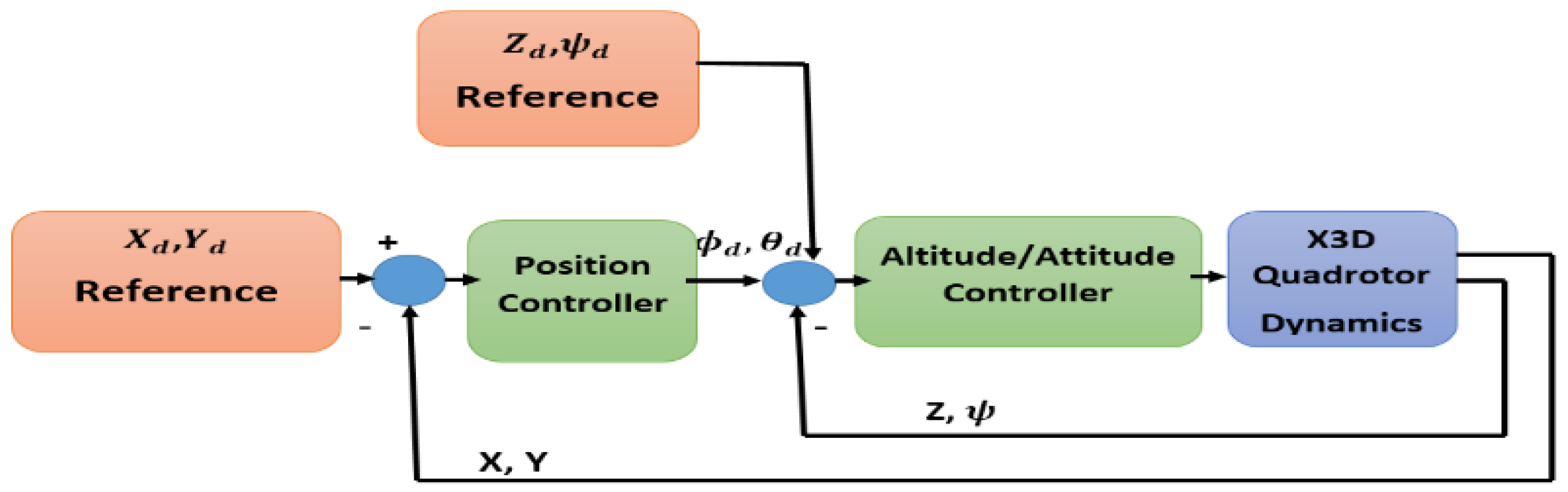
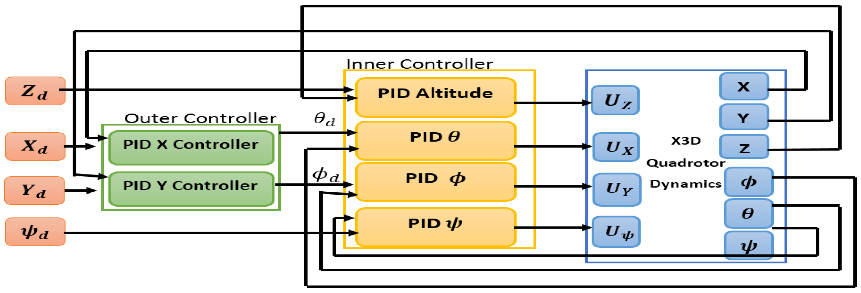
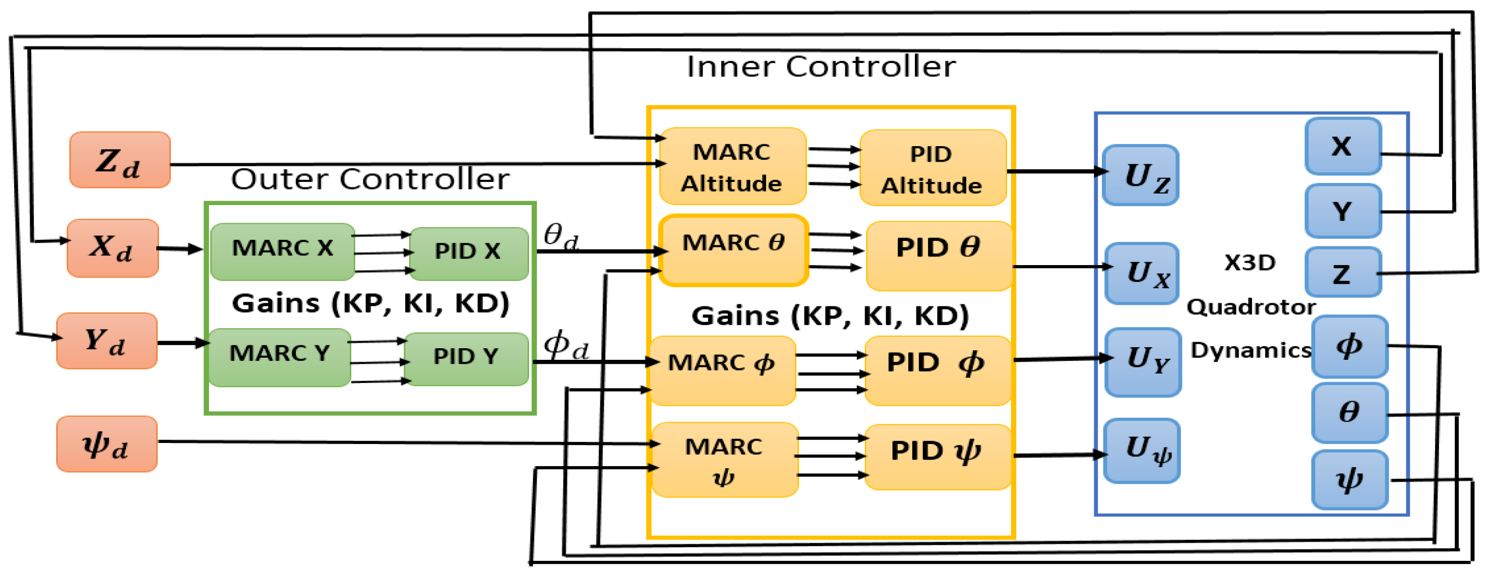
3. X3D Quadrotor Controller Design

For an X3D quadrotor control system, two control loops are suggested, as shown in Figure 4. The position controller in the outer control loop controls the system’s slower dynamics (longitudinal and lateral translations), while the attitude/altitude controller in the inner control loop controls the system’s quicker dynamics (attitude and altitude).
The quadrotor’s intended rotor speed is output by the attitude/altitude controller. The PID controller, LQR controller, fuzzy logic controller, and model reference adaptive PID using MIT rule controller were used in this research to stabilize the translation position and attitude/altitude of an X3D quadrotor.

3.1. PID Control System

PID controllers are the most fundamental feedback controllers that are frequently utilized in many industrial applications [22]. A PID controller calculates an error value that distinguishes between the desired set point and the measured process value. By changing the process control inputs, the controller tries to decrease the error. To use the PID controller for achieving ideal values for a better control system, a complete mathematical model of the plant is required to determine the three parameters (proportional gain K P , integral gain   K I , and derivative gain K D ) [23]. Six PID controllers for attitude/altitude stabilization and translation trajectories are presented in this research. The attitude angles are controlled by three PID controllers ( ϕ , θ   a n d   ψ ) . The altitude (z-axis) of the X3D quadrotor is controlled by one PID controller, while the longitudinal and lateral positions (x-axis and y-axis) are controlled by two PID controllers. Hence, the attitude is determined by the positions. The Euler angles’ preliminary conditions are set to (0, 0, and 0) to begin the experiment. The angular velocity and thrust for the X3D quadrotor are then generated by combining all PID controllers with the combinational control. Figure 5 depicts the PID controller feedback loops for an X3D quadrotor [24]. Equation (13) illustrates the discrete-time transfer function for each PID controller.
P I D = ( K P + Z 1 K D + 1 Z 1 K I )
In Equations (14) and (15), the equations for PID attitude control are provided.
e a t t i t u d e = Θ r e f r e a n c e Θ m e a s u r e d   .   E B D ( Θ )  
  Θ d e s i r e = e a t t i t u d e . P I D
Similar to PID for attitude control, PID for height control ( z- a x i s ) and PID for translation position control ( x- a x i s   a n d   y- a x i s ) are calculated. The height ( z- a x i s ) and intended angular velocity are used as inputs in the combination control step, and following saturation, thrust and the actual angular velocity are transmitted to the X3D quadrotor’s nonlinear model, as shown in Equations (16)–(18). The classical discrete PID is implemented in all the controller blocks, and the parametric gain values are listed in Table 3.
ω d e s i r e = ( Θ d e s i r e Θ m e a s u r e d ) . E B H ( Θ )
U [ X ,   Y , ψ ] = s a t { ω d e s i r e }
  U Z = s a t { Z d e s i r e }

3.2. LQR Control System

The linear quadratic regulator (LQR) controller has been widely used in engineering applications such as voltage source inverters and wheeled inverted pendulum vehicles [25]. There is comparably little research on using the LQR control technique to track and stabilize the quadrotor. The LQR control system is designed to give optimum control while being cost-effective [26]. Owing to the significant uncertainties and nonlinearities in quadrotor dynamics, as well as model unreliability due to parameter fluctuations and linearity approximation, implementing the LQR control system on the quadrotor is a difficult undertaking. As a result, the quadrotor system dynamics are described by a linear state–space equation, with a quadratic cost function as the least appropriate cost function [27]. Equations (19) and (20) depicts the form of the continuous state–space model:
x ˙ s ( t ) = A x s ( t ) + B u ( t )
y ( t ) = C x s ( t ) + D u ( t )
To develop the continuous state–space model, the X3D’s linearized state–space Equation (21) and (22) is employed. The A matrix is shown below, with C = I 9 X 9   a n d   D = 0 9 x 4 as the C and D matrices, respectively.
x ˙ s ( t ) =       A     x s ( t )
[ x ˙   y ˙   z ˙   ϕ ˙   θ ˙   ψ ˙   V x ˙   V y ˙   V z ˙   ] = [ 0   0   0   0   0   0   0   0   0 0   0   0 0   0   0 0   0   0 1   0   0   0   1   0   0   0   1 0   0   0   0   0   0   0   0   0   0   0   0   0   0   0   0   0   0 0   0   0   0   0   0   0   0   0 0   0   0   0   0   g   0   0   0   g   0   0 0   0   0 0   0   0 0   0   0   0   0   0   0   0   I f m ] [ x   y   z   ϕ   θ   ψ   V x   V y   V z ]
Equation (23) derives the discrete case quadratic cost function.
J = k = 0 | x k T Q x k + u k T R u k
The weighted matrices of the state vector and input vector, respectively, are Q and R . The Q and R gain matrices for simulation were determined using Bryson’s method. Equation (24) yields the Q and R gain matrices for the X3D quadrotor.
Q = [ 10   0   0   0   10   0   0   20 0   0   0   0   0   0   0   0   0 0   0   0   0   0   0   0   0   0 0   0   0   0   0   0   0   0   0 5   0   0   0   5   0   0   0   10 0   0   0   0   0   0   0   0   0 0   0   0   0   0   0   0   0   0 0   0   0   0   0   0   0   0   0 1   0   0   0   1   0   0   0   1 = [ 10   0   0   10 0   0   0   0 0   0   0   0 10   0   0   10 ]
The parameters k , P , and e for the LQR system may be retrieved using the MATLAB l q r function, as indicated in Equation (25).
[ k , P , e ] = l q r ( A , B , Q , R )

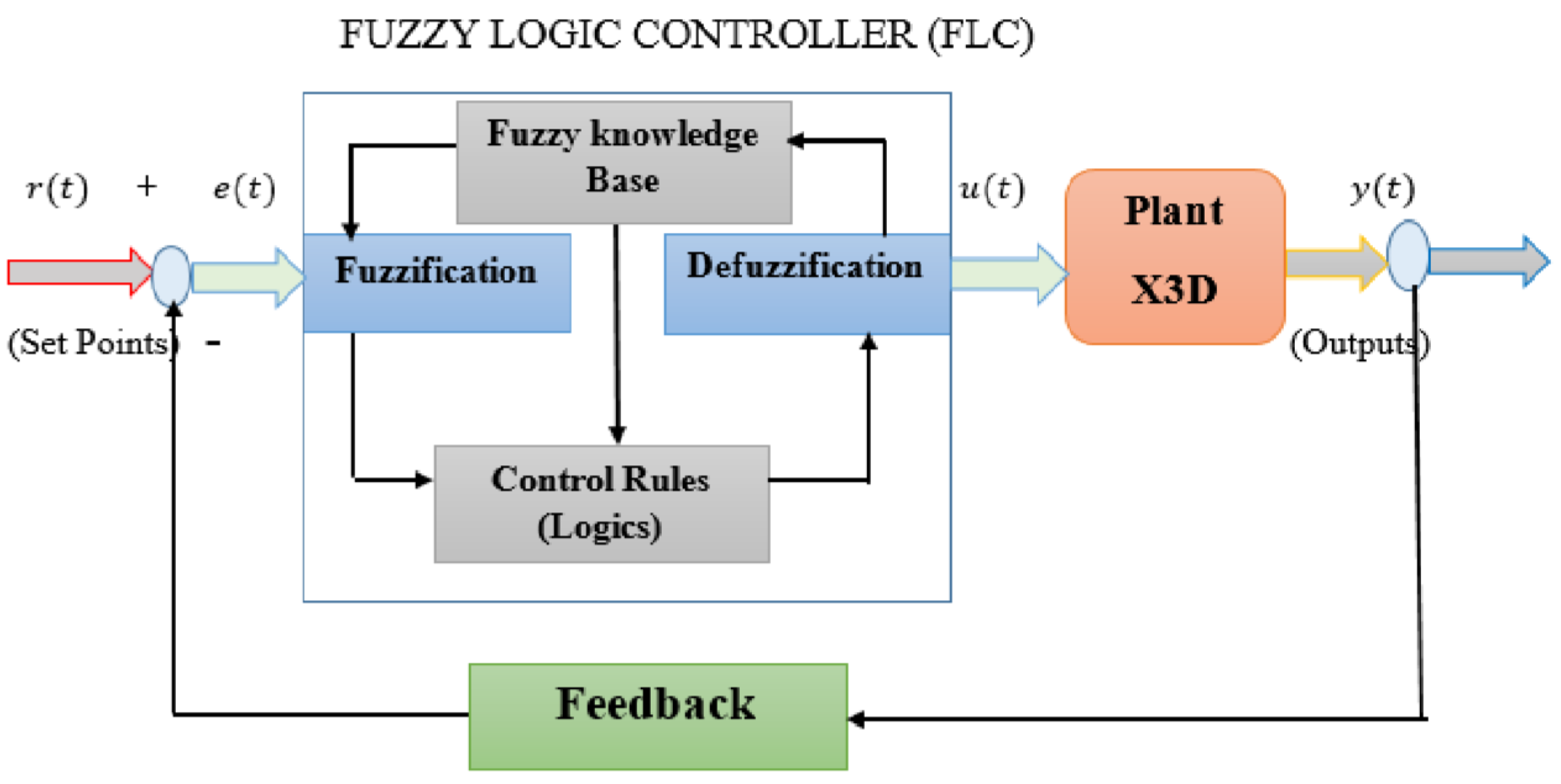
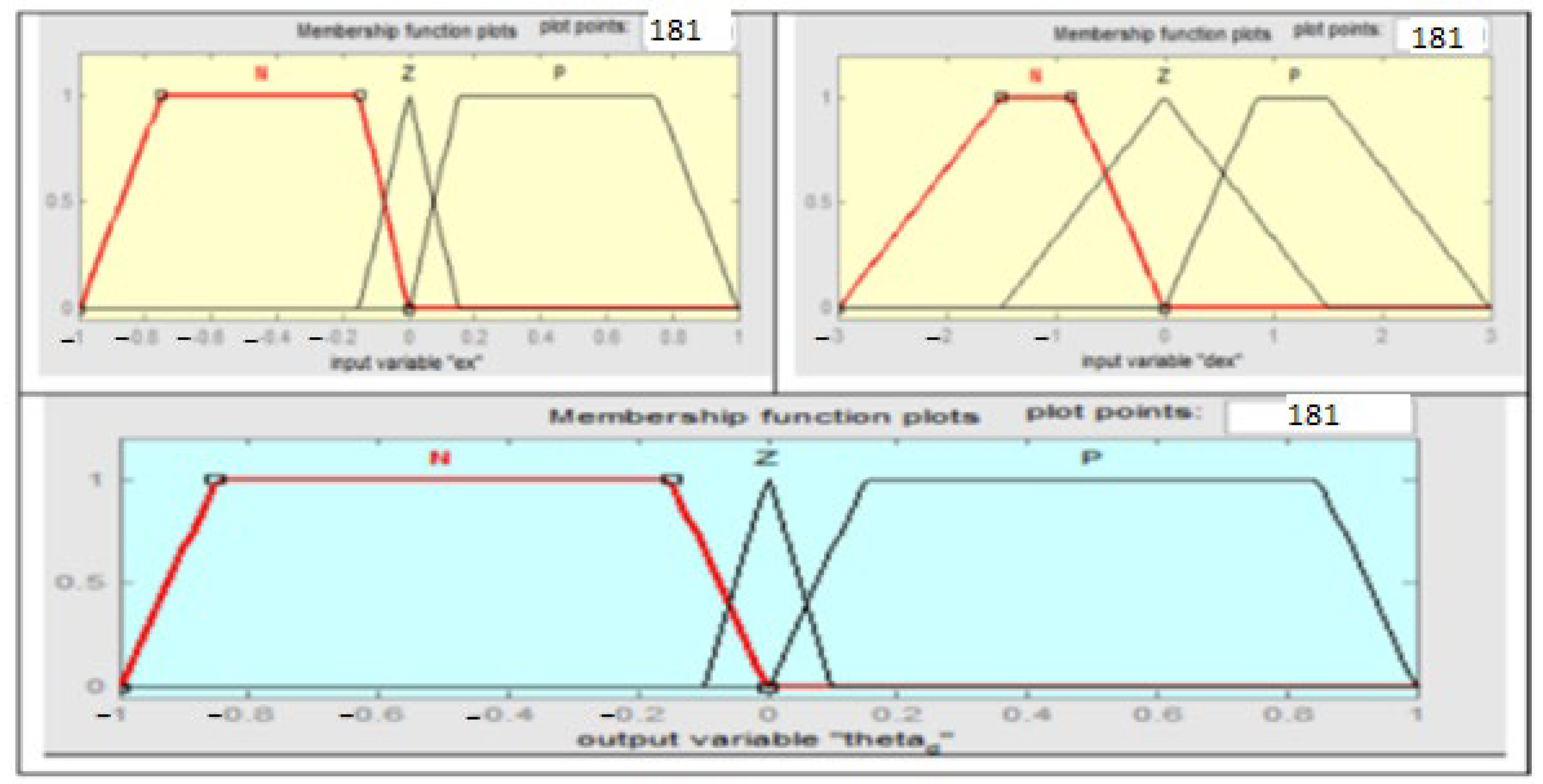
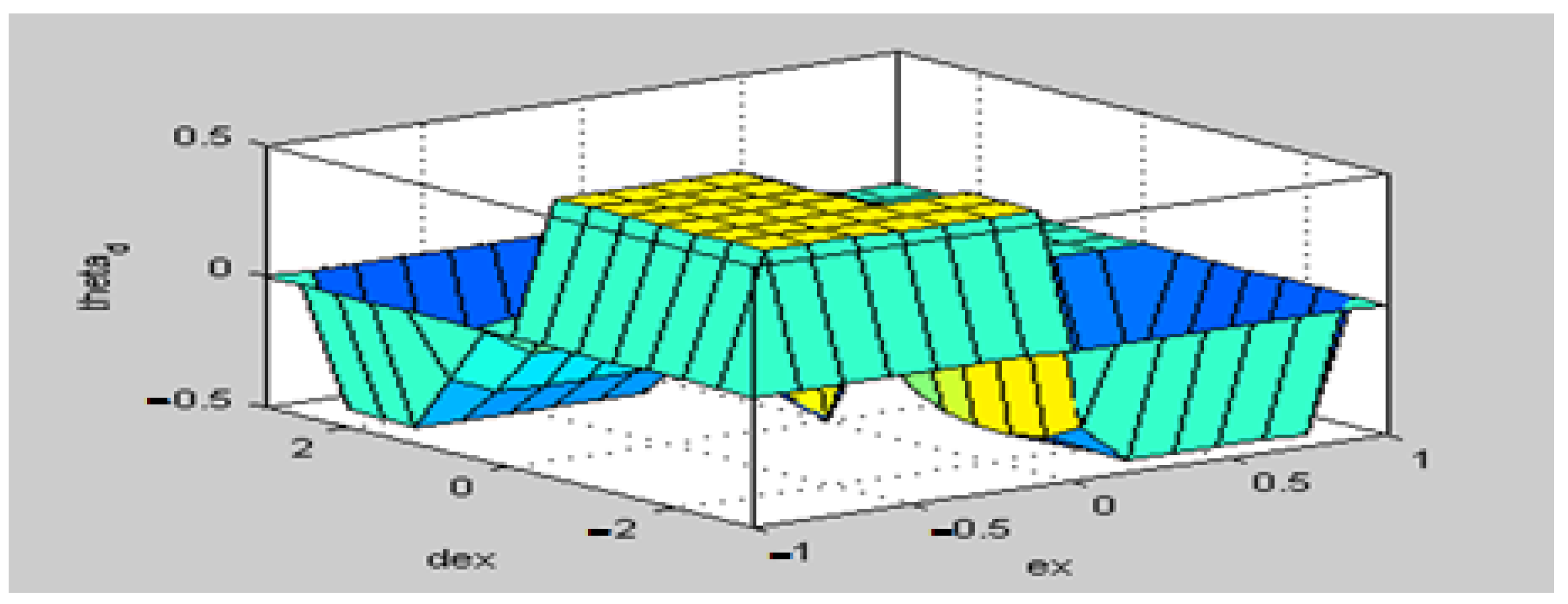
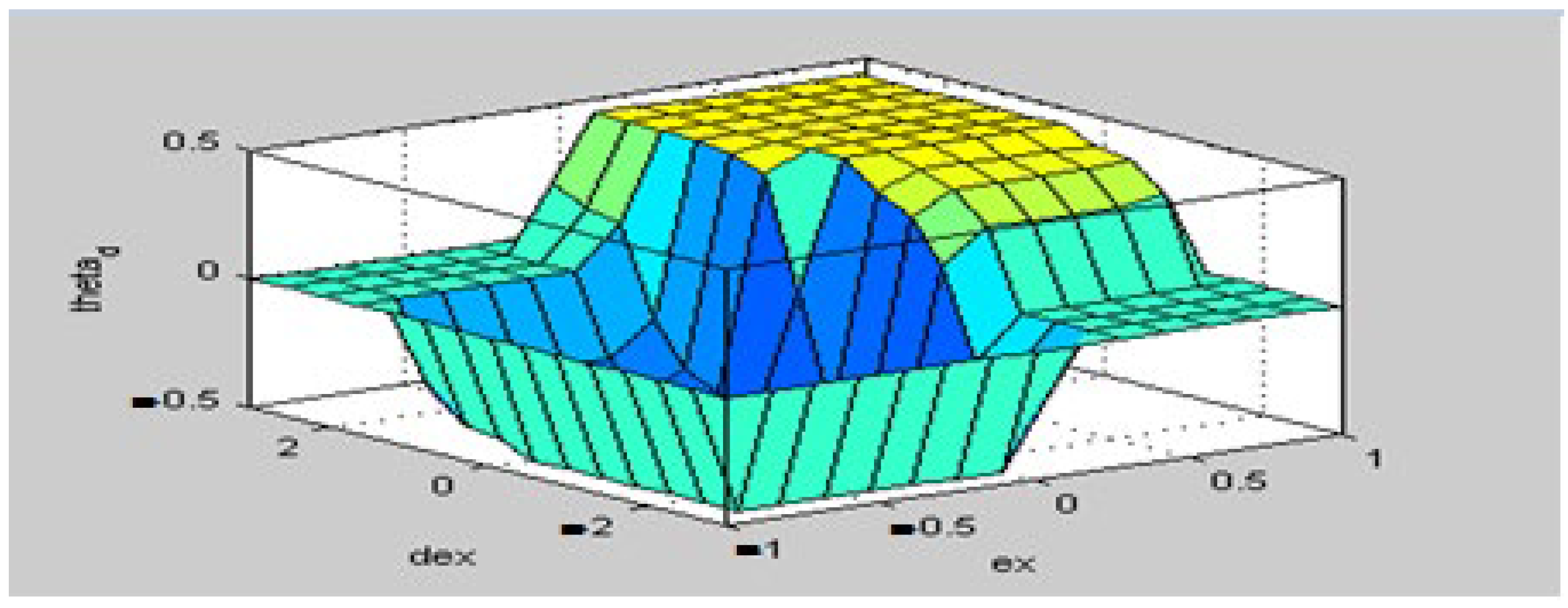
3.3. Fuzzy Logic Control System

The correlation between the input data and the output action is described using human language descriptions in fuzzy logic. It is a mathematical system that takes analog input values and compares them to variables that need values between 0 and 1 [28]. The proper process input is determined by a fuzzy controller’s fuzzy membership function and inference rule. The quadrotor’s translation position must be controlled while its attitude (roll, pitch, and yaw angle) must be stabilized [29]. In this article, an X3D quadrotor is controlled using Mamdani’s fuzzy inference approach. The quadrotor’s attitude (desired angles of roll, pitch, and yaw) is controlled by three fuzzy controllers, denoted as FC ( ϕ ), FC ( θ ) and FC ( ψ ), respectively (desired angles of roll ϕ , pitch θ , and yaw ψ ) [30]. FC (Z) determines the altitude of the quadrotor. The quadrotor’s translation position is controlled by two additional fuzzy controllers, FC (X) and FC (Y). The states φ and θ are used to control the X and Y positions, respectively. All six fuzzy logical controllers use the same two identical inputs as described below.
  • Error ( e ) denotes the difference between the desired and measured signals.
  • Derivative error ( d e ) is the error rate.
Figure 6 depicts the implementation of a fuzzy system for quadrotor control. Error is stabilized between [−1, +1] and [−3, +3], whereas the error rate is stabilized between [−3, +3].
The output with three fuzzy logic values (N, Z, and P) is used for the input variables e and de, as indicated in Table 4; N stands for negative, Z for zero, and P for positive. Table 1 explains the rules: If the error ( e ) is negative and the rate of error ( d e ) is negative, then the output will be negative. Figure 7 depicts all of the FCs’ controller inputs as well as membership functions.
The surface view of all Fuzzy controllers is shown in Figure 8 and Figure 9.

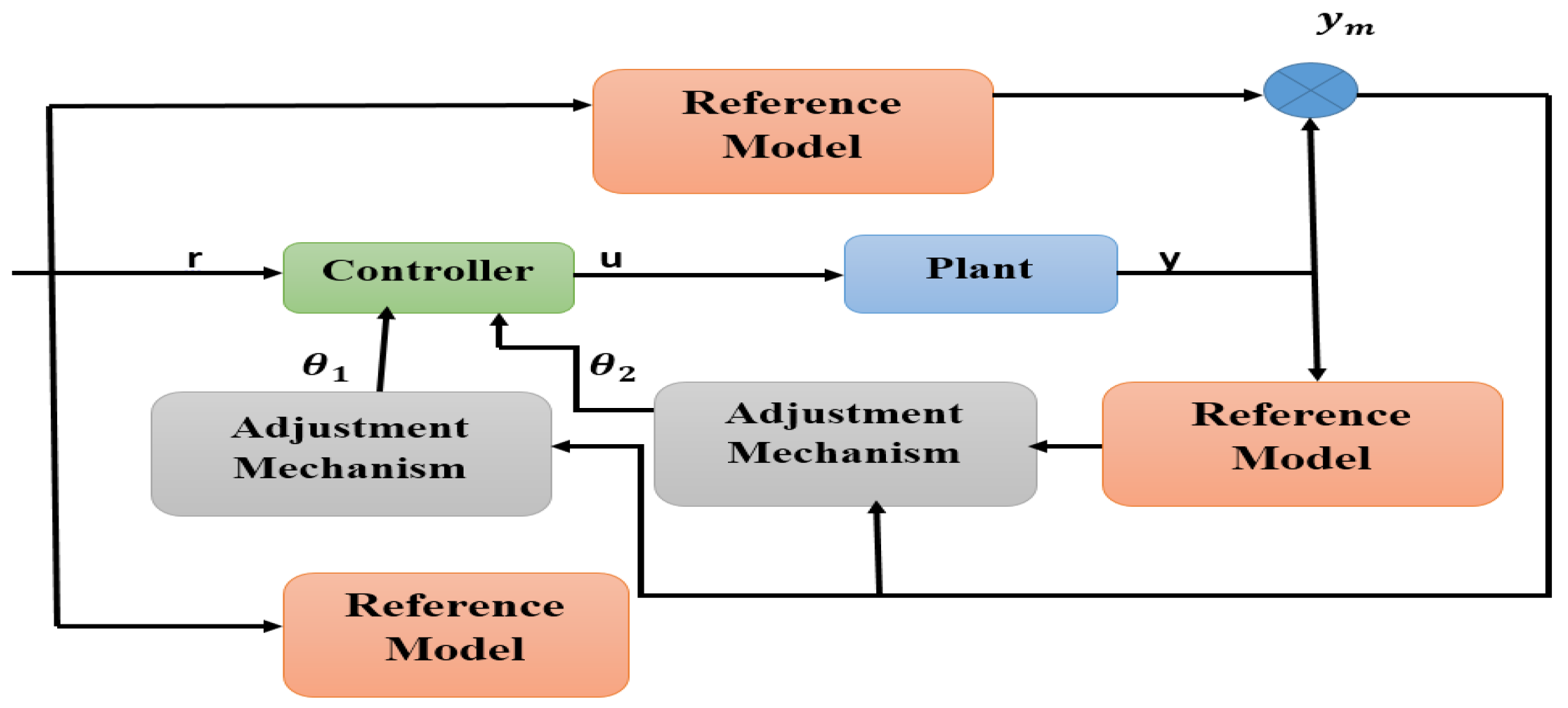
3.4. Model Reference Adaptive PID Control System Based on MIT Rule

Numerous controllers, including PI, PD, PID, and feedback, can be adapted utilizing particular adaptation methods to improve system performance. In this research, the model reference adaptive PID controller based on MIT rule was used to investigate the fast-tracking and stability control of quadrotor [31]. The Massachusetts Institute of Technology (MIT) developed the MRAC-based MIT rule in 1960 [32]. It employs the model reference adaptation control technique to ensure that the actual plant output follows the output of the reference model when the reference inputs are the same for any practical system with undetermined and unpredictable characteristics that can be adjusted by control settings [33] as illustrated in Figure 10. This section presents the MIT-rule-based design parameter adaption rules for a PID controller. The following are the steps to creating an MRAC using the MIT rule. Obtain the MRAC system reference model that yields the desired trajectory y m .
G m ( s ) = y m ( s ) u c ( s ) = α s + ω n 2 s 2 + 2 s ζ ω n + ω n 2  
Closed-loop characteristics such as settling time t S and overshoot (OS) are used to estimate the damping ratio ζ and natural frequency ω n . Table 5 lists the specifications of the reference model for the X3D quadrotor.
The transfer function of the reference model is changed as follows:
  G m ( s ) = y m ( s ) u c ( s ) = 0.1058 s 2 + 0.1496 + 0.1058  
  • State the adaptive law of MRAC system for PID controller as
    u ( t ) = K P e ( t ) + K I 0 t e ( t ) d t K D d y p d t  
    where   e ( t ) = u c y p
The PID controller’s transfer function in Laplace domain is described in Equation (29)
U ( s ) = K P E + K I s E K D s y p  
2.
State the tracking error e for the system as
e = r y p
where r is the system reference input.
d e d t = d y p d t  
3.
As stated in Equation (34), estimate the adaption error ε .
ε = y p y m
where y p denotes the plant output and y m denotes the reference model output.
4.
As follows, describe the MIT rule, which is described as the temporal rate Φ of change proportional to the cost function’s ( J ) negative gradient.
      d Φ d t = γ J Φ = γ e e   Φ
For calculating the value of PID controller parameters ( K ˙ P ,   K ˙ D ,   K ˙ I ), use the MIT Rule (gradient method). The following are the estimated adjustment parameters.
d K p d t = γ p ε ( s s 2 + 2 s ζ ω n + ω n 2 ) e d K I d t = ( γ I ) ε ( 1 s 2 + 2 s ζ ω n + ω n 2 ) e d K D d t = γ D ε ( s 2 s 2 + 2 s ζ ω n + ω n 2 ) y p  
For the approximate parameters K P , K I   a n d   K D of adaptation, the law is as (35).
θ 1 = K p = ( γ p s ) ε ( s s 2 + 2 s ζ ω n + ω n 2 ) e θ 2 = K I = ( γ I s ) ε ( 1 s 2 + 2 s ζ ω n + ω n 2 ) e θ 3 = K D = ( γ p s ) ε ( s 2 s 2 + 2 s ζ ω n + ω n 2 ) y p  
The value of the adaptation gain ( γ ) has a direct relationship with the convergence rate.
The simulation results show that it is correct for small values ( γ ) but impulsive for high values, indicating that the right selection of ( γ ) is critical. The quadrotor’s attitude (roll ϕ , pitch θ , and yaw ψ ) is controlled by three MARC adaptive PID controllers, indicated by M A R C   ϕ ,   M A R C   θ   a n d   M A R C   ψ , respectively. MARC Z oversees controlling the quadrotor’s height, while MARC X and MARC Y are in charge of controlling the quadrotor’s position. The architecture of the MARC adaptive PID controller with MIT rule including all six degrees of freedom (DOF) quadrotor output is shown in Figure 11. Three PID controller parameters ( K P   , K I ,   a n d   K d ) can be modified using the MARC system and the MIT rule to make the nonlinear X3D Quadrotor stable and track to the appropriate reference input.

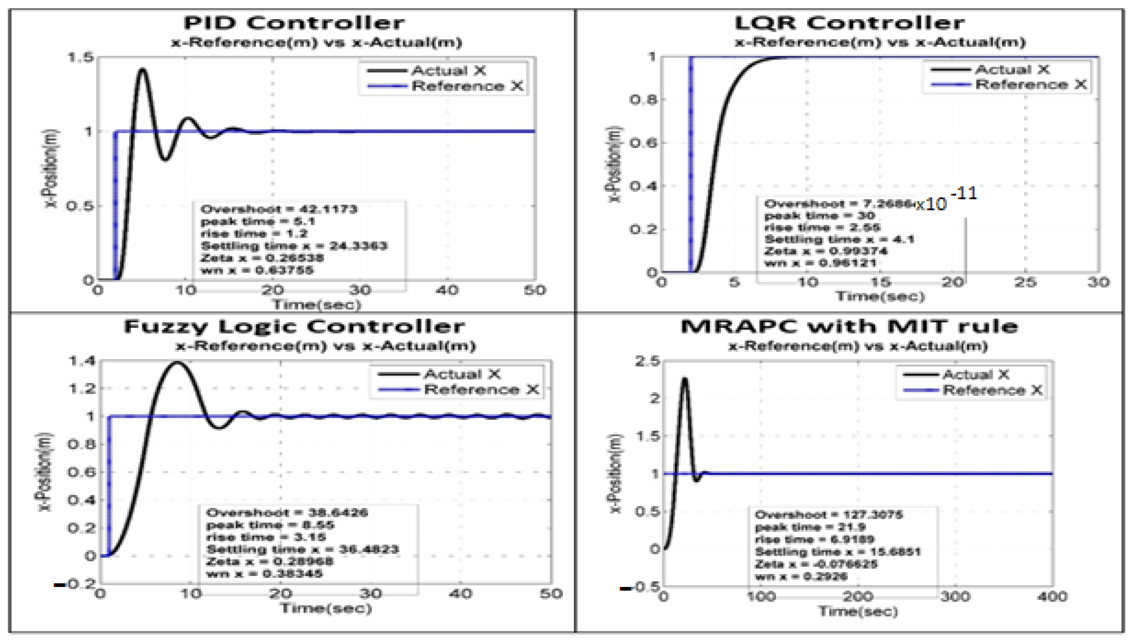
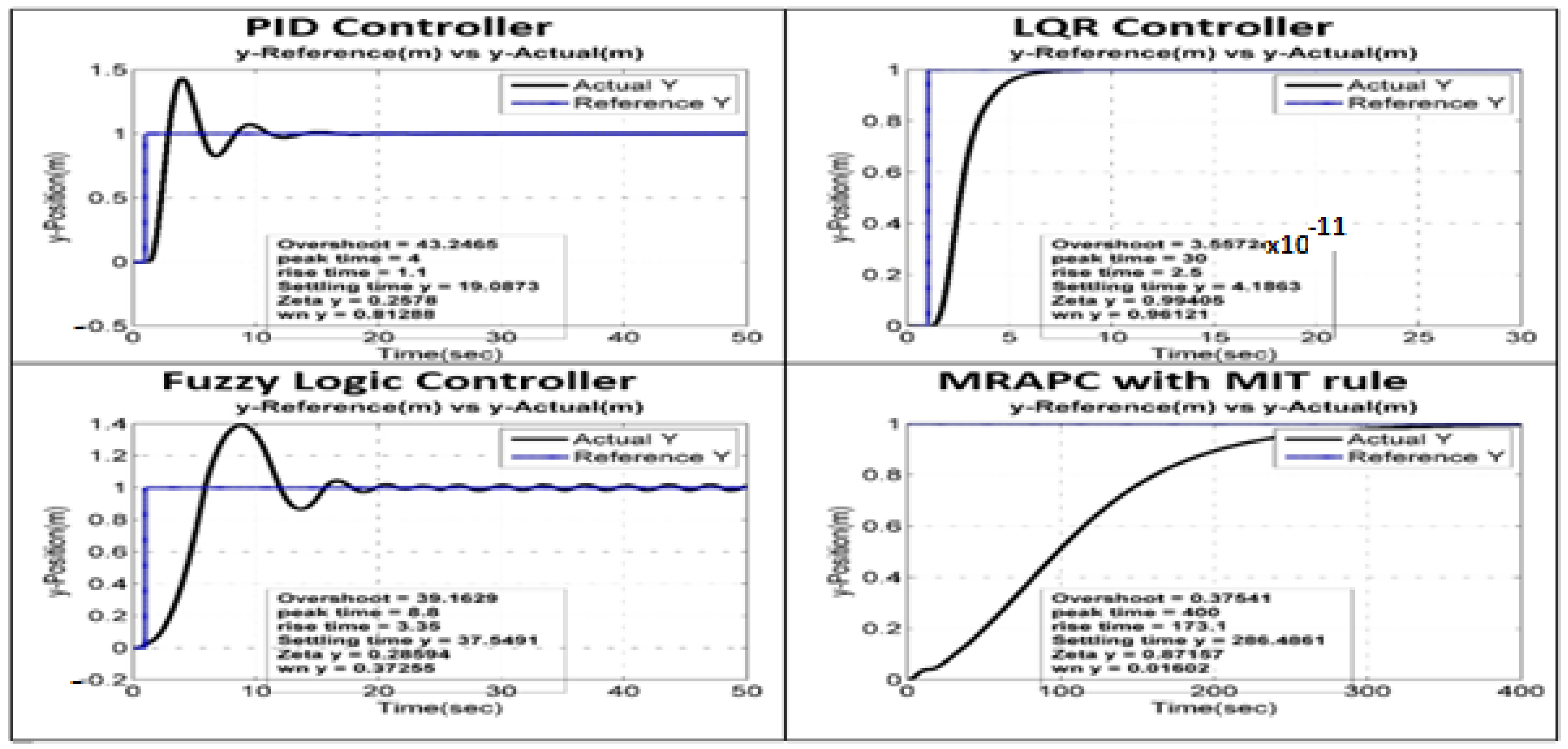
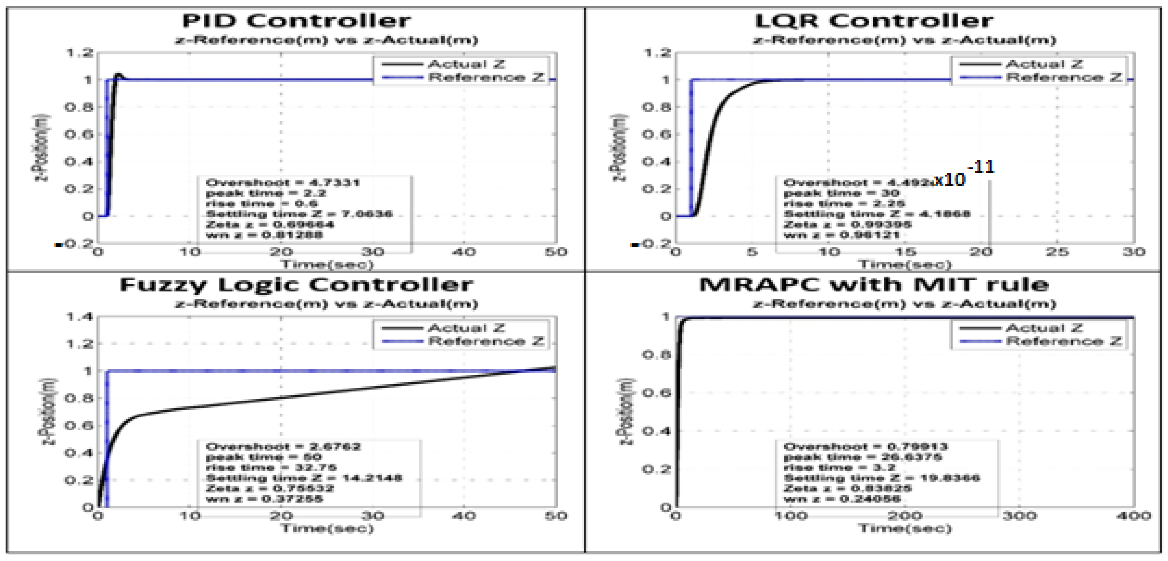
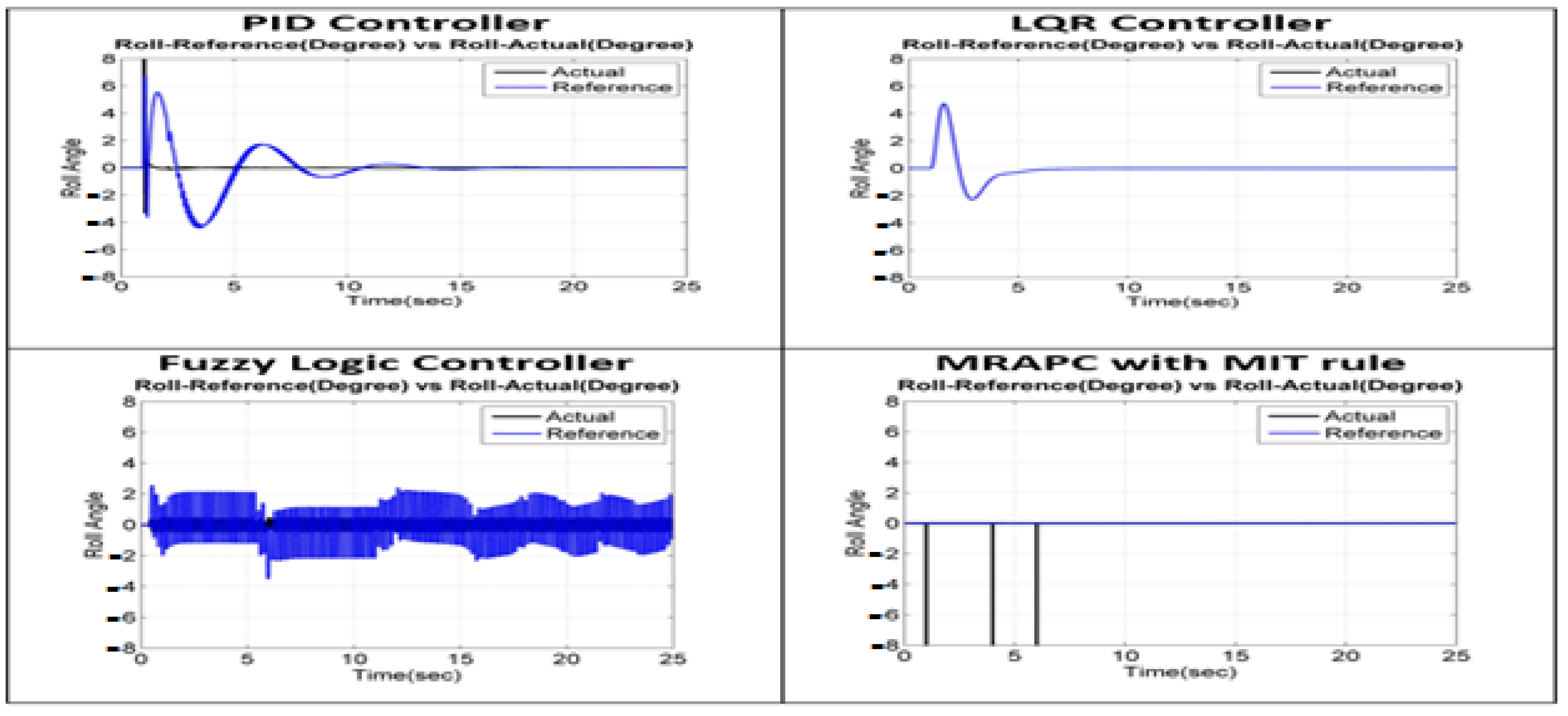
4. Simulation Results

All linear and nonlinear controllers can provide system stability and optimum performance under their nominal conditions. It is indeed challenging to obtain equivalent results from both the simulation and the real-time experiment due to highly precise parameter adjustment and nonlinear parameters and dynamics. Researchers generally use modelled linear controllers because of their simplicity of design and implementation, as well as their ability to produce high-quality experimental data. On the other hand, robustness, noise and disturbance elimination, limitation control at the endpoints, and more precise trajectory tracking are all advantages of nonlinear controllers [34,35,36]. Therefore, theoretical studies reveal that linear controllers such as LQR and PID are good at maintaining stability under nominal conditions but not so good at ensuring robustness. The fuzzy controller, on the other hand, cannot guarantee nominal stability but can offer adequate and excellent maneuvering performance. Furthermore, hybrid and adaptive controllers are created as units in which many controllers can work together to provide the finest balance of robustness, nominal stability, flexibility, optimality, simplicity, tracking ability, rapid response, and disturbance rejection to a system, among other features. High computation, a large amount of training data, estimation error, and the existence of uncertainty are the issues that these controllers must confront to achieve satisfying performance, even though they are capable of ensuring remarkable outcomes when the system is disturbed by uncertainty. For example, LQR becomes LQG when the Kalman filter is used to generate a state observer and eliminate signal noise. Secondly, to achieve excellent maneuvering performance, a model reference adaptive controller is used to update the PID controller gain. Figure 12 shows the proposed control structure, which includes a control unit, an X3D Quadrotor, an inertial measurement unit (IMU), and a Kalman filter. The reference input will be received first by the quadrotor system. It measures the translational position and rotational position, velocities, and accelerations of the X3D Quadrotor at a specified time. The output of the quadrotor is then sent to the IMU sensor, which includes a three-axis accelerometer and a gyroscope. The Kalman filter is used to rectify and filter the output of an IMU sensor before it is fed back to the control unit. The control unit then generates an output that is equivalent to the thrust that all motors must provide in order to maintain the well-defined requirements of the X3D quadrotor. The proposed control structure mentioned above is implemented in the MATLAB Simulink environment. To evaluate the performance of all control systems for the specified reference position, unit step tests are performed in all the three axes, x, y, and z. Desired references for step input at the xyz positions are set to 1. The simulation period of an X3D Quadrotor system is defined as 30, 50, and 400 s, correspondingly, for positional testing (x, y, and z) among suggested controllers.
Figure 13, Figure 14, Figure 15, Figure 16, Figure 17 and Figure 18 illustrate the output response of the closed-loop control system for the longitudinal position (x-axis), lateral position (y-axis), altitude (z-axis), and attitude (roll, pitch, and yaw angle) for each of the four controllers. All controllers work well in keeping the quadrotor in the proper reference position, as can be seen in these figures. Table 6, Table 7 and Table 8 provides the comparison of step test results in terms of rising time, settling time, peak time, and overshoot for all three dimensions (x, y, and z). Figure 13 and Figure 14 show the X and Y position responses, whereas Figure 15 shows the height (z-axis) response.
The aggregate performance of the PID controller, LQR controller, fuzzy controller, and MRAPC with MIT rule controller appears to be satisfactory, as demonstrated in Figure 13 and Table 6, where the root mean square error (RMSE) and normalized root mean square error (NRMSE) for simulations are less than 1 m along the x-axis. Although, the LQR controller is superior to others because it reduces overshoot, rising time, and settling time along the x-axis. Nevertheless, the performance of PID, LQR, fuzzy, and MRAPC with MIT rule appears to be good, as demonstrated in Figure 14 and Table 7, where the root mean square error (RMSE) and normalized root mean square error (RMSE) for simulations are below 1 m along the y-axis.
In terms of overshoot, rising time, and settling time along the y-axis, the LQR controller performs better.
According to Figure 15 and Table 8, the LQR controller achieves superior results along the z-axis than other control approaches because there is no overshoot, the rising time is shorter, and the settling time is shorter. In Figure 16, the LQR controller stabilizes the roll angle in 4 s, which is a much quicker period than the findings of other controllers.
The LQR controller, as shown in Figure 17, requires a shorter time to stabilize the pitch angle than other controllers.
Figure 18 demonstrates that the system has a negligible yaw angle in the case of the LQR controller structure.

5. Conclusions

The system proposed in this manuscript is a quadrotor. Controlling and stabilizing the quadrotor is a substantial issue due to nonlinearity and under-actuated configurations, such as a lower number of control inputs than degrees of freedom (DOF). A comparison of four alternative control methods, such as the LQR controller, PID controller, fuzzy controller, and model reference adaptive PID controller using the MIT rule, has been provided in this article for an X3D quadrotor. These controllers demonstrate the stability, robustness, and control of a quadrotor during maneuvers and trajectory tracking in the presence of nonlinear dynamics. The results of simulations demonstrate that given the identical translation position, altitude, and attitude inputs, each control system responds differently. However, based on the features that are required for the quadrotor application, it is possible to select the most suited system. When compared to other controllers at almost the same operating conditions, the LQR controller yields the highest accuracy in x, y, and z-step performance. The LQR controller has a 0.0% overshoot and a 4.1% shorter settling time than other controllers, particularly nonlinear controllers. In terms of the highest settling time and overshoot, the model reference adaptive PID controller using the MIT rule performs the worst. It is worth mentioning that the linear controller methods are quite ubiquitous and easy to implement, and they may be used for a wide range of real-world control systems. For potential research directions, all the controllers will be deployed on the X3D quadrotor board, and the X3D quadrotor’s real-time performance, validation, and authentication of all control systems will be monitored; in addition, other machine learning and deep learning algorithms will be implemented for autonomous operation.

Author Contributions

Conceptualization, T.S., J.A., M.H.J., A.U.R., E.T.E., N.A.G., and M.S.; methodology, T.S., J.A., M.H.J., A.U.R., E.T.E., N.A.G., and M.S.; software, T.S. and J.A.; validation, M.H.J. and A.U.R.; formal analysis, T.S., E.T.E., N.A.G., and M.S.; investigation, M.H.J. and M.S.; resources, E.T.E. and N.A.G.; data curation, T.S. and J.A.; writing—original draft preparation, T.S., J.A., M.H.J., A.U.R., E.T.E., N.A.G., M.S.; T.S., J.A., M.H.J., A.U.R., E.T.E., N.A.G., and M.S.; visualization, M.H.J.; supervision, M.H.J. and M.S.; project administration, E.T.E. and N.A.G.; funding acquisition, E.T.E. and N.A.G. All authors have read and agreed to the published version of the manuscript.

Funding

This research was supported by Future University Researchers Supporting Project Number FUESP-2020/48 at Future University in Egypt, New Cairo 11845, Egypt.

Institutional Review Board Statement

Not applicable.

Informed Consent Statement

Not applicable.

Data Availability Statement

Not applicable.

Conflicts of Interest

The authors declare that they have no conflicts of interest to report regarding the present study.

References

  1. Shakeel, T. Simulated Closed Loop Trajectory Control System of X3D Quadrotor in Ubiquitous Gesture Controlled Environment; COMSATS Institute of Information Technology: Lahore, Pakistan, 2016. [Google Scholar]
  2. Shehzad, M.F.; Bilal, A.; Ahmad, H. Position & attitude control of an aerial robot (quadrotor) with intelligent pid and state feedback lqr controller: A comparative approach. In Proceedings of the 16th International Bhurban Conference on Applied Sciences and Technology (IBCAST), Islamabad, Pakistan, 8–12 January 2019; pp. 340–346. [Google Scholar]
  3. Sain, D.; Mohan, B. Modeling, simulation and experimental realization of a new nonlinear fuzzy PID controller using Center of Gravity defuzzification. ISA Trans. 2021, 110, 319–327. [Google Scholar] [CrossRef] [PubMed]
  4. Zulu, A.; John, S. A review of control algorithms for autonomous quadrotors. Open J. Appl. Sci. 2014, 4, 547–556. [Google Scholar] [CrossRef]
  5. Al-Younes, Y.M.; Al-Jarrah, M.A.; Jhemi, A.A. Linear vs. nonlinear control techniques for a quadrotor vehicle. In Proceedings of the 7th International Symposium on Mechatronics and Its Applications, Sharjah, United Arab Emirates, 20–22 April 2010; pp. 1–10. [Google Scholar]
  6. Argentim, L.M.; Rezende, W.C.; Santos, P.E.; Aguiar, R.A. PID, LQR and LQR-PID on a quadcopter platform. In Proceedings of the 2013 International Conference on Informatics, Electronics and Vision (ICIEV), Dhaka, Bangladesh, 17–18 May 2013; pp. 1–6. [Google Scholar]
  7. Wang, H.; Gelbal, S.Y.; Guvenc, L. Multi-Objective Digital PID Controller Design in Parameter Space and Its Application to Automated Path Following. IEEE Access 2021, 9, 46874–46885. [Google Scholar] [CrossRef]
  8. Jiang, J.; Qi, J.; Song, D.; Han, J. Control platform design and experiment of a quadrotor. In Proceedings of the 32nd Chinese Control Conference, Xi’an, China, 26–28 July 2013; pp. 2974–2979. [Google Scholar]
  9. Khan, A.; Jaffery, M.H.; Javed, Y.; Arshad, J.; Rehman, A.U.; Khan, R.; Bajaj, M.; Kaabar, M.K. Hardware-in-the-Loop Implementation and Performance Evaluation of Three-Phase Hybrid Shunt Active Power Filter for Power Quality Improvement. Math. Probl. Eng. 2021, 2021, 8032793. [Google Scholar] [CrossRef]
  10. Raffo, G.V.; Ortega, M.G.; Rubio, F.R. An integral predictive/nonlinear H∞ control structure for a quadrotor helicopter. Automatica 2010, 46, 29–39. [Google Scholar] [CrossRef]
  11. Sarwar, S.; Javed, M.Y.; Jaffery, M.H.; Arshad, J.; Ur Rehman, A.; Shafiq, M.; Choi, J.-G. A novel hybrid MPPT technique to maximize power harvesting from pv system under partial and complex partial shading. Appl. Sci. 2022, 12, 587. [Google Scholar] [CrossRef]
  12. Menhaj, M.B.; Fakurian, R.S.F. Fuzzy controller design for quadrotor UAVs using minimal control input. Indian J. Sci. Res. 2014, 1, 157–164. [Google Scholar]
  13. Camboim, M.M.; Villanueva, J.M.M.; de Souza, C.P. Fuzzy Controller Applied to a Remote Energy Harvesting Emulation Platform. Sensors 2020, 20, 5874. [Google Scholar] [CrossRef]
  14. Ang, K.H.; Chong, G.; Li, Y. PID control system analysis, design, and technology. IEEE Trans. Control. Syst. Technol. 2005, 13, 559–576. [Google Scholar]
  15. Liu, C.; Pan, J.; Chang, Y. PID and LQR trajectory tracking control for an unmanned quadrotor helicopter: Experimental studies. In Proceedings of the 2016 35th Chinese Control Conference (CCC), Chengdu, China, 27–29 July 2016; pp. 10845–10850. [Google Scholar]
  16. Shi, L.; Zheng, W.X.; Shao, J.; Cheng, Y. Sub-super-stochastic matrix with applications to bipartite tracking control over signed networks. SIAM J. Control. Optim. 2021, 59, 4563–4589. [Google Scholar] [CrossRef]
  17. Shi, L.; Cheng, Y.; Shao, J.; Sheng, H.; Liu, Q. Cucker-Smale flocking over cooperation-competition networks. Automatica 2022, 135, 109988. [Google Scholar] [CrossRef]
  18. Zouaoui, S.; Mohamed, E.; Kouider, B. Easy tracking of UAV using PID controller. Period. Polytech. Transp. Eng. 2019, 47, 171–177. [Google Scholar] [CrossRef]
  19. Kuantama, E.; Tarca, I.; Tarca, R. Feedback linearization LQR control for quadcopter position tracking. In Proceedings of the 2018 5th International Conference on Control, Decision and Information Technologies (CoDIT), Thessaloniki, Greece, 10–13 April 2018; pp. 204–209. [Google Scholar]
  20. Chovancová, A.; Fico, T.; Duchoň, F.; Dekan, M.; Chovanec, Ľ.; Dekanova, M. Control methods comparison for the real quadrotor on an innovative test stand. Appl. Sci. 2020, 10, 2064. [Google Scholar] [CrossRef]
  21. Mahmoud, O.E.; Roman, M.R.; Nasry, J.F. Linear and nonlinear stabilizing control of quadrotor UAV. In Proceedings of the 2014 International Conference on Engineering and Technology (ICET), Cairo, Egypt, 19–20 April 2014; pp. 1–8. [Google Scholar]
  22. Canbek, K.O.; Oniz, Y. Trajectory Tracking of a Quadcopter Using Fuzzy-PD Controller. In Proceedings of the 2021 13th International Conference on Electrical and Electronics Engineering (ELECO), Bursa, Turkey, 25–27 November 2021; pp. 109–113. [Google Scholar]
  23. Salih, A.L.; Moghavvemi, M.; Mohamed, H.A.; Gaeid, K.S. Flight PID controller design for a UAV quadrotor. Sci. Res. Essays 2010, 5, 3660–3667. [Google Scholar]
  24. Aboelhassan, A.; Abdelgeliel, M.; Zakzouk, E.E.; Galea, M. Design and Implementation of Model Predictive Control Based PID Controller for Industrial Applications. Energies 2020, 13, 6594. [Google Scholar] [CrossRef]
  25. Ali, A.T.; Tayeb, E.B.M. Adaptive PID controller for DC motor speed control. Int. J. Eng. Invent. 2012, 1, 26–30. [Google Scholar]
  26. Bouabdallah, S. Design and Control of Quadrotors with Application to Autonomous Flying; Epfl: Lausanne, Switzerland, 2007. [Google Scholar]
  27. Espinoza-Fraire, T.; Saenz, A.; Salas, F.; Juarez, R.; Giernacki, W. Trajectory Tracking with Adaptive Robust Control for Quadrotor. Appl. Sci. 2021, 11, 8571. [Google Scholar] [CrossRef]
  28. Jaffery, M.H. Precision Landing and Testing of Aerospace Vehicles; University of Surrey: Guildford, UK, 2012. [Google Scholar]
  29. Yue, M.; An, C.; Sun, J. Zero dynamics stabilisation and adaptive trajectory tracking for WIP vehicles through feedback linearisation and LQR technique. Int. J. Control. 2016, 89, 2533–2542. [Google Scholar] [CrossRef]
  30. Choudhury, S.; Acharya, S.K.; Khadanga, R.K.; Mohanty, S.; Arshad, J.; Ur Rehman, A.; Shafiq, M.; Choi, J.-G. Harmonic Profile Enhancement of Grid Connected Fuel Cell through Cascaded H-Bridge Multi-Level Inverter and Improved Squirrel Search Optimization Technique. Energies 2021, 14, 7947. [Google Scholar] [CrossRef]
  31. Sampath, B.; Perera, K.; Wijesuriya, W.; Dassanayake, V. Fuzzy based stabilizer control system for quad-rotor. Int. J. Mech. Aerosp. Ind. Mechatron. Eng. 2014, 8, 455–461. [Google Scholar]
  32. Bhatkhande, P.; Havens, T.C. Real time fuzzy controller for quadrotor stability control. In Proceedings of the 2014 IEEE International Conference on Fuzzy Systems (FUZZ-IEEE), Beijing, China, 6–11 July 2014; pp. 913–919. [Google Scholar]
  33. Ghamri, R. Design of an Adaptive Controller for Magnetic Levitation System Based Bacteria Foraging Optimization Algorithm. Master’s Thesis, Islamic University, Islamabad, Pakistan, 2014. [Google Scholar]
  34. Pankaj, S.; Kumar, J.S.; Nema, R. Comparative analysis of MIT rule and Lyapunov rule in model reference adaptive control scheme. Innov. Syst. Des. Eng. 2011, 2, 154–162. [Google Scholar]
  35. Korul, H.; Tosun, D.C.; Isik, Y. A Model Reference Adaptive Controller Performance of an Aircraft Roll Altitude Control System. In Recent Advances on Systems, Signals, Control, Communications and Computers; WSEAS: Attica, Greece, 2015; pp. 971–978. [Google Scholar]
  36. Roy, R.; Islam, M.; Sadman, N.; Mahmud, M.; Gupta, K.D.; Ahsan, M.M. A Review on Comparative Remarks, Performance Evaluation and Improvement Strategies of Quadrotor Controllers. Technologies 2021, 9, 37. [Google Scholar] [CrossRef]
Figure 1. X3D Quadrotor re-evaluation model.
Applsci 12 09254 g001
Figure 2. Body and Earth Reference Frame Illustration.
Applsci 12 09254 g002
Figure 3. X3D Quadrotor Nonlinear Simulink model.
Applsci 12 09254 g003
Figure 4. Closed-loop Control System for X3D Quadrotor.
Applsci 12 09254 g004
Figure 5. X3D Quadrotor PID Controllers.
Applsci 12 09254 g005
Figure 6. X3D Quadrotor Control using a Fuzzy Controller.
Applsci 12 09254 g006
Figure 7. Error, Rate of Error, and Output Membership Functions.
Applsci 12 09254 g007
Figure 8. Surface view of FC (Z), FC (ψ).
Applsci 12 09254 g008
Figure 9. Surface view of FC (X), FC(Y), FC (ϕ), FC (θ).
Applsci 12 09254 g009
Figure 10. MRAC System with MIT Rules.
Applsci 12 09254 g010
Figure 11. MRAC Adaptive PID Controller with MIT for an X3D Quadrotor.
Applsci 12 09254 g011
Figure 12. Quadrotor closed-loop control system.
Applsci 12 09254 g012
Figure 13. Step response result of all control systems along the x-axis.
Applsci 12 09254 g013
Figure 14. Step response result of all control systems along the y-axis
Applsci 12 09254 g014
Figure 15. Step response result of all control systems along the z-axis
Applsci 12 09254 g015
Figure 16. Roll (ϕ) Control result depending on step input for all control systems.
Applsci 12 09254 g016
Figure 17. Pitch (θ) Control result depending on step input for all control systems.
Applsci 12 09254 g017
Figure 18. Yaw (ψ) Control result depending on step input for all control systems.
Applsci 12 09254 g018
Table 1. Strengths and Limitations of Quadrotor Control Techniques.
ControllersStrengthsLimitation
PIDGain selection is simple; steady-state error can be avoided.Cannot deal with disturbance or noise, and cannot handle multiple configurations simultaneously.
LQRIt can handle many inputs and outputs. Not able to overcome steady-state errors.
BacksteppingThe model must be systematic and recursive; a precise model is not essential. It can control system nonlinearities, overcome inadequate disturbances, and guarantee stability. Over-parameterization; selecting appropriate parameters is difficult.
Fuzzy LogicIt provides a viable solution to a complex and uncertain model and does not demand a precise model. Control rules and system analysis are difficult to develop. It takes a long time to adjust the parameters.
H When the system is multivariable and the channels are cross-coupled, it performs well.A well-designed model is required.
Sliding Mode Controller
(SMC)
The performance of high nonlinearity is excellent. Less sensitivity to perturbations and uncertainty in the model.The chattering problem can lead to system instability.
Model Predictive Control
(MPC)
Predicts future state behaviors; works with multiple input and output simultaneously; can manage input and output constraints; and noise and disruptions are not a challenge. Tracking is slow.
Adaptive
Controller
When parameters are uncertain, the dynamic and disturbance model are always changing; engineering effectiveness is comparably acceptable. It takes time to adapt to the new parameters.
Table 2. X3D Quadrotor parameter list.
ParametersSymbolValue
Quadrotor Massm0.54 kg
Gravity Accelerationg9.807 m / s 2
Arm length of QuadrotorL 0.225 m
Inertia Moment I x x
I y y
I z z
0.022 kg . m 2
0.022 kg . m 2
0.0018 kg . m 2
Table 3. Parametric Gain values of each PID Controllers.
Parametric GainControllers
PID Altitude (Z)PID (X, Y) PID   ( ϕ ,   θ ,   ψ )
KP1.521
KI000
KD0.510.1
Table 4. X3D Quadrotor’s Fuzzy Rules.
Error (e)
Rate of Error (de) F C   ( X ) , F C ( Y ) , F C   ( ϕ ) , F C ( θ )
PZN
PPPZ
ZPZN
NZNN
F C   ( Z ) , F C ( ψ )
PZN
PZZN
ZZNP
NNPP
Table 5. X3D Quadrotor reference model specifications.
ParametersValues
Settling time20s
Damping ratio0.707
Steady-state error0%
Table 6. Performance comparison of all controllers for the longitudinal position (x-axis).
ControllersPerformance Index (x-axis)
Setting Time T S Rise Time T r Overshoot (%)Peak Time T p RMS ErrorNRMS Error
PID24.31.24.25.10.160.11
LQR4.182.550.0300.210.21
Fuzzy Logic36.483.1538.648.80.230.17
MRAPC with MIT17.247.1119.5822.50.220.10
Table 7. Performance comparison of all controllers for the lateral position (Y-axis).
ControllersPerformance Index (y-axis)
Setting Time T S Rise Time T r Overshoot (%)Peak Time T p RMS ErrorNRMS Error
PID19.081.143.240.170.12
LQR4.182.50.0300.210.21
Fuzzy Logic37.543.3539.1628.80.240.18
MRAPC with MIT170.74104.78.8213.10.4250.426
Table 8. Performance comparison of control techniques for Z-position.
ControllersPerformance Index (z-axis)
Setting Time T S Rise Time T r Overshoot (%)Peak Time T p RMS ErrorNRMS Error
PID7.060.64.72.20.080.08
LQR4.162.250.0300.180.18
Fuzzy Logic14.2132.752.67500.8140.815
MRAPC with MIT21.863.30.7726.850.0560.056
Publisher’s Note: MDPI stays neutral with regard to jurisdictional claims in published maps and institutional affiliations.

