1. Introduction
The atmospheric electric field (AEF) is the electric field that exists in the atmosphere due to the ground and ionosphere being negatively and positively charged, respectively. Earth’s atmospheric electrical environment has been studied since the 1750s. Le Monnier used dust particles in the air to detect charges to conductors caused by attraction and found that electricity was in the air, even though there were no clouds. The AEF is an electric field formed by the positive potential of 250 kV between the ionosphere and the Earth’s surface [
1] which is directed from the ionosphere to the ground vertically under fair weather conditions. Globally, the value of the AEF near the ground is approximately 100 V/m to 200 V/m [
2]. Since the AEF is strongly related to weather conditions, it was divided into the following two categories: fair-weather AEF and disturbed weather AEF (including rain, snow, windy days, dusty days, etc.). Under fair weather conditions, in the global atmospheric circuit, Earth’s surface is a good conductor with negative charges, while the ionosphere is a partially ionized atmospheric region with positive charges. Therefore, between the Earth’s surface and the ionosphere, there exists an electric field that points from the ionosphere to the ground vertically called the fair-weather AEF, and this direction (vertically downward) is also defined as the positive direction of the AEF. Additionally, the AEF is related to thunderstorm activities [
3,
4,
5,
6,
7,
8], clouds [
9,
10], air pollutants [
11,
12], solar activities [
13,
14,
15,
16], geomagnetic activities [
17], etc., and the characteristics of the AEF under different atmospheric environments and meteorological conditions are significantly different [
18,
19,
20,
21,
22]. At present, the AEF has become an effective physical parameter for monitoring the atmosphere, thunderstorms, and global climate change. In addition, the AEF signal has been of increasing interest to researchers as a possible earthquake precursor signal, and many observations [
23,
24,
25] indicate that this is feasible.
Fair weather occurs in regions that are not strongly disturbed by meteorological conditions or pollutants, including precipitation, snowfall, dust storms, thunder and lightning activity, and PM2.5. Thus, the fair-weather AEF is mainly related to the local air conductivity and aerosol composition and content. Moreover, this AEF has a daily cycle [
26,
27,
28], seasonal cycle, and annual [
29] cycle. The single diurnal cycle variation in fair-weather AEFs is known as the Carnegie curve [
27]. Shaista Afreen et al. [
30] studied a one-year period (June 2019–May 2020) of AEF data at Gulmarg station, Kashmir (34°05′ N; 74°42′ E); they averaged AEF data over 58 fair-weather days and obtained a Carnegie curve, which was compared with meteorological parameters, radon concentrations, and Carnegie curves from other regions. Similarly, Zhang et al. [
31] also analyzed fair-weather AEFs at nine observation sites in Eurasia, and the results showed that the daily variation in fair-weather AEFs was mainly divided into two categories: single-peaked and double-peaked. Furthermore, fair-weather AEFs were significantly greater in winter than in summer. Wu et al. [
26] discussed and analyzed the characteristics of the near-surface AEF under different weather conditions using the data observed on the roof of the Physics Building of Peking University from August 2004 to November 2005. They concluded that the Carnegie curves under fair weather conditions in Beijing showed “double peaks and double valleys”, with valleys occurring at 05:00 and 12:00 (BJT, UTC+8) and peaks at 07:00 and 23:00 (BJT, UTC+8). Moreover, Zhou et al. [
32] used a field mill (FM) that has been permanently operated for several years at a distance of approximately 170 m from the Geisberg Tower in Austria and made fair-weather AEF measurements during a campaign conducted at Gaisberg Mountain at the end of June 2010. By comparison, they determined the electric field enhancement factors for different situations. Notably, the vertically oriented AEF (E
z) is more significantly affected by weather, geology, and solar activities and is more meaningfully studied; thus, researchers always focus on E
z, which is also the case for this paper.
Different values of the average AEF during fair weather in different regions are mainly determined by geological conditions in addition to altitude, meteorological conditions, environmental factors, etc. Ion production in the lower atmosphere (near the Earth’s surface and in the planetary boundary layer) is mainly due to cosmic rays and radioactive radiation [
33,
34]. Since the intensity of cosmic rays varies little with time at specific locations around the globe, this variation in small ions in different environments suggests that radioactive elements such as Rn are the main factors in the ionization of the lower atmosphere [
35,
36]. Any change to the radioactive elements significantly affects atmospheric ionization and thus atmospheric conductivity, which in turn produces changes in the AEF [
37]. Radioactivity in the soil and air accounts for 80% of the total ionization near the surface. However, while they are limited in intensity, they can be transported over great distances. At an altitude of approximately 1 km from the surface, the radioactivity caused by the soil is only 0.1% of its ground value. The ionization caused by radioactivity varies considerably with location and time, depending on the amount of radioactive minerals present. Hamilton [
38] and Takeda et al. [
39] studied the relationship between radon radiation at ground level and the potential gradient. There are also considerable observational AEF data under different meteorological conditions [
26,
32,
40,
41].
Several AEF observational studies have already been performed in Antarctica as well. Jeeva et al. [
42] used AEF data over Maitri (70.76° S, 11.74° E, 117 m above mean sea level) in 2005–2014 to explore the mechanisms and anomalous diurnal variation of the atmospheric potential gradient. They concluded that the fair-weather electric phenomena over Maitri could be attributed to global charged convection on the one hand and to convective regional phenomena caused by warm wind substitution on the other hand, which would cause the space charge of the polar plateau to interfere with the AEF monitored off the coast of Antarctica. Similarly, Deshpand and Kamra [
43] analyzed the mean Carnegie curves for 20 fair-weather days at the same Antarctic stations using electric field data from 10 January to 24 February 1997. The results show that the curve is a single-period curve with a maximum at 1300 UT, another sub-maximum at 1900 UT, and a minimum at 0100 UT.
The focus of the present paper is on the fair-weather AEF at the Antarctic Chinese Zhongshan Station from 1 March–1 August 2022 (5 months). For this study, 40 fair-weather days were selected, and the average daily variation in the AEF was determined and compared with the diurnal variation in Beijing. The measurement location, environment, laboratory experiments, measurement results, comparison results, and some discussions are described in this paper. Understanding atmospheric electrostatics at different latitudes will be meaningful and helpful for researchers who study atmospheric electricity.
2. Measurements
2.1. Background
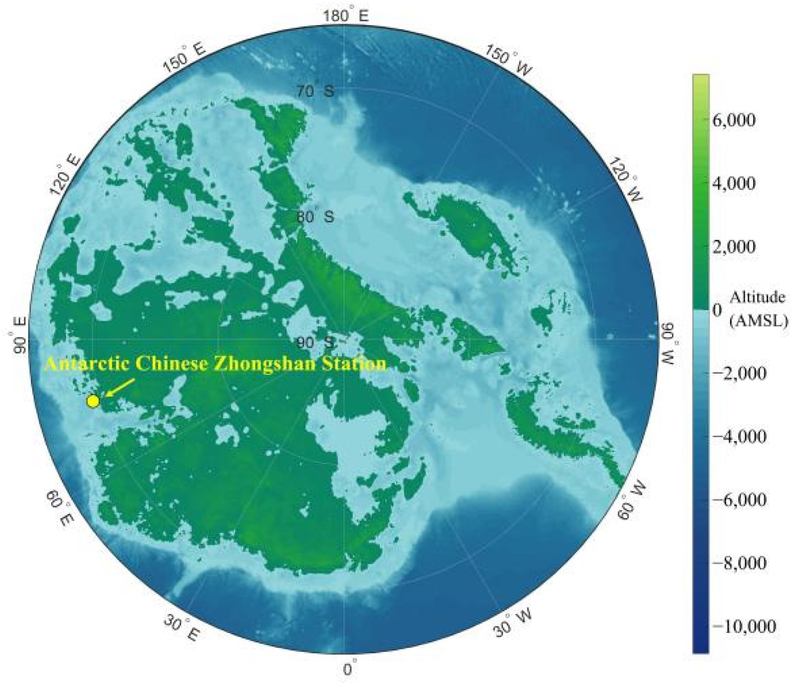
The Antarctic Chinese Zhongshan Station (76.38° E, 69.37° S, with a mean altitude of 11 m) is one of the Chinese scientific research stations in Antarctica and is located in the Lastman Massif of Southeast Antarctica, as shown in
Figure 1. The colors in
Figure 1 (from blue to green) represent different altitudes (above mean sea level [AMSL]), and the yellow dot represents the location of the Antarctic Chinese Zhongshan Station, which is close to the sea. For the Zhongshan Chinese Station in Antarctica, there are approximately two months of polar days and two months of polar nights every year. Importantly, Antarctica is excellent for observing atmospheric parameters, because there are no major atmospheric pollution sources, there are few human activities around the site, and disturbances are unlikely to occur. Solar activities can affect the atmosphere, mainly through the interaction between solar wind and geomagnetic fields. In this process, high-energy particles enter Earth’s atmosphere along magnetic field lines; therefore, the response of the atmosphere in Antarctica is more obvious and observable.
2.2. Electric Field Mill
There are various methods for measuring the AEF; commonly used methods involve ground-based rotating electric field meters, roller electric field meters, sphere-borne double-ball electric field meters, and microrocket electric field meters. In the past, the most common methods were potential probes and burning fuses, and these methods are still used by some observatories today. The most widely used method today is the electric field mill (EFM), which provides good exposure to the AEF. It usually consists of one or more electrodes that are alternately shielded and exposed to the AEF. In addition, it provides the opportunity for faster measurements with multiple options for meteorological conditions. An electric field mill is mounted outdoors, where it is well exposed to the AEF.
The AEF meters that were used for measurements in this paper are EFMs with a measurement range of ±50 kV/m, measurement accuracy < 5%, response time < 1 s, linearity < 1%, and resolution of 10 V/m. When the meter operates, the stator is fixed and grounded while the rotor rotates (the stator and rotor are two sets of similarly fan-shaped metal conductive sheets) at a uniform speed, and then the stator is periodically and alternately exposed to the environmental electric field, which generates induced charges and induced current on its fan blades. Since the atmospheric electrostatic field is a DC component, the current induced in the induction blade is a very weak signal and needs to be amplified before the AEF measurement is performed. Therefore, the preamplifier will amplify the weak current signal generated by induction, and then, through current-to-voltage conversion, amplification, filtering, signal synchronization, and rectification, the voltage signal is output, and finally, the AEF data can be obtained after processing the data arithmetic. The meter can be powered by the mains power (175–275 V), UPS power, or solar power. During measurement, the data are transmitted through a 4G network to a cloud server. Then, the local PC can download and save the data from the cloud server in real time.
2.3. Measurements
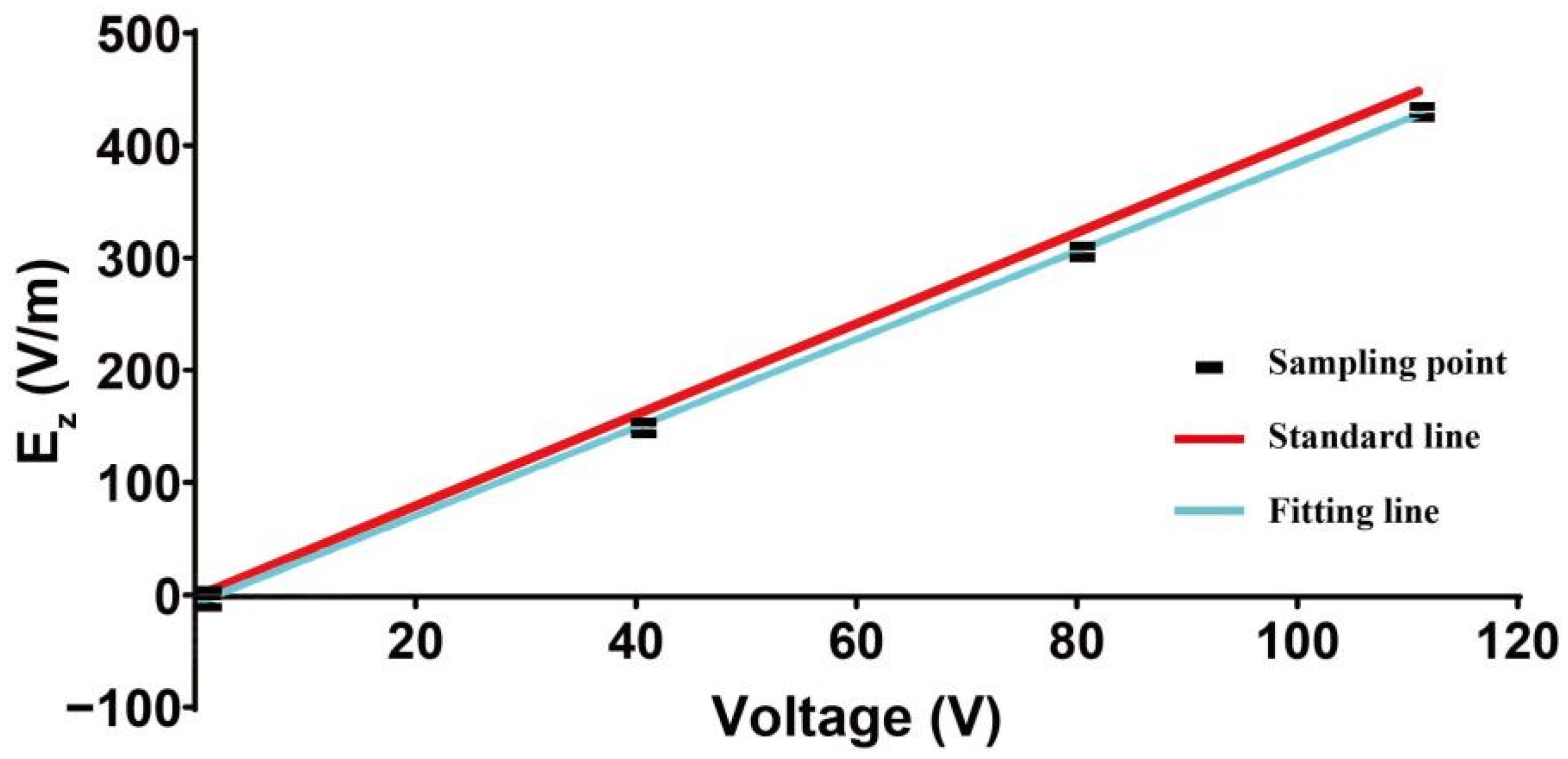
To make the results of the observation experiments more accurate and meaningful, before the Antarctic and Beijing measurement experiments were conducted, we carried out a laboratory experiment in Beijing, China. In this experiment, the researchers applied an adjustable DC voltage to two metal pole plates with a radius of 54 cm (the radius of the probe was 4.5 cm), and the height between the two plates was fixed (measured value was 24.6 cm). During the laboratory experiment, researchers set the voltage values to approximately 111, 80, 40, and 0 V to check the stability and accuracy of the probe (during the production of the probe, they completed calibration experiments). Each voltage value was retained for 5 min to determine whether the AEF value was stable.
The laboratory experimental results are shown in
Figure 2, where the horizontal axis is the voltage value, and the vertical axis represents the AEF. The red line and blue line represent the standard curve fitting curve, and the black squares indicate the sampling points obtained in
Figure 2.
Figure 2 clearly shows that the measured value does not change more than 8 V/m within 5 min for the same voltage, and the stability and linearity of this probe are excellent. However, the difference between the fitting line and the standard line is clear, which means that the theoretical value is 5–20 V/m greater than the measured value under the same voltage. This error (5–20 V/m) accounts for <5% of the standard AEF values and may be caused by the interference of the laboratory environment, the inevitable measurement system error, and the limitation of the probe measurement accuracy. These possible causes can result in the actual voltage added to the probe terminals being less than the theoretical values, or result in the actual measured voltage being lower, so that the measured values of AEF are 5–20 V/m lower than the theoretical values.
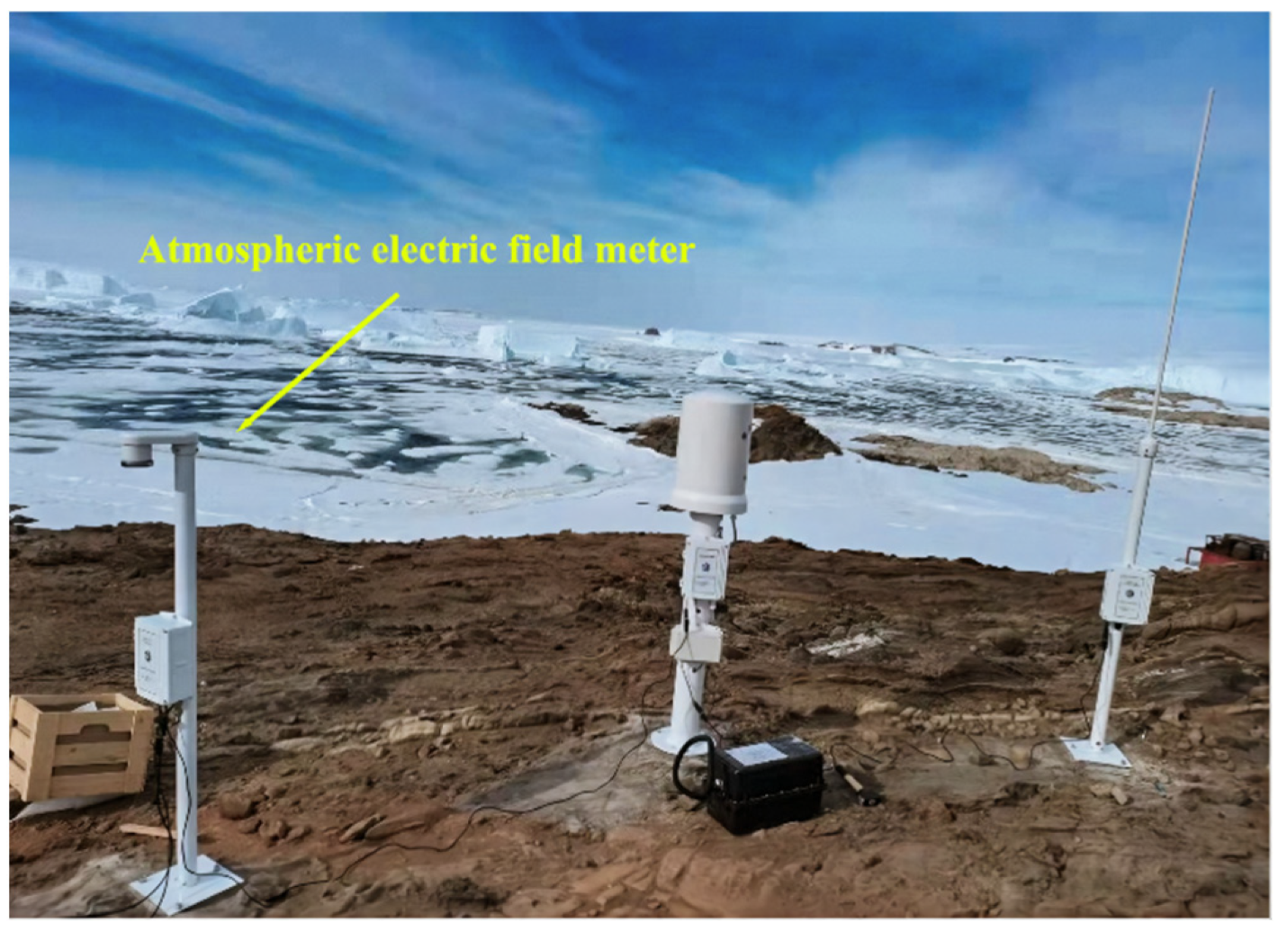
The topographic relief, buildings or communication base stations and other protrusions can affect the distribution of the AEF, making the atmospheric equipotential surface a changing surface, which in turn affects the measurement error of the AEF. Therefore, in the practical application of an AEF meter, it is generally required that it be installed in a certain elevation range where there are no protrusions, trees, signal towers, sharp objects, human activities, or other sources of interference. A photo of the observation scene at the Antarctic Chinese Zhongshan Station is shown in
Figure 3. The yellow arrow points to the EFM, while the other two instruments are used to observe other relevant physical parameters. The EFM is constructed with the probe at the top, which contains the motor, stator, rotor, and circuitry, and the electrical box in the middle, which contains the power supply and data processing and data transmission equipment. The instrument is powered by main electricity and will not be interrupted by weather or external factors. The height of the mast is 1.5 m, and it serves as a support. This mast is made in bulk by the manufacturer, and its exterior is fully insulated and does not interfere with the measured value of the AEF. Due to the impact of the station, it must be placed relatively close to snow, ice, and water sources, which can cause unavoidable interference to the AEF measurements [
44]. The area surrounding the AEF meter is empty, with no high buildings, sharp objects, grass or trees, or other sources of interference except for the other two nearby instruments. Therefore, this location is a long-term observatory station for studying the differences in the atmospheric electric environment at different latitudes and the interaction of solar activity with the Earth’s near-surface atmosphere.
2.4. Criteria of Fair Weather
For the study of fair-weather AEFs, having a clear definition of fair weather that incorporates clear quantitative criteria to uniquely determine and classify fair days is necessary. However, fair weather criteria are highly subjective from place to place [
45] and are determined based on atmospheric conditions; thus, fair days were defined in this reference with the following detailed definitions: (1) the visual range should be 2 to 5 km or greater, and the relative humidity should be less than 95%; (2) there should be no low stratus clouds and negligible cumuliform clouds; and (3) the wind speed at 10 m should be less than 8 m/s. In contrast, Latha [
46] defined fair days as having a cloud volume of less than 3/8, a wind speed of less than 4 m/s, and no precipitation. Similar definitions have been put forward by other scholars. Deshpande and Kamra [
43] considered fair weather to exist when snow and low clouds are absent, high clouds are characterized by fewer than three oktas, and the wind speed is less than 10 m/s. Among the most recent studies mentioned in this paper, the researchers define fair days as follows: (1) maximum relative humidity < 95%; (2) a visual range ≥ 5 km; (3) an average wind speed at 10–12 m less than 9 m/s; and (4) hourly average AEF values (HAEFs) ≥ 0 V/m.
3. Results
Using the website Rp5 (
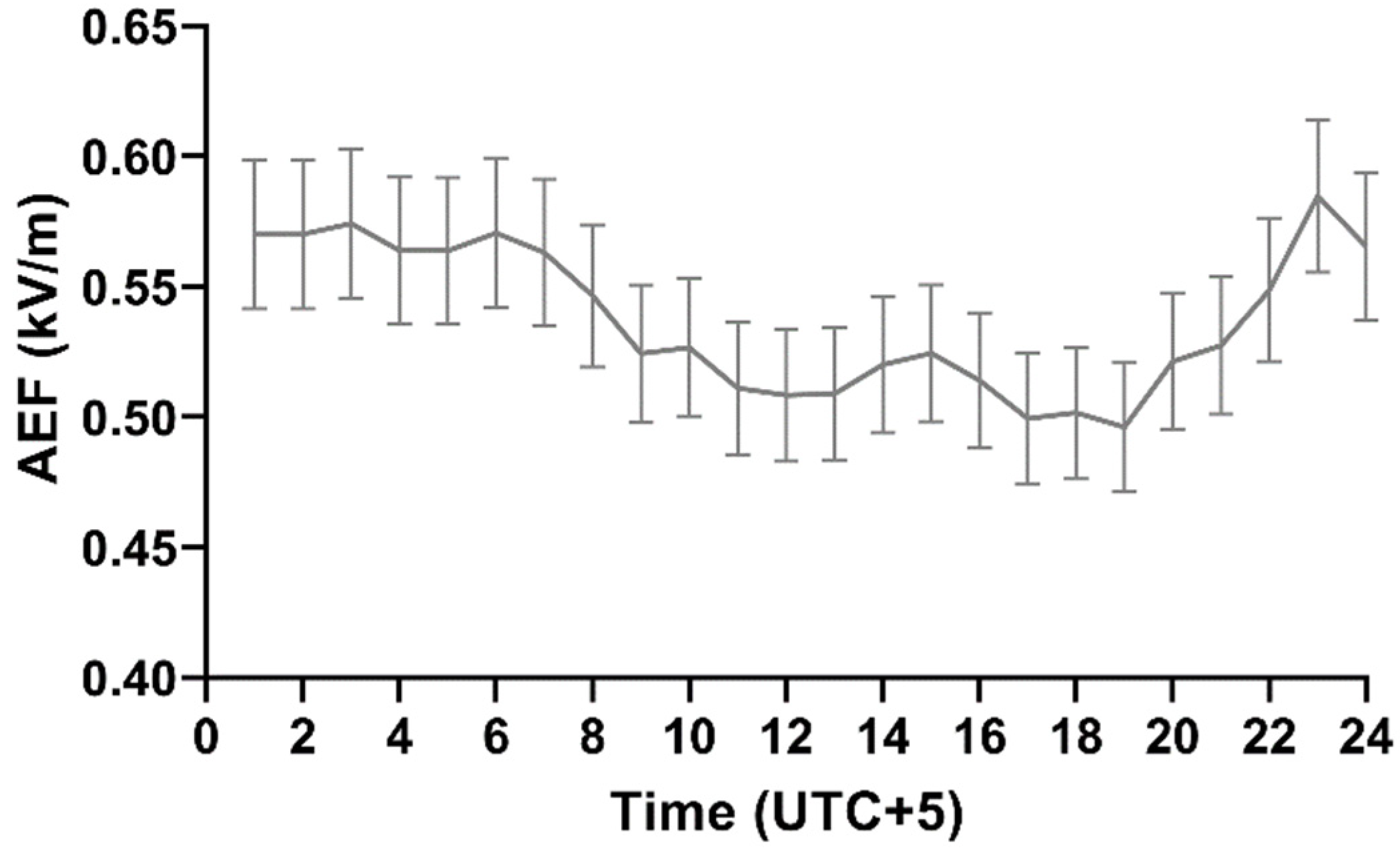
https://rp5.ru (accessed on: 12 July 2022)), the researchers obtained meteorological data (including relative humidity, temperature, atmospheric pressure, visual range, and wind speed) from the Zhongshan Chinese Station, Antarctica. Notably, temperature is the atmospheric temperature at 2 m above ground level (℃), wind speed is the average wind speed at 10–12 m within 10 min of observation (m/s), relative humidity is measured at 2 m above the ground (%), atmospheric pressure is the atmospheric pressure at the level of the weather station (mmHg), and visibility is the horizontal visibility (km). Many researchers have shown that space weather can have an effect on the AEF; therefore, we should exclude days of magnetic storms with Dst indices less than −50 nT, indicating moderate and large storms. Finally, 40 days were selected as fair-weather days during the 5-month measurement period (1 March–1 August 2022); the hourly average curves of these 40 fair days are shown in
Figure 4. The horizontal coordinate indicates local time (UTC+5), and the vertical coordinate is the AEF in
Figure 4. The black curve indicates HAEFs for each hour of the 40 fair-weather days, and error bars represent the corresponding standard deviations (±5% of measured values). The following summary based on
Figure 4 can be developed: (1) most of the HAEFs are in the range of 0.5–0.6 kV/m; (2) the average curve as a whole is a “single-peak, single-valley” curve; and (3) the maximum peak value is 0.58 kV/m at 23:00, and the minimum valley is 0.50 kV/m at 19:00.
Earth’s conductivity and the ionospheric conductivity are so high as to act as equipotential points. The current density is given by Ohm’s Law, J
z = V
i/R, where R is the whole-column resistance from the surface to the ionosphere at that location and time and is essentially constant during the day. Therefore, the conduction current (J
z) in the atmosphere varies with time during each day, as the overhead ionospheric potential (V
i) varies, forming the well-known ‘Carnegie Curve’. At a specific location and time, the AEF is inversely proportional to the atmospheric conductivity, while atmospheric conductivity is positively correlated with small ion concentrations and is inversely proportional to the concentration of large ions in the atmosphere. When the aerosol concentration increases, the large ion concentration increases, which leads to a decrease in the atmospheric conductivity and an increase in the AEF. Therefore, there is a positive correlation between near-surface AEFs and aerosol concentrations [
47]. Then, we changed the view to observe the details of the orange curve. In the morning, aerosols gathered near the ground, which led to an increase in the aerosol concentration and then an increase in the AEF. From 6:00 to 19:00, thermal convection and turbulent vertical transport were active because of solar radiation. Moreover, aerosols were transported upward, and their concentrations near the surface continuously decreased. Subsequently, the near-surface AEF decreased to a valley value. Finally, from 19:00 to the early morning of the next day, the atmosphere stabilized, the aerosol concentration increased, and the AEF slowly increased and stabilized.
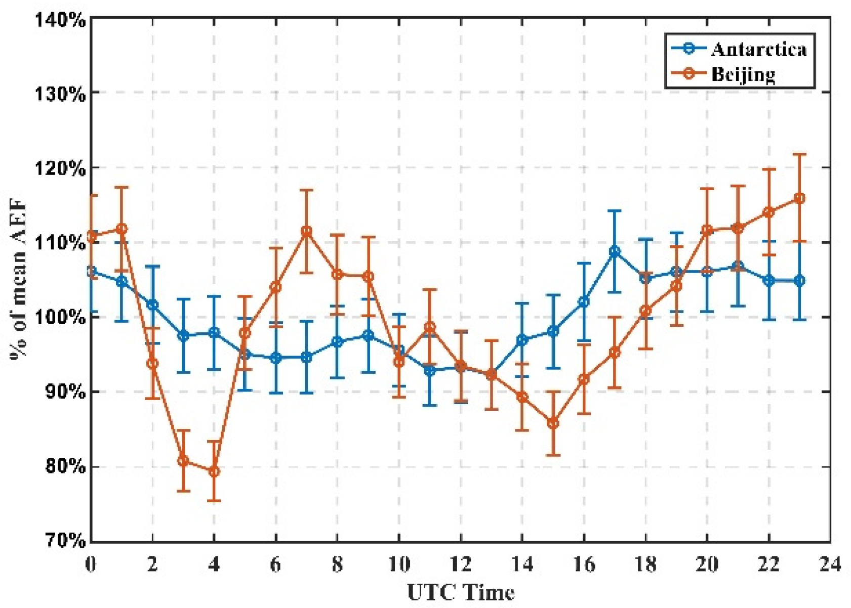
To make a comparison, using the same method, the researchers conducted long-term observations at the Thirteen Hill Station in Changping, Beijing, China (116.23° E, 40.25° N, with a mean altitude of 198 m). In the AEF observation experiment at Beijing Thirteen Hill Station, the researchers use the EFM as described above. The instrument is grounded well and mounted on top of a 2.5 m high cottage with a roof that is sufficiently wide and flat, surrounded by no grass or other protruding objects, with the nearest trees more than 10 m away and no shading; thus, these environmental factors do not affect the near-surface AEF measurements. Sunlight is plentiful here, so the EFM is powered by solar energy, and the support mast and other instrument details are the same as those used in Antarctica. After using a similar method as described above and a fair-weather criterion, the authors selected 37 fair days from a period of 5 months, as detailed above (1 March–1 August 2022). These two different hourly average curves are shown in
Figure 5. The vertical coordinate is the percentage of each AEF value/mean AEF (%), and the horizontal coordinate indicates the time in UT. Then, the blue line shows the percentage curve of daily variation for Antarctica, while the red line shows the percentage curve of daily variation for Beijing. The error bar corresponds to the standard deviation of the instrument. For the average daily variation curve in Beijing, the curve is a “double-peak, double-valley” curve, with the initial peak value of 112% of the mean AEF (0.19 kV/m) at 7:00 UT and the other peak value of 116% of the mean AEF (0.19 kV/m) at 24:00 UT, the minimum valley value of 79% of the mean AEF (0.13 kV/m) at 4:00 UT and the other valley value of 86% of the mean AEF (0.14 kV/m) at 15:00 UT. From 4:00 UT to 7:00 UT, the aerosols gathered near the ground. Additionally, the aerosol concentration and AEF increased, with the maximum peak appearing at approximately 7:00 UT. From 7:00 UT to 15:00 UT, due to strong solar radiation, the vertical transport of thermal convection and turbulence was active, aerosols were continuously transported upward from near the ground, the near-surface aerosol concentration continuously decreased, and the near-surface AEF reached the minimum valley at 15:00 UT. Then, from 15:00 UT to 24:00 UT, the upper aerosol concentration was greater than that near the ground. Due to atmospheric pressure, aerosols were vertically transported, and the aerosol concentration near the ground again increased. Then, the AEF also increased, reaching another peak at 24:00 UT. From 24:00 UT to 4:00 UT, the atmosphere gradually stabilized, and the aerosol concentration decreased. In addition, the AEF decreased to another valley at 4:00 UT.
4. Discussion
By comparing the two different curves in
Figure 5, their differences can be summarized in the following discussion. (1) The characteristics of the average daily variation curves in Antarctica and Beijing are obviously different; the daily variation curve of Antarctica changes by 17% of the mean AEF, while the curve of Beijing changes by 37%, and the daily variation of Beijing fluctuates even more. Their curves are represented by the following two different types: the curve in Antarctica is “single peak, single valley” on the whole, while the curve in Beijing is characterized by “double peaks, double valleys,” which are mainly determined by the local geological conditions and environmental factors. The composition and content of radioactive substances vary under the crust in different regions, and they affect atmospheric ionization, which in turn affects the state of space charge density distribution and thus disturbs the AEF. Antarctica is remote, sparsely populated, and far from aerosol sources, while Beijing is densely populated. Therefore, the curves in these regions take on two different shapes, and the average daily variation curve in Beijing is more complicated than that in Antarctica. (2) There is a significant difference in the time of peak and valley values of the two curves because of the different longitudes, which result in different sunrise and sunset times in the two regions. The sunrise and sunset times determine the intensity and time of the vertical transport of aerosols, which in turn affects the peak and valley times of the AEF daily variation curves. (3) In addition, the average fair-weather AEF value in Antarctica was 0.54 kV/m, while it was 0.17 kV/m in Beijing. Not only is the value in Antarctica 0.37 kV/m higher than that in Beijing, but this value significantly exceeds the observations made by other researchers. The authors attribute the reasons for this difference as the following: (i) there is less precipitation and lower temperature in Antarctica, and the area around the instrument is mostly ice and snow, and these conditions resulted in fewer radioactive substances and fewer charged small ions in Antarctica. (ii) The latitudinal difference between Antarctica and Beijing is a factor, because there is a certain horizontal potential difference at the bottom of the ionosphere between the polar region and middle or low latitudes. (iii) The Antarctic Chinese Zhongshan Station is located in the south auroral zone, so the ionospheric potential may be influenced by magnetospheric currents, which raises the ionospheric potential at dawn by approximately 25 kV during low magnetic activity, while lowering the nighttime ionospheric potential by approximately 25 kV. This effect would cause the AEF values in the morning to be higher and the those in the evening to be lower in Antarctica. (iv) Due to the location limitations of the Antarctic Chinese Zhongshan Station, the EFM in Antarctica is close to snow, ice, and water sources. This increases the water vapor molecules around the EFM, causing many light ions to attach to the water molecules and become heavy ions, a process that reduces the atmospheric conductivity near the ground. (v) The wind speed at the Antarctic Chinese Zhongshan Station was relatively high, with an average of more than 6 m/s at 52% of the moments, which is a much higher percentage than normal weather. High winds can carry ions of particulate matter through the air and change the distribution of space charge, which could have disturbed the AEF values in Antarctica.
There are many inevitable and reasonable errors in the experimental process. First, the EFM is a method of generating induced charges and weak current through the rotation of the stator and rotor, which can be easily disturbed by environmental factors. Then, the EFM has a certain measurement accuracy, resolution, zero stability, and linearity due to the limitation of circuit components. The stator and rotor of the EFM may leave ice or dust particles, and these dust particles may be charged, which leads to the AEF observed by the EFM not being the AEF in the atmosphere, and this can lead to experimental errors. In addition, unstable supply voltage leads to unstable rotation between the stator and rotor, which also leads to unavoidable experimental errors.
The limitations of this study are (1) the instrument will degrade over a long period of continuous operation and produce measurement errors, and (2) the requirement for human analysis of the data and the lack of automated algorithms. Next the researchers will try to use new technologies and AI algorithms for future improvements to electric field measurements at the Zhongshan Chinese Station in Antarctica, which will make the device require low energy and work without human intervention.
5. Conclusions
In summary, to study the baseline variability characteristics of the near-surface electrical environment in the Antarctic region, the authors conducted long-term observation experiments at the Zhongshan Chinese Station using EFM. Before the observation experiments, the authors performed laboratory measurements to ensure the accuracy of the observation experiment, even though the EFM had been rigorously calibrated during production. After defining the criteria for clear days and excluding the interference of magnetic storms, 40 fair-weather days were selected between 1 March–1 August 2022, at Zhongshan Station in Antarctica. Then, the average curve of the AEF daily variations of the 40 fair-weather days was plotted and compared with the curve during the same period in Beijing. The curve of the AEF in Antarctica has a “single peak, single valley,”, which is different from the “double-peak, double-valley” curve in Beijing. As the Antarctic region is much less densely populated than Beijing and far from aerosol sources, the curves in these regions are of two different types, and the daily variation in the AEF in Antarctica is simpler than that in Beijing. In addition, the difference in sunrise and sunset times causes the peak and valley to appear at different times. Finally, although the EFMs at the Antarctic Chinese Zhongshan Station and Beijing Thirteen Hill Station were produced by the same facility, the average fair-weather AEF value in Antarctica is significantly greater than that in Beijing by 0.37 kV/m, and the AEF values in Antarctica exceed the observations reported by other researchers. The authors attribute the reasons to the following: (i) less precipitation, fewer radioactive substances, and fewer charged small ions in Antarctica; (ii) certain horizontal potential difference between Antarctica and Beijing and other regions; (iii) variation in ionospheric potential; (iv) the proximity of the EFM in Antarctica to water sources; (v) differences in wind speed. Taking advantage of the fact that the Zhongshan Chinese Station in Antarctica is at a high latitude, additional research on the relationships between the AEF and solar activities and geological conditions will be conducted.

 ,
, 


