
A Robust H∞ Application for Motor-Link Control Systems of Industrial Manipulators

1
Dipartimento di Elettronica e Telecomunicazioni, Politecnico di Torino, Corso Duca degli Abruzzi, 24, 10129 Torino, Italy
2
COMAU SpA, Via Rivalta 30, 10095 Grugliasco, Italy
*
Author to whom correspondence should be addressed.
Appl. Sci. 2022, 12(17), 8890; https://doi.org/10.3390/app12178890
Submission received: 22 June 2022
/
Revised: 30 August 2022
/
Accepted: 31 August 2022
/
Published: 5 September 2022
(This article belongs to the Special Issue Robots Dynamics: Application and Control)
Abstract
: control approaches are widely investigated in various application fields and in the robotics area, too, for their robustness properties. However, they are still rarely adopted in the industrial context for the control of robot manipulators, mainly due to the lack of predefined procedures to build weighting functions able to automatically guarantee the fulfillment of the control objectives. This paper reports the first results of an academic–industrial research activity aimed at investigating the adoption of an approach in the control software architecture of industrial manipulators, equipped with standard sensors on the motor side only. The design of the control system for a single-axis of an industrial manipulator is developed, showing that the construction of the weighting functions according to standard procedures can provide a satisfying behavior only on the motor side, leaving unacceptable oscillations of the link. A different procedure is then developed for the definition of the weighting functions with the specific aim of eliminating the possible vibrations of the mechanical structure. The proposed new form of such functions, including the main dynamic characteristics of the plant, ensures a robust, satisfying behavior on both the motor and the link side, as proven by simulation and experimental results.
1. Introduction
In recent years, thanks to the persistent growth of automation, the employment of industrial robots in different applications keeps increasing. Moreover, the demands on their performances are beginning to be much more accurate and meticulous. In addition, there is also the desire of reducing costs, improving safety, and reaching high-speed and precision in movements. This incessant progress confers to the control research area a remarkable focus, it having a direct responsibility of the manipulator’s behavior.
The robots of the latest generation have lower weight and lower mechanical stiffness, and hence they may suffer more frequently from significant vibration problems, especially when operating at high-speed conditions. Vibrations in mechanical structures constitute a common criticality in the robotic field, which must be robustly handled by the control system.
The control system can easily counteract the effects of vibrations on the mechanical arm if some measures of them are included in the closed-loop architecture as additional inputs. This happens if some further sensor, for example, a link gyroscope, is added to the system, capturing these events and feeding the back to the controller. Some solutions have been recently proposed in literature exploiting the usage of additional sensors, such as in [1], where a robust control scheme is developed and applied to the base joints of an industrial KUKA robot, equipped with secondary encoders, and in [2], where vibration control is addressed by means of multi-modal, time-varying input shaping based on the identification of the dynamic map of the robot using accelerometers. The drawback of these solutions is that such additional sensors are not generally available for all the industrial robots. In most cases, the measurements come from sensors installed on the motor that do not give information about the end-effector behavior. Here, the action of the control system is much more complex, since it has to balance out possible link excitations without directly knowing them.
Our main goal, then, will just be to guarantee satisfying responses from both the motor and link by only having motor measures available.
Through the years, many types of robot-control systems have been exploited. The state-of-the-art recognizes the following control systems among the most important ones: the computed-torque control and the joint-space control, including PD control, PID control, Inverse Dynamics control, and Lyapunov-based control. However, since the dynamics of robots are highly non-linear and contain uncertain parameters, high performance is not often achieved by means of this class of algorithms. In particular, PI or PID controls have issues in parameter tuning, and because of their simple structure, the attainment of proper achievements is usually a slow process that can involve many iterations, especially for several Degrees of Freedom (DOFs) manipulators comprising high non-linearities and couplings.
Because of this, industries are particularly interested in investigating the application of control methodologies assuring robust properties in front of nonlinear and complex behaviors in the presence of possible vibration problems at high velocity, possibly avoiding too complex or too specific approaches. In the literature, the interested reader can find various ad-hoc solutions to address the vibration suppression problem, for example, through preshaping input trajectories, as in [3], or by means of an online real-time path compensation system based on a laser tracker, as in [4]. In this context, control finds space. The problem is that, despite its relevance in control literature, currently, its application appears to be still limited in the manufacturing world.
In order to overcome application difficulties, over time, many researchers have investigated this topic by presenting various types of control implementations.
In 2012, a study on the development of an controller with LMI region schemes for trajectory tracking and vibration control of a planar single-flexible link was proposed in [5].
In 2013, the implementation of two controllers by using both the Loop--shaping approach and the Mixed one has been presented in [6]. Model order reduction of controllers is also discussed, and a comparison between the developed methodology and the canonical PID control shows the advantages of using robust approaches.
In 2015, a study about a different implementation of the standard theory was developed in [7]. Here, the key idea is to add to the original control law an auxiliary PID input that attenuates the deviation due to modeling uncertainties and unknown disturbances.
In 2016, the control of a non-linear robotic manipulator by using the technique was discussed in [8]. The control is also compared to a Model Predictive controller, where the optimization of the control action is derived by considering past and future behaviors of the system under analysis.
In 2017, two non-linear control schemes for multi-DOF robotic manipulators were proposed in [9]. The authors formulated the control problem as a min-max differential problem, and they designed the controller through the solution of a Riccati equation.
In 2018, an adapting computed-torque controller was proposed in [10], requiring few parameters to be set. This is a very important result, since it allows one to realize and analyze the entire architecture in an easy way. Moreover, the controller does not need any specific initial information, and it automatically adapts to the real system dynamics. The technique is used as proof of the robustness of the proposed controller, whose validity is confirmed by experimental results for a 3DOF and a 7DOF robot manipulator.
The algorithm is also used to achieve high-precision tracking performance in [11]. On the basis of theoretical results on robust finite-time stability for uncertain systems, a robust controller is developed by means of the back-stepping approach, achieving high precision, strong robustness, and fast response. Simulations and experimental results confirm the effectiveness of the proposed controller.
More recently, a work emphasizing the design of robust control for a 3DOF robotic manipulator under uncertainties was carried out in [12]. The synthesis, under which the controller was developed, is compared with PID, proving how the controller achieved better noise rejection, disturbance rejection, performance, and stability robustness characteristics.
A new and interesting approach combining identification and control design for controlling multiple-link elastic joint robots in the presence of model uncertainties is developed in [13]. The controller has two degrees of freedom, and it is able to withstand uncertainties and variations in model parameters as well as to track reference trajectories. The last aspect is simplified by the presence of a feed-forward action that anticipates the possible future trajectories.
In [14], the robust control of robot manipulators is investigated comparing the performances achieved by robust PID controllers, tuned through the Quantitative Feedback Theory (QFT) approach, and the ones provided by the application of control, by adopting a standard procedure for the design of the weighting functions. The results achieved by the first control solution seem better, but it must be underlined that only simulation tests were performed, without taking into account the different behavior on the motor and the link side that occurs in practice.
Furthermore, very recent results on the application of robust control techniques were published in 2021, but they do not seem mature for an actual industrial application yet. For example, in [15], preliminary results are provided for a robust control approach for multi-DOF manipulators, performing tasks requiring frequent interactions with the environment; in [16], a robust discontinuous controller algorithm is proposed for a 5DOF laboratory robot, whereas, in [17], an interesting adaptive proportional integral robust control scheme is developed for n-link robotic manipulators with model uncertainties and time-varying disturbances, but only simulation results for a two-link robot are available.
The approach is rarely applied in the industrial context because there are not predefined procedures to build weighting functions able to automatically guarantee the fulfillment of the control specifications. The design of the weighting functions is a slow iterative process that can take a long time, and this is not acceptable in an industrial reality that asks for valid results in a short time. Even if the research world counts many studies referring to the method, as previously discussed, most research is focused on the advantages of its robustness properties, without guiding the reader in the development of the implementation steps. In the meantime, the most frequently implemented solutions still rely on control schemes of PID type, in which techniques such as Linear Quadratic Theory (LQT) are applied to achieve optimal tracking results (see [18] and the references therein for insight into LQT and the generalized PID controllers thus derived, denoted as PID).
This paper reports the results of an academic–industrial research activity, carried out in collaboration between Politecnico di Torino and COMAU S.p.A. The goal is to investigate the adoption of approaches in the control software architecture of industrial manipulators, providing a proof-of-concept demonstration potentially useful as a basis for a concrete and complete robust control scheme alternatives to PID or generalized PID ones. The design of the control system for a single axis of a 6DOF manipulator is presented, describing all the steps that have to be fulfilled to reach satisfying time results, with a particular attention to the construction of two weighting functions summarizing the frequency requirements of the system. No specific assumption is made on the trajectories that will be applied, since in practice they are provided by the internal jerk bounded reference trajectory generator of the robot constructor, i.e., COMAU in our case.
Our target to is to prove the potentiality of the application of the complex theory to a much more complex world, which is the robotic one, where systems are not linear and where the models are continually affected by external disturbances. It is interesting to highlight that the application of robust control techniques have been recently investigated in other areas of the robotic world, such as in [19], where resilient interval consensus problems for continuous-time, time-varying, multi-agent systems are addressed. In this paper, starting from a realistic case, it will be shown how weighting functions defined according to standard procedures are not suitable for controlling the considered plant. General guidelines for the design of new weighting functions incorporating plant dynamic characteristics are exploited in order to obtain a control system responsive to both motor vibration, captured by sensors (as in the standard industrial configuration) and link vibration, on which no information is available.
Matlab has been adopted as computing environment, using the Simulink toolbox to carry out simulation tests before moving to experimental tests on a real robot, whose preliminary but significant results are reported and discussed.
The paper is organized as follows: Section 2 illustrates the basics of the approach, with a particular focus on the definition of the involved weighting functions. Section 3 is fully devoted to the development of an control system for an industrial Comau manipulator axis. General control requirements are derived, and the Linear Matrix Inequality (LMI) technique is adopted to determine the controller. The simulation of motor and link responses shows the inability of the standard design procedure to damp link oscillations, due to the plant dynamics’ cancellation within the control action, as discussed in Section 4. A new implementation approach is then proposed in Section 5, based on different definitions of the weighting functions, leading to robust and satisfying behavior of both the motor and the link. Section 6 reports experimental results that confirm the effectiveness of the proposed solution. Section 7 finally draws some conclusions and sketches possible future works.
2. Control Approach Basics
2.1. General Outlines
represents one of the most known robust control techniques. It minimizes the effects of high disturbances and model uncertainties and it ensures system stability in the presence of variations in parameters and operating conditions.
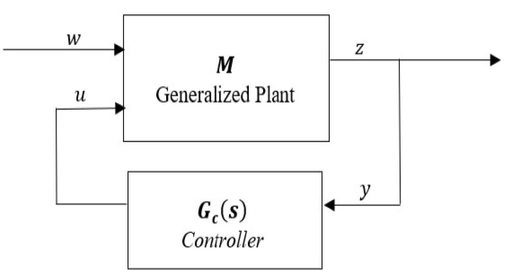
The actors that play a fundamental role in the control structure (Figure 1) are the generalized plant M and the controller, whose derivation depicts the purpose of the design.
The generalized plant M includes the nominal plant, the actuators, the sensors, and two weighting functions taking into account all the design requirements. Its inputs, w, represent references, disturbances, sensor noises, while its outputs, z, represent the signals that have to be controlled and the plant outputs. Both the plant and the controller are assumed to be rational and proper functions. Furthermore, the state-space models of M and are assumed to be available and their realizations are assumed to be stabilizable and detectable [20].
From a theoretical point of view, developing an control system means designing a controller that minimizes the norm of the closed-loop transfer matrix :
The controller is chosen among a set of controllers that make the system internally stable () as the one that produces a signal u that counteracts the influence of w and z [20], minimizing the norm .
It must be underlined that the solution of (1) is not unique in general. In addition, the computation of an optimal controller is not easy, as well as not always requested. Rather, it is preferable to find controllers that are very close to the optimal ones.
This leads to the class of sub-optimal control problems: the controller is chosen as the one that stabilizes the closed-loop system and achieves , a non-negative number which represents the best performance [21].
There are many ways to solve the optimization problem in (1) and to derive the controller transfer function. Here, the synthesis will be accomplished by means of an LMI-based technique, exploiting in particular the LMI Matlab Toolbox.
2.2. The Closed-Loop Control Architecture
The accuracy of the movements performed by a robotic arm is estimated by means of the analysis of velocity and position measurements of each axis of the kinematic chain.
A typical industrial manipulator has 6DOFs. The most common control architectures can be regrouped as follows:
- In the first case, the manipulator is considered as a unique multi-DOF system and a completely centralized controller is implemented.
- In the second case, six independent controllers, each one linked to a single axis of the structure, are developed. In the end, they are synchronized to let them operate as a single one.
This paper is focused on the second kind of control architecture, dealing with a single axis of a 6DOF manipulator, considered as a single DOF system.
Since industrial manipulators are generally not equipped with link gyroscopes, the control is realized at the motor side but with the purpose of reaching satisfying performances for the link motion.
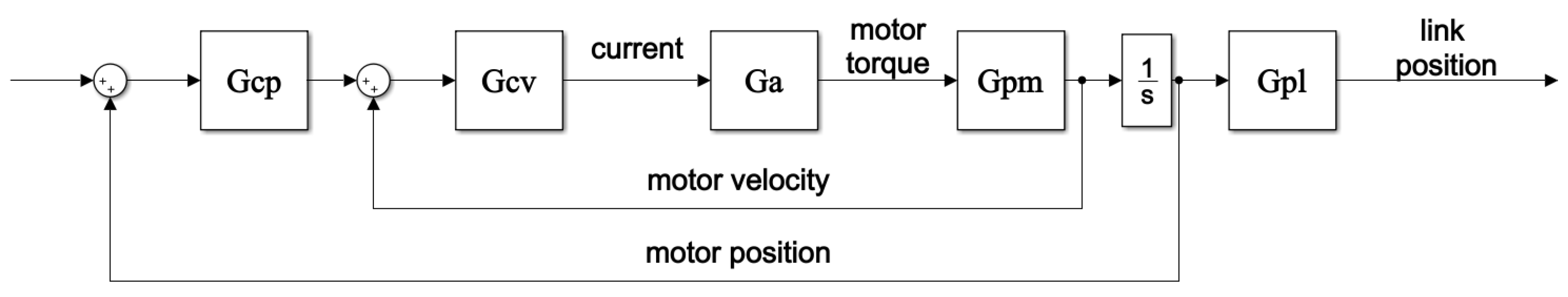
The control architecture is composed by two nested loops (Figure 2), in order to split up the overall complex motion control problem into two smaller ones, according to the “divide et impera” technique: the inner one is a velocity loop, in which a velocity controller is applied based on the motor velocity feedback, whereas the outer one is a position loop, in which a position controller based on the motor position feedback is applied to the velocity-controlled system.
It is worth to be noted that the control architecture in Figure 2 includes neither a current loop nor any feed-forward term.
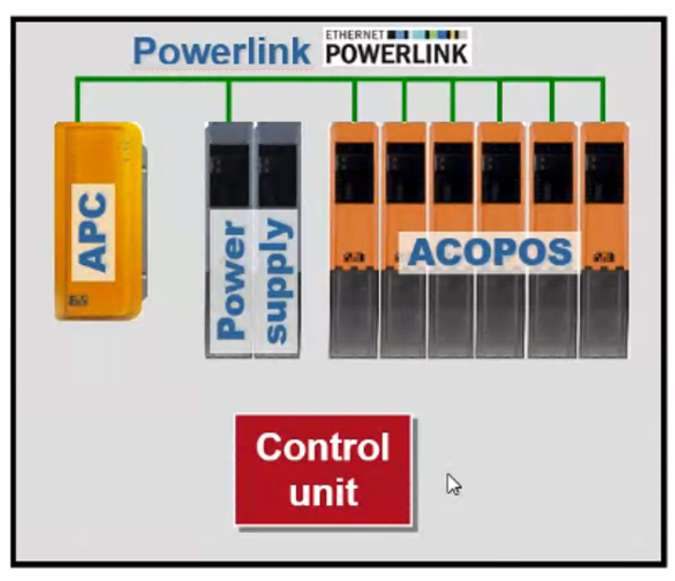
With reference to the actual control software architecture of industrial robots, the current loop is assumed to be directly included in the servo-system implemented on board, i.e., the APOCOS by B&R for COMAU robots (Figure 3), whereas the velocity and position loops (and in general any specific control scheme adopted) are implemented in the Automation PC (APC) component.
In this kind of control architecture, feed-forward terms are not always strictly required, thanks to the good behavior offered by the system when controlling a base industrial arm axis in a specific inertia condition, such as in the considered case. In particular:
- A velocity feed-forward is generally used to synchronize all the axes of the manipulator. It is computed starting from a prefixed delay that the controllers of all the mechanical bodies of the structures have to meet. Such a term has not been included in the considered scheme for the sake of simplicity, since the goal here is to prove the effectiveness of the control applied to a single axis of the robot, working as if it were its only component.
- An acceleration feed-forward term could be added to compensate a possible unacceptable overshoot; in addition, it is a powerful instrument to make the step response invariant in the presence of varying load inertia conditions. The considered case is relative to the analysis of the behavior of a robot moving in a single inertia condition, and as it will be shown in the remainder of the paper, no high overshoot occurs requiring an additional damping action.
The adoption of the approach in the design of both controllers will enhance the stability robustness of the controlled system because possible limits or weakness of the inner system can be overcome by the outer one.
In Figure 2, is the plant model used for the velocity loop. It can be expressed as a third-order transfer function, relating the motor torque and the motor velocity as:
where:
- is the motor inertia moment;
- is the link inertia moment;
- is the gear transmission;
- K is the stiffness;
- is the damping factor;
- is the motor viscous friction;
- is the link viscous friction.
The position control loop derives from the velocity one. In this case, the plant is given by the closed-loop velocity function with the addition of the integral term that generates position from velocity.
In Figure 2, and are, respectively, the velocity and position controller transfer functions, which will be developed in the next sections. describes the actuator: it converts the current into the motor torque, representing the velocity plant input; in our case, it simply corresponds to a constant parameter . is the link model transfer function relating the motor position to the link one, as:
where the physical parameters , , , K, are defined as for the plant model (2).
2.3. The Weighting Functions
In addition to the indispensable stability requirement, a feedback control system must guarantee adequate performances as regards reference tracking, disturbance rejection, sensor noise attenuation, control sensitivity minimization, and robustness to modeling errors.
All these requirements can be depicted by means of proper definitions of the sensitivity function and complementary sensitivity function .
Ideally, both functions should be kept as small as possible in wide frequency ranges to accomplish all the requirements, but since and are such that , it is not possible to simultaneously keep them small in any frequency region.
Since reference trajectories and disturbances are usually low-frequency signals, while sensor noise and modeling errors are concentrated at high frequencies, a convenient trade-off is achieved making small at low frequencies and at high ones.
The algorithm uses weighting functions to summarize the design requirements and the open- and closed-loop response characteristics. and are the mirrors of and , respectively. They are rational, stable, and minimum-phase transfer functions. The critical issue of this kind of approach is that most of times they are formulated by using trial and error procedures, which slow down the design procedure and do not always guarantee optimal results.
Since there is not a predefined, automatic way to build them, in the literature, several different formulations can be found, and their suitability strongly depends on the particular application field.
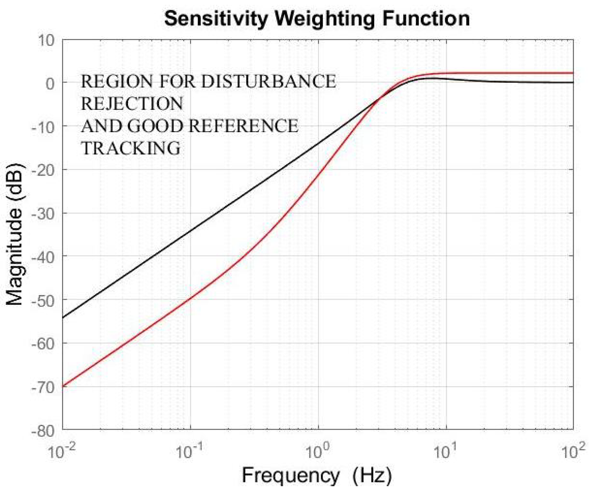
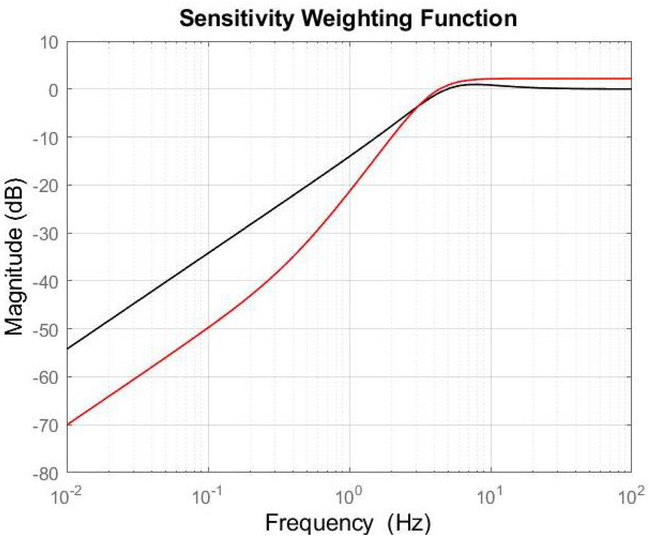
A possible choice for , e.g., following the guidelines in [20], is:
in which both the numerator and the denominator are given by Butterworth polynomials, to obtain a frequency response as flat as possible in the bandwidth of interest (Figure 4).
In (4), the coefficients a, , and have to be properly defined in order to fulfill the frequency specifications. Selecting all the parameters by using a trial and error technique is not efficient, since it might require several iterations to reach a function form as close as possible to the desired one. For this reason, only the first two parameters are actually chosen by trial and error, while is determined from them imposing the following two conditions:
where a is a constant parameter that has to be chosen to obtain a weighting function resembling the sensitivity one, and
where is the maximum allowed resonant peak of . The last coefficient in is then derived by imposing:
thus obtaining:
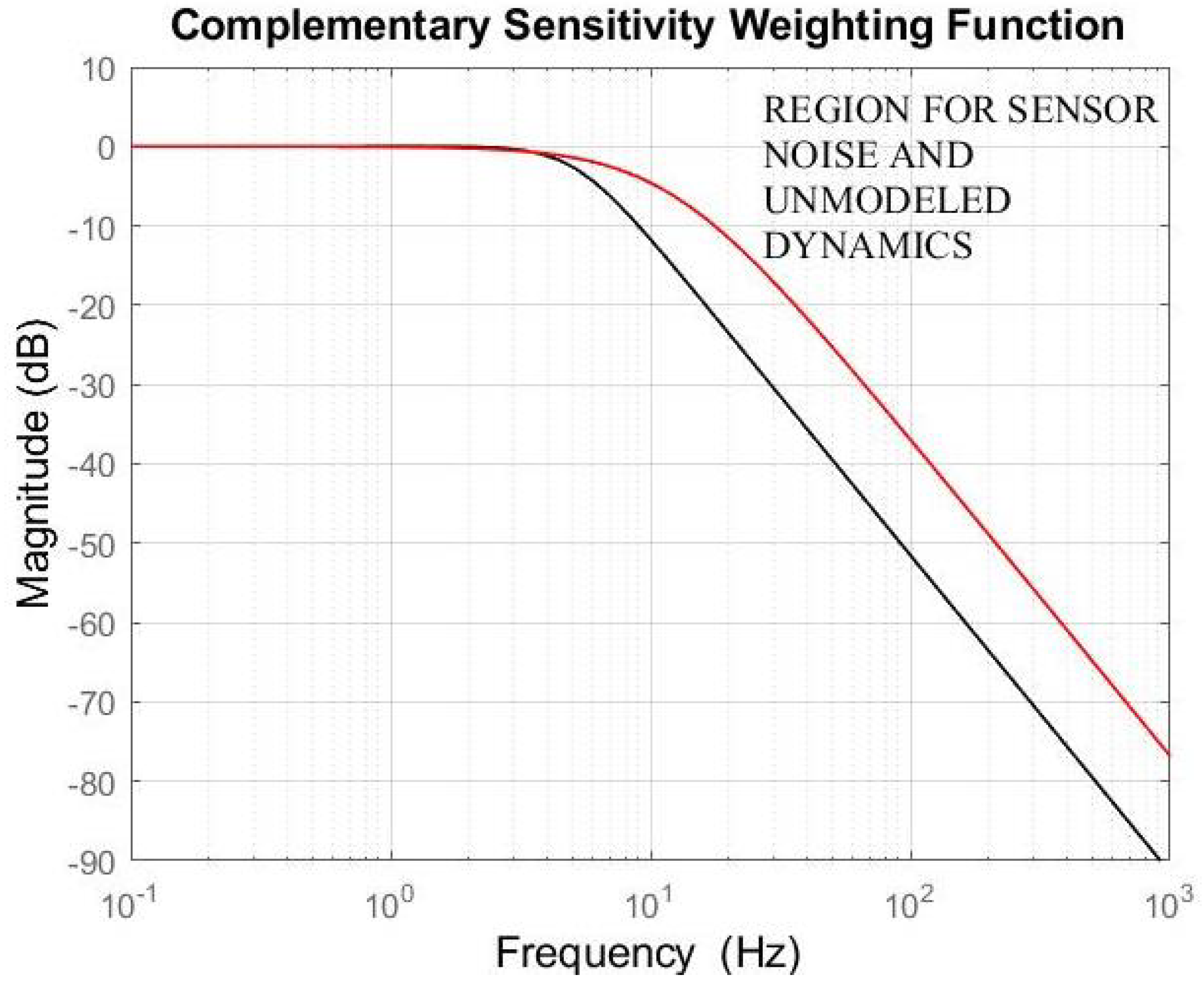
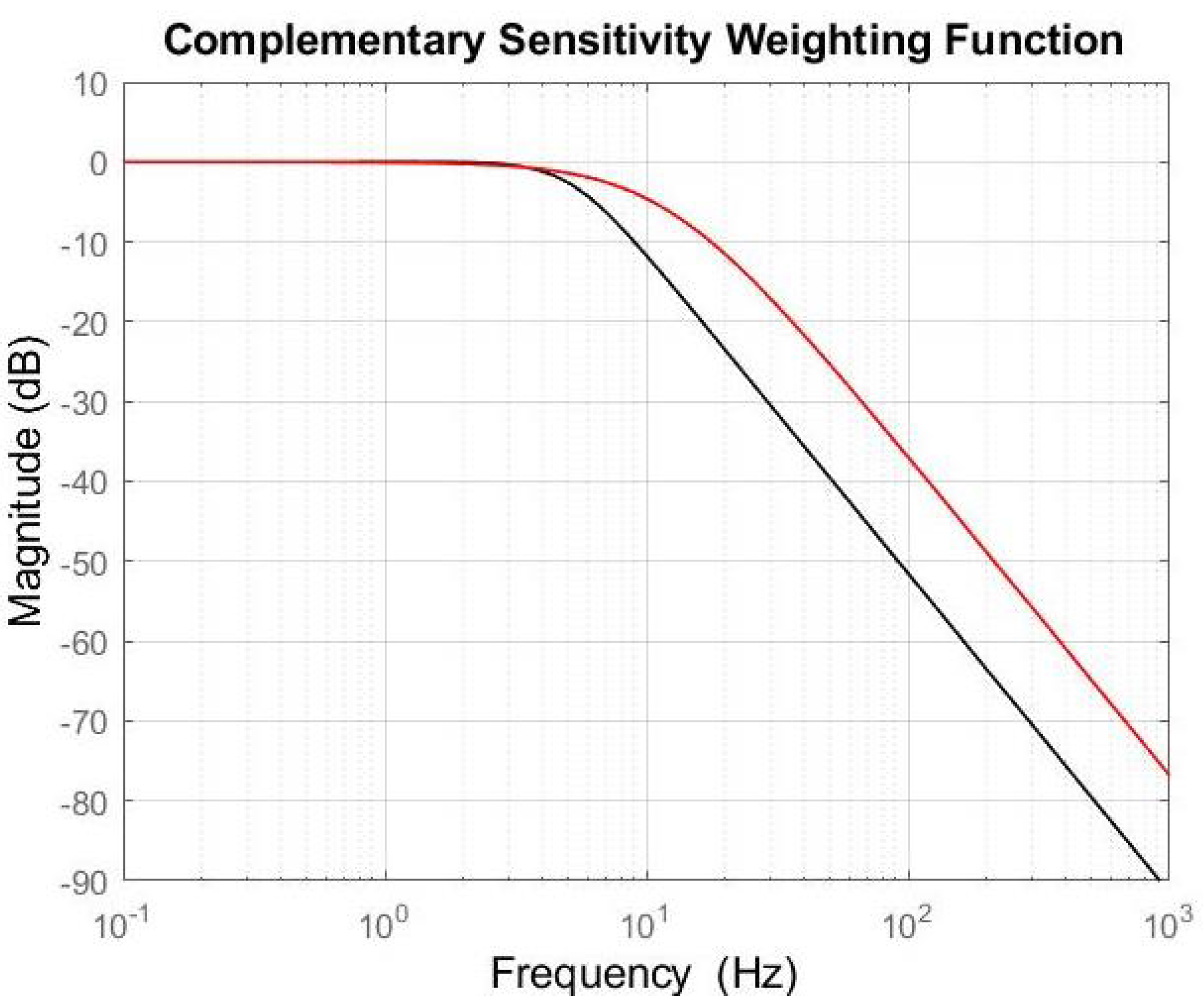
can be designed as a simple low-pass filter (as in Figure 5):
where is chosen again by trial and error.
The definition of the weighting functions represents the crucial aspect of the design. They reflect the system frequency requirements, but they also influence the system robustness and the quality of the time responses. Even if, in their original formulation, they are able to satisfy the robustness performances of the system, it is not guaranteed that a satisfying behavior is achieved in the time domain. Moreover, and cannot be used exactly as in (4) and (9), since they are not stable and proper functions: has a pole at the origin, while is an improper function. The introduction of two new supporting functions, and , allows fixing such an issue, defining them as:
and will replace and in the formulation of the generalized plant. In (10), is chosen as a low-frequency pole substituting the pole at the origin, which makes the function unstable; defines the order of the system: corresponds to the number of poles at the origin of the controller, and p corresponds to the number of poles at the origin of the plant.
The choice of the pole, as well as possible uncertainties in its actual location, do not represent a critical issue. The only requirement is that it has to be a low-frequency pole for the controlled robot. The quality of the dynamic model of an industrial manipulator included in its control architecture is usually more than sufficient to establish the entire frequency range well, by distinguishing low-, middle-, and high-frequency intervals. Moreover, it must be noted that the technique is based on the loop-shaping one. So, any tiny discrepancies do not involve significant changes in the system performances, and they can be possibly fixed at run-time if needed, for example, by modifying the controller crossover frequency.
In the next sections, we will prove that such a choice of and , and consequently of and , when applied to the control of an axis of a real industrial manipulator, may lead to good motor responses, but it can cause some link oscillations that cannot be accepted in the industrial context, where precision is the main task. We will then propose a different formulation, allowing significant improvements of the control performances.
3. Implementation to a Manipulator Axis
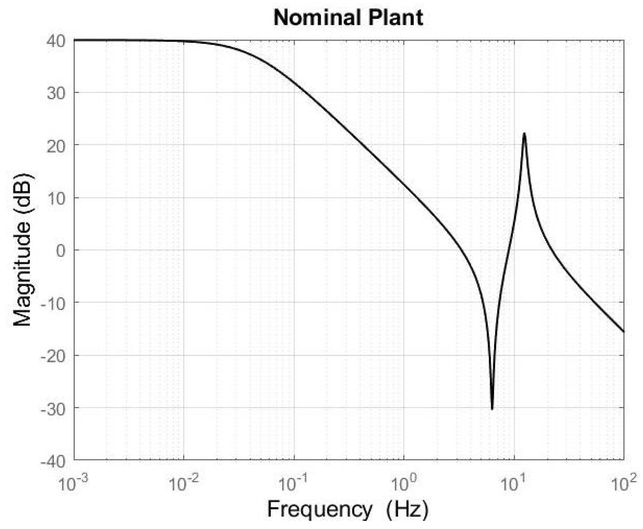
Let us consider for the nominal plant the following dynamic model of a base axis of a spot-welding Comau industrial manipulator, coherent with the general formulation given in (2), where all the numerical values are obtained expressing the robot physical parameters in SI units, and Nm/A:
The system is not very rigid: as it can be noticed from the Bode diagram of the transfer function module (Figure 6), its vibration mode is around 6 Hz. This makes the control implementation quite complex. Our purpose is to design and implement a control law able both to provide a precise axis response and to damp possible link vibrations. In order to make this possible, the control system has to work over the system modal frequency, e.g, at about 7 Hz.
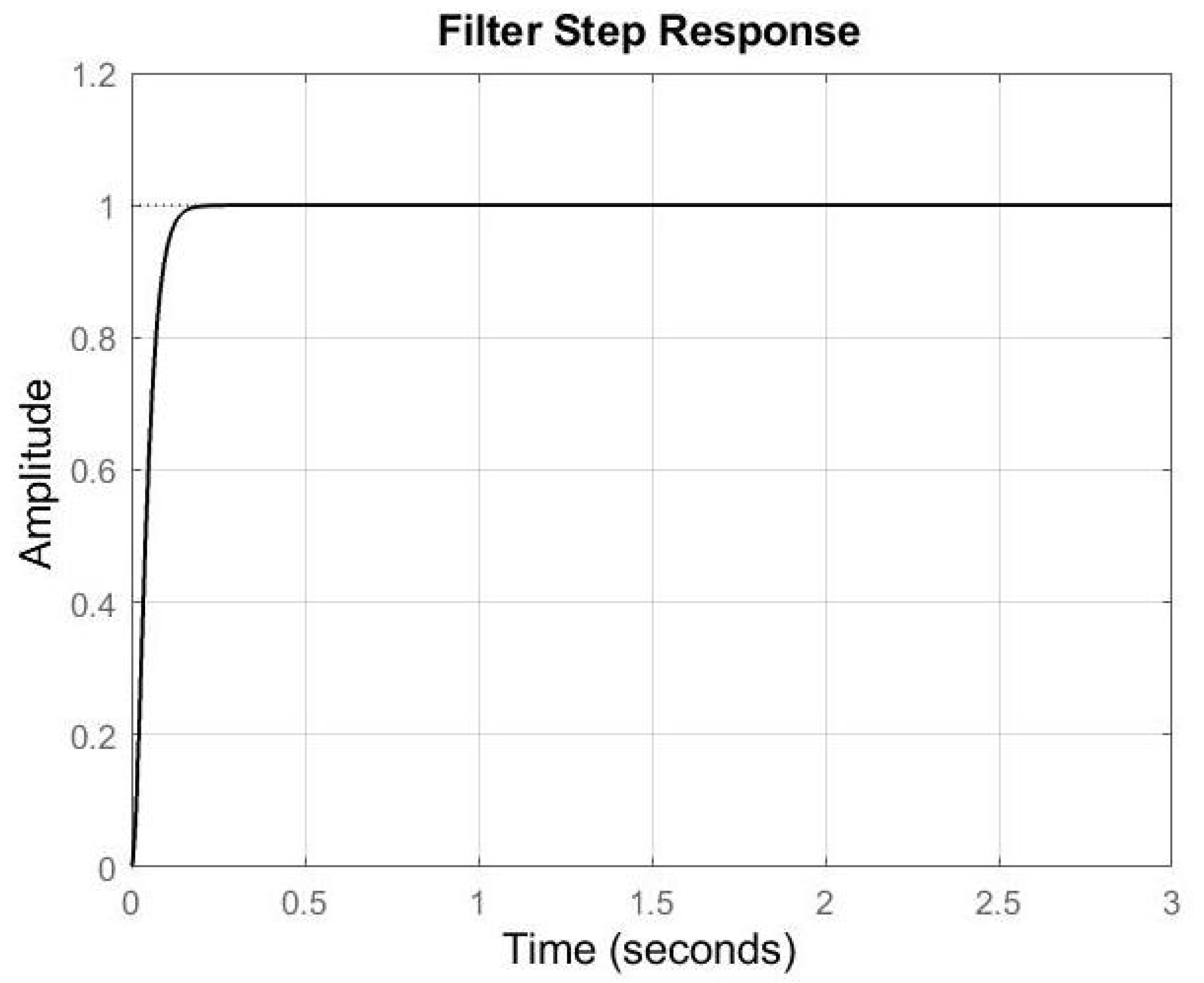
The time requirements to impose in the development of the controller are determined starting from the step response (reported in Figure 7) of a low pass filter satisfying the condition above, considered as the ideal desired behavior of the system.
The rise time and the settling time are evaluated from the step response plot as:
- = 0.112 s;
- = 0.134 s.
The last missing requirement regards the overshoot. Ideally, we would like to have a system with no overshoot. Since, in practice, this is hardly obtainable (and not always convenient), a maximum overshoot is considered as tolerable.
So, the general time specifications used in the control design are:
- = 0.112 s;
- = 0.134 s;
- = 0.05.
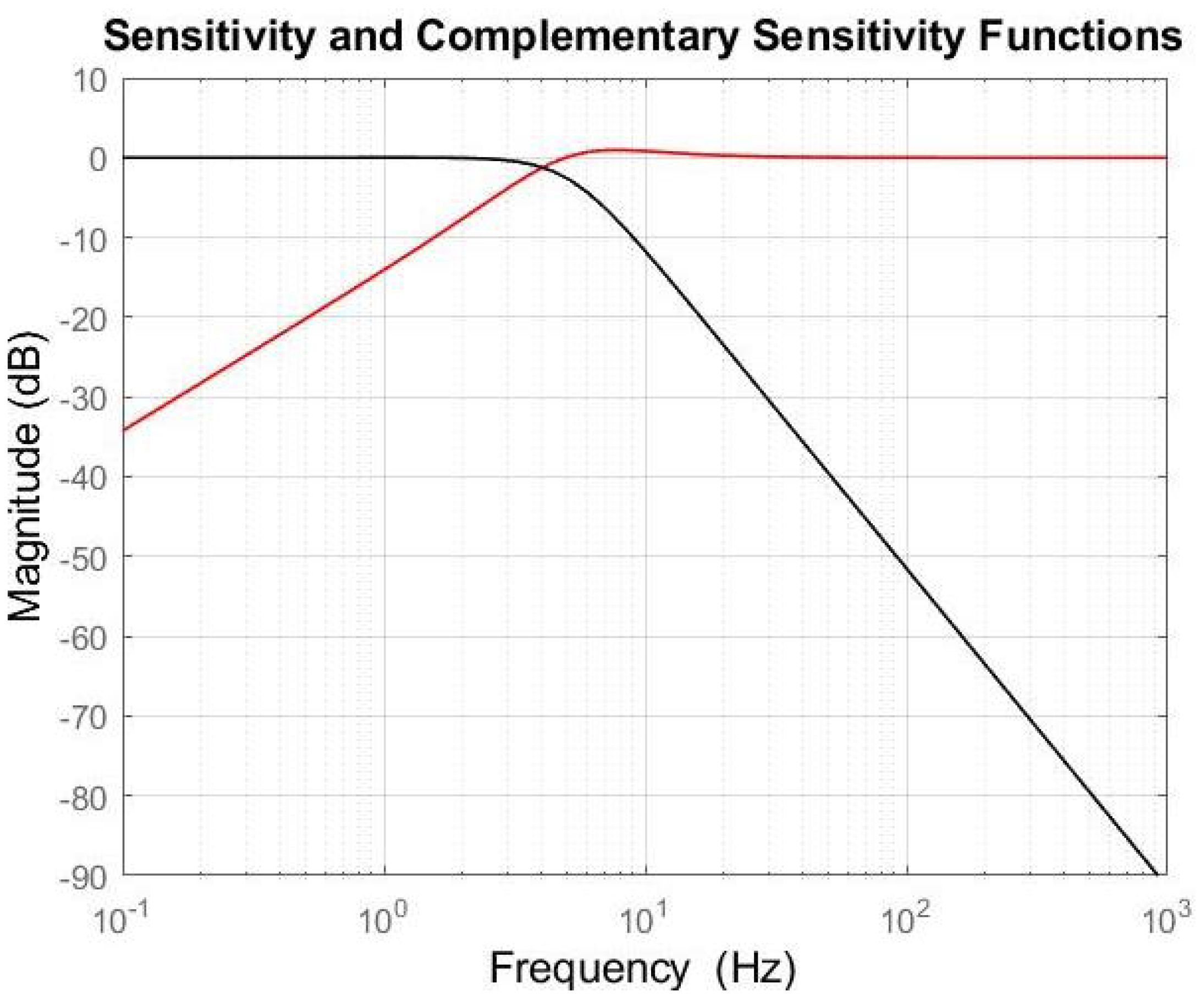
They are then translated into frequency domain requirements, leading to shapes of the sensitivity function and the complementary sensitivity function as reported in Figure 8.
According to the definition of the weighting functions (4) and (9), after some iterations, the nominal functions and can be shaped as in Figure 9 and Figure 10, respectively.
The controller transfer function is determined by solving the optimization problem through the “hinflmi” Matlab function, which implements the LMI-based approach [22].
By considering as state of the plant a vector including all the state variables corresponding to minimal realizations of , , and (which substitute and , as previously discussed), the best controller transfer function is obtained as:
[γ, Gc]= hinflmi(M, R, G, tol, opt).
The reader is recommended to refer to the Matlab help guide for command details.
The toolbox returns the controller in a system matrix form. Its subsequent conversion into the corresponding rational transfer function usually allows to apply some improvements. In fact, the function may include high or low frequency poles and zeros that can be removed to reduce the controller’s order, without causing any significant variation in the system time-step response. In addition, the solving procedure adopted by the toolbox does not include possible requirements about the presence of a pole at zero frequency in the controller. For example, by considering the velocity loop, it is useful to have a pole at zero in order to guarantee a null velocity error, while in the position loop, the s-pole derives from the position plant, where it is inserted in order to reach the physical and mathematical conversion from velocity to position.
Other changes that can be applied to the controller transfer function can regard its dc-gain, which can make the system slower or quicker.
By considering the actual control problem, the controller obtained by the LMI optimization is:
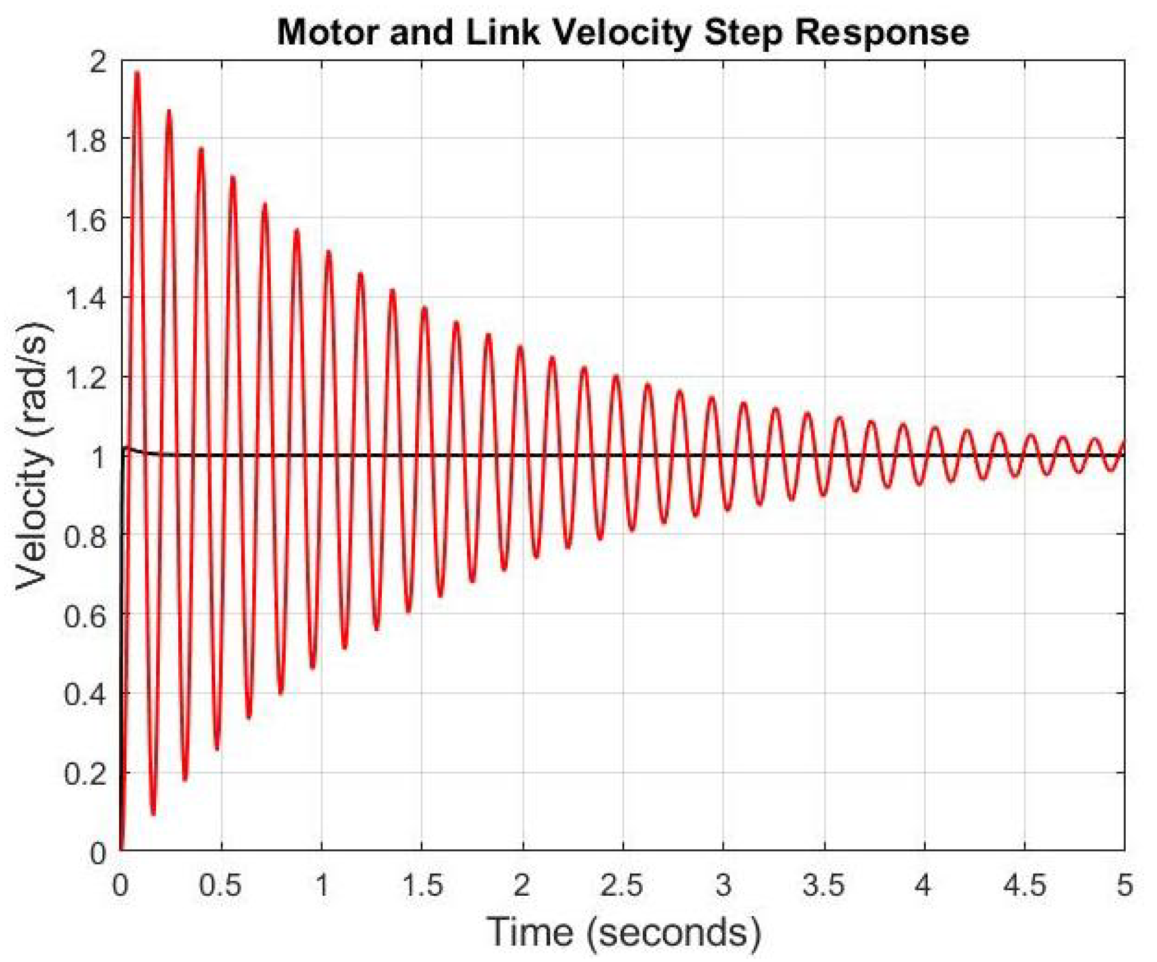
Figure 11 shows the motor and the link time responses obtained in simulation, by applying such a controller and evaluating the link behavior considering the following expression for the link model transfer function:
In the software implementation, the velocity controller is converted from continuous time to discrete time, guaranteeing the maintenance of the same phase margin, and then transformed into a series of second-order IIR filters, thus avoiding any possible problem related to high-order controllers. A similar procedure, which is quite common in the industrial context, will be followed for the implementation of the position controller, too, in the next section.
As it is evident from Figure 11, the simulation results are satisfying on the motor side, but they show an unacceptable behavior on the link side. The small overshoot in the motor response can be reduced or almost eliminated by the position control loop, not considered yet. On the contrary, the high vibration that characterizes the link behavior, and begins to damp only after 5 s, cannot be realistically eliminated by any control solution adopted for the position loop.
For the sake of completeness, and in order to evaluate the control robustness, a more realistic situation, in which some load is connected to the link, has been tested, augmenting the link inertia by about of its original value. As it is evident from Figure 12, the motor response still shows good performances, but the link vibrations are unacceptable anyway.
The robustness that theoretically and intrinsically characterizes the control approach is then confirmed, but unfortunately, the behavior of the part of system from which no direct measure is available, i.e., the link, is not satisfying.
Considering the obtained velocity results, it is necessary to modify the velocity controller before dealing with the position control loop.
4. The Plant Dynamics Cancellation Issue
At the basis of the theory, there is the resolution of the optimization problem (1), according to one of the possible, well-known ways [22]. The adopted “LMI approach” [22] satisfies the imposed requirements by inserting the inverse of the plant in the controller function definition. As a matter of fact, when the closed loop function is computed, the plant dynamics are canceled. This action does not guarantee satisfying results in a case like the considered one, where the transmission zeros are the only way to represent the system vibration modes and, consequently, to control the triggered vibrations. Their omission would make the system blind in front of the excitation of their frequencies. In case of a direct link control, this problem would not appear, since the link vibrations would be captured by a gyroscope sensor, and the application of the control through the standard LMI approach to solve the optimization problem would lead to good results. A possible solution to successfully design and implement the controller is developed in the next section.
5. A New Implementation Approach
The proposed modification is based on the idea of keeping the plant dynamics as partially visible from the control action. The elimination of the resonant zeros of the motor loop plant occurs in the standard implementation, when computing the closed-loop transfer function, because such zeros appear as poles of the controller transfer function. This derives from the choices made for the definition of the two weighting functions. As already explained, the weighting functions represent a mathematical way to describe the requirements that the system has to guarantee. The idea is then to let them also include the necessity to maintain the plant transmission zeros in the definition of the closed-loop function, in addition to the frequency domain requirements.
The proposed approach can be sketched as follows. Let us consider a plant transfer function expressed as:
where has the same structure of the model in (12), defining the relationship between the motor torque and the motor velocity.
The first step to perform is to choose the control specifications. Usually, in order to have a responsive system, it is preferable to close the control loop at a frequency higher than the plant vibration mode, defined by the plant resonant zeros. This means that if a vibration is registered at frequency, our purpose will be to have a control system working at frequency.
It is possible to understand that the frequency requirements are very important, and they have to be chosen carefully. In fact, they represent the starting point for the new definition of the and weighting functions.
In the standard implementation, developed in the previous sections, the sensitivity and the complementary sensitivity functions have been shaped starting from the value of the frequency of the imposed poles, derived from transient specifications, as:
The key point of the new implementation is the derivation of and in such a way that they can both directly summarize the frequency control requirements and realize weighting functions able to guarantee proper motor and link responses. In this sense, the standard expression of given in (16) is substituted by:
including the numerator of in (15). The additional polynomial at numerator has high-frequency roots, and it is added in order to make the function proper, while the denominator represents the translation in the s-domain of the control frequency requirements, as usual.
In particular, the roots of polynomial are the imposed dominant poles, usually chosen close to the nominal plant vibration mode (i.e., 5 Hz in the considered case), with a very high damping factor (0.99 has been set in our implementation). and are positive real numbers, defining two further stable poles, located at higher frequencies.
The sensitivity function is then determined from the complementary sensitivity function according to the following well-known relation:
The computation of starting from can result in a very low frequency zero that usually is approximated by Matlab with a zero in the origin, making the function not suitable to be used in the definition of the weighting function, which would not be BIBO stable, as well as the corresponding generalized plant thus obtained to be adopted in the solution of the optimization problem. If this is the case, the pole in in will be substituted by a low-frequency pole corresponding to the factor .
The new weighting functions are then determined as:
As already pointed out, the most important advantage of this new formulation of the weighting functions is the partial maintenance of the plant dynamics when closing the loop. In the standard procedure, the zeros of the nominal plant are introduced among the poles of the controller, thus causing their cancellation when multiplying the transfer functions of the controller and the plant. The approach builds the controller starting from a generalized plant, which is substantially a feedback system relating and the original plant . With the new formulation of the two weighting functions, the expression of includes the zeros of the plant among its poles. This choice leads to the presence of the zeros of the plant also among the zeros of the controller, resulting in their cancellation in the controller expression. When closing the loop, by multiplying and the dynamics associated to the zeros of the plant will be re-introduced. This way, the action of the controller will automatically counteract the effects of the vibration modes of the link and attenuate them as any disturbance acting on the system. In other words, since it is not possible to directly measure the link vibrations, because only sensors on the motor side are available, their influence on the controlled plant is kept alive to allow the controller to attenuate it, as a disturbance.
The control optimization problem is solved again by means of the LMI Matlab toolbox, using the new weighting functions (20) and (21). The application to the considered system, given in (12), and a subsequent simplification of the resulting controller, as suggested in Section 3 (i.e., eliminating the very high frequency poles and substituting a low-frequency pole in about 0.009 with a pole at zero), allows us to obtain the following controller expression (to be applied instead of (13)):
By following similar steps for the position control loop, the position controller for system (12) is achieved as:
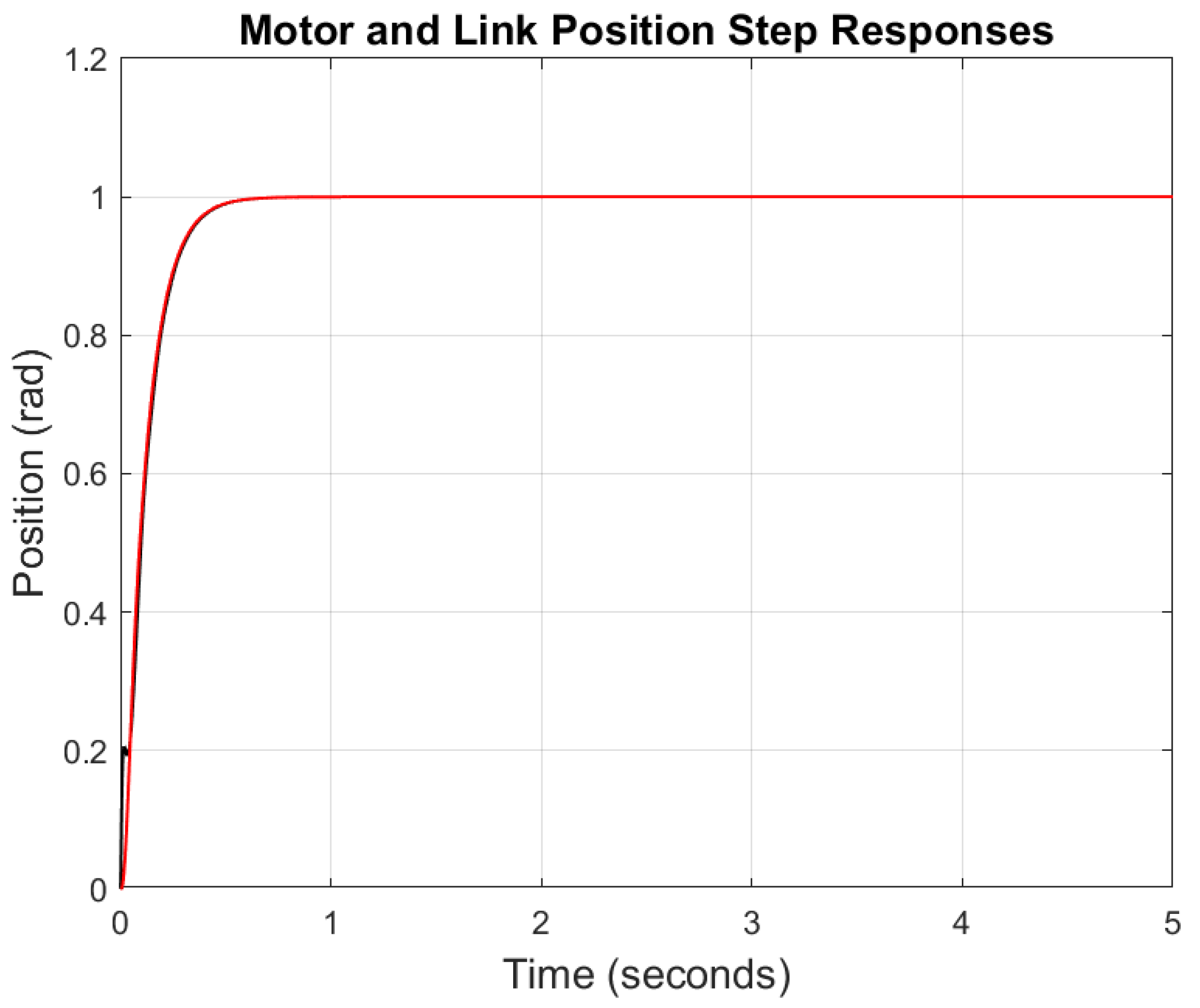
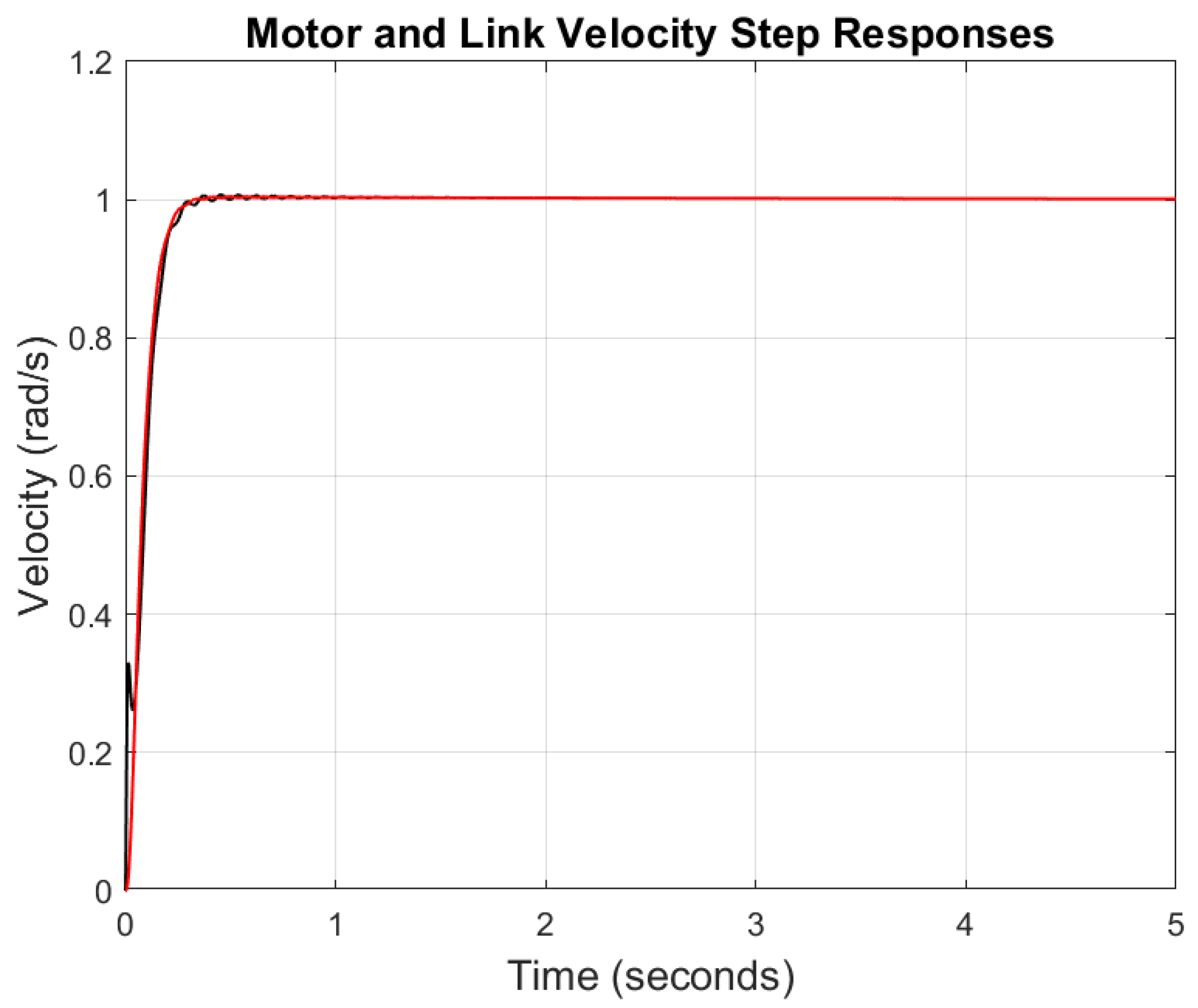
The application of controllers (22) and (23) provides much better results on both the motor and the link side, as it can be seen in Figure 13 and Figure 14, where the velocity and position time responses are reported, respectively. In particular, by comparing Figure 11 and Figure 13, showing the velocity step responses resulting by the application of the two control solutions, i.e., with the standard controller (13) and the modified one (22), respectively, it is possible to appreciate how, in the second case, the unacceptable oscillations of the link previously obtained have completely disappeared. Similar good results are achieved for the position, too, as shown in Figure 14.
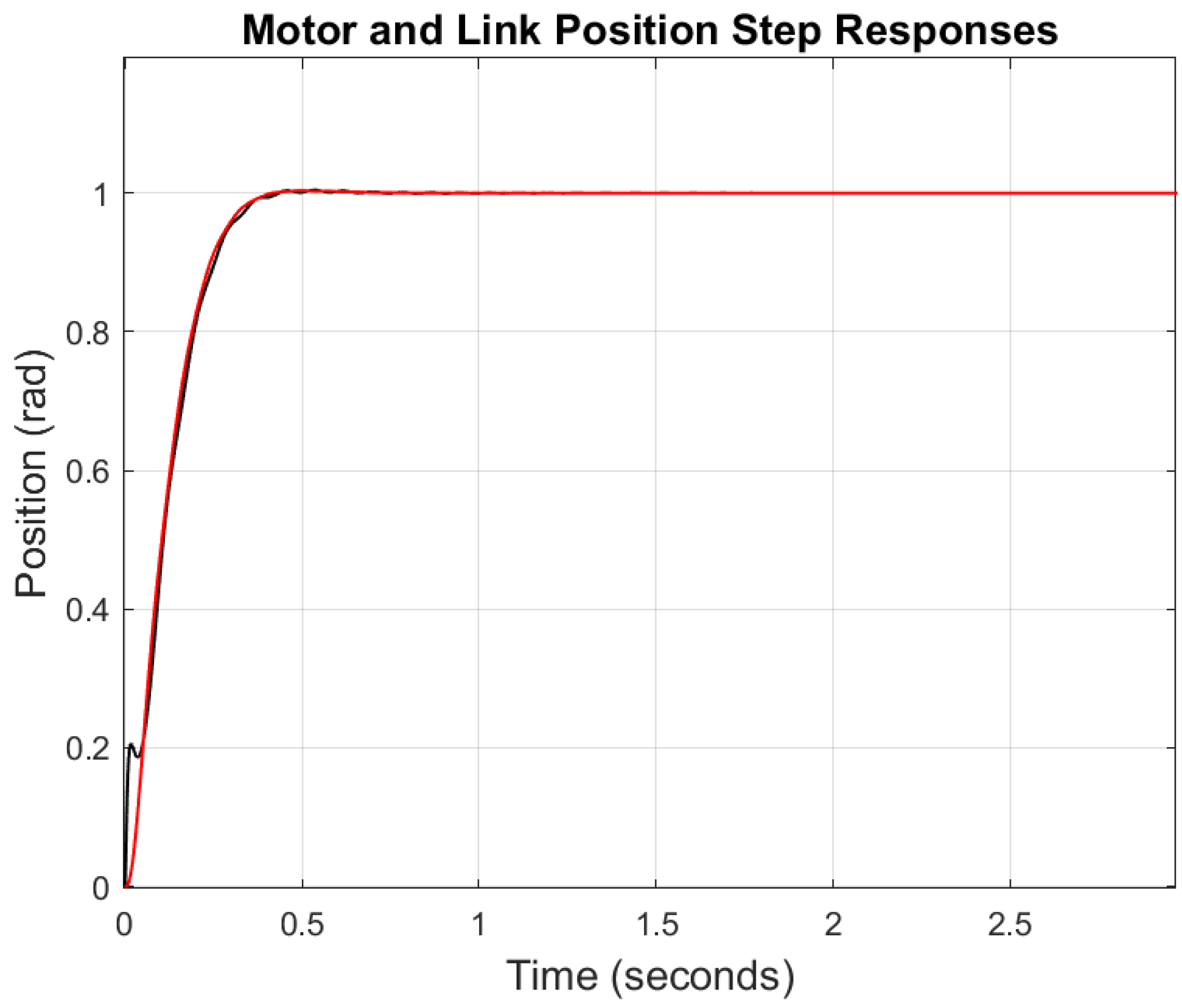
In order to prove the robustness of the control system to model uncertainties, the same variation in the link inertia considered in Section 3, corresponding to the increase of of its original value, has been applied. Figure 15 and Figure 16 show that, in spite of the important load variation introduced, satisfying velocity and position time responses are achieved on both the motor and the link side. The reader is invited to compare, in particular, the velocity time response reported in Figure 15 with the one previously obtained in Figure 12.
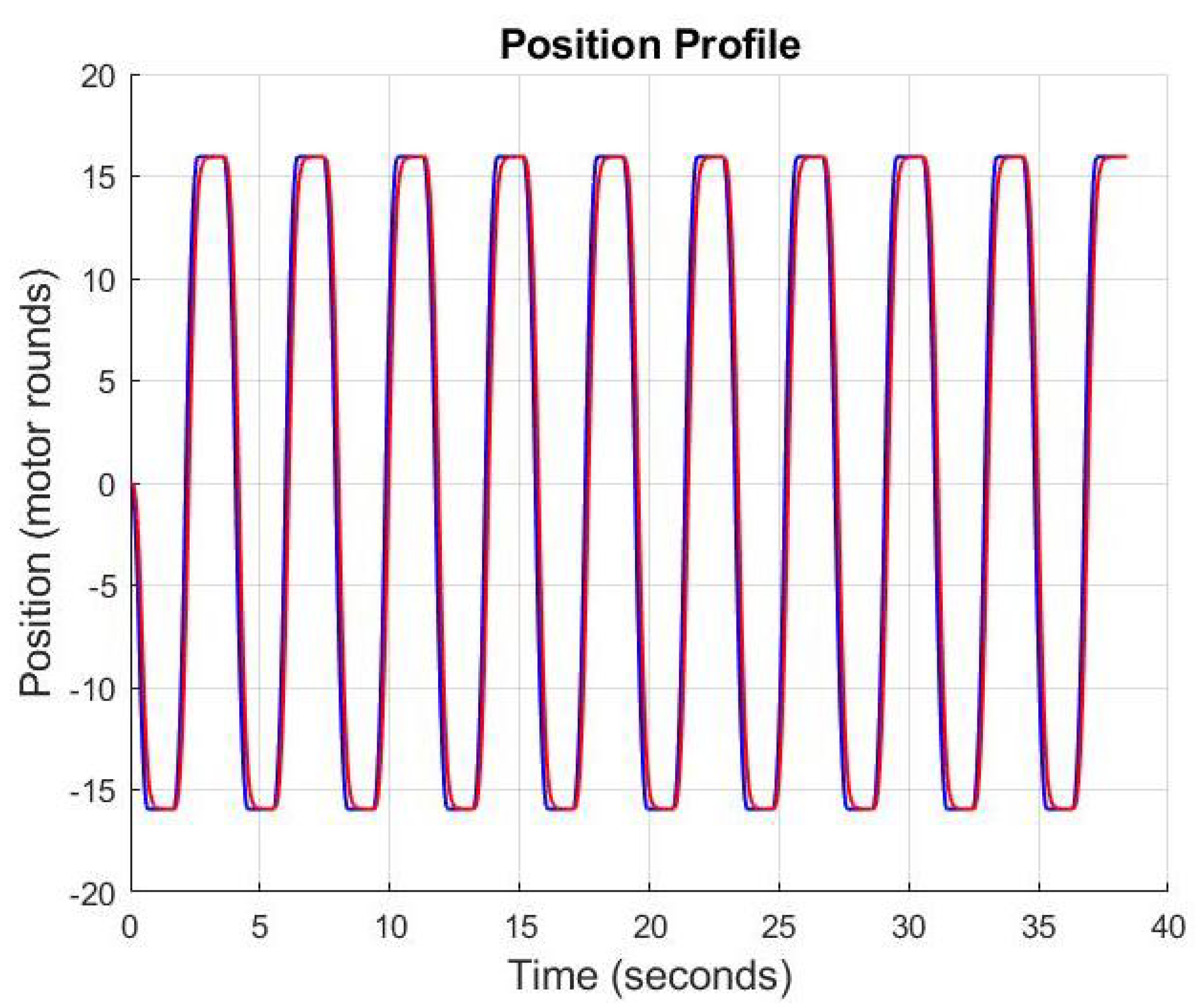
After having achieved satisfying velocity and position time step responses for both the motor and the link, a backward/forward reference trajectory has been applied to the axis, corresponding to the motion of the link between two desired positions. The simulation is performed in conditions similar to the real industrial operative ones, i.e., in presence of the disturbances on the single-axis system due to the load variations depending on the motion of the robot and to the interaction of the other axes.
The achieved simulation results, reported in Figure 17, confirm the validity of the proposed control solution.
It is worth noting that the delay between the reference and the measured position corresponds just to the one introduced by the control action.
6. Experimental Results
The validity of the proposed control solution has been finally tested on the real robot.
The test has been performed in the Grugliasco COMAU plant. The robot has been positioned in such a way to guarantee, for all the experiment duration, an inertia condition equals to 1547 Kgm, with its wrist axes in 0 0 orientation.
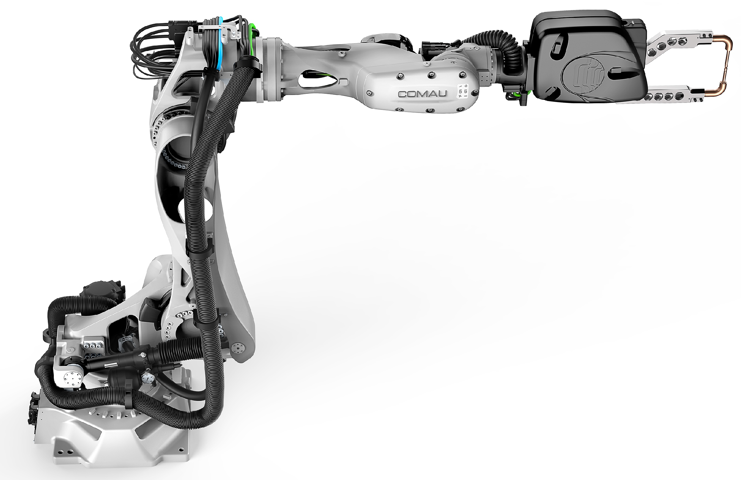
The considered axis of the robot, corresponding to model (12), has been moved in different positions by reproducing a spot-welding trajectory, which is among the most difficult tasks, since it is composed by isolated and short movements. For this reason, robots intended to perform them should be structurally very rigid. They have to stop with small settling time values and without triggering structure vibrations. From a mechanical point of view, the first axis of the kinematic chain should be characterized by a ratio between stiffness and inertial load as high as possible, which would result, from a control point of view, in models having resonant zeros at higher frequency. Figure 18 shows the new N220 Comau robot involved in spot operations.
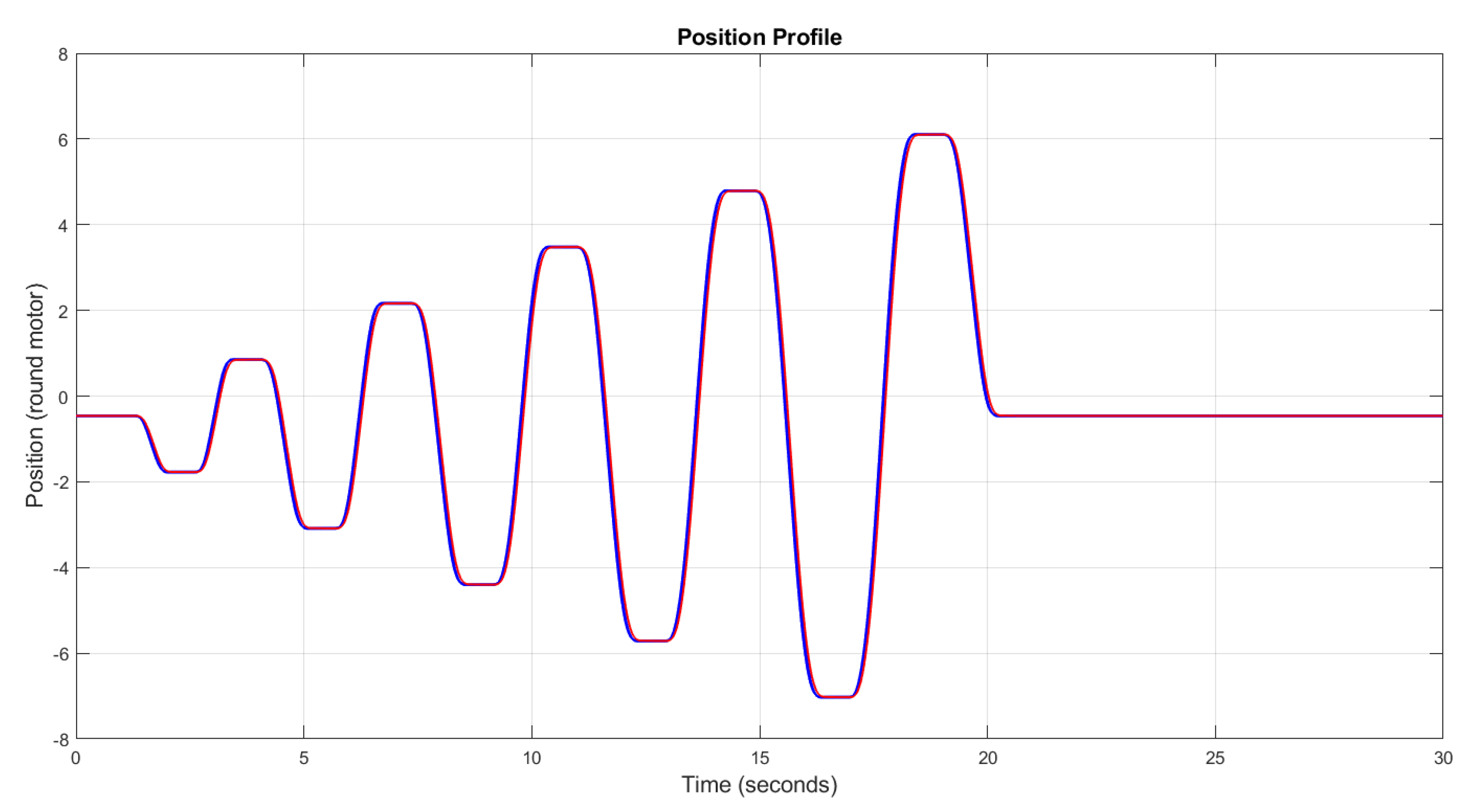
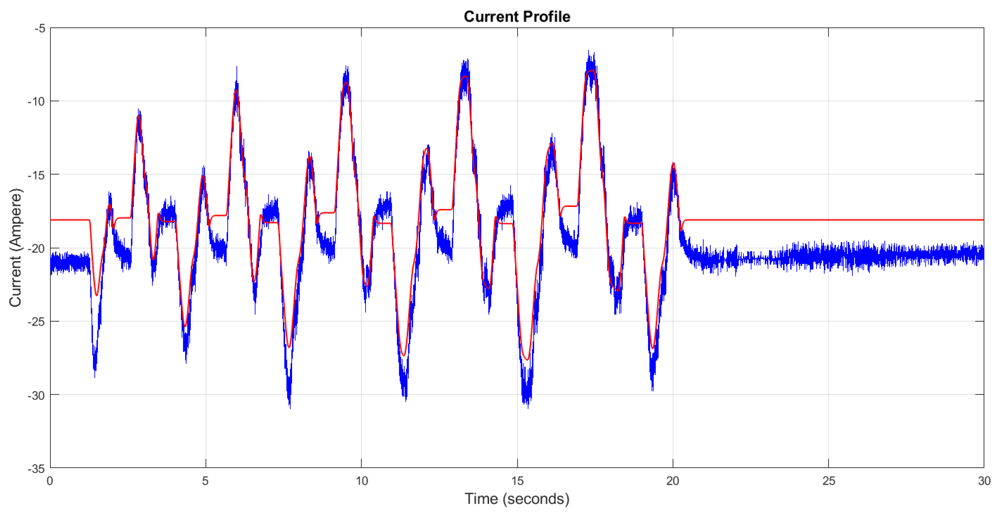
The results reported in Figure 19 confirm the simulation ones: the axis is able to track the entire reference path, without any significant vibration, as it can be evaluated also by the analysis of the motor current profile, reported in Figure 20.
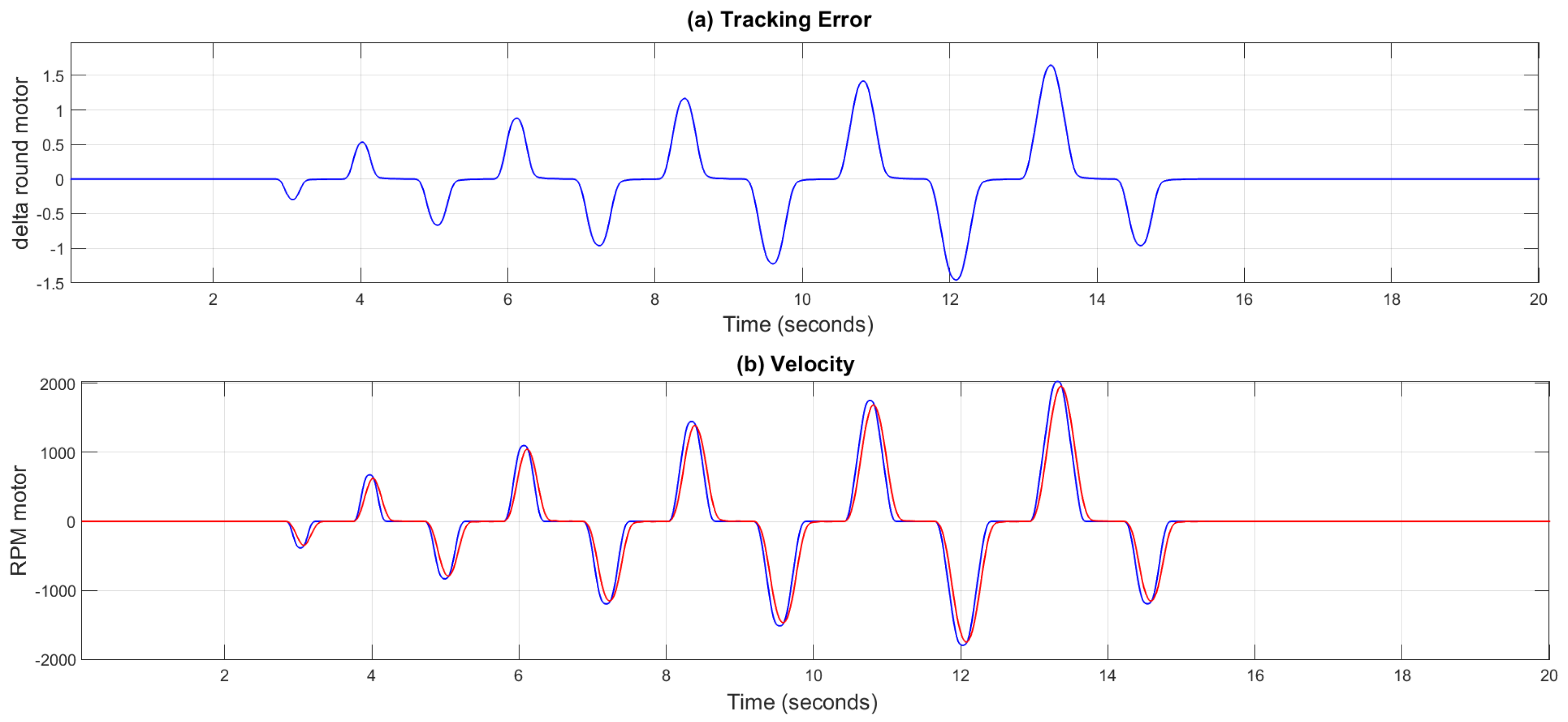
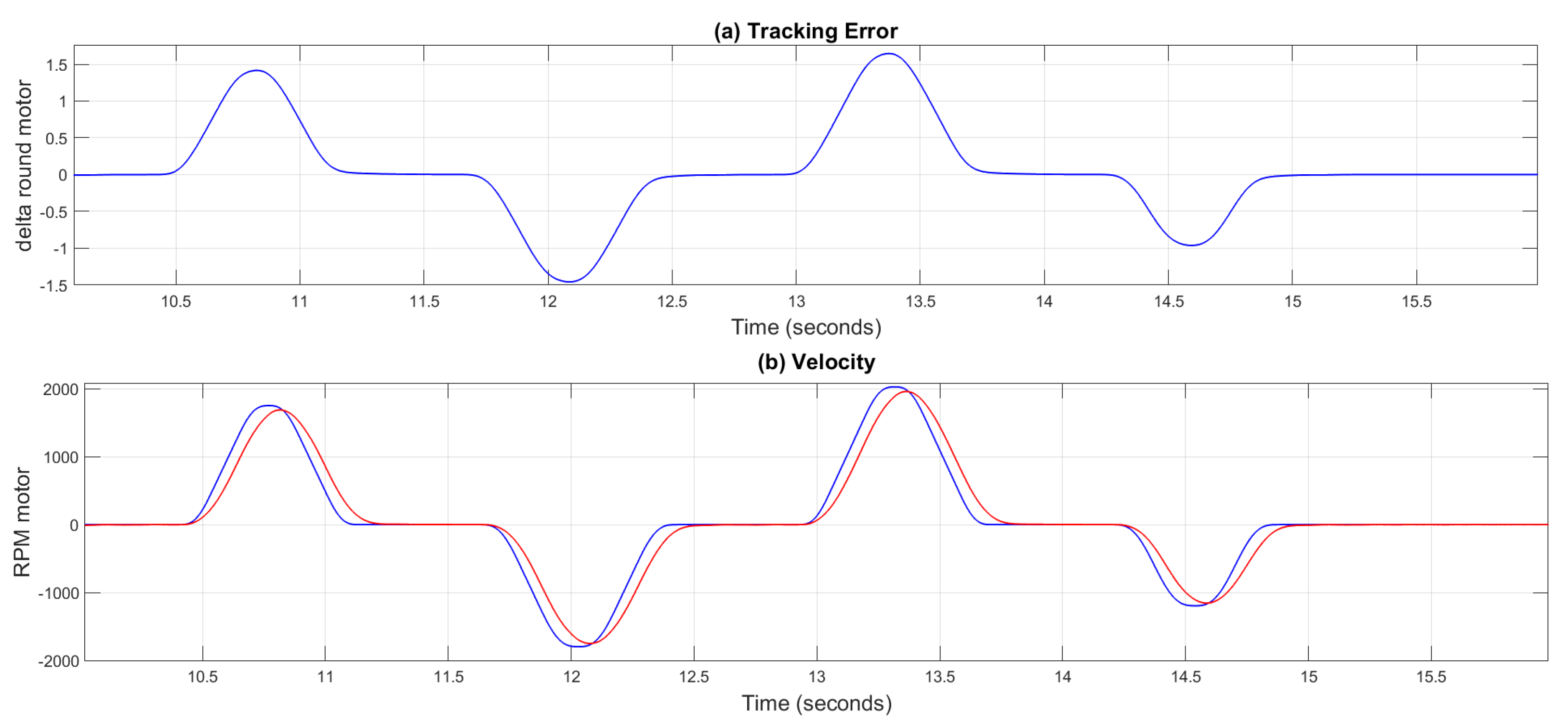
Relevant for our analysis is the tracking error, computed as the difference between the reference position and the measured one. Figure 21 compares the time-history of the tracking error with the velocity one for the entire robot motion, while Figure 22 provides a zoom in of the results in a shorter time interval. From such figures, it is possible to appreciate how the tracking error behavior reproduces the velocity one very well, thus indicating that the controller is behaving as expected.
The experimental results also show that the implemented controller is able to counteract possible disturbances deriving from the coupling with the other axes of the mechanical structure.
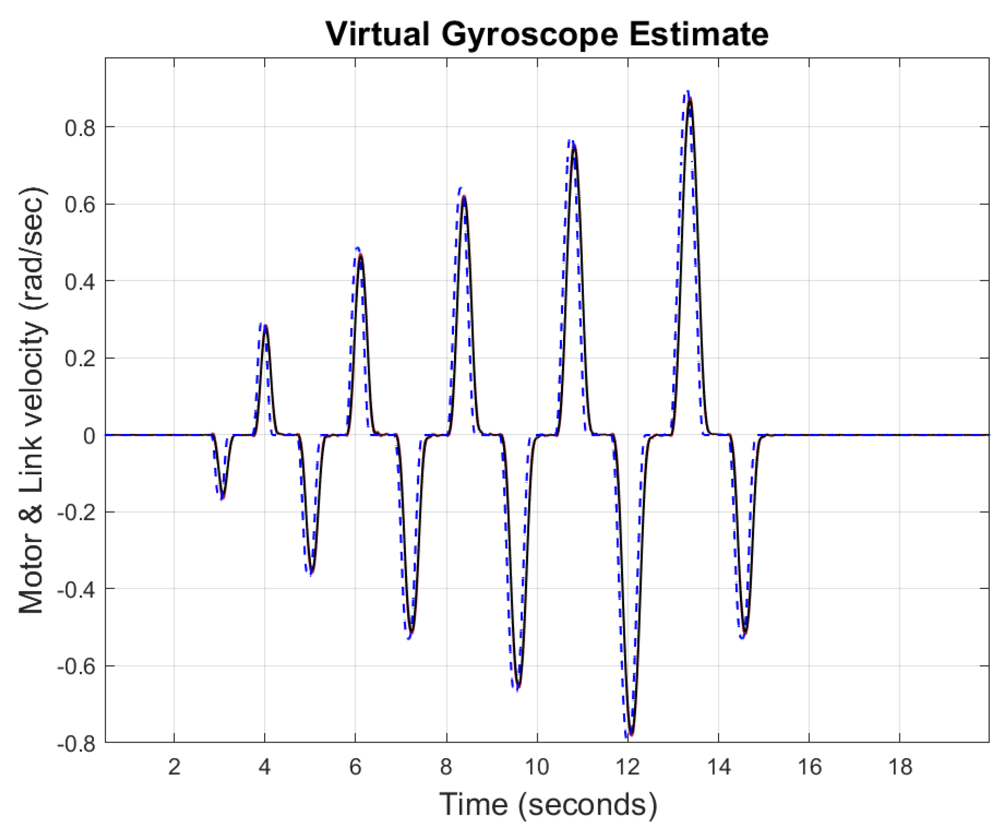
As previously discussed, the robot is not equipped with sensors on the link side. In order to evaluate the link response, it is possible to adopt some software solution able to estimate the link behavior. Figure 23 and Figure 24 show the estimate of the link behavior, obtained by a virtual gyroscope developed by COMAU as a strictly confidential instrument, used to evaluate in an approximate but reliable way the behavior of a link, avoiding the addition of sensors that are not part of the standard equipment.
The results shown in Figure 23 and Figure 24 confirm that the link is moving in a satisfying way. In particular, Figure 24 shows the absence of any relevant vibration of the link. The actual difference between the velocity profile values and the measured/estimated ones is mainly due to the characteristics of the applied point-to-point motion, which is a very closely spaced. In addition, it is worth remembering that the main objective of the applied nested loops control scheme is the position: a slightly imprecise velocity tracking is considered as absolutely acceptable in practice in point-to-point motions, when corresponding to a satisfying position tracking.
7. Conclusions and Future Works
In this paper, guidelines for the application of the approach to a motor-link control system have been determined for an industrial manipulator. In particular, the importance of a proper design of the weighting functions has been investigated. The partial maintenance of the system dynamics in the definition of the control action has allowed the proposed controller to provide robustness, high disturbance rejection, stability, and good performances on the link side, even if applied on the motor side, without any sensor located on the link. Both simulations and experimental results confirmed the validity of the proposed technique.
It must be noticed that the control system has been designed starting from a single operating condition, i.e., for a given vibration mode of the axis (of about 6 Hz) and the corresponding link inertia (of about 1547 Kgm). The problem is that, in order to perform its task, a robot does not remain trapped in a single position, but it moves by causing a change in the link inertia value. For this reason, future works will investigate the possibility of developing a Linear Parameter Varying (LPV) Controller, able to adapt to the various operative conditions and to guarantee an invariant time response over all the robot working area.
Author Contributions
Investigation, M.I., M.B., S.P. and V.P.; Methodology, M.I. and M.B.; Resources, S.P. and V.P.; Supervision, M.I., S.P. and V.P.; Validation, M.B.; Writing—Original draft, M.I. and M.B.; Writing—Review & editing, S.P. and V.P. All authors have read and agreed to the published version of the manuscript.
Funding
This research received no external funding.
Institutional Review Board Statement
Not applicable.
Data Availability Statement
Not applicable.
Conflicts of Interest
The authors declare no conflict of interest.
References
- Mesmer, P.; Neubauer, M.; Lechler, A.; Verl, A. Robust design of independent joint control of industrial robots with secondary encoders. Robot. Comput.-Integr. Manuf. 2022, 73, 102232. [Google Scholar] [CrossRef]
- Thomsen, D.K.; Søe-Knudsen, R.; Balling, O.; Zhang, X. Vibration control of industrial robot arms by multi-mode time-varying input shaping. Mech. Mach. Theory 2021, 155, 104072. [Google Scholar] [CrossRef]
- Kim, J.; Croft, E.A. Preshaping input trajectories of industrial robots for vibration suppression. Robot. Comput.-Integr. Manuf. 2018, 54, 35–44. [Google Scholar] [CrossRef]
- Shi, X.; Zhang, F.; Qu, X.; Liu, B. An online real-time path compensation system for industrial robots based on laser tracker. Int. J. Adv. Robot. Syst. 2016, 13, 172988141666336. [Google Scholar] [CrossRef]
- Tumari, M.M.; Saealal, M.S.; Ghazali, M.R.; Zawawi, M.A.; Shah, L.A. H∞ controller based on LMI region for flexible robot manipulator. Res. J. Appl. Sci. 2012, 7, 275–281. [Google Scholar] [CrossRef]
- Axelsson, P.; Helmersson, A.; Norrlöf, M. H∞ Controller Design Methods Applied to One Joint of a Flexible Industrial Manipulator. IFAC Proc. 2014, 47, 210–216. [Google Scholar] [CrossRef]
- Kim, M.J.; Choi, Y.; Chung, W.K. Bringing nonlinear H∞ optimality to robot controllers. IEEE Trans. Robot. 2015, 31, 682–698. [Google Scholar] [CrossRef]
- Ullah, M.I.; Ajwad, S.A.; Irfan, M.; Iqbal, J. MPC and H∞ based feedback control of non-linear robotic manipulator. In Proceedings of the 2016 International Conference on Frontiers of Information Technology (FIT), Islamabad, Pakistan, 19–21 December 2016. [Google Scholar]
- Rigatos, G.; Siano, P.; Raffo, G. A nonlinear H∞ control method for multi-DOF robotic manipulators. Nonlinear Dyn. 2017, 88, 329–348. [Google Scholar] [CrossRef]
- Hayat, R.; Leibold, M.; Buss, M. Robust-adaptive controller design for robot manipulators using the H∞ approach. IEEE Access 2018, 6, 51–626. [Google Scholar] [CrossRef]
- Liu, H.; Tian, X.; Wang, G.; Zhang, T. Finite-Time H∞ Control for High-Precision Tracking in Robotic Manipulators Using Backstepping Control. IEEE Trans. Ind. Electron. 2016, 63, 5501–5513. [Google Scholar] [CrossRef]
- Agbaraji, C.E.; Udeani, U.H.; Inyiama, H.C.; Okezie, C.C. Robust Control for a 3DOF Articulated Robotic Manipulator Joint Torque under Uncertainties. J. Eng. Res. Rep. 2020, 9, 1–13. [Google Scholar]
- Makarov, M.; Grossard, M.; Rodriguez-Ayerbe, P.; Dumur, D. Modeling and preview H∞ control design for motion control of elastic-joint robots with uncertainties. IEEE Trans. Ind. Electron. 2016, 63, 6429–6438. [Google Scholar] [CrossRef]
- Carreño, J.J.; Villamizar, R. Robust Control of Robot Manipulator based on QFT and H∞. Int. J. Electr. Eng. Comput. Sci. (EEACS) 2019, 1, 1–6. [Google Scholar] [CrossRef]
- Hwang, S.; Park, S.H.; Jin, M.; Kang, S.H. A robust control of robot manipulators for physical interaction: Stability analysis for the interaction with unknown environments. Intell. Serv. Robot. 2021, 14, 471–484. [Google Scholar] [CrossRef]
- Cruz, G.L.; Alazki, H.; Cortes-Vega, D.; Rullan-Lara, J.L. Application of Robust Discontinuous Control Algorithm for a 5-DOF Industrial Robotic Manipulator in real-time. J. Intell. Robot. Syst. 2021, 101, 75. [Google Scholar] [CrossRef]
- Lu, P.; Huang, W.; Xiao, J.; Zhiu, F.; Hu, W. Adaptive Proportional Integral Robust Control of an Uncertain Robotic Manipulator Based on Deep Deterministic Policy Gradient. Mathematics 2021, 9, 2055. [Google Scholar] [CrossRef]
- Rusnak, I. Family of the PID Controllers. In Introduction to PID Controllers; Panda, R.C., Ed.; IntechOpen: London, UK, 2012. [Google Scholar]
- Shang, Y. Resilient interval consensus in robust networks. Int. J. Robust Nonlinear Control 2020, 30, 7783–7790. [Google Scholar] [CrossRef]
- Kemin, Z.; Doyle, J.C. Essentials of Robust Control; Prentice Hall: Hoboken, NJ, USA, 1998. [Google Scholar]
- Bansal, A.; Sharma, V. Design and analysis of robust H∞ controller. Control Theory Inform. 2013, 3, 7–14. [Google Scholar]
- Gahinet, P.; Nemirovskii, A.; Laub, A.J.; Chilali, M. The LMI control toolbox. In Proceedings of the 1994 33rd IEEE Conference on Decision and Control, Lake Buena Vista, FL, USA, 14–16 December 1994; pp. 2038–2041. [Google Scholar]
Figure 1.
Feedback Control System.

Figure 2.
Closed-Loop architecture.

Figure 3.
General control software architecture of a COMAU industrial robot.

Figure 4.
Weighting Function—Black line: Sensitivity function; Red line: Weighting function.

Figure 5.
Weighting Function—Black line: Complementary Sensitivity function; Red line: Weighting function.
Figure 5.
Weighting Function—Black line: Complementary Sensitivity function; Red line: Weighting function.

Figure 6.
Nominal Plant.

Figure 7.
Low-pass filter step response, representing the ideal system behavior.

Figure 8.
(red line) and (black line).

Figure 9.
(black line) and (red line).

Figure 10.
(black line) and (red line).

Figure 11.
Motor and Link velocity time responses—Black line: Motor Response; Red line: Link Response.
Figure 11.
Motor and Link velocity time responses—Black line: Motor Response; Red line: Link Response.

Figure 12.
Motor and Link velocity time responses with variation in the link inertia—Black line: Motor Response; Red line: Link Response.
Figure 12.
Motor and Link velocity time responses with variation in the link inertia—Black line: Motor Response; Red line: Link Response.

Figure 13.
Velocity Motor and Link time responses—Black line: Motor; Dashed Red line: Link.

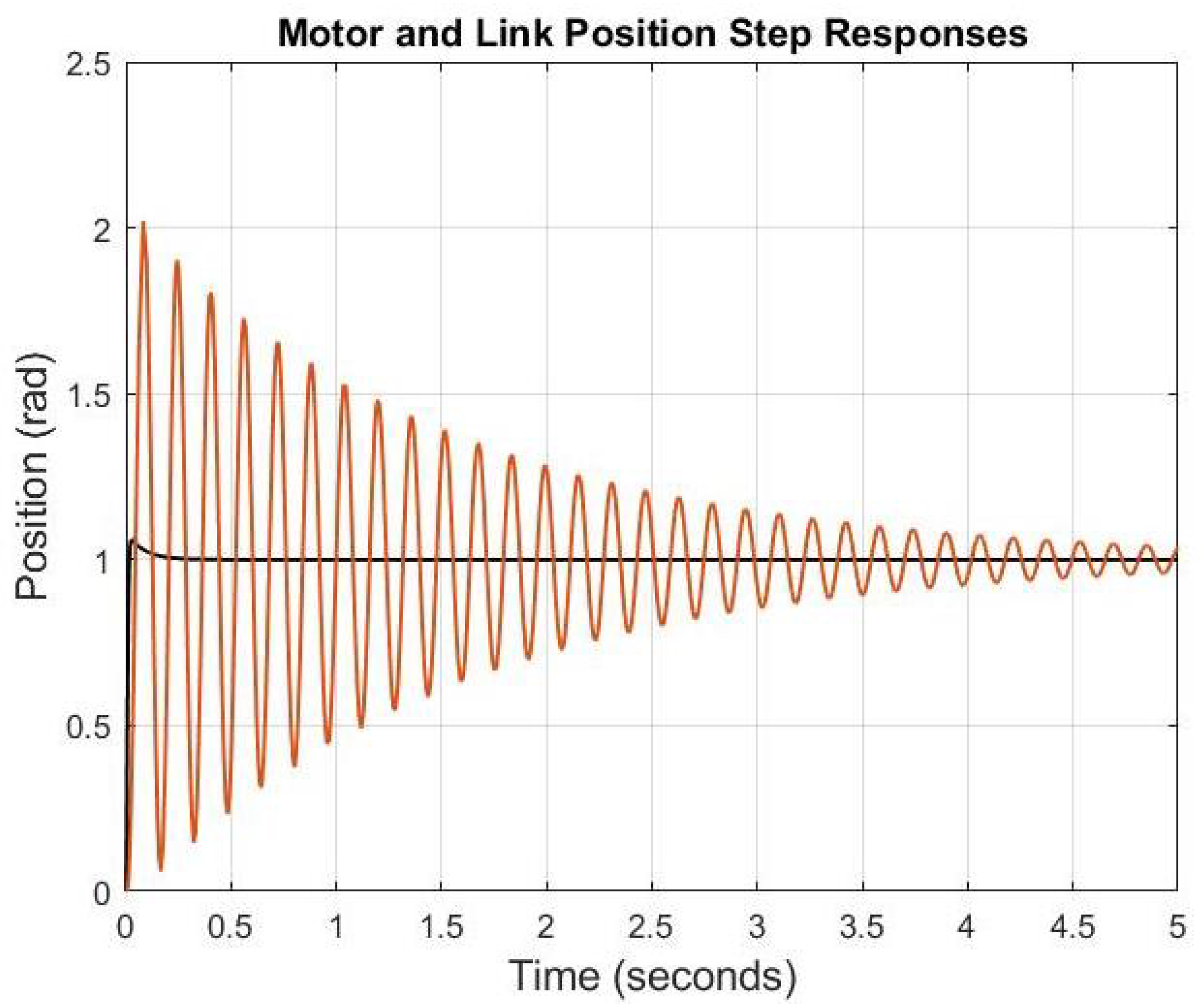
Figure 14.
Position Motor and Link time responses—Black line: Motor; Dashed Red line: Link.

Figure 15.
Motor and Link velocity time responses with variation in the link inertia—Black line: Motor Response; Red line: Link Response.
Figure 15.
Motor and Link velocity time responses with variation in the link inertia—Black line: Motor Response; Red line: Link Response.

Figure 16.
Motor and Link position time responses with variation in the link inertia—Black line: Motor Response; Red line: Link Response.
Figure 16.
Motor and Link position time responses with variation in the link inertia—Black line: Motor Response; Red line: Link Response.

Figure 17.
Simulated Real Position Profile (red line); Reference Position Profile (blue line).

Figure 18.
Comau robot N220.

Figure 19.
Experimental Position Profile (red line); Reference Position Profile (blue line).

Figure 20.
Real Current Profile (blue line) and Reference Current Profile (red line).

Figure 21.
(a) Tracking Error, (b) Velocity: reference profile (blue line), measured velocity (red line).
Figure 21.
(a) Tracking Error, (b) Velocity: reference profile (blue line), measured velocity (red line).

Figure 22.
(a) Tracking Error, (b) Velocity: reference profile (blue line), measured velocity (red line) in a shorter time interval.
Figure 22.
(a) Tracking Error, (b) Velocity: reference profile (blue line), measured velocity (red line) in a shorter time interval.

Figure 23.
Velocity reference (dashed blue line), motor velocity (black line), link estimated velocity (dark red line).
Figure 23.
Velocity reference (dashed blue line), motor velocity (black line), link estimated velocity (dark red line).

Figure 24.
Velocity reference (dashed blue line), motor velocity (black line), link estimated velocity (dark red line) for a single movement.
Figure 24.
Velocity reference (dashed blue line), motor velocity (black line), link estimated velocity (dark red line) for a single movement.

Publisher’s Note: MDPI stays neutral with regard to jurisdictional claims in published maps and institutional affiliations. |
© 2022 by the authors. Licensee MDPI, Basel, Switzerland. This article is an open access article distributed under the terms and conditions of the Creative Commons Attribution (CC BY) license (https://creativecommons.org/licenses/by/4.0/).
Share and Cite
MDPI and ACS Style
Indri, M.; Bellissimo, M.; Pesce, S.; Perna, V. A Robust H∞ Application for Motor-Link Control Systems of Industrial Manipulators. Appl. Sci. 2022, 12, 8890. https://doi.org/10.3390/app12178890
AMA Style
Indri M, Bellissimo M, Pesce S, Perna V. A Robust H∞ Application for Motor-Link Control Systems of Industrial Manipulators. Applied Sciences. 2022; 12(17):8890. https://doi.org/10.3390/app12178890
Chicago/Turabian StyleIndri, Marina, Martina Bellissimo, Stefano Pesce, and Valerio Perna. 2022. "A Robust H∞ Application for Motor-Link Control Systems of Industrial Manipulators" Applied Sciences 12, no. 17: 8890. https://doi.org/10.3390/app12178890
Note that from the first issue of 2016, this journal uses article numbers instead of page numbers. See further details here.