

Solar Irradiance Forecasting with Transformer Model

Department of Applied Informatics, Faculty of Natural Sciences, University of Ss. Cyril and Methodius, J. Herdu 2, 917 01 Trnava, Slovakia
*
Authors to whom correspondence should be addressed.
Appl. Sci. 2022, 12(17), 8852; https://doi.org/10.3390/app12178852
Submission received: 6 August 2022
/
Revised: 25 August 2022
/
Accepted: 28 August 2022
/
Published: 2 September 2022
(This article belongs to the Special Issue Intelligent Systems Applications to Multiple Domains Based on Innovative Signal and Image Processing)
Abstract
:Solar energy is one of the most popular sources of renewable energy today. It is therefore essential to be able to predict solar power generation and adapt energy needs to these predictions. This paper uses the Transformer deep neural network model, in which the attention mechanism is typically applied in NLP or vision problems. Here, it is extended by combining features based on their spatiotemporal properties in solar irradiance prediction. The results were predicted for arbitrary long-time horizons since the prediction is always 1 day ahead, which can be included at the end along the timestep axis of the input data and the first timestep representing the oldest timestep removed. A maximum worst-case mean absolute percentage error of 3.45% for the one-day-ahead prediction was obtained, which gave better results than the directly competing methods.
1. Introduction
Solar energy belongs to the primary sources of renewable energy, and its efficient use is a key factor in protecting the planet by reducing CO2 emissions. For future construction of solar farms as well as the placement of solar collectors on buildings, it is essential to know the ideal positions of these farms and collectors on the Earth’s surface [1]. Equally important for the regulation of energy networks is the ability to forecast solar power generation. For this purpose, the NASA POWER project focused on satellite measurements of solar radiation anywhere on Earth, which provides the data from 1984 to 2022 used in this article [2]. These data include both solar radiation and meteorological data for a given location. Meteorological conditions are correlated with the amount of sunlight [3].
The goal of this paper is to estimate the daily amount of solar radiation in various time horizons for a specified set of coordinates from regional data covering a square area of 2.5 × 2.5 degrees. This square dimension represents the local area from which the measurements are directly fed to the input of the neural network model used for prediction. By selecting a number of these smaller areas spread over a wider region, the model obtains a global view when predicting solar irradiance. The advantage of this combined solution is not only to obtain more inputs to the neural network, but the network learns to associate different combinations of local areas for more accurate solar irradiance prediction due to the attention mechanism built into the network. From the knowledge acquired during the learning process, this model can exclude irrelevant correlations between local areas’ data by suppressing information to higher layers and also learn to amplify information that is, in turn, essential to prediction. Point forecast data always represent the center of the area square.
A special type of deep neural network, the Transformer model [4], is used to predict how much solar energy will be produced in the near future. Transformer can find both temporal and spatial linkages in the input data and use them to predict the next-day solar photovoltaic power. The Python language and the TensorFlow [5] framework were used to implement the model (see Supplementary Materials).
In contrast to the research [6,7,8], the attention mechanism is implemented here using a Multi-head Attention layer rather than an LSTM or Bi-LSTM layer for temporal context features’ understanding. In the paper by Premalatha et al. [9], a classical ANN model with fully connected layers is described, which does not learn to contextualize features in long time series, as opposed to, e.g., the attention matrix. The papers [10,11,12] show the potential to break down the learning process into sunny and cloudy days. The studies [13,14] also show the advantage of using weather data as the input and describe the correlations between weather features and solar irradiance. The work [15] shows the possibility of segmenting clouds from an image and then expressing solar irradiance, thus opening the possibility of exploiting the very strong correlation between cloud cover and solar irradiance. The research [16] highlights several methods for processing satellite data to make very short-term forecasts of solar irradiance.
The Transformer deep neural network model has been specially adapted here to process all of the following intrinsically linked signals from different domains: solar irradiation, weather conditions, and position on Earth. These innovative space-time links between features, as well as point and regional data signal processing, enabled us to achieve a better one-day-ahead prediction. This was expressed by the maximum worst-case mean absolute percentage error of 3.45%, which is substantially smaller than that of directly competing methods.
2. Dataset and Methods
The following section is divided into two main parts. Firstly, a detailed description of the used dataset is provided, including solar irradiance signals, positions of the used regions on the Earth, where the signals were used, and their weather data, together with the necessary preprocessing. Secondly, the Transformer model for solar irradiance is specified, with its encoder and decoder parts, and spatial–temporal encoding. The limiting factor in forecasting solar irradiance is primarily weather, which strongly influences the performance, although the Transformer model used here is not directly focused on weather forecast. Though India is only ranked fifth in the publication Solar Power Capacity by Country [17], there have been many recent works predicting solar irradiance in this country [9,18,19,20]; hence, its dataset has been used in this paper to enable comparison with state-of-the-art prediction methods.
2.1. Dataset
For more accurate predictions of the amount of solar radiation, two types of data are fed to the input of the neural network. One source is regional data, and the other source is point-in-time data. Forecast is only for point data, while regional data are used as local areas around the point data.
To compare our results with state-of-the-art research, data from India were used. A total of 6 regions were selected with solar collectors located on buildings and 34 regions with large solar farms.
The entire process of downloading the dataset from NASA, as well as its preprocessing and subsequent export to CSV datasets, was ensured by a separate NASA POWER bot application. The bot application was implemented in the Julia language, which provided parallelism during download as well as data preprocessing. The CSV datasets, created in the previous step, were fed to the learning process in the Google Colab environment.
The dataset was split into training, validation, and testing sets. When the first 80% of the dataset ordered in time was used for training, the next 10% was used for model validation, and the last 10% created the test set. This particular time-ordered distribution of training, validation, and test sets resulted in tests that aimed to predict the future and, consequently, the learning pushed the model towards forecasting.
The biggest problem with the NASA POWER dataset is the lack of data to train the complicated Transformer model more accurately. After splitting the dataset into training, validation, and testing sets, only 11,136 examples are reserved for training, which makes training such a complicated model significantly more challenging. However, in the following years, by obtaining new data, this deficiency can be substantially compensated.
2.2. Region Pruning
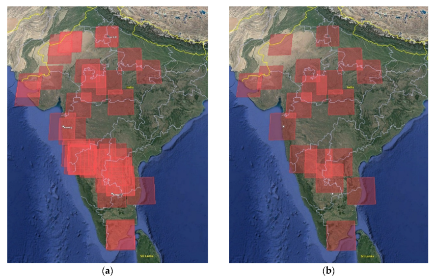
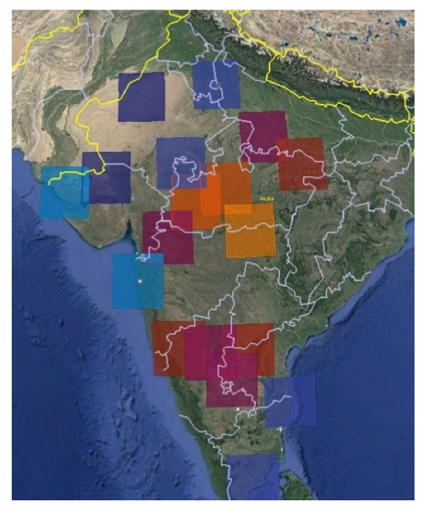
Since too many regions were selected, they had to be reduced. Many of the regions overlapped by a substantial area, and thus, following the results of the intersection over union algorithm [21], a number of these regions were excluded. If the regions overlapped by more than 25%, they had to go through the exclusion process. The removal was based on the comparison of the power and area of the solar collectors in the regions. If a region performed better, its “opponent” was excluded from the list of regions. If the power was not specified, the region with the smaller area of solar collectors was excluded. If neither power nor area was given, the decision was based on random choice, when each region had the same chance of exclusion. The exception was the regions marked as permanent, which excluded their non-permanent opponent automatically. If both regions were permanent, none were excluded. Figure 1 shows an example of such thinning of regions. It is evident that this thinning not only reduced the number of regions but also spread them over the surface of India to account for the largest possible global surface in global solar irradiance prediction. The total number of regions after thinning was 18.
2.3. Weather Characteristics
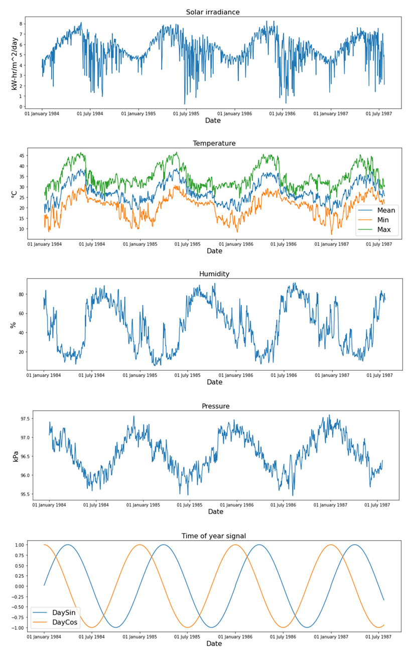
In addition to the data on the amount of solar radiation, the dataset also contained information about the weather. This information consisted of average, maximum, and minimum temperature; air humidity; atmospheric pressure; average, maximum, and minimum wind speed; and wind direction on a given day in the selected location. Figure 2 shows these measured variables over a period of 4 years, where it is possible to see the correlations between the temporal behavior of the individual variables during a day. It was therefore meaningful to include the weather as the input to the neural network. Another important feature for understanding the periodicity of weather and solar irradiance is the day of the year, which should not be directly fed into the input of the neural network and is transformed prior by Equations (1) and (2). Its preprocessing consists of converting the day of the year to sin and cos features, from which the network can more easily deduce the relationship between the period of the year and the repetition of patterns in weather and solar irradiance [22,23].
Information about wind direction and its speed also cannot be directly fed to the input of the neural network [22]. It is necessary to convert them to a wind vector [24] and then use the resulting vector as input features. The wind vector is defined by Equations (3) and (4), where ws is the wind speed in meters per second, and wd represents the direction of the wind in radians.
For the illustrative purposes of depicting the correlations between weather and the obtained solar irradiance, the years from 1984 to 1987 were used in Figure 2, which neatly captures the relationship between weather and solar irradiance. (The chosen 4-year range covers the initial period of training data; its selection from the available data does not have any deeper significance.) As can be seen from Figure 2, humidity is directly related to the amount of obtainable solar irradiance in such a way that, as humidity increases, cloud cover increases and thus shadows the sun’s rays. Therefore, it is also possible to derive the amount of the produced solar irradiance from the humidity. The orange curve in the time-of-year signal represents the DayCos, and the blue curve represents the DaySin as defined by Equations (1) and (2).
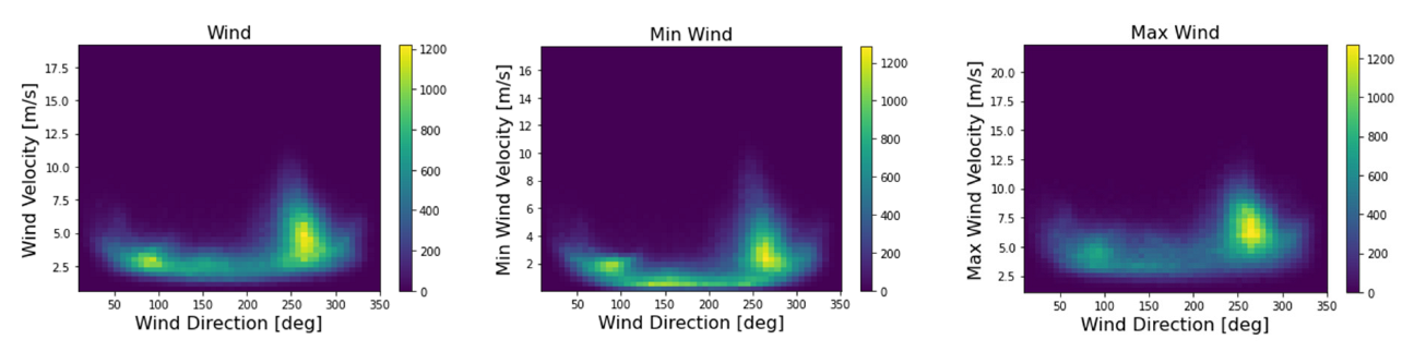
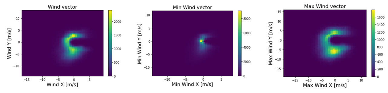
Figure 3 shows the relationship of wind speed to its direction, using a heatmap of the frequency of wind occurrence with a given speed at a certain angle. The graph shows that fast southwesterly winds are the most frequent; they also bring monsoons with them. Figure 4, on the other hand, shows the frequency of the occurrence of wind in the wind vector. As the figures show, the wind direction does not describe the whole circle, and thus, there are no winds blowing directly from the north.
2.4. Transformer Model for Solar Irradiance
The Transformer model is a neural network architecture used typically for natural language translation. Its basic element is the attention mechanism, which links related features in sequential data. Transformer is composed of basic parts, which are self-attention blocks and position-wise fully connected feed-forward network blocks. Self-attention blocks are formed by a normalization layer, a Multi-head Attention layer, a dropout layer, and finally a residual connection. Position-wise fully connected feed-forward network blocks are composed of a normalization layer, a pair of fully connected (dense) layers, a dropout layer, and finish with a residual connection. By stacking these basic blocks, two main parts of the model are created, the encoder and decoder. Self-attention block maps query and key-value inputs to one output from this block. The output is expressed as a weighted sum of the input value, where the weight is formed by the query input function with the corresponding key input, according to Equation (5). To improve the accuracy of the model, a combination of several attention matrices into one output was used according to Equation (6). The principle of the position-wise fully connected feed-forward network block is expressed by Equation (7) [4].
Here, the matrix Q represents the query input, the matrix K represents the key input, and the matrix V represents the value input to the attention block. The value dk expresses the size of the key input. Matrices represent trained model parameters for the projection of features [4].
The GeLU (Gaussian Error Linear Unit) in Equation (7) represents nonlinearity in the model [25], and matrices W and b represent weights and bias.
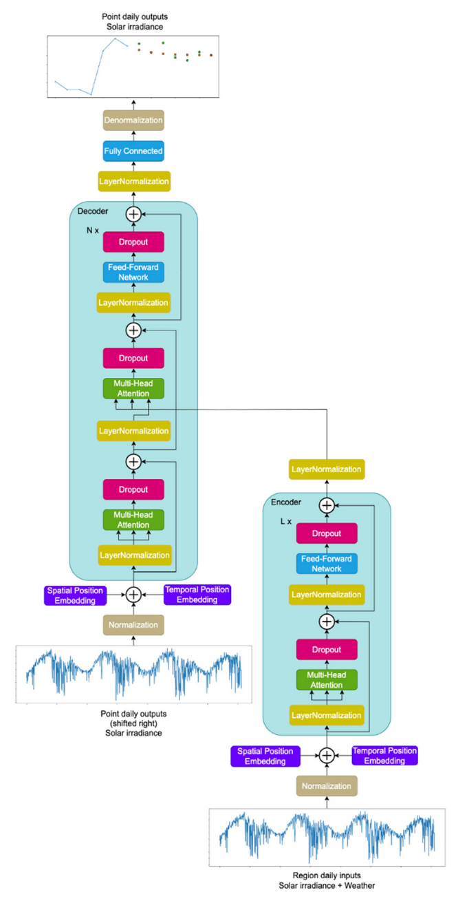
In the model used in this work (see Figure 5), unlike the original Transformer model [4], there are normalization layers before each block, and each block is terminated only by a residual connection, as is the case with the Vision Transformer, which, similarly to the problem of solar irradiance prediction, works on the input of the model with a real signal [25]. The truncated normal method with a standard deviation of 0.02 (as in the case of BEIT [26]) is used to initialize the training parameters of the model. The first input layer consists of a normalization layer adapted to training data, the task of which is to transform various measured physical variables with different ranges of values into variables with zero mean and unit standard deviation. The output from the model consists of a fully connected (dense) layer with the linear activation function that is followed by the denormalization layer, which helps to maintain a zero mean and one standard deviation of targets. The denormalization layer works in the same manner as the normalization layer but in the inverse.
The normalization layers and the denormalization layer are adapted to training examples only, and this is done before the training process. Their memorized values of means and standard deviations are also applied to both the validation and test datasets. The advantage of the last layer being linear is that the gradients are unaffected by the activation function of the neurons during the backpropagation since the first derivative of the linear function equals one. A learning rate cosine scheduler was also used for training, which optimizes the learning process [27] and allows the model only to warm up in the first steps of the learning process while the gradients are too high.
In the later steps of the cosine scheduler, the learning rate reaches a maximum from which it then only decreases until the end of the learning process, due to fine-tuning of the error of the model.
The input to the model is regional daily data, which contains a combination of past solar irradiance and past weather. Moreover, the model is fed with point solar irradiance data, which are shifted in a sequence during the prediction process of data points, in the sense that the oldest measurement is removed, and the last predicted measurement is lined up at the end of the data timeline.
2.5. Encoder
The encoder part of the model is used to convert the solar irradiance, weather, and day of the year into the latent space position. The goal of the encoder block is to look for mutual space–time bonds in the historical input data and convert them to latent space, which is the input to the next part of the model. Latent space is expressed for each timestep and location independently, as shown in Figure 6.
2.6. Decoder
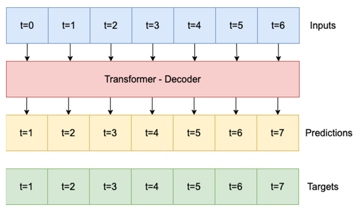
In the present case, the decoder block of the model works as a simulator of the future, which, by combining the historical point data, day of year, and latent space from the encoder, predicts solar irradiance 1 day ahead. This predicted day value can be brought back to the input of the model by connecting it to the original data shifted by one day to the right to obtain the next day. Figure 7 shows how the Transformer model predicts the next day. At every timestep, the decoder tries to estimate the next timestep. Future predictions are independently expressed for all of the Indian locations used.
2.7. Positional Encoding
Positional encoding is an essential part of every Transformer model, as this kind of neural network does not “recognize” the sequential order of the data, and the order within the data sequence could be mixed up. Therefore, it is necessary to add this kind of information to the input features at the beginning of the encoder and decoder parts of the model [4].
2.7.1. Temporal Information
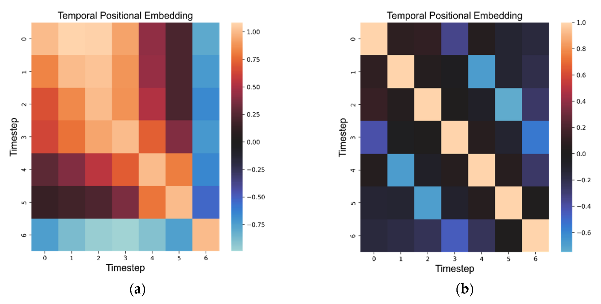
The temporal order of features at the input of the network is identified through 1D trained positions expressed by a vector added to the input of the model. This time information is essential to correctly understand the order of the timesteps and prevents the Transformer from mixing them up. As shown in Figure 8, the trained Transformer model clustered 1 day in the vicinity with the most similar properties. The days that are far apart in time have mostly a negative value of similarity in positional encoding of the decoder block. The encoder finds the strongest similarity in several days “around”.
2.7.2. Spatial Information
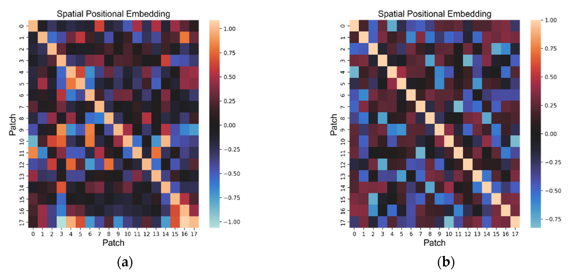
Like the sequence of timesteps, for the identification of the location of the measured region, the Transformer model also needs additional information expressing the unique 1D code of the given location. These identification codes are also expressed by a vector that is added to the input features. The network trains these identifiers by itself; thus, it can mark sites with similar meanings with a similar vector and, conversely, mark sites with no direct correlation with significantly different vector values. From Figure 9, it is possible to see the related regions, which, in most cases, overlap on the map of India. From this, it can be concluded that the trained Transformer model “understood” the spatial similarities and grouped them together according to their importance in predicting future solar irradiance. For a better explanation, Figure 10 shows similarity between the 0th patch and other patches on the world map. Here, it can be seen that the strongest similarity is in the neighboring regions, which have a reddish color corresponding to positive similarity.
2.8. Loss Function
The log-cosh function (see Equation (8)) was used as an error function in solving this type of regression problem. Its advantage over the typically used L2 loss function is its robustness against noise and outliers in the training data. With L2, it would be easier to become stuck in a local minimum. In comparison with another popular error function L1, which is robust to noise in the data, the log-cosh error function is smooth, which is better for the smoothness of the training process [28]. The log-cosh error function has proven to be a robust error function for the task of solar irradiance prediction.
2.9. Metrics
For estimation of the quality of the predicted solar irradiance, several metrics are typically used, such as mean squared error, root mean squared error, mean absolute error, mean absolute percentage error, and R squared. The emphasis should be put on the last predicted timestep, which represents the future solar irradiance, one day ahead. This practice is effective for selecting a model that best predicts the future. Mean absolute error expresses the error of solar irradiance directly in kWh/m2/day. During metrics calculation, timesteps before the last (future) timestep are not included, but, during training, all timesteps are used to calculate the gradients and provide important information to the model.
2.10. Simulation Phase
A trained model can be used to predict different time horizons, which is an advantage of this solution. The output of the model consists of the solar irradiance of the next day and can thus be fed repeatedly to the input of the model, making it possible to predict 2, 3, 4, 5, etc. days ahead. The problem is that the model input consists of day-of-year features, DaySin, and DayCos, in addition to solar irradiance. Thus, it is necessary to transform these features from the last timestep in the window to day of year, according to Equation (9). Then, add 1 day to this day and convert it back to the DaySin and DayCos features, according to Equations (10) and (11). The newly created DaySin and DayCos are merged with the predicted solar irradiance for the next day. The vector thus created can be fed to the model input. It does not make sense to train the model to predict DaySin and DayCos since it is designed to be fully focused on predicting only solar irradiance.
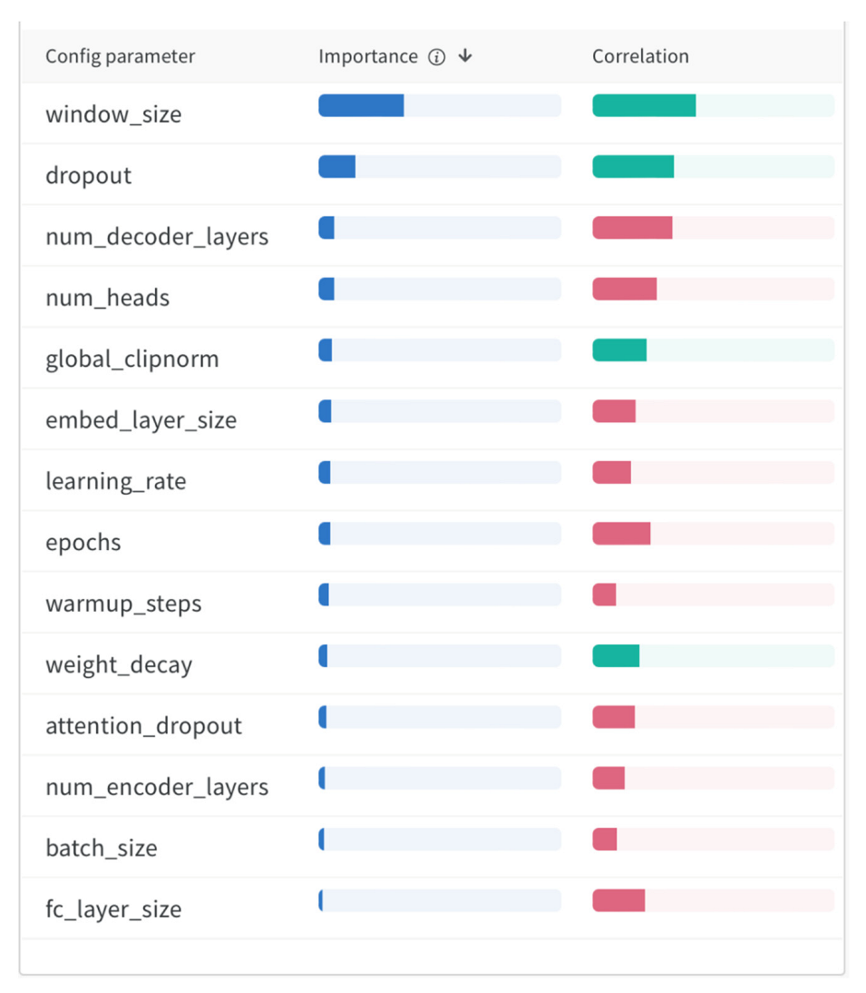
In Figure 11, we can see the significance of the hyperparameters in affecting the best validation mean squared error metric and also their correlation with this metric. The hyperparameters are ranked in order of importance from most significant to least significant. The green correlation represents a positive relationship, which means that as the value of the hyperparameter increases, the error of the model increases. A red correlation represents the opposite, and thus the best mean squared error metric decreases as the value of the hyperparameter increases.
3. Results
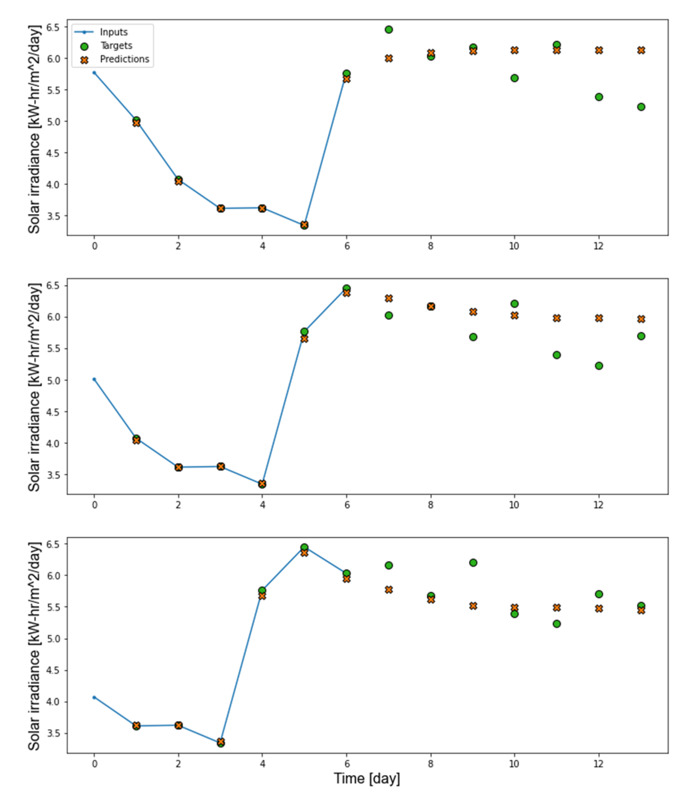
Figure 12 shows the solar irradiance prediction for 7 days ahead. The orange points represent the predicted solar irradiance values by the model, and the green points depict the measured values from the dataset. As can be seen in the graph, the model is, on the whole, accurate in predicting the future. It was also found that it is not advisable to make longer predictions than the specified window size of the model.
The results show that the smallest average solar irradiance prediction error is about 131.49326 Wh/m2/day, which is a good result when the average daily solar irradiance is 5.3070946 kWh/m2/day (the error is less than 2.5% of the mean solar irradiance). The MAPE error results are presented in Table 1.
As shown in Table 1, the model proposed in this paper achieved a smaller worst-case error than those of the competing models. It must be emphasized that for the proposed model, Table 1 shows the result for the region, where the solar irradiance proved to be the most difficult to predict. It is the densely populated Chennai Metropolitan Area located on the east coast of India with a tropical savanna climate where the temperature reaches 45 °C in extremes. When comparing results across the various areas predicted by the proposed model, Bitta Solar Power Plant, located in a sparsely populated area in western India off the Arabian Sea coast, proved the easiest to predict with a MAPE error of only 1.86%.
Optimal Hyperparameters
The optimization of the model hyperparameters was performed through the W&B Sweep environment. Tuning of the hyperparameters was aimed at minimizing the validation mean squared error, i.e., the most optimal model settings in terms of minimizing this metric were sought. The resulting model (see Table 2) contained large numbers of both encoder and decoder blocks due to the amount of training data producing the smallest overfit. This advantageous result could also be due to the appropriate setup and use of the dropout technique as well as residual connection [33,34].
4. Discussion
Currently, the decoder (simulator) part of the model is used to predict the future in the form of daily data. In the future, a partition of the latent space among several independent decoder blocks will be possible. In this way, each of the independent decoder blocks could predict a different time unit. In addition to daily data, NASA POWER also provides monthly data containing the annual average and hourly data. The disadvantage of hourly data is that it does not contain regional data and thus cannot be used on the encoder input side. Using independent decoder blocks architecture, the Transformer can be used to aggregate gradients from multiple nodes (decoders) in the encoder part, thus strengthening the accuracy of the training process of the encoder part, assuming there is a replenishment of data in each time category. It is also a prerequisite to have synchronized windows across all time categories.
5. Conclusions
The results show that it is advantageous to use space–time bonds between features as well as point and regional data in solar irradiance prediction. The paper also resulted in a model capable of predicting a specified number of timesteps ahead based on historical data as well as its own prediction of the future. The Transformer model proved to be a convenient solution not only for tasks dealing with images or natural language but also for tasks related to predicting the future values of a physical quantity. The basis for this method is a rich knowledge of historical data, which the model can draw on during learning and thus adapt not only to the average weather. Given a sufficiently long time, the dataset could include several dramatic natural events, such as volcanic activity, large-scale fires, or global warming. Another advantage of the Transformer model proved to be the coupling of regional data to predict point (target) solar irradiance. This feature of the proposed model is based on the idea of translation from one natural language to another natural language. Moreover, the property of matching words with the same or similar meaning from two different dictionaries is reflected by linking the local regions across India according to their influence in predicting future solar irradiance. The Transformer model has proved to be a suitable solution for finding the correlations, with the advantage that its computation is massively parallelized.
Supplementary Materials
The Solar Transformer code and further description can be downloaded at: https://github.com/markub3327/Solar-Transformer (accessed on 1 July 2022). The NASA Power bot code and further description can be downloaded at: https://github.com/markub3327/NASA-POWER-BOT (accessed on 1 July 2022). The online interactive charts at: https://wandb.ai/markub/solar-transformer?workspace=user-markub (accessed on 1 July 2022).
Author Contributions
Conceptualization, I.D.L. and J.P.; methodology, M.K.; software, M.K.; validation, M.K.; formal analysis, J.P.; investigation, M.K.; resources I.D.L.; data curation, M.K.; writing—original draft preparation, M.K.; writing—review and editing, J.P.; visualization, M.K.; supervision, I.D.L. and J.P.; project administration, I.D.L.; funding acquisition, I.D.L. All authors have read and agreed to the published version of the manuscript.
Funding
This research was funded by the Cultural and Educational Grant Agency MŠVVaŠ SR, grant number KEGA 012UCM-4/2021, and by the Slovak Research and Development Agency, grant number APVV-17-0116.
Institutional Review Board Statement
Not applicable.
Informed Consent Statement
Not applicable.
Data Availability Statement
Not applicable.
Conflicts of Interest
The authors declare no conflict of interest.
References
- Ariga, K.; Zheng, K. Forecasting Solar Irradiance from Time Series with Exogenous Information. Available online: https://kaiyuzheng.me/projects/projects/ForecastingSolar546.pdf (accessed on 24 August 2022).
- NASA Power Project. Available online: https://power.larc.nasa.gov (accessed on 1 August 2022).
- Zelikman, E.; Zhou, S.; Irvin, J.; Raterink, C.; Sheng, H.; Avati, A.; Kelly, J.; Rajagopal, R.; Ng, A.Y.; Gagne, D. Short–term solar irradiance forecasting using calibrated probabilistic models. arXiv 2020, arXiv:2010.04715. [Google Scholar]
- Vaswani, A.; Shazeer, N.; Parmar, N.; Uszkoreit, J.; Jones, L.; Gomez, A.N.; Kaiser, Ł.; Polosukhin, I. Attention is all you need. Adv. Neural Inf. Process. Syst. 2017, 30. Available online: https://proceedings.neurips.cc/paper/2017/file/3f5ee243547dee91fbd053c1c4a845aa-Paper.pdf (accessed on 1 August 2022).
- TensorFlow Framework. Available online: https://www.tensorflow.org (accessed on 1 August 2022).
- Brahma, B.; Wadhvani, R. Solar irradiance forecasting based on deep learning methodologies and multi–site data. Symmetry 2020, 12, 1830. [Google Scholar] [CrossRef]
- Alzahrani, A.; Shamsi, P.; Dagli, C.; Ferdowsi, M. Solar irradiance forecasting using deep neural networks. Procedia Comput. Sci. 2017, 114, 304–313. Available online: https://www.sciencedirect.com/science/article/pii/S1877050917318392?ref=cra_js_challenge&fr=RR-1 (accessed on 1 August 2022). [CrossRef]
- Alharbi, F.R.; Csala, D. Wind Speed and Solar Irradiance Prediction Using a Bidirectional Long Short-Term Memory Model Based on Neural Networks. Energies 2021, 14, 6501. Available online: https://www.mdpi.com/1996-1073/14/20/6501 (accessed on 1 August 2022). [CrossRef]
- Premalatha, N.; Valan Arasu, A. Prediction of solar radiation for solar systems by using ANN models with different back propagation algorithms. J. Appl. Res. Technol. 2016, 14, 206–214. Available online: https://www.elsevier.es/en-revista-journal-applied-research-technology-jart-81-pdf-S1665642316300438 (accessed on 1 August 2022). [CrossRef]
- Zafar, R.; Vu, B.H.; Husein, M.; Chung, I.Y. Day–Ahead Solar Irradiance Forecasting Using Hybrid Recurrent Neural Network with Weather Classification for Power System Scheduling. Appl. Sci. 2021, 11, 6738. Available online: https://www.mdpi.com/2076-3417/11/15/6738 (accessed on 1 August 2022). [CrossRef]
- Wang, F.; Yu, Y.; Zhang, Z.; Li, J.; Zhen, Z.; Li, K. Wavelet decomposition and convolutional LSTM networks based improved deep learning model for solar irradiance forecasting. Appl. Sci. 2018, 8, 1286. Available online: https://www.mdpi.com/2076-3417/8/8/1286 (accessed on 1 August 2022). [CrossRef]
- Wang, F.; Mi, Z.; Su, S.; Zhao, H. Short-term solar irradiance forecasting model based on artificial neural network using statistical feature parameters. Energies 2012, 5, 1355–1370. Available online: https://www.mdpi.com/1996-1073/5/5/1355/htm (accessed on 1 August 2022). [CrossRef]
- Husein, M.; Chung, I.Y. Day–ahead solar irradiance forecasting for microgrids using a long short–term memory recurrent neural network: A deep learning approach. Energies 2019, 12, 1856. Available online: https://www.mdpi.com/1996-1073/12/10/1856 (accessed on 1 August 2022). [CrossRef]
- Mendonça de Paiva, G.; Pires Pimentel, S.; Pinheiro Alvarenga, B.; Gonçalves Marra, E.; Mussetta, M.; Leva, S. Multiple site intraday solar irradiance forecasting by machine learning algorithms: MGGP and MLP neural networks. Energies 2020, 13, 3005. Available online: https://www.mdpi.com/1996-1073/13/11/3005 (accessed on 1 August 2022). [CrossRef]
- Park, S.; Kim, Y.; Ferrier, N.J.; Collis, S.M.; Sankaran, R.; Beckman, P.H. Prediction of solar irradiance and photovoltaic solar energy product based on cloud coverage estimation using machine learning methods. Atmosphere 2021, 12, 395. Available online: https://www.mdpi.com/2073-4433/12/3/395/htm (accessed on 1 August 2022). [CrossRef]
- Yang, L.; Gao, X.; Hua, J.; Wu, P.; Li, Z.; Jia, D. Very short-term surface solar irradiance forecasting based on FengYun–4 geostationary satellite. Sensors 2020, 20, 2606. Available online: https://www.mdpi.com/1424-8220/20/9/2606/htm (accessed on 1 August 2022). [CrossRef] [PubMed]
- Solar Power by Country. Available online: https://worldpopulationreview.com/country-rankings/solar-power-by-country (accessed on 18 August 2022).
- Srivastava, R.; Tiwari, A.N.; Giri, V.K. Forecasting of solar radiation in India using various ANN models. In Proceedings of the 2018 5th IEEE Uttar Pradesh Section International Conference on Electrical, Electronics and Computer Engineering (UPCON), Gorakhpur, India, 2–4 November 2018; pp. 1–6. Available online: https://www.researchgate.net/publication/331421649_Forecasting_of_Solar_Radiation_in_India_Using_Various_ANN_Models (accessed on 18 August 2022).
- Mitra, I.; Heinemann, D.; Ramanan, A.; Kaur, M.; Sharma, S.K.; Tripathy, S.K.; Roy, A. Short-term PV power forecasting in India: Recent developments and policy analysis. Int. J. Energy Environ. Eng. 2022, 13, 515–540. Available online: https://link.springer.com/article/10.1007/s40095-021-00468-z (accessed on 18 August 2022). [CrossRef]
- Mukherjee, A.; Ain, A.; Dasgupta, P. Solar irradiance prediction from historical trends using deep neural networks. In Proceedings of the 2018 IEEE International Conference on Smart Energy Grid Engineering (SEGE), Oshawa, ON, Canada, 12–15 August 2018; pp. 356–361. Available online: https://ieeexplore.ieee.org/document/8499394 (accessed on 18 August 2022).
- Rezatofighi, H.; Tsoi, N.; Gwak, J.; Sadeghian, A.; Reid, I.; Savarese, S. Generalized intersection over union: A metric and a loss for bounding box regression. In Proceedings of the IEEE/CVF Conference on Computer Vision and Pattern Recognition, Long Beach, CA, USA, 15–20 June 2019; pp. 658–666. Available online: https://www.computer.org/csdl/proceedings-article/cvpr/2019/329300a658/1gyrWyRZ0k0 (accessed on 1 August 2022).
- Chollet, F. Deep Learning with Python; Simon and Schuster: New York, NY, USA, 2021; ISBN 978-80-271-2751-1. [Google Scholar]
- Keisler, R. Forecasting Global Weather with Graph Neural Networks. arXiv 2022, arXiv:2202.07575. [Google Scholar]
- Meteorological Wind Direction. Available online: http://tornado.sfsu.edu/geosciences/classes/m430/Wind/WindDirection.html (accessed on 1 August 2022).
- Dosovitskiy, A.; Beyer, L.; Kolesnikov, A.; Weissenborn, D.; Zhai, X.; Unterthiner, T.; Dehghani, M.; Minderer, M.; Heigold, G.; Gelly, S.; et al. An image is worth 16x16 words: Transformers for image recognition at scale. arXiv 2020, arXiv:2010.11929. [Google Scholar]
- Bao, H.; Dong, L.; Wei, F. Beit: Bert pre–training of image transformers. arXiv 2021, arXiv:2106.08254. [Google Scholar]
- Loshchilov, I.; Hutter, F. SGDR: Stochastic Gradient Descent with Warm Restarts. arXiv 2016, arXiv:1608.03983. [Google Scholar]
- Chen, P.; Chen, G.; Zhang, S. Log Hyperbolic Cosine Loss Improves Variational Auto-Encoder. 2018. Available online: https://openreview.net/forum?id=rkglvsC9Ym (accessed on 1 August 2022).
- Rehman, S.; Mohandes, M. Artificial neural network estimation of global solar radiation using air temperature and relative humidity. Energy Policy 2008, 36, 571–576. Available online: https://www.sciencedirect.com/science/article/abs/pii/S0301421507004284?via%3Dihub (accessed on 1 August 2022). [CrossRef]
- Sözen, A.; Arcaklıoğlu, E.; Özalp, M.; Çağlar, N. Forecasting based on neural network approach of solar potential in Turkey. Renew. Energy 2005, 30, 1075–1090. Available online: https://www.sciencedirect.com/science/article/abs/pii/S0960148104003702?via%3Dihub (accessed on 1 August 2022). [CrossRef]
- Sözen, A.; Arcaklioǧlu, E.; Özalp, M.; Kanit, E.G. Use of artificial neural networks for mapping of solar potential in Turkey. Appl. Energy 2004, 77, 273–286. Available online: https://www.sciencedirect.com/science/article/abs/pii/S0306261903001375?via%3Dihub (accessed on 1 August 2022). [CrossRef]
- Theocharides, S.; Makrides, G.; Livera, A.; Theristis, M.; Kaimakis, P.; Georghiou, G.E. Day-ahead photovoltaic power production forecasting methodology based on machine learning and statistical post-processing. Appl. Energy 2020, 268, 115023. Available online: https://www.sciencedirect.com/science/article/pii/S0306261920305353 (accessed on 1 August 2022).
- Srivastava, N.; Hinton, G.; Krizhevsky, A.; Sutskever, I.; Salakhutdinov, R. Dropout: A simple way to prevent neural networks from overfitting. J. Mach. Learn. Res. 2014, 15, 1929–1958. Available online: https://jmlr.org/papers/volume15/srivastava14a/srivastava14a.pdf (accessed on 1 August 2022).
- He, K.; Zhang, X.; Ren, S.; Sun, J. Deep residual learning for image recognition. In Proceedings of the IEEE Conference on Computer Vision and Pattern Recognition, Las Vegas, NV, USA, 27–30 June 2016; pp. 770–778. Available online: https://arxiv.org/abs/1512.03385?context=cs (accessed on 1 August 2022).
- Loshchilov, I.; Hutter, F. Decoupled weight decay regularization. arXiv 2017, arXiv:1711.05101. [Google Scholar]
Figure 1.
Visualization of the thinning of regions on the world map from Google Earth. (a) Initial map of regions on the left. (b) On the right, the resulting thinned-out map of the regions.
Figure 1.
Visualization of the thinning of regions on the world map from Google Earth. (a) Initial map of regions on the left. (b) On the right, the resulting thinned-out map of the regions.

Figure 2.
Visualization of visible correlations between weather variables and solar irradiance.

Figure 3.
Visualization of the frequency of occurrences wind of given speed in given directions.

Figure 4.
Visualization of the frequency of occurrences of wind characteristics by wind vector.

Figure 5.
Transformer model for Solar irradiance.

Figure 6.
Principle of prediction for the latent space.

Figure 7.
Principle of prediction for the future solar irradiance.

Figure 8.
Cosine similarity of temporal position embedding. (a) The left side shows the position embedding for the encoder part. (b) The right side shows the position embedding for the decoder part.
Figure 8.
Cosine similarity of temporal position embedding. (a) The left side shows the position embedding for the encoder part. (b) The right side shows the position embedding for the decoder part.

Figure 9.
Cosine similarity of spatial position embedding. (a) The left side shows the position embedding for the encoder block. (b) The right side shows position embedding for the decoder block.
Figure 9.
Cosine similarity of spatial position embedding. (a) The left side shows the position embedding for the encoder block. (b) The right side shows position embedding for the decoder block.

Figure 10.
Cosine similarity between 0th patch and other patches on the world map from Google Earth.
Figure 10.
Cosine similarity between 0th patch and other patches on the world map from Google Earth.

Figure 11.
Significance of the hyperparameters and their correlation with the best validation mean squared error metric.
Figure 11.
Significance of the hyperparameters and their correlation with the best validation mean squared error metric.

Figure 12.
Example of 0th patch 7-day-ahead prediction.


Table 1.
Mean absolute percentage error results.
| Paper | Location | MAPE (%) |
|---|---|---|
| [29] | Abha (Saudi Arabia) | 11.8 |
| [30] | Sirt (Turkey) | 6.78 |
| [31] | Mugla (Turkey) | 6.73 |
| [32] | Cyprus and USA | 4.7 |
| [9] | Mumbai (India) | 4.24 |
| This paper | Chennai Metropolitan Area (India) | 3.45 |
Table 2.
The optimized hyperparameters.
| Name | Description | Value |
|---|---|---|
| Attention dropout | Dropout applied to the attention matrix | 0.25 |
| Batch size | Number of examples per one training batch | 32 |
| Dropout | Dropout applied between hidden layers | 0.15 |
| Embed layer size | Size of the Key, Value, Query matrices | 64 |
| Epochs | Number of training epochs | 1000 |
| FC layer size | Size of the fully connected feed-forward network block | 256 |
| Global clipnorm | Global clipnorm for the optimizer | 2 |
| Learning rate | Learning rate for the optimizer | 0.005 |
| No. decoder layers | Number of decoder blocks | 6 |
| No. encoder layers | Number of encoder blocks | 3 |
| No. heads | Number of heads in every Multi-head Attention block in the model | 6 |
| Optimizer | Optimizer used during training | AdamW [35] |
| Warmup steps | Warmup steps of the learning rate cosine scheduler | 70 |
| Weight decay | Weight decay for the optimizer | 0.00001 |
| Window size | Windows size defines the size of known history | 7 |
Publisher’s Note: MDPI stays neutral with regard to jurisdictional claims in published maps and institutional affiliations. |
© 2022 by the authors. Licensee MDPI, Basel, Switzerland. This article is an open access article distributed under the terms and conditions of the Creative Commons Attribution (CC BY) license (https://creativecommons.org/licenses/by/4.0/).
Share and Cite
MDPI and ACS Style
Pospíchal, J.; Kubovčík, M.; Dirgová Luptáková, I. Solar Irradiance Forecasting with Transformer Model. Appl. Sci. 2022, 12, 8852. https://doi.org/10.3390/app12178852
AMA Style
Pospíchal J, Kubovčík M, Dirgová Luptáková I. Solar Irradiance Forecasting with Transformer Model. Applied Sciences. 2022; 12(17):8852. https://doi.org/10.3390/app12178852
Chicago/Turabian StylePospíchal, Jiří, Martin Kubovčík, and Iveta Dirgová Luptáková. 2022. "Solar Irradiance Forecasting with Transformer Model" Applied Sciences 12, no. 17: 8852. https://doi.org/10.3390/app12178852
Note that from the first issue of 2016, this journal uses article numbers instead of page numbers. See further details here.