
Analysis of a Stochastic SICR Epidemic Model Associated with the Lévy Jump


1
Department of Mathematics and Statistics, University of Victoria, Victoria, BC V8W 3R4, Canada
2
Department of Medical Research, China Medical University Hospital, China Medical University, Taichung 40402, Taiwan
3
Department of Mathematics and Informatics, Azerbaijan University, 71 Jeyhun Hajibeyli Street, AZ1007 Baku, Azerbaijan
4
Section of Mathematics, International Telematic University Uninettuno, I-00186 Rome, Italy
5
Laboratory of Systems Modelization and Analysis for Decision Support, National School of Applied Sciences, Hassan First University of Settat, Berrechid 26100, Morocco
*
Author to whom correspondence should be addressed.
Appl. Sci. 2022, 12(17), 8434; https://doi.org/10.3390/app12178434
Submission received: 26 July 2022
/
Revised: 17 August 2022
/
Accepted: 19 August 2022
/
Published: 24 August 2022
(This article belongs to the Special Issue Quantum Analysis and Fractional Calculus and Their Multi-Disciplinary Applications)
Abstract
:We propose and study a Susceptible-Infected-Confined-Recovered (SICR) epidemic model. For the proposed model, the driving forces include (for example) the Brownian motion processes and the jump Lévy noise. Usually, in the existing literature involving epidemiology models, the Lévy noise perturbations are ignored. However, in view of the presence of strong fluctuations in the SICR dynamics, it is worth including these perturbations in SICR epidemic models. Quite frequently, this results in several discontinuities in the processes under investigation. In our present study, we consider our SICR model after justifying its used form, namely, the component related to the Lévy noise. The existence and uniqueness of a global positive solution is established. Under some assumptions, we show the extinction and the persistence of the infection. In order to give some numerical simulations, we illustrate a new numerical method to validate our theoretical findings.
Keywords:
Susceptible-Infected-Confined-Recovered (SICR) epidemic model; Lévy jump; stochastic model; Brownian motion; extinction; persistenceMSC:
Primary 60H10; 65D25; 92B05; Secondary 68Q871. Introduction
In a large variety of ecosystems and in humans, which are the most affected species, epidemics are known to pose a significant threat to living organisms. Every year, millions of humans die from epidemics, which has motivated researchers in mathematical and biological sciences to develop control and mitigation strategies in the fight against epidemic diseases. Using various mathematical modeling techniques, epidemiologists have gained deeper insights into the dynamics by using this mathematical and cost-effective analytical setup, whereas traditional experimental techniques are time-consuming and more expensive. This has encouraged many mathematicians and biologists to develop competent epidemic models that can present a vivid picture of the reality (see, for details, [1,2,3,4,5,6]).
The first SIR model describing the dynamics of the three principal populations: the susceptible , the infected and the recovered , was studied by Kermack and McKendricks in 1927 (see [7]). Their proposed model played a cruciel role in initianting different research works in the field of disease dynamics. Based upon the natural history of hepatitis C, a recent study proposed a Susceptible–Infectious–Chronic–Recovered (SICR) type model (see [8]).
A natural phenomenon is always affected by environmental factors that can aggravate or mitigate the spread of the epidemic. The stochastic quantification of several real-life phenomena has been immensely helpful in understanding the random nature of their incidence or occurrence. It has also helped to find solutions to those problems that arise from it, either in the form of minimizing their undesirability or maximizing their rewards. In addition, infectious diseases are subject to chance and uncertainty in terms of the normal progression of the infection. Therefore, stochastic models are more suitable when compared to deterministic models, keeping in view the fact that stochastic systems consider not only the moving mean, but also the standard deviation behavior around it. On the other hand, deterministic systems generate similar results for fixed initial values, but stochastic systems may give different predicted results. Several stochastic infection models describing the effect of the Brownian motion on viral dynamics have been developed in the literature (see, for example, [9,10,11,12,13]; see also [14]).
Motivated essentially by the above-mentioned and other recent developments (see [15,16,17,18,19,20,21,22,23,24,25,26,27,28,29,30,31,32]), we propose here a mathematical model for the transmission of an SICR model. Our goal is to show the effect of the Lévy jump in population dynamics, in which the Lévy noise is used to describe contingency and outburst. It will, therefore, be interesting to consider the following stochastic model jointly driven by white noise and Lévy noise:
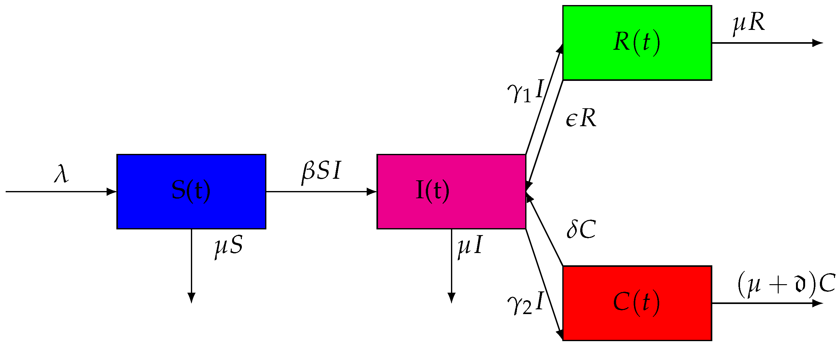
where denotes the number of susceptible individuals at time t. The infected individuals with no clinical symptoms (that is, the virus is living or developing in the individuals, but without producing symptoms or only mild ones) are able to transmit the infection to other individuals . The infected individuals under treatment (that is, those in the so-called chronic stage) with a viral load remaining low , and denotes the number of the recovered individuals at time t. The parameters of the SICR model (1) are given in Table 1 and the two-strain SEIR diagram is illustrated in Figure 1. Moreover, is a standard Brownian motion with intensity defined on a complete filtered probability space:
with the filtration satisfying the usual conditions. We denote by , , and the left limits of , , and , respectively. is a Poisson counting measure with the stationary compensator given by
where is defined on a measurable subset U of the non-negative half-line with . represents the jump intensity.
2. Existence and Uniqueness of the Global Positive Solution
In this section, we first define as follows:
and we consider the following assumption:
Theorem 1.
Moreover, each of the following inequalities holds true:
and
Proof.
Since the drift and the diffusion are local Lipschitzian, and in view of the initial condition we prove the existence and uniqueness of the local solution for , where is the explosion time.
In order to prove that this solution is global, we define the stopping time given by
If we suppose that , then , so there exist and such that .
Consider the function V on defined by
Using the Itô’s formula, we get
where
Noting that from Assumption (A), this fact implies that
Since and are nonpositive functions, we find that
which, upon integrating from 0 to t, yields
Now, by using the continuity property, some components of will be equal to 0, so we obtain
For , we get
which contradicts our hypothesis. Thus, clearly, we have shown that the solution of (1) is global.
Next, we will prove the boundedness of the solution. The equation of the system (1) implies that
where
Therefore, we have
so that
and
Using the same technique as above, we get
This proves the boundedness. □
The above result shows the biologically well-posedness of our model and also that the solution is ultimately bounded such that
and
3. Extinction of the Infection
In this section, we will prove the extinction of the infection under some sufficient condition. We first define by
Theorem 2.
If then when a.s.
Proof.
Let
Then, by using Itô’s formula, we obtain
with
so we have
so that
Therefore, we get
If we now define by
then
Thus, by using the fact that the solution of the system (1) is bounded and also the strong law of large numbers theorem for martingales, we have (see [33])
so that
So, if
when , then when a.s. □
This result shows that the disease dies out when we have the critical threshold of a possibly greater amplitude of the volatility , which is described as follows:
4. Persistence in the Mean
Firstly, we define
then the persistence in the mean of is defined as follows:
Now, we will give some condition to prove the persistence of , , and in the mean. For this purpose we define by
Theorem 3.
and
Proof.
Thus, by the boundedness of solution and the strong law of large numbers for the martingales, we obtain
Next, by integrating the second equation of the system (1) from 0 to t and dividing both sides by t, we obtain
Using the Itô’s formula on , we have
and
Now, if we sum
by using the positivity and the boundedness of the solution as well as the strong law of large numbers for the martingales, we find that
Hence, we have
Consequently, the persistence in the mean of is proved.
This last equation of the model (1) implies that
Therefore, we finally obtain
□
The theorem involving the persistence in the mean has been proved under the following sufficient condition:
This means that, with an adopted smallest magnitude of volatility , the model is persistent in the mean.
5. Numerical Results
In order to illustrate the numerical simulations of the model (1), we consider the following problem:
The solution of the system (2) will now be given by
The Milsteins Higher Order Method consists of approximating Part 1 in the system (2) in the following form:
About the approximation of Part 2, we have two cases. Consider any infinitesimal interval .
There is no jump point in this interval:
If there is only one jump point then
so that
Therefore, the Milsteins Higher Order Method of the system (2) will be given by
We now use the previous method to solve the system (1).
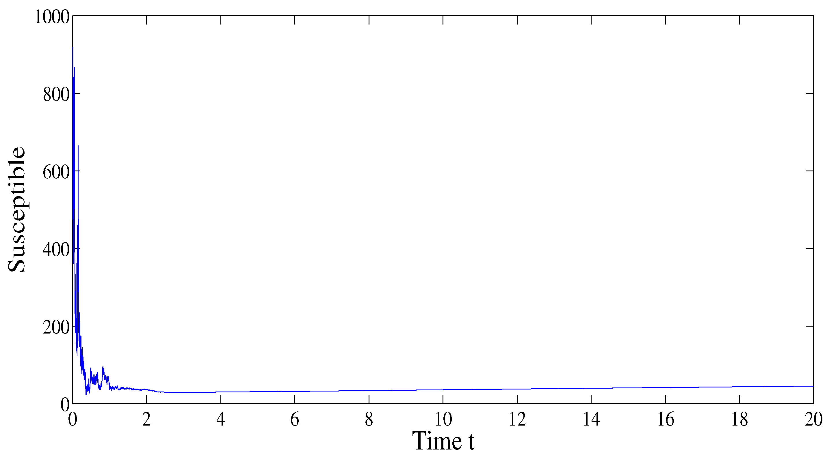
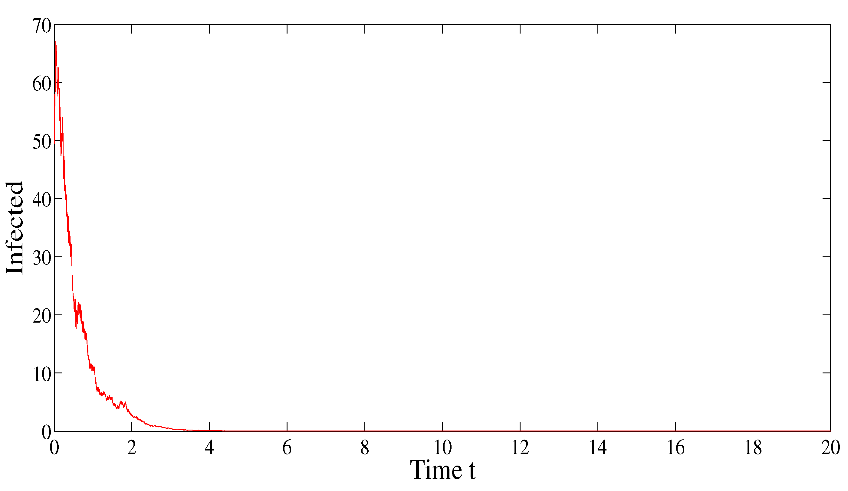
Figure 2 and Figure 3 show the dynamics of the susceptible population for the case of the extinction of the infection. From these figures, we observe clearly that the infected compartment converges to 0. It should be noted that, in this case, the susceptible class increases to attain their maximum, which means the the disease dies out. This is consistent with our theoretical results for the extinction of the infection.
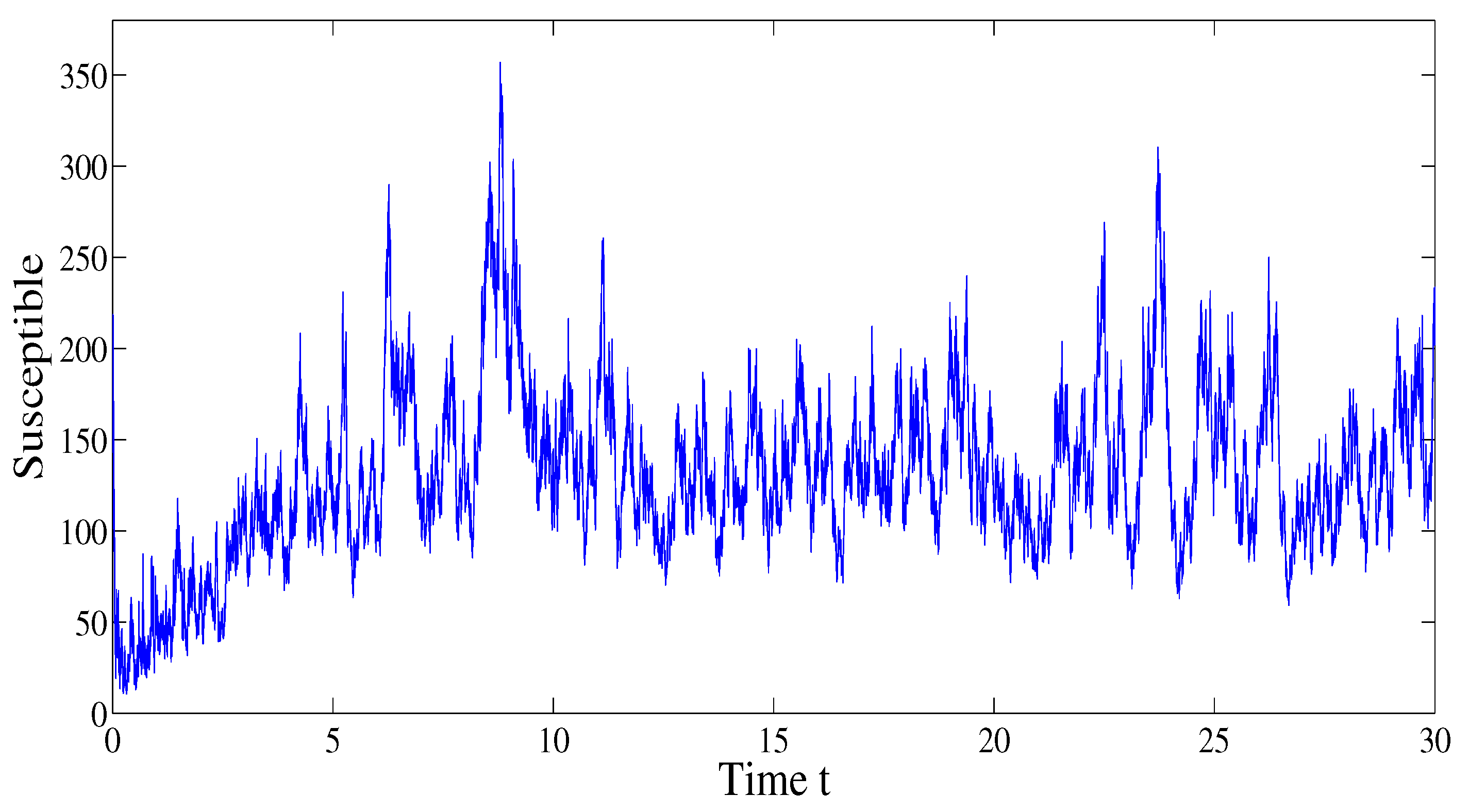
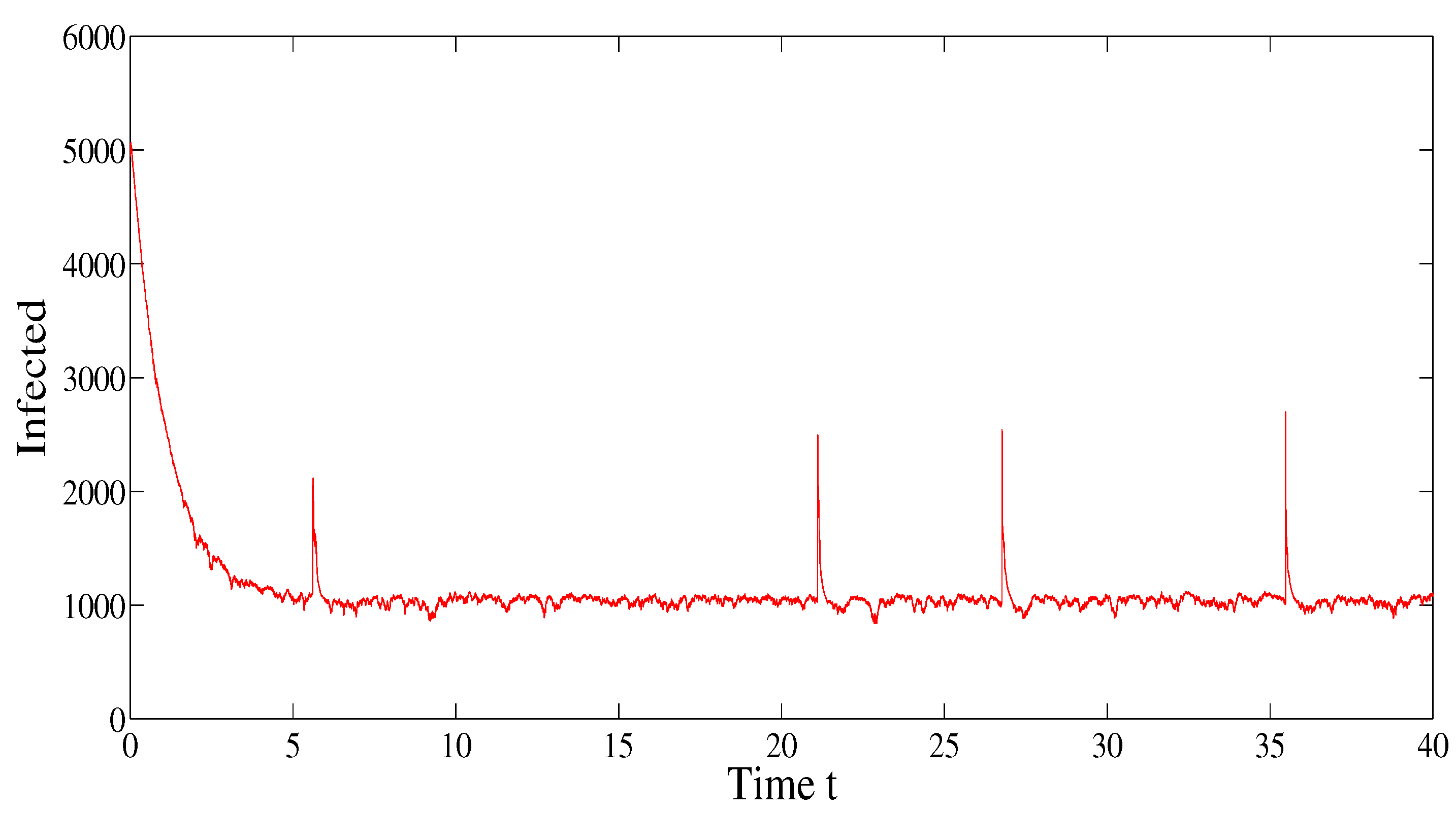
The behavior of the infection for both the infected and susceptible population with the Lévy jump process is graphically illustrated in Figure 4 and Figure 5 in the case of the persistence of the infection. In this epidemic scenario, we note from all of the four SICR compartments, that is, the infected, the susceptible, the chronic sub-population and the recovered, that the infection persists. This shows that our theoretical and numerical results are compatible.
6. Conclusions
In our present investigation, we have considered the stochastic epidemic SICR model which is driven by the Brownian motion and the Lévy noise jointly so as to better describe the sudden social fluctuations. We have also performed some adequate numerical simulations not only to support our theoretical results, but also for predicting the asymptotic behavior of the solutions of the corresponding system in this study. More precisely, first of all, by using the Lyapunov analysis method, we have demonstrated the existence and uniqueness of the derived solutions. In addition, we have shown the positivity and the boundedness:
and
The extinction of the infection is established with a critical threshold of a possible greater amplitude of the volatility , which is described as follows:
The persistence of the infection has been proved under the following sufficient condition:
Finally, we have constructed a modified Milsteins Higher Order Method, which is implemented in order to validate our theoretical findings in relation to the model considered, with the aim to provide additional information to help the decision makers choose a good disease control strategy. On the one hand, we have decreased or increased the intensity of fluctuations. On the other hand, we have considered the effect of the Lévy noise in the development of the system variables. In possible sequels to our investigation in this paper, one can extend the model (1) to various fractional-order models, which are based upon several operators of fractional derivatives such as those known as the Riemann–Liouville, Liouville–Caputo and other fractional derivatives (see, for example, [34,35]) and also extend our model to an impulsive model such as that considered in [36].
Author Contributions
Formal analysis, H.M.S.; Investigation, H.M.S. and J.D.; Methodology, J.D.; Supervision, H.M.S.; Writing—original draft, J.D.; Writing—review & editing, H.M.S. All authors have read and agreed to the published version of the manuscript.
Funding
This research received no external funding.
Institutional Review Board Statement
Not applicable.
Informed Consent Statement
Not applicable.
Data Availability Statement
Not applicable.
Conflicts of Interest
The authors declare no conflict of interest.
References
- World Health Organization HIV/AIDS Key Facts. November 2017. Available online: http://www.who.int/mediacentre/factsheets/fs360/en/index.html (accessed on 5 July 2022).
- Allali, K.; Danane, J.; Kuang, Y. Global analysis for an HIV infection model with CTL immune response and infected cells in eclipse phase. Appl. Sci. 2017, 7, 861. [Google Scholar] [CrossRef] [Green Version]
- Korobeinikov, A. Global properties of basic virus dynamics models. Bull. Math. Biol. 2004, 66, 879–883. [Google Scholar] [CrossRef] [PubMed]
- Nowak, M.A.; Bangham, C.R.M. Population dynamics of immune responses to persistent viruses. Science 1996, 272, 74–79. [Google Scholar] [CrossRef] [PubMed] [Green Version]
- Smith, H.L.; De Leenheer, P. Virus dynamics: A global analysis. SIAM J. Appl. Math. 2003, 63, 1313–1327. [Google Scholar] [CrossRef]
- Sun, Q.; Min, L.; Kuang, Y. Global stability of infection-free state and endemic infection state of a modified human immunodeficiency virus infection model. IET Syst. Biol. 2015, 9, 95–103. [Google Scholar] [CrossRef] [PubMed] [Green Version]
- Kermack, W.O.; McKendrick, A.G. A contribution to the mathematical theory of epidemics. Proc. R. Soc. Lond. Ser. A Math. Phys. Engrg. Sci. 1927, 115, 700–721. [Google Scholar]
- Qiao, M.; Liu, A.; Forys, U. Qualitative analysis of the SICR epidemic model with impulsive vaccinations. Math. Methods Appl. Sci. 2013, 36, 695–706. [Google Scholar] [CrossRef]
- Rajaji, R.; Pitchaimani, M. Analysis of stochastic viral infection model with immune impairment. Int. J. Appl. Comput. Math. 2017, 3, 3561–3574. [Google Scholar] [CrossRef]
- Akdim, K.; Ez-Zetouni, A.; Danane, J.; Allali, K. Stochastic viral infection model with lytic and nonlytic immune responses driven by Lévy noise. Phys. A Stat. Mech. Its Appl. 2020, 549, 124367. [Google Scholar] [CrossRef]
- Mahrouf, M.; El-Mehdi, L.; Mehdi, M.; Hattaf, K.; Yousfi, N. A stochastic viral infection model with general functional response. Nonlinear Anal. Differ. Equ. 2016, 4, 435–445. [Google Scholar] [CrossRef]
- Pitchaimani, M.; Brasanna, D.M. Effects of randomness on viral infection model with application. IFAC J. Syst. Control 2018, 6, 53–69. [Google Scholar] [CrossRef]
- Zhang, Q.; Zhou, K. Stationary distribution and extinction of a stochastic SIQR model with saturated incidence rate. Math. Probl. Engrg. 2019, 2019, 3575410. [Google Scholar] [CrossRef]
- Mao, X. Stochastic Differential Equations and Their Applications; Horwood Publishing Series in Mathematics and Applications; Horwood Publishing Limited: Chichester, UK, 1997; 2nd ed.; Woodhead Publishing Limited: Oxford, UK; Cambridge, UK; Philadelphia, PA, USA; New Delhi, India, 2011. [Google Scholar]
- Weiss, R.A. How does HIV cause AIDS? Science 1993, 260, 1273–1279. [Google Scholar] [CrossRef] [PubMed]
- Bao, J.; Mao, X.; Yin, G.; Yuan, C. Competitive Lotka-Volterra population dynamics with jumps. Nonlinear Anal. 2011, 74, 6601–6616. [Google Scholar] [CrossRef] [Green Version]
- Momani, S.; Kumar, R.; Srivastava, H.M.; Kumar, S.; Hadid, S. A chaos study of fractional SIR epidemic model of childhood diseases. Results Phys. 2021, 27, 104422. [Google Scholar] [CrossRef]
- Srivastava, H.M.; Günerhan, H. Analytical and approximate solutions of fractional-order susceptible-infected-recovered epidemic model of childhood disease. Math. Methods Appl. Sci. 2019, 42, 935–941. [Google Scholar] [CrossRef]
- Bao, J.; Yuan, C. Stochastic population dynamics driven by Lévy noise. J. Math. Anal. Appl. 2012, 391, 363–375. [Google Scholar] [CrossRef] [Green Version]
- Blanttner, W.; Gallo, R.C.; Temin, H.M. HIV causes aids. Science 1988, 241, 515–516. [Google Scholar] [CrossRef]
- Srivastava, H.M.; Dubey, R.S.; Jain, M. A study of the fractional-order mathematical model of diabetes and its resulting complications. Math. Methods Appl. Sci. 2019, 42, 4570–4583. [Google Scholar] [CrossRef]
- Srivastava, H.M. Diabetes and its resulting complications: Mathematical modeling via fractional calculus. Public Health Open Access 2020, 4, 2. [Google Scholar] [CrossRef]
- Mahrouf, M.; Boukhouima, A.; Zine, H.; Lotfi, E.; Torres, D.F.M.; Yousfi, N. Modeling and forecasting of COVID-19 spreading by delayed stochastic differential equations. Axioms 2021, 10, 18. [Google Scholar] [CrossRef]
- Srivastava, H.M.; Saad, K.M. Numerical simulation of the fractal-fractional Ebola virus. Fractal Fract. 2020, 4, 49. [Google Scholar] [CrossRef]
- Singh, H.; Srivastava, H.M.; Hammouch, Z.; Nisar, K.S. Numerical simulation and stability analysis for the fractional-order dynamics of COVID-19. Results Phys. 2021, 20, 103722. [Google Scholar] [CrossRef] [PubMed]
- Mao, X.; Marion, G.; Renshaw, E. Environmental Brownian noise suppresses explosions in population dynamics. Stochast. Process. Appl. 2002, 97, 95–110. [Google Scholar] [CrossRef]
- Silva, C.J.; Torres, D.F.M. A SICA compartmental model in epidemiology with application to HIV/AIDS in Cape Verde. Ecol. Complex. 2017, 30, 70–75. [Google Scholar] [CrossRef] [Green Version]
- Srivastava, H.M.; Saad, K.M.; Khader, M.M. An efficient spectral collocation method for the dynamic simulation of the fractional epidemiological model of the Ebola virus. Chaos Solitons Fractals 2020, 140, 110174. [Google Scholar] [CrossRef]
- Zhang, X.; Wang, K. Stochastic model for spread of AIDS driven by Lévy noise. J. Dyn. Differ. Equ. 2015, 27, 215–236. [Google Scholar]
- Srivastava, H.M.; Saad, K.M.; Gómez-Aguilar, J.F.; Almadiy, A.A. Some new mathematical models of the fractional-order system of human immune against IAV infection. Math. Biosci. Engrg. 2020, 17, 4942–4969. [Google Scholar] [CrossRef]
- Zine, A.; Boukhouima, H.; Lotfi, E.; Mahrouf, M.; Torres, D.F.M.; Yousfi, N. A stochastic time-delayed model for the effectiveness of Moroccan COVID-19 deconfinement strategy. Math. Model. Natur. Phenom. 2020, 15, 50. [Google Scholar]
- Zou, X.; Wang, K. Numerical simulations and modeling for stochastic biological systems with jumps. Commun. Nonlinear Sci. Numer. Simulat. 2014, 19, 1557–1568. [Google Scholar]
- Lipster, R.S. A strong law of large numbers for local martingales. Stochastics 1980, 3, 217–228. [Google Scholar]
- Srivastava, H.M. An introductory overview of fractional-calculus operators based upon the Fox-Wright and related higher transcendental functions. J. Adv. Engrg. Comput. 2021, 5, 135–166. [Google Scholar] [CrossRef]
- Srivastava, H.M. Some parametric and argument variations of the operators of fractional calculus and related special functions and integral transformations. J. Nonlinear Convex Anal. 2021, 22, 1501–1520. [Google Scholar]
- Zhang, T.-W.; Zhou, J.-W.; Liao, Y.-Z. Exponentially stable periodic oscillation and Mittag-Leffler stabilization for fractional-order impulsive control neural networks with piecewise Caputo derivatives. IEEE Trans. Cybernet. 2021, 52, 9670–9683. [Google Scholar] [CrossRef] [PubMed]
Figure 1.
The diagram of the SICR model.

Figure 2.
The Susceptible population as a function of time when , , , , , , and .

Figure 3.
The infected population as a function of time when , , , , , , and .

Figure 4.
The susceptible and infected populations as functions of time when , , , , , , and .

Figure 5.
The infected population as a function of time when , , , , , , and .


Table 1.
Parameters and their meanings in the suggested SICR model.
| Parameter | Meaning |
|---|---|
| The recruitment rate | |
| Natural death rate | |
| The transmission rate | |
| The average to the infected I individuals becoming chronically infected | |
| Default treatment rate for I individuals | |
| The average of the recovered individuals returning infected | |
| The average the chronically infected individuals returning infected | |
| Death rate due to the infection in chronic stage |
Publisher’s Note: MDPI stays neutral with regard to jurisdictional claims in published maps and institutional affiliations. |
© 2022 by the authors. Licensee MDPI, Basel, Switzerland. This article is an open access article distributed under the terms and conditions of the Creative Commons Attribution (CC BY) license (https://creativecommons.org/licenses/by/4.0/).
Share and Cite
MDPI and ACS Style
Srivastava, H.M.; Danane, J. Analysis of a Stochastic SICR Epidemic Model Associated with the Lévy Jump. Appl. Sci. 2022, 12, 8434. https://doi.org/10.3390/app12178434
AMA Style
Srivastava HM, Danane J. Analysis of a Stochastic SICR Epidemic Model Associated with the Lévy Jump. Applied Sciences. 2022; 12(17):8434. https://doi.org/10.3390/app12178434
Chicago/Turabian StyleSrivastava, Hari M., and Jaouad Danane. 2022. "Analysis of a Stochastic SICR Epidemic Model Associated with the Lévy Jump" Applied Sciences 12, no. 17: 8434. https://doi.org/10.3390/app12178434
Note that from the first issue of 2016, this journal uses article numbers instead of page numbers. See further details here.