
A Proactive Approach to Extended Vehicle Routing Problem with Drones (EVRPD)


1
Department of Applied Computer Science, Kielce University of Technology, 25-314 Kielce, Poland
2
Faculty of Automatic Control, Electronics and Computer Science, Silesian University of Technology, 44-100 Gliwice, Poland
*
Author to whom correspondence should be addressed.
Appl. Sci. 2022, 12(16), 8255; https://doi.org/10.3390/app12168255
Submission received: 30 June 2022
/
Revised: 14 August 2022
/
Accepted: 16 August 2022
/
Published: 18 August 2022
(This article belongs to the Special Issue Advances in Capacitated Vehicle Routing Problem—Models, Methods, Applications and New Challenges)
Abstract
:Unmanned aerial vehicles (UAVs), also known as drones, are increasingly common and popular due to their relatively low prices and high mobility. The number of areas for their practical applications is rapidly growing. The most promising are: last-mile delivery, emergency response, the inspection of technical devices and installations, etc. In these applications, it is often necessary to solve vehicle routing problems, formulated as a variant of the vehicle routing problems with drones (VRPD). This study presents a proactive approach to a modified and extended VRPD, including: the dynamic selection of drone take-off points, bidirectional delivery (delivery and pick up), various types of shipments, allocation of shipments to drones and drones to vehicles, the selection of the optimal number of drones, etc. Moreover, a formal model of constraints and questions for the extended vehicle routing problem with drones (EVRPD) and exact and approximate methods for solving it have been proposed. The proposed model can be the basis for supporting proactive and reactive decisions regarding last-mile delivery, particularly the selection of the necessary fleet, starting points, the identification of specific shipments that prevent delivery with available resources, etc. The study also includes the results of numerous computational experiments verifying the effectiveness of the implementation methods. The time to obtain a solution is at least 20 times shorter for the proposed DGA (dedicated genetic algorithm) than for the mathematical programming solvers such as Gurobi or LINGO. Moreover, for larger-sized data instances, these solvers do not allow obtaining any solution in an acceptable time, or they obtain worse solutions.
1. Introduction
In recent years, the use of unmanned aerial vehicles (UAVs), also known as drones, has significantly increased in many areas of everyday life, such as: goods delivery, real-time monitoring, search and rescue, inspecting, remote sensing, etc. This is due to the rapid development of mobile technologies and the reduction of hardware and software costs (both purchase and operational). Logistics is the most dynamically developing and promising area for UAV application. This is the result of the rapid development of the e-commerce market, which generates a great demand for fast and cheap deliveries, especially in highly urbanized areas.
Many technology, commercial (Google, JD, Amazon) [1,2], and logistics (UPS, DHL, FedEx) companies are experimenting with the use of drones for deliveries [3,4]. These applications were initially related to the delivery of food, medicine, and water for people in danger or in areas inaccessible to other means of transportation [5], but drones have also been successfully used to deliver pizza by Flirtey, Chipotle, and Google [6].
Compared with car transportation or even couriers on scooters or bicycles, the use of drones for last-mile delivery is very attractive and promising because it has many advantages, such as: avoiding the congestion of road networks, faster and cheaper delivery, ecological aspects related to the use of electric drives (low emissions and noise), the limitation of the human factor, etc. However, some weaknesses in the use of drones for deliveries should be mentioned. The most important of them includes their limited range, low-lifting capacity, etc.
Therefore, taking all the advantages and limitations of drones into the context of delivery within the last mile, their effective use must be combined with other means of transportation, e.g., trucks [7,8]. Such deliveries are carried out together, i.e., trucks deliver the drones to the appropriate points or hubs, and from there, the drones take off with the shipments to customers and then return to the hubs. Many companies such as Amazon, Wal-Mart, Google, DHL, SF Express, etc., are starting to implement such solutions.
The key questions to be answered when implementing such deliveries (the tandem truck—drone type) are: (a) How to choose starting points or hubs; (b) how to optimally choose routes for drones; (c) in what order to carry out deliveries; and (d) are the available resources (number of drones and other vehicles) sufficient to complete the deliveries? In order to obtain answers to these and similar questions, the appropriate VRP (vehicle routing problem) is modeled and solved in this study. We also formulated and modeled the EVRPD (extended vehicle routing problem with drones).
Our contributions were as follows. Firstly, we presented the assumptions and description of the EVRPD. Secondly, we constructed a mathematical model for the EVRPD as a constraint satisfaction problem (CSP) [9] and a set of questions (Q1–8). The proposed model is universal, flexible, easy to modify, and can be used to support proactive and reactive decisions. The proposed model has a unique feature: the selection of decision variables and their allocation in constraints, which means that this model has a solution in any situation (if any deliveries are not made, we will know which ones). This significantly facilitates decision-making in emergency cases. Two methods of implementing this model have been proposed. The first uses the AMPL modeling language [10] and mathematical programming environments (Gurobi and LINGO), and the second uses a proprietary dedicated genetic algorithm (DGA) based on [11]. Extensive computational experiments were also presented, which made it possible to verify both the usefulness of the model and the effectiveness of the proposed implementation methods.
2. Vehicle Routing Problem with Drones-Literature Review
The current frequent and varied use of drones in logistics, agriculture, security, inspection, etc., results in the need to properly plan their use for the implementation of specific operations. For example, if the drone needs to visit several locations, this can be modeled as a traveling salesman problem (TSP) [12,13]. This one is quite common in the infrastructure industry, where the drone must check selected points of the building; for example, in agriculture, the drone must collect information on field sampling points, or in the emergency industry, the drone delivers blood to several hospitals, and in logistics, the drone delivers to customers in the last mile.
An overview of the possibilities of using drones to carry out various operations is presented in [14]. There has been a certain classification of operations that could be carried out with the help of drones. The most important of them are:
- (a)
- Area coverage where sensor or camera drones should monitor (cover) an area that may take various shapes. This problem occurs in disaster management (assessment of the damage after an earthquake, flood, tornado, etc.), agriculture (observing vegetation indexes and creating digital maps of the crop area), aerial archeology, etc. [15]
- (b)
- Search operations where drones need to find a stationary or moving object. In a drone search, this problem is easily observed in wildlife monitoring and search and rescue applications. You need to define a search path for one or more drones to find an object in an unknown location.
- (c)
- Routing for a set of locations where drones must visit a specific and finite set of addresses. In many surveillance and delivery applications, drones must tour a certain set of locations starting and ending at the depot. The resulting planning problems can be modeled as generalized versions of one of the underlying routing problems, such as a TSP [16,17], multiple TSPs [18,19,20,21,22,23,24,25], or a VRP [26,27,28,29,30].
- (d)
- Data collection and charging on wireless sensor networks (WSNs) where drones must collect information from a specific or given set of locations while considering the communication schedule and limited memory capacity.
- (e)
- Allocating communication links and computing power to mobile devices with set (or redirected) drones to provide communication links with mobile devices of sufficient quality.
All the above-mentioned and other applications of drones have a certain weakness: the fact that they can only spend a very limited time in the air. This results in a significant reduction in the range of operations carried out by drones. Therefore, drones have become frequently used in conjunction with other robots and means of transportation (generally vehicles), leading to increased efficiency and effectiveness in carrying out their operations.
The problem discussed in this article concerns operations that are carried out jointly by vehicles and drones. In the literature describing the performance of combined operations by drones and vehicles, they are mostly concerned with the mapping of routes for a set of locations (c) as used in logistics [31]. Very interesting work in this area was presented in [32,33]. Routing operations can also take place in precarious or dynamic environments, such as monitoring disaster regions or suppressing fires [34,35,36]. Such problems were classified as a VRPD (vehicle routing problem with drones) [7,37,38].
To a lesser extent, the use of drones concerns other operations, such as the coverage of an area (a) [39,40] or extension of ground vehicle connectivity [41,42,43,44]. Soon, drones may potentially be supported by ships in search operations (b) [45] and in collecting data from sensors monitoring underwater pipes (d).
In the VRPD, a fleet of vehicles equipped with drones delivers shipments to customers. The drones take off from the vehicles, deliver the parcels to the customers, return to the take-off site or another place the vehicle has moved to, and then return with the truck to the central depot. The objective of the VRPD is most commonly to minimize the time (cost) required for the delivery of parcels. Some modifications to the VRPD as described in [46] were proposed in [47]. It has been proposed that drones allow trucks to perform tasks in parallel and be able to travel while the drone is in flight. In [48], the authors analyzed how drones can be combined with conventional delivery vehicles to improve same-day delivery performance. They proposed a dynamic vehicle routing problem called the same-day delivery routing problem with heterogeneous fleets of drones and vehicles (SDDPHF). Some assumptions and constraints have been made in this problem. The most important were: customers order goods over the course of the day; the shipments can be delivered either by drones or vehicles; drones are faster but have a limited capacity as well as charging times; vehicle capacities are unlimited, but vehicles are slow due to congestion of road networks. On the other hand, the use of drones for last-mile deliveries is a completely new topic that has not yet been as deeply researched as the classic VRP variants. Some researchers classify VRPDs into two groups. The first is for variants with one truck, and the second for ones with many trucks. A review of VRPDs in this aspect was presented in [31].
It should be noted that planning routes for drones is quite a challenge due to multi-operability that was not available in classic VRPs. There are the following challenges: multi-trip operations, calculating energy consumption, recharge planning, etc. In this context, a multi-trip drone routing problem (MTDRP) was introduced with a time window that explicitly considers the influence of the payload and distance on flight duration [3].
What undoubtedly distinguishes the considered EVRPD from the problems discussed in points (a)–(e) above is the joint-location routing problem (LPR) with a dynamic selection of starting points for drones and the problem of allocating shipments to drones and drones to trucks. At the same time, we considered the possibility of two-way deliveries for various types of shipments.
VRPD variants are most often modeled as a MILP (mixed-integer linear programming), ILP (integer linear programming), or BIP (binary linear programming). In the area of modeling, what distinguished the proposed EVRPD model was its structure (a set of constraints and a set of questions), which facilitates its expansion and selection of decision variables so that the modeled problem always had a solution.
For example, in [49], the authors proposed two multi-trip VRPs (MTVRPs) for drone delivery that compensated for each drone’s limited carrying capacity by reusing drones. The problems were modeled as MILPs and solved based on the simulated annealing heuristic. In [50], the authors proposed a task allocation model for UAVs based on problems with routing vehicles within time windows (VRPTW). The improved particle swarm optimization (PSO) algorithm was used to solve the problem of assigning multiple constraint tasks. In [47], the variable-speed Dubins-path vehicle-routing problem (VS-DP-VRP) was considered, and a model was established that considered the dynamic constraints of UAVs. Due to their computational complexity (most often combinatorial optimization), heuristics, metaheuristics, hybrid methods, etc., are usually used to solve them.
The authors proposed a DGA (dedicated genetic algorithm); it had an original method of coding the modeled problem—routes were not coded, but they provided information about which drone delivered the package to which customer. The route was calculated by solving the TSP. This approach significantly simplified the coding of the problem and reduced the size of the chromosomes. At the same time, the proposed method of building a chromosome, together with the restrictions on the handling procedures, ensured that the chromosomes resulting from the use of genetic operators did not violate most of the model’s constraints.
3. Problem Statement and Mathematical Model
This study presented the main assumptions and features of the extended vehicle routing problem with drones (EVRPD) and the mathematical model for the EVRPD. Significant extensions of the presented problem in relation to the VRPD were marked. The proposed model could be the basis for building a decision support system or ad hoc decision support for both proactive and reactive decisions for deliveries within the last mile.
3.1. Problem Statement
The EVRPD was defined as follows:
- Recipients (customers) were defined (the location of each recipient was known, which translated into the determination of the distance–cost grid (network) between recipients and the travel time from recipient to recipient);
- Shipments (parcels) must be delivered or picked up from the customer;
- Several shipments (parcels) could be addressed to a customer (parcels should be delivered at once; if there are too many of them, e.g., the capacity of the drone was reached, we replaced one customer with two or more (we introduced the so-called virtual customers who had the same location)), which created significant novelty in relation to the VRPD;
- Various types of shipment were considered;
- Mobile points (mobile hubs—MHs) were used for drone take-offs;
- Drones and vehicles (i.e., trucks) were used to transport shipments (trucks to deliver drones to MHs and drones to deliver shipments to customers);
- The number of MHs was limited;
- Locations for MHs were known;
- The selection of MHs was optimized for a given set of shipments which created novelty in relation to VRPD;
- The number of drones and trucks was limited;
- Each drone was characterized by:
- ○
- Load capacity (which determined the number of shipments (parcels) it could carry);
- ○
- The maximum range (which determined the time in which the parcels must be delivered);
- In general, a drone could visit several clients, which was especially useful for a network of clients, e.g., a network of pharmacies, a network of car repair shops, etc.;
- The delivery route for all drones was minimized;
- The allocation of shipments to drones and drones to vehicles was determined, which introduced novelty in relation to the VRPD;
- If it was impossible to deliver a set of shipments, the shipments preventing delivery were found;
- Situations where a specific drone dx was damaged or unavailable and could not take part in deliveries were also considered.
The load capacity was balanced at individual road stages, i.e., after the shipment was delivered or picked up from the customer, its value was updated.
3.2. Mathematical Model
The model for the EVRPD was formulated as a CSP (constraint satisfaction problem) with a set of questions. Ultimately, depending on the question, the model took the form of a CSP or BIP (binary integer programming). Table 1A presents questions Q1–8 for the presented version of the model. Both the set of questions and the set of constraints may be modified in subsequent versions of the model.
The way the model was formulated as questions and constraints, along with the nature of the proposed questions, enables a proactive way of using the model in the decision support process. Models for the VRPD known from the literature are usually reactive in nature.
For the proposed model, questions Q1–4 may be of both a proactive and reactive nature, depending on the data set and the time the question is asked. On the other hand, questions Q5–8 are typically proactive (Table 1A).
In the current version, the proposed EVRPD model made it possible, depending on the choice of question (Q1–8), subset of constraints, and corresponding decision variables, to model eight different problems, the characteristics of which are presented in Table 1B.
The sets of the model indices, parameters, and decision variables, along with their descriptions, are presented in Table 2. The descriptions and meanings of the model constraints formulated in (1a)–(15) are presented in Table 3.
The proposed version of the model (Q1–8, (1a)–(15)) supported a wide range of decisions related to last-mile logistics. The most important included: (a) the optimal route determination for drones (due to the routes traveled or costs), (b) the optimal selection of the set of mobile points (MH) at which vehicles (trucks) parked and drones took off, (c) the optimal selection of the set of drones used, (d) checking whether the set of resources (drones and vehicles) allowed the execution of a given set of orders (packages), (e) determining the actual needs for drones and trucks to fulfill a given set of orders, (f) determining the actual delivery time for a given set of orders, (g) determining the optimal cost of the implementation of a given set of orders, and (h) identifying those shipments (parcels) that prevented the implementation of a given set of orders using available resources (vehicles and drones). Moreover, decisions (a)–(h) could be considered with an additional condition for a given delivery time T.
4. Materials and Methods—Implementation of the EVRPD Model
Two approaches have been proposed for the implementation of the EVRPD model (Section 3.2). The first (Section 4.1) is a classic approach that uses AMPL (a mathematical programming language) [10] and mathematical programming solvers (Gurobi and LINGO). The second approach is a dedicated genetic algorithm (Section 4.2).
4.1. AMPL and Mathematical Programming
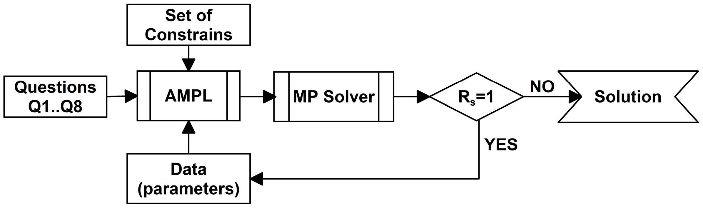
The first approach belongs to the exact methods. Its main purpose was to obtain results that will enable the verification of the approximate methods used for this model and the basis for analysis of the operator using small-sized examples. Its essential feature and important element is coding constraints (1a)–(15) and questions Q1–8 of the model using AMPL. The AMPL model is universal, and it can be solved by many mathematical programming solvers such as: CPLEX, Gurobi, Xpress, Baron, Ilog, and LINDO (commercial solvers), as well as Neos, Gecode, and CBC (open source) [10]. The AMPL model for the EVRPD is included in Appendix A. However, Gurobi is the fastest and most powerful mathematical programming solver available for LP (linear programming), QP (quadratic programming), MILP (mixed integer programming), MIQP (mixed integer programs with quadratic terms in the objective function), and MIQCP (mixed integer programs with quadratic terms in the constraints) problems. Two mathematical programming environments, Gurobi [51] and LINGO [52], were used for the implementation.
Gurobi has an extensive set of algorithms, and its own procedures and functions were used to solve discrete optimization problems. Like other solvers, it uses variants of known methods such as branch-and-bound, cutting planes, etc. Solving the discrete optimization problem using Gurobi was divided into certain steps and blocks. The first step was pre-solving, which aimed to tighten the formulation and reduce the problem size (the procedures and functions used were: Presolve, PrePasses, AggFill, Aggregate, DualReductions, PreSparsify, and ImproveStartTime). The next step was to solve the continuous relaxations (the procedures and functions used were: Method and NodeMethod). At this stage, ignoring integrity occurred, and a bound was given on the optimal integral objective. The next step was to cut off relaxation solutions (the procedures and functions used were: Cuts, CutPasses, CutAggPasses, and GomoryPasses). After which, the branching variable selection took place, which was crucial for limiting the search tree size. Here the VarBranch procedure was applied. In the last step, primal heuristics (Heuristics, MinRelNodes, PumpPasses, RINS, SubMIPNodes, and ZeroObjNodes) were used to find integer-feasible solutions.
LINGO is a comprehensive tool designed to make building and solving linear, non-linear (convex, nonconvex, and global), quadratic, quadratically constrained, second-order cone, semi-definite, stochastic, and integer optimization models faster, easier, and more efficient.
It should be mentioned that more than 2500 companies in over 40 industries turn data into smarter decisions with Gurobi products [51]. By contrast, the number of researchers and educational institutions using this product is difficult to estimate. A schematic diagram of the exact proposed approach is shown in Figure 1.
4.2. Dedicated Genetic Algorithm
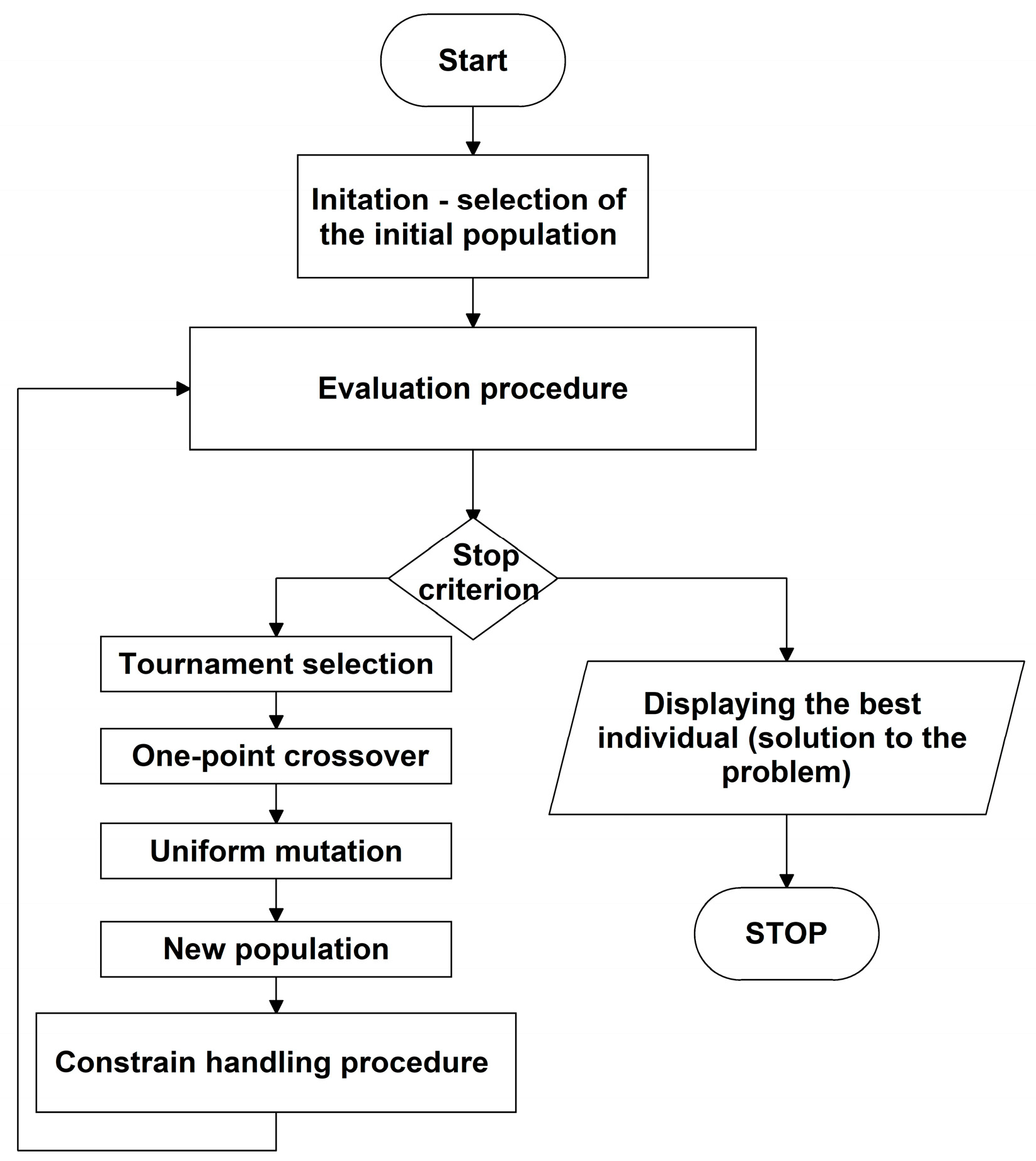
In contrast, the proposed dedicated genetic algorithm (DGA) is metaheuristic and is designed to solve real- and industrial-sized examples of the EVRPD. It is an approximate method like any other metaheuristic. The proposed genetic algorithm (Figure 2) was an alternative to the MP solver.
What distinguishes this algorithm from classical GA is: the dedicated representation of the EVRPD (Section 4.2.1), dedicated selection of the initial population (Section 4.2.2), constraint handling procedure (Section 4.2.3) and an evaluation procedure (Section 4.2.4) which contain elements of pre-solving the problem being solved.
4.2.1. Dedicated Representation of Individuals for the EVRPD
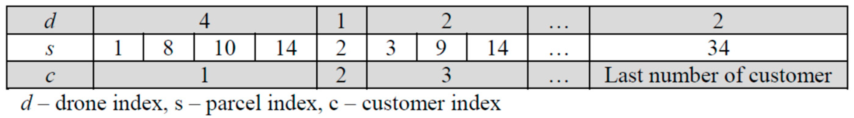
This algorithm used an appropriate representation of individuals for the EVRPD, which, considering the knowledge of the problem, reduced the number of unfulfilled constraints during the operation of the algorithm. Everyone in the population was determined by customer index j∈C which was assigned to a specific drone d∈D. Thus, it was a two-dimensional representation with delivered shipments and parcels s∈S assigned in pairs (j, d). The proposed representation is shown in Figure 3. It should be emphasized that the index s has been included in Figure 3 to better demonstrate the proposed representation. In practice, the pair (j, d) was enough to code an individual.
Using this representation, the number of unfulfilled constraints was reduced. This representation of an individual meant that only the following constraints were not fulfilled: constraint (5)—the drone’s payload; constraint (9)—the drone’s run was executed within the required time; constraint (14)—take-offs were only from the allowed number of MH points. Therefore, in the developed genetic algorithm (Figure 2) for the generation of individuals, corrections were proposed that eliminated individuals who did not fulfill constraints (a)–(c). A detailed description of individual DGA elements is presented in Section 4.2.1 and Section 4.2.4.
4.2.2. Initiation—Selection of the Initial Population
The selection of the initial population was carried out in two steps. In the first step, shipments were grouped into packages. Grouping was completed according to customers. For each package of shipments, a drone was selected to deliver it to the customer. This was an element of pre-solving because before we started solving the problem, we simplified and reduced it. We operated on packages already assigned to customers and drones, which reduced the space of the solutions. In the second step, the constraint handling procedure (Section 4.2.4) was run to check that the drone’s payload was not exceeded. The same procedure was run after the genetic operations and the generation of a new population.
4.2.3. Evaluation Procedure
The evaluation procedure assessed the newly generated population. The basic criterion for evaluation was cost, but the distance was also considered. In the proposed genetic algorithm (DGA), the evaluation procedure consisted of solving the TSP multiple times (through dedicated heuristics) for subsequent MHs. In detail, this procedure worked in two steps:
- Step 1: The traveling salesman problem (TSP) was solved for each MH starting point and each drone. The route was determined in such a way that the cost of delivery was the lowest, and the delivery time was within the set time.
- Step 2: The MH starting points were selected in such a way that the total cost of deliveries was as low as possible and that the number of allowed starting points was not exceeded. This step also ensured that constraint (14) was satisfied.
Step 2 of the evaluation procedure also performed the pre-solving of the modeled problem by eliminating some starting points from the solution space.
4.2.4. Constraint Handling Procedure
The constraint handling procedure for the DGA checks that the drone’s payload was not exceeded. It worked as follows: If the drone’s payload was smaller than the assigned load, the parcels were transferred to another drone for which the allocation would not result in exceeding its payload (the direction of the parcel was considered, i.e., whether it was a delivery or pick up).
If it was not possible to execute the allocation, the largest package of shipments was divided in half, and the procedure was repeated. If there were no more packages to be divided and the allocation could not be determined, and the capacity of the drones was too small in relation to the number of shipments, the algorithm would be stopped. This procedure ensured that both constraints (5) and (9) were satisfied.
4.2.5. Genetic Operators
Traditional genetic operators were used in the DGA—tournament selection, one-point crossover, and mutation. For tournament selection, individuals from the current population were randomly selected into groups of two (tournament size equal to two). The number of groups for the selection must be equal to the size of the population. The selection operator chose one individual from each group (the algorithm worked on a fixed number of individuals in the population). For the individual to be placed in a mating pool, its objective function value must be lower than that of the other individuals in the group. In the next step, mating pairs were randomly selected from the mating pool to undergo a one-point crossover in accordance with the set crossover probability (a constant moderate level of the crossover rate was adopted in this study). In this case, the crossover involved the exchange of fragments between parent individuals at a randomly generated crossover point. The new individuals (two new individuals are produced for each pair of parents) satisfied the problem assumptions. The new individuals were subject to uniform mutation according to the set moderate level of mutation probability. The practical implementation of the mutation operator in the presented problem consisted of the random selection of a parcel and then the random generation of a drone number for the parcel.
The genetic algorithm terminated when it reached the number of iterations set by the program’s user, or an additional stop criterion was defined by the lack of improvement in the quality of the best individual in the population in the next 50 generations.
In this study, the population size was selected empirically with respect to the dimensions of the problem. However, some assumptions were made. The population could not be less than the number of customers (c∈C). However, the number of generations was not less than twice the number of customers. For smaller data instances, these values were greater than these thresholds, and for smaller ones, they were close to them. The remaining values of the parameters of the genetic algorithm were also experimentally determined, inspired by the research described in [53]. Thus, the crossover probability was set at 0.5 and the mutation probability at 0.1.
5. Computational Examples
The computational experiments were carried out in two stages. The first stage concerned the verification of the scope of the decisions supported by the model (constraints (1)–(15) and questions Q1–6). At this stage of the experiments, the model with questions Q7 and Q8 was not tested. For this purpose, computational experiments E01–32 were performed for different data instances. Customer location data were taken from the available benchmarks [54]. For all experiments of this phase, customer location data from the 10.10.1.txt instance were used. The test data had been supplemented with MH points (MH1–3). The remaining values of the model parameters were adopted as in the AMPL model (as shown in Appendix A) as well as the same data in tabular form in Appendix B. Data instances E01–16 differed in the number of trucks, drones, MH points, etc., and questions Q1–6 were under consideration. The cost and method of deliveries were sought. Two approaches were used to implement the models. The first was AMPL with the Gurobi solver (Section 4.1), while the second was the proprietary DGA (Section 4.2). The obtained results of the experiments are presented in Table 4.
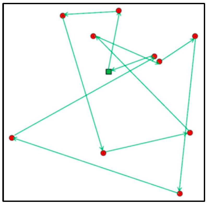
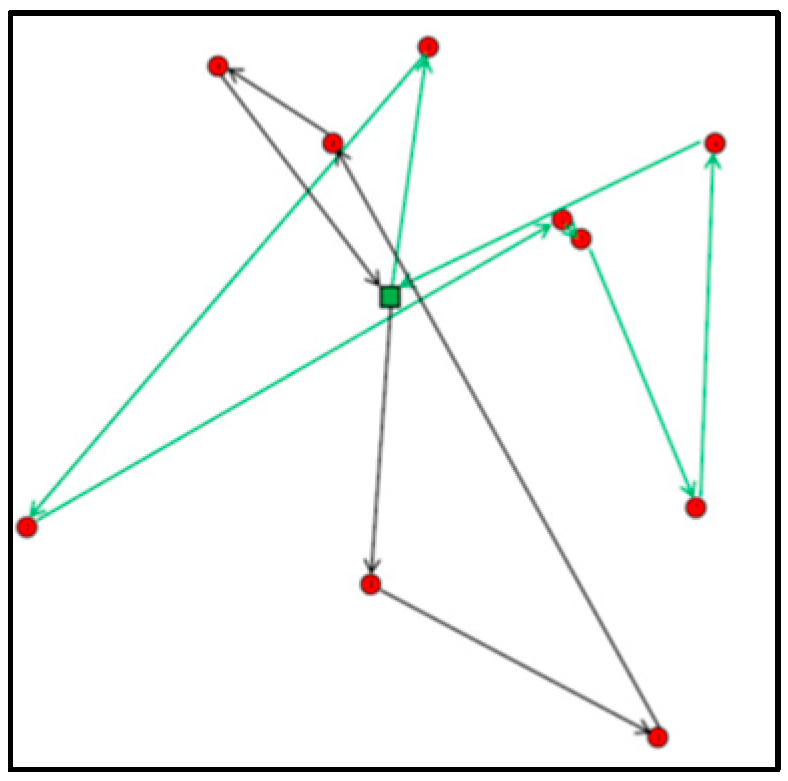
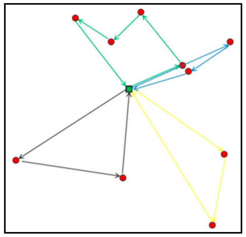
Additionally, they were illustrated for selected data instances as drone routes in Appendix C (see Figure A1, Figure A2, Figure A3, Figure A4, Figure A5 and Figure A6). Due to the typically proactive nature of Q5 and Q6 questions, the obtained answers could be successfully used as input data for the remaining questions. Additionally, for these questions, considering drone routes was irrelevant, and they were not part of the decision for these questions. The obtained results (FC value) differed for Q1 and Q3 (see E01, E03, E05, E09, E13, and E16). These were feasible solutions, and the DGA found better solutions each time. For the remaining experiments, both approaches generated the same FC value. As for the computation time, for these sizes of problems, it was similar for both approaches and ranged from a second to about a minute. An interesting result, in addition to the FC value obtained and the method of deliveries (routes), was information on the number of trucks and drones used (noted in parentheses) and the actual delivery time in relation to the nominal values of the parameters mentioned.
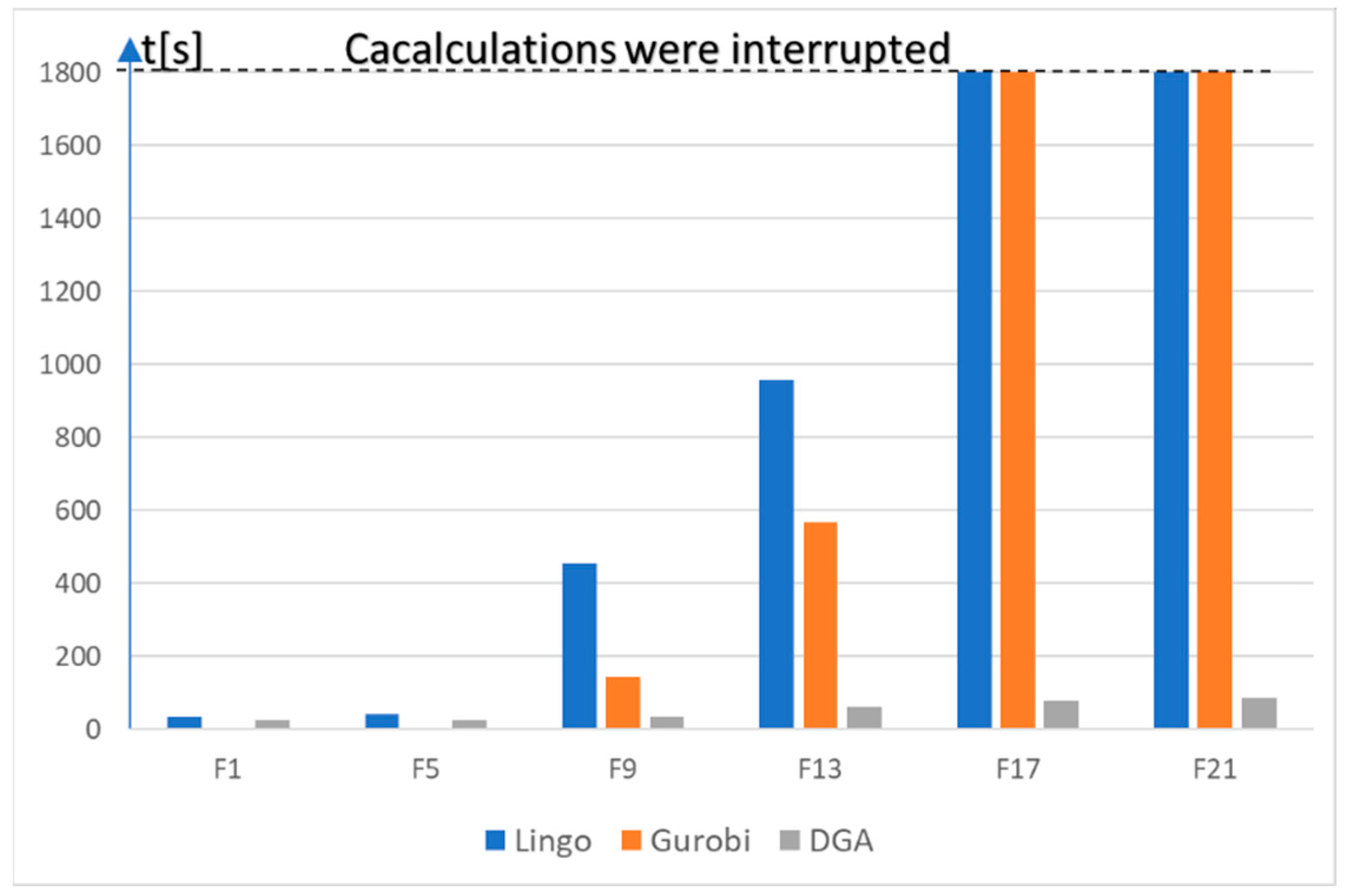
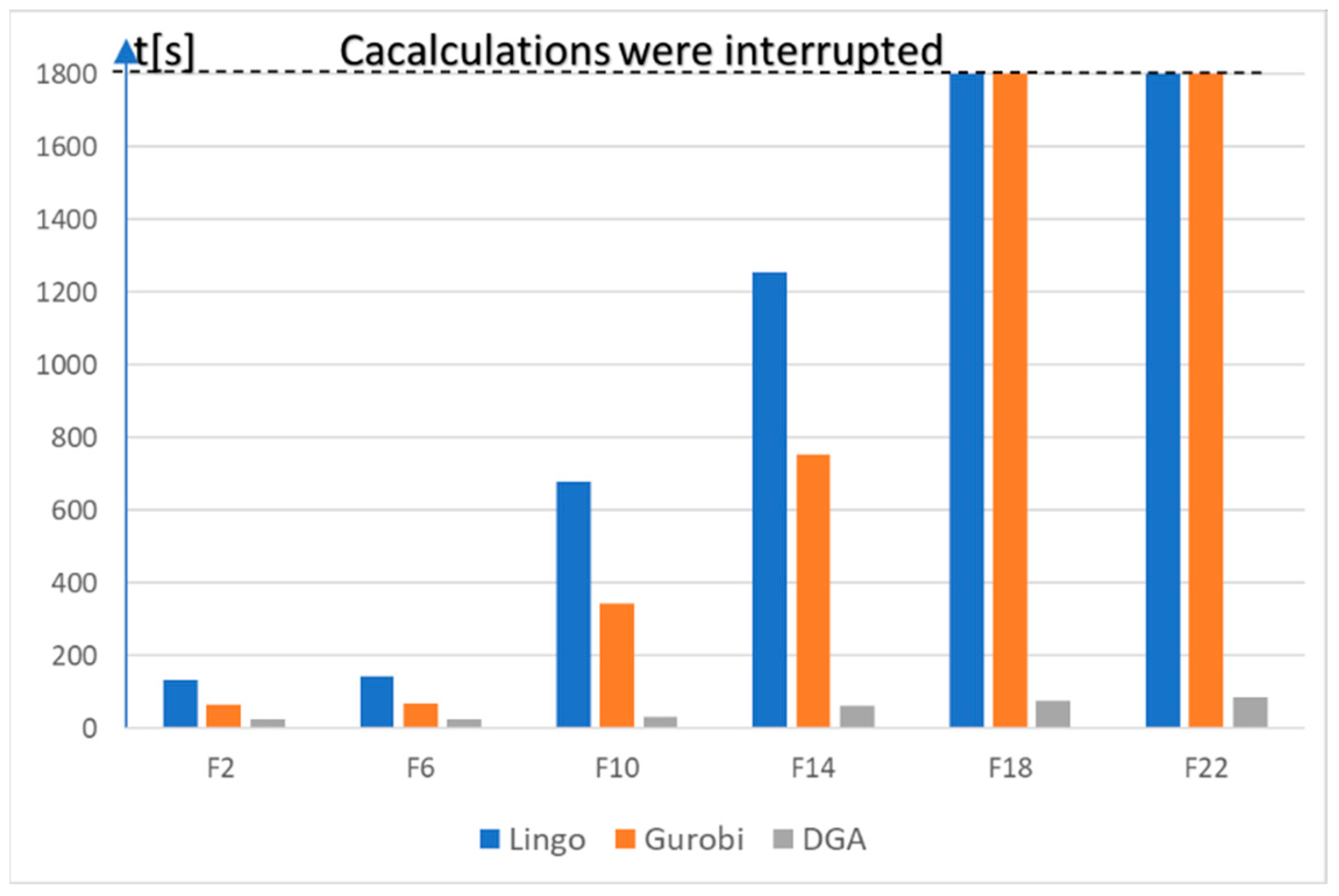
In the second stage, the experiments verified the usefulness of both proposed approaches to model implementation (mathematical programming solvers, Gurobi, LINGO, and the proprietary DGA). Therefore, they were performed on a larger number of data instances, often of larger sizes (10.10.1.txt, 10.10.3.txt, 12.10.1.txt, 20.10.1.txt, 50.10.1.txt, 100.10.1.txt) [54] for questions Q2, Q4, Q5, and Q6. This is because these questions were computationally very demanding (combinatorial optimization). The individual experiments F1–24 differed, e.g., the number of packages and the number of drones. The obtained results are presented in Table 5. After analyzing the results, it could be concluded that the exact approach (AMPL+Gurobi and AMPL+LINGO) works and is acceptable only for small data instances (F1–16). For the remaining data instances, either no solution could be obtained (F21–24) or solutions were obtained after stopping calculations (F17–20) with a worse FC value. Therefore, for larger instances of data, the recommended approach is DGA, which made it possible to obtain a solution in an acceptable time. This was due, on the one hand, to the general properties of this metaheuristic, but also to the adaptation to this problem.
A comparative analysis of the proposed implementation methods was made in terms of computation time. The computation times for the selected data instances were compared and presented in the form of a bar chart. A comparison was made between Q2 and Q4 and is presented in Figure 4 and Figure 5, respectively.
The computational experiments used AMPL, Gurobi 9.1, LINGO 19, proprietary DGA implementation, and a computer with the following parameters: Intel (R) Core (TM) i5-4200M CPU @ 2.50 GHz, 8 GB RAM, Win 64×.
6. Conclusions
The proposed model for the EVRPD could be the basis for building decision support systems for last-mile delivery or urban logistics. It could also be used to answer ad hoc questions related to last-mile delivery and, with minor changes, to other types of vehicles [55,56,57].
In this version, the presented model supported the decisions related to the optimization of routes, the number of drones and vehicles, delivery costs, etc. (Section 3.2).
An important innovation was the flexible structure (a set of constraints and a set of questions that could be easily extended) and great versatility of the presented model, as well as the introduction of the decision variable Rs, causing the proposed model to always have a solution. The introduction of this variable allows you to manage undelivered shipments, e.g., deciding to outsource their deliveries to third parties, short-term rental of additional drones or vehicles, etc.
The method of parameterization of the model and its structure allowed, in subsequent versions, to consider weather conditions, routes in 3D dimension, etc.
This study also proposed two methods of implementing the modeled problem. The first was an exact method and was characterized by high versatility, which resulted from the use of the universal AMPL. This resulted in the possibility of using most of the MP solvers available on the market for the solution. Nevertheless, due to the combinatorial nature of the problem, a second method, DGA, has been proposed.
The presented metaheuristics were adjusted to the EVRPD, e.g., in terms of problem representation, coding, evaluation, and constraint handling procedures. Both procedures used elements of pre-solving the modeled problem, which reduced the space and shortened the time until the solution. All this made it possible to solve much larger problems (up to 20 times) compared with the first method within an acceptable time (Table 5).
Further work will focus on expanding the EVRPD model by adding new questions and new constraints which consider the specificity of drone technology (the range of the drone depending on the weather conditions, cargo delivered, etc.), and road traffic between MHs, etc. Research on appropriate DGA-tuning based on [53] will also be undertaken.
Author Contributions
Conceptualization, P.S. and J.W.; Data curation, J.W.; Formal analysis, P.S.; Software, J.W.; Supervision, P.S.; Validation, M.J.; Visualization, M.J.; Writing—original draft, P.S.; Writing—review & editing, M.J. All authors have read and agreed to the published version of the manuscript.
Funding
This research received no external funding.
Institutional Review Board Statement
Not applicable.
Informed Consent Statement
Not applicable.
Data Availability Statement
Conflicts of Interest
The authors declare no conflict of interest.
Appendix A. AMPL Model for the EVRPD (Files Ready to Use for the Gurobi Solver)
File r.mod
set SH;
set SP;
set SC;
set SS;
set SD;
param VS{SS};
param UA{SS};
param VC{SD};
param RA{SS,SP};
param FA{SP,SP};
param TA{SP,SP};
param MXX;
param ST;
param N_MH;
var Z{SH} >=0, binary;
var X{SH,SD,SP,SP} >=0, binary;
var Y{SH,SD,SP,SP,SS} >=0, binary;
var FC1A;
var FC1B;
var TX;
var R{SS};
minimize fc: FC1A;
subject to C1a: sum{h in SH, d in SD, j in SP, c in SP}
FA[c,j]*X[h,d,c,j]=FC1A;
subject to C1b: sum{h in SH, d in SD, j in SP, c in SP:c<=N_MH} X[h,d,c,j]=FC1B;
subject to C2 {h in SH, d in SD, c in SP}:
sum{j in SP} X[h,d,c,j] = sum{j in SP} X[h,d,j,c];
subject to C3 {h in SH, d in SD, c in SP, j in SP : c> N_MH and j> N_MH
and c<>j}: X[h,d,c,j]<=sum{s in SS} Y[h,d,c,j,s];
subject to C4 {h in SH, d in SD, c in SP, j in SP, s in SS: c<>j}:
Y[h,d,c,j,s]<=X[h,d,c,j];
subject to C5 {h in SH, d in SD, c in SP, j in SP}:
sum{s in SS} VS[s]*Y[h,d,c,j,s]<=VC[d];
subject to C6a {s in SS, j in SP: UA[s]=1 and RA[s,j]=1}:
sum{d in SD, c in SP, h in SH} Y[h,d,c,j,s] = RA[s,j]-R[s];
subject to C6b {s in SS, j in SP: UA[s]=0 and RA[s,j]=1}:
sum{d in SD, c in SP, h in SH} Y[h,d,j,c,s] = RA[s,j]+R[s];
subject to C7 {d in SD}:
sum{h in SH, c in SP, j in SP:c<= N_MH } X[h,d,c,j] <= 1;
subject to C8a {c in SP, s in SS: UA[s]=1}:
sum{j in SP, d in SD, h in SH: c<>j} Y[h,d,j,c,s]-
sum{j in SP, d in SD, h in SH: c<>j} Y[h,d,c,j,s]
=RA[s,c]-R[s];
subject to C8b {c in SP, s in SS: UA[s]=0}:
sum{j in SP, d in SD, h in SH: c<>j} Y[h,d,j,c,s]-
sum{j in SP, d in SD, h in SH: c<>j} Y[h,d,c,j,s]
=-RA[s,c]+R[s];
subject to C9 {d in SD}:
sum{h in SH, c in SP, j in SP} TA[c,j]*X[h,d,c,j]<=TX;
subject to C10a {s in SS :UA[s]=1}:
sum{h in SH, d in SD, j in SP} Y[h,d,h,j,s]=1;
subject to C10b {s in SS :UA[s]=0}:
sum{h in SH, d in SD, j in SP} Y[h,d,j,h,s]=1;
subject to C11 {c in SC}:
sum{h in SH, d in SD, j in SP} X[h,d,j,c+ N_MH]=1;
subject to C12 {h in SH, d in SD, c in SP, j in SP:c<= N_MH and h<>c}:
X[h,d,c,j]=0;
subject to C13 {h in SH}:
Z[h]*ST>=sum{d in SD, c in SP, j in SP} X[h,d,c,j];
subject to C14 :
MXX>=sum{h in SH} Z[h];
FILE r.dat
data;
set SH :=1 2 3 ;
set SP :=1 2 3 4 5 6 7 8 9 10 11 12 13 ;
set SC :=1 2 3 4 5 6 7 8 9 10 ;
set SD :=1 2 3 4 ;
set SS :=1 2 3 4 5 6 7 8 9 10 ;
param VS:= 1 1 2 1 3 1 4 1 5 1 6 1 7 1 8 1 9 1 10 1;
param UA:= 1 1 2 1 3 1 4 1 5 1 6 1 7 1 8 1 9 1 10 1;
param VC:= 1 10 2 10 3 10 4 10;
param TX=50;
param MXX=2;
param N_MH=3;
param ST=1000;
param RA: 1 2 3 4 5 6 7 8 9 10 11 12 13:=
1 0 0 0 1 0 0 0 0 0 0 0 0 0
2 0 0 0 0 1 0 0 0 0 0 0 0 0
3 0 0 0 0 0 1 0 0 0 0 0 0 0
4 0 0 0 0 0 0 1 0 0 0 0 0 0
5 0 0 0 0 0 0 0 1 0 0 0 0 0
6 0 0 0 0 0 0 0 0 1 0 0 0 0
7 0 0 0 0 0 0 0 0 0 1 0 0 0
8 0 0 0 0 0 0 0 0 0 0 1 0 0
9 0 0 0 0 0 0 0 0 0 0 0 1 0
10 0 0 0 0 0 0 0 0 0 0 0 0 1
;
param FA: 1 2 3 4 5 6 7 8 9 10 11 12 13:=
1 0 2 4 3 6 7 5 3 1 5 3 4 3
2 2 0 5 4 5 9 6 5 1 7 4 2 3
3 4 5 0 4 7 3 5 4 5 2 2 7 6
4 3 4 4 0 8 7 2 1 3 4 5 5 3
5 6 5 7 8 0 8 10 8 6 9 4 7 8
6 7 9 3 7 8 0 8 7 8 3 4 10 9
7 5 6 5 2 10 8 0 2 5 5 7 7 4
8 3 5 4 1 8 7 2 0 4 4 5 5 3
9 1 1 5 3 6 8 5 4 0 6 5 2 2
10 5 7 2 4 9 3 5 4 6 0 4 9 7
11 3 4 2 5 4 4 7 5 5 4 0 7 6
12 4 2 7 5 7 10 7 5 2 9 7 0 3
13 3 3 6 3 8 9 4 3 2 7 6 3 0
;
param TA: 1 2 3 4 5 6 7 8 9 10 11 12 13:=
1 0 1 2 1 3 3 2 1 1 3 2 2 1
2 1 0 3 2 2 4 3 2 1 4 2 1 2
3 2 3 0 2 3 2 3 2 2 1 1 4 3
4 1 2 2 0 4 4 1 0 2 2 3 2 1
5 3 2 3 4 0 4 5 4 3 4 2 3 4
6 3 4 2 4 4 0 4 3 4 1 2 5 5
7 2 3 3 1 5 4 0 1 3 2 3 3 2
8 1 2 2 0 4 3 1 0 2 2 2 3 2
9 1 1 2 2 3 4 3 2 0 3 2 1 1
10 3 4 1 2 4 1 2 2 3 0 2 4 4
11 2 2 1 3 2 2 3 2 2 2 0 3 3
12 2 1 4 2 3 5 3 3 1 4 3 0 1
13 1 2 3 1 4 5 2 2 1 4 3 1 0
model r.mod;
data r.dat;
option solver gurobi;
solve;
Appendix B. Data for EVRPD
| k | 1 | 2 | 3 | 4 | 5 | 6 | 7 | 8 | 9 | 10 |
| Vkk | 1 | 1 | 1 | 1 | 1 | 1 | 1 | 1 | 1 | 1 |
| UAk | 1 | 1 | 1 | 1 | 1 | 1 | 1 | 1 | 1 | 1 |
| k | 1 | 2 | 3 | 4 |
| VCd | 10 | 10 | 10 | 10 |
| WAk,o | o | |||||||||||||
| 1 | 2 | 3 | 4 | 5 | 6 | 7 | 8 | 9 | 10 | 11 | 12 | 13 | ||
| k | 1 | 0 | 0 | 0 | 1 | 0 | 0 | 0 | 0 | 0 | 0 | 0 | 0 | 0 |
| 2 | 0 | 0 | 0 | 0 | 1 | 0 | 0 | 0 | 0 | 0 | 0 | 0 | 0 | |
| 3 | 0 | 0 | 0 | 0 | 0 | 1 | 0 | 0 | 0 | 0 | 0 | 0 | 0 | |
| 4 | 0 | 0 | 0 | 0 | 0 | 0 | 1 | 0 | 0 | 0 | 0 | 0 | 0 | |
| 5 | 0 | 0 | 0 | 0 | 0 | 0 | 0 | 1 | 0 | 0 | 0 | 0 | 0 | |
| 6 | 0 | 0 | 0 | 0 | 0 | 0 | 0 | 0 | 1 | 0 | 0 | 0 | 0 | |
| 7 | 0 | 0 | 0 | 0 | 0 | 0 | 0 | 0 | 0 | 1 | 0 | 0 | 0 | |
| 8 | 0 | 0 | 0 | 0 | 0 | 0 | 0 | 0 | 0 | 0 | 1 | 0 | 0 | |
| 9 | 0 | 0 | 0 | 0 | 0 | 0 | 0 | 0 | 0 | 0 | 0 | 1 | 0 | |
| 10 | 0 | 0 | 0 | 0 | 0 | 0 | 0 | 0 | 0 | 0 | 0 | 0 | 1 | |
| FAo,j | j | |||||||||||||
| 1 | 2 | 3 | 4 | 5 | 6 | 7 | 8 | 9 | 10 | 11 | 12 | 13 | ||
| o | 1 | 0 | 2 | 4 | 3 | 6 | 7 | 5 | 3 | 1 | 5 | 3 | 4 | 3 |
| 2 | 2 | 0 | 5 | 4 | 5 | 9 | 6 | 5 | 1 | 7 | 4 | 2 | 3 | |
| 3 | 4 | 5 | 0 | 4 | 7 | 3 | 5 | 4 | 5 | 2 | 2 | 7 | 6 | |
| 4 | 3 | 4 | 4 | 0 | 8 | 7 | 2 | 1 | 3 | 4 | 5 | 5 | 3 | |
| 5 | 6 | 5 | 7 | 8 | 0 | 8 | 10 | 8 | 6 | 9 | 4 | 7 | 8 | |
| 6 | 7 | 9 | 3 | 7 | 8 | 0 | 8 | 7 | 8 | 3 | 4 | 10 | 9 | |
| 7 | 5 | 6 | 5 | 2 | 10 | 8 | 0 | 2 | 5 | 5 | 7 | 7 | 4 | |
| 8 | 3 | 5 | 4 | 1 | 8 | 7 | 2 | 0 | 4 | 4 | 5 | 5 | 3 | |
| 9 | 1 | 1 | 5 | 3 | 6 | 8 | 5 | 4 | 0 | 6 | 5 | 2 | 2 | |
| 10 | 5 | 7 | 2 | 4 | 9 | 3 | 5 | 4 | 6 | 0 | 4 | 9 | 7 | |
| 11 | 3 | 4 | 2 | 5 | 4 | 4 | 7 | 5 | 5 | 4 | 0 | 7 | 6 | |
| 12 | 4 | 2 | 7 | 5 | 7 | 10 | 7 | 5 | 2 | 9 | 7 | 0 | 3 | |
| 13 | 3 | 3 | 6 | 3 | 8 | 9 | 4 | 3 | 2 | 7 | 6 | 3 | 0 | |
| TAo,j | o | |||||||||||||
| 1 | 2 | 3 | 4 | 5 | 6 | 7 | 8 | 9 | 10 | 11 | 12 | 13 | ||
| j | 1 | 0 | 1 | 2 | 1 | 3 | 3 | 2 | 1 | 1 | 3 | 2 | 2 | 1 |
| 2 | 1 | 0 | 3 | 2 | 2 | 4 | 3 | 2 | 1 | 4 | 2 | 1 | 2 | |
| 3 | 2 | 3 | 0 | 2 | 3 | 2 | 3 | 2 | 2 | 1 | 1 | 4 | 3 | |
| 4 | 1 | 2 | 2 | 0 | 4 | 4 | 1 | 0 | 2 | 2 | 3 | 2 | 1 | |
| 5 | 3 | 2 | 3 | 4 | 0 | 4 | 5 | 4 | 3 | 4 | 2 | 3 | 4 | |
| 6 | 3 | 4 | 2 | 4 | 4 | 0 | 4 | 3 | 4 | 1 | 2 | 5 | 5 | |
| 7 | 2 | 3 | 3 | 1 | 5 | 4 | 0 | 1 | 3 | 2 | 3 | 3 | 2 | |
| 8 | 1 | 2 | 2 | 0 | 4 | 3 | 1 | 0 | 2 | 2 | 2 | 3 | 2 | |
| 9 | 1 | 1 | 2 | 2 | 3 | 4 | 3 | 2 | 0 | 3 | 2 | 1 | 1 | |
| 10 | 3 | 4 | 1 | 2 | 4 | 1 | 2 | 2 | 3 | 0 | 2 | 4 | 4 | |
| 11 | 2 | 2 | 1 | 3 | 2 | 2 | 3 | 2 | 2 | 2 | 0 | 3 | 3 | |
| 12 | 2 | 1 | 4 | 2 | 3 | 5 | 3 | 3 | 1 | 4 | 3 | 0 | 1 | |
| 13 | 1 | 2 | 3 | 1 | 4 | 5 | 2 | 2 | 1 | 4 | 3 | 1 | 0 | |
TX=50;
MXX=2;
N_MH=3;
ST=1000;
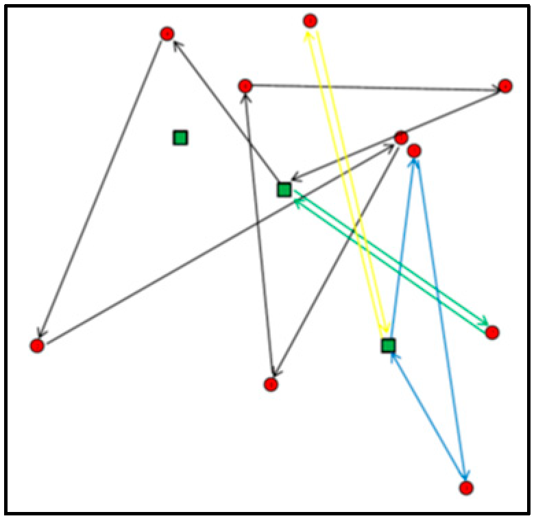
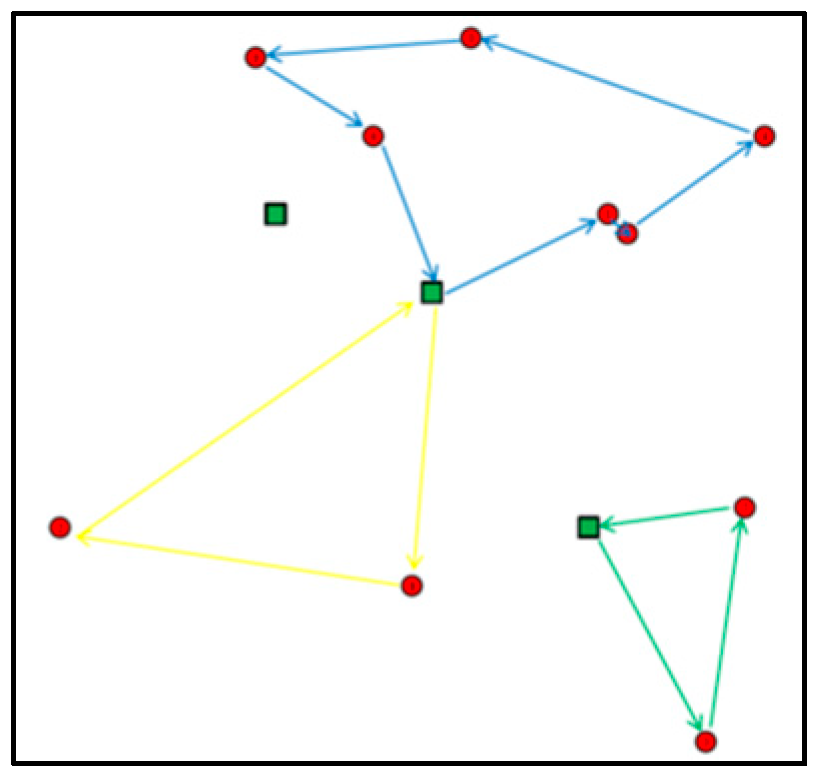
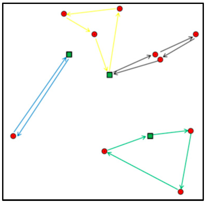
Appendix C. Obtained Routes for Experiments E01, E05, E07, E09, E12 and E16
Figure A1.
Routes for E01.

Figure A2.
Routes for E05.

Figure A3.
Routes for E07.

Figure A4.
Routes for E09.

Figure A5.
Routes for E12.

Figure A6.
Routes for E16.

References
- Aurambout, J.P.; Gkoumas, K.; Ciuffo, B. Last mile delivery by drones: An estimation of viable market potential and access to citizens across European cities. Eur. Transp. Res. Rev. 2019, 11, 30. [Google Scholar] [CrossRef]
- Singireddy, S.R.R.; Daim, T.U. Technology Roadmap: Drone Delivery—Amazon Prime Air. In Infrastructure and Technology Management. Innovation, Technology, and Knowledge Management; Daim, T., Chan, L., Estep, J., Eds.; Springer: Cham, Switzerland, 2018. [Google Scholar] [CrossRef]
- ConnCarProjectReport-1.pdf (berkeley.edu). Available online: https://scet.berkeley.edu/wp-content/uploads/ConnCarProjectReport-1.pdf (accessed on 10 July 2021).
- Merkert, R.; Bushell, J. Managing the drone revolution: A systematic literature review into the current use of airborne drones and future strategic directions for their effective control. J. Air Transp. Manag. 2020, 89, 101929. [Google Scholar] [CrossRef] [PubMed]
- Hern, A. DHL Launches First Commercial Drone ‘Parcelcopter’ Delivery Service. Available online: https://www.theguardian.com/technology/2014/sep/25/german-dhl-launches-first-commercial-drone-delivery-service (accessed on 10 July 2021).
- Drones Are Legit Delivering Pizza Right Now in New Zealand. Available online: https://www.inc.com/will-yakowicz/drone-pizza-delivery-flirtey-dominos.html (accessed on 10 July 2021).
- Amorosi, L.; Puerto, J.; Valverde, C. Coordinating drones with mothership vehicles: The mothership and drone routing problem with graphs. Comput. Oper. Res. 2021, 136, 105445. [Google Scholar] [CrossRef]
- Thibbotuwawa, A.; Bocewicz, G.; Nielsen, P.; Banaszak, Z. Unmanned Aerial Vehicle Routing Problems: A Literature Review. Appl. Sci. 2020, 10, 4504. [Google Scholar] [CrossRef]
- Apt, K.; Wallace, M. Constraint Logic Programming using Eclipse; Cambridge University Press: Cambridge, UK, 2006. [Google Scholar]
- Home AMPL. Available online: https://ampl.com/ (accessed on 10 July 2021).
- Sitek, P.; Wikarek, J.; Bocewicz, G.; Nielsen, I. A decision support model for handling customer orders in business chain. Neurocomputing 2021, 482, 298–309. [Google Scholar] [CrossRef]
- Dell’Amico, M.; Montemanni, R.; Novellani, S. Drone-assisted deliveries: New formulations for the flying sidekick traveling salesman problem. Optim. Lett. 2021, 15, 1617–1648. [Google Scholar] [CrossRef]
- Kim, S.; Moon, I. Traveling salesman problem with a drone station. IEEE Trans. Syst. Man Cybern. Syst. 2018, 49, 42–52. [Google Scholar] [CrossRef]
- Otto, A.; Agatz, N.; Campbell, J.; Golden, B.; Pesch, E. Optimization approaches for civil applications of unmanned aerial vehicles (UAVs) or aerial drones: A survey. Networks 2018, 72, 411–458. [Google Scholar] [CrossRef]
- Park, Y.; Nielsen, P.; Moon, I. Unmanned aerial vehicle set covering problem considering fixed-radius coverage constraint. Comput. Oper. Res. 2020, 119, 104936. [Google Scholar] [CrossRef]
- Phung, M.D.; Quach, C.H.; Dinh, T.H.; Ha, Q. Enhanced discrete particle swarm optimization path planning for UAV vision-based surface inspection. Autom. Constr. 2017, 81, 25–33. [Google Scholar] [CrossRef]
- Sanci, S.; Isler, V. A parallel algorithm for UAV flight route planning on GPU. Int. J. Parallel Program. 2011, 39, 809–837. [Google Scholar] [CrossRef]
- Alidaee, B.; Gao, H.; Wang, H. A note on task assignment of several problems. Comput. Ind. Eng. 2010, 59, 1015–1018. [Google Scholar] [CrossRef]
- Bae, J.; Rathinam, S. Approximation algorithm for a heterogeneous vehicle routing problem. Int. J. Adv. Robot. Syst. 2015, 12. [Google Scholar] [CrossRef]
- Bellingham, J.; Tillerson, M.; Richards, A.; How, J.P. Multi-task allocation and path planning for cooperating UAVs. In Cooperative Control: Models, Applications and Algorithms; Butenko, S., Murphey, R., Pardalos, P.M., Eds.; Springer: Boston, MA, USA, 2003; pp. 23–41. [Google Scholar] [CrossRef]
- Manyam, S.G.; Rathinam, S.; Darbha, S. Computation of lower bounds for a multiple depot, multiple vehicle routing problem with motion constraints. J. Dyn. Syst. Meas. Control 2015, 137, 2378–2383. [Google Scholar] [CrossRef]
- Rathinam, S.; Sengupta, R. Lower and upper bounds for a multiple depot UAV routing problem. In Proceedings of the 45th IEEE Conference on Decision and Control, San Diego, CA, USA, 13–15 December 2006; pp. 5287–5292. [Google Scholar] [CrossRef]
- Sundar, K.; Rathinam, S. Algorithms for heterogeneous, multiple depot, multiple unmanned vehicle path planning problems. J. Intell. Robot. Syst. 2017, 88, 513–526. [Google Scholar] [CrossRef]
- Venkatachalam, S.; Sundar, K.; Rathinam, S. Two-stage stochastic programming model for routing multiple drones with fuel constraints. arXiv 2017, arXiv:1711.04936. [Google Scholar]
- Vilar, R.G.; Shin, H.S. Communication-aware task assignment for UAV cooperation in urban environments. IFAC Proc. 2013, 46, 352–359. [Google Scholar] [CrossRef]
- Gottlieb, Y.; Shima, T. UAVs task and motion planning in the presence of obstacles and prioritized targets. Sensors 2015, 15, 29734–29764. [Google Scholar] [CrossRef]
- Jiang, X.; Zhou, Q.; Ye, Y. Method of task assignment for UAV based on particle swarm optimization in logistics. In Proceedings of the 2017 International Conference on Intelligent Systems, Metaheuristics & Swarm Intelligence, Hong Kong, China, 25–27 March 2017; pp. 113–117. [Google Scholar] [CrossRef]
- Kim, S.J.; Lim, G.J.; Cho, J.; Côté, M.J. Drone-aided healthcare services for patients with chronic diseases in rural areas. J. Intell. Robot. Syst. 2017, 88, 163–180. [Google Scholar] [CrossRef]
- Liu, X.F.; Guan, Z.-W.; Song, Y.-Q.; Chen, D.-S. An optimization model of UAV route planning for road segment surveillance. J. Cent. South Univ. 2014, 21, 2501–2510. [Google Scholar] [CrossRef]
- Phan, D.H.; Suzuki, J. Evolutionary multiobjective optimization for the pickup and delivery problem with time windows and demands. Mob. Netw. Appl. 2016, 21, 175–190. [Google Scholar] [CrossRef]
- Wang, Z.; Sheu, J.B. Vehicle routing problem with drones. Transp. Res. Part B Methodol. 2019, 122, 350–364. [Google Scholar] [CrossRef]
- Murray, C.C.; Chu, A.G. The flying sidekick traveling salesman problem: Optimization of drone-assisted parcel delivery. Transp. Res. Part C Emerg. Technol. 2015, 54, 86–109. [Google Scholar] [CrossRef]
- Murray, C.C.; Raj, R. The multiple flying sidekicks traveling salesman problem: Parcel delivery with multiple drones. Transp. Res. Part C Emerg. Technol. 2020, 110, 368–398. [Google Scholar] [CrossRef]
- Phan, C.; Liu, H.H.T. A cooperative UAV/UGV platform for wildfire detection and fighting. In Proceedings of the 2008 Asia Simulation Conference—7th International Conference on System Simulation and Scientific Computing, Beijing, China, 10–12 October 2008; pp. 494–498. [Google Scholar] [CrossRef]
- Viguria, A.; Maza, I.; Ollero, A. Distributed service-based cooperation in aerial/ground robot teams applied to fire detection and extinguishing missions. Adv. Robot. 2010, 24, 1–23. [Google Scholar] [CrossRef]
- Wu, G.; Pedrycz, W.; Li, H.; Ma, M.; Liu, J. Coordinated planning of heterogeneous Earth observation resources. IEEE Trans. Syst. Man Cybern. Syst. 2016, 46, 109–125. [Google Scholar] [CrossRef]
- Puerto, J.; Valverde, C. Routing for unmanned aerial vehicles: Touring dimensional sets. Eur. J. Oper. Res. 2022, 298, 118–136. [Google Scholar] [CrossRef]
- Rojas, V.; Solano-Charris, E.; Muñoz-Villamizar, A.; Montoya-Torres, J.R. Unmanned aerial vehicles/drones in vehicle routing problems: A literature review. Int. Trans. Oper. Res. 2021, 28, 1626–1657. [Google Scholar] [CrossRef]
- Sujit, P.B.; Sousa, J.; Pereira, F.L. UAV and AUVs coordination for ocean exploration. In Proceedings of the OCEANS 2009-EUROPE, Bremen, Germany, 11–14 May 2009; pp. 1–7. [Google Scholar] [CrossRef]
- Tokekar, P.; Hook, J.V.; Mulla, D.; Isler, V. Sensor planning for a symbiotic UAV and UGV system for precision agriculture. In Proceedings of the 2013 IEEE/RSJ International Conference on Intelligent Robots and Systems, Tokyo, Japan, 3–7 November 2016; Volume 32, pp. 1498–1511. [Google Scholar] [CrossRef]
- Jia, S.; Zhang, L. Modelling unmanned aerial vehicles base station in ground-to-air cooperative networks. IET Commun. 2017, 11, 1187–1194. [Google Scholar] [CrossRef]
- Ladosz, P.; Oh, H.; Chen, W.H. Trajectory planning for communication relay unmanned aerial vehicles in urban dynamic environments. J. Intell. Robot. Syst. 2018, 89, 7–25. [Google Scholar] [CrossRef]
- Oh, H.; Shin, H.S.; Kim, S.; Tsourdos, A.; White, B.A. Cooperative mission and path planning for a team of UAVs. In Handbook of Unmanned Aerial Vehicles; Valavanis, K.P., Vachtsevanos, G.J., Eds.; Springer: Dordrecht, The Netherlands, 2015; pp. 1509–1545. [Google Scholar]
- Sharma, V.; Srinivasan, K.; Kumar, R.; Chao, H.-C.; Hua, K.-L. Efficient cooperative relaying in flying ad hoc networks using fuzzy-bee colony optimization. J. Supercomput. 2017, 73, 3229–3259. [Google Scholar] [CrossRef]
- Dyrkoren, E.; Berg, T. Norwegian work on search and rescue in Barents Sea. In Proceedings of the 33rd International Conference on Offshore Mechanics and Arctic Engineering, Volume 10: Polar and Arctic Science and Technology, San Francisco, CA, USA, 8–13 June 2014. [Google Scholar] [CrossRef]
- Wang, X.; Poikonen, S.; Golden, B. The vehicle routing problem with drones: Several worst-case results. Optim. Lett. 2016, 11, 679–697. [Google Scholar] [CrossRef]
- Poikonen, S.; Wang, X.; Golden, B. The Vehicle Routing Problem with Drones: Extended Models and Connections. Networks 2017, 70, 34–43. [Google Scholar] [CrossRef]
- Ulmer, M.; Thomas, B. Same-Day Delivery with a Heterogeneous Fleet of Drones and Vehicles. Networks 2018, 72, 475–505. [Google Scholar] [CrossRef]
- Dorling, K.; Heinrichs, J.; Messier, G.G.; Magierowski, S. Vehicle Routing Problems for Drone Delivery. IEEE Trans. Syst. Man Cybern. Syst. 2017, 47, 70–85. [Google Scholar] [CrossRef]
- Luo, H.; Liang, Z.; Zhu, M.; Hu, X.; Wang, G. Integrated optimization of unmanned aerial vehicle task allocation and path planning under steady wind. PLoS ONE 2018, 13, e0194690. [Google Scholar] [CrossRef]
- Gurobi—The Fastest Solver. Available online: https://www.gurobi.com/ (accessed on 10 July 2021).
- LINGO and Optimization Modeling. Available online: https://www.lindo.com/index.php/products/lingo-and-optimization-modeling (accessed on 10 July 2021).
- Zhou, Y.; Lee, G.M. A Bi-Objective Medical Relief Shelter Location Problem Considering Coverage Ratios. Int. J. Ind. Eng. Theory Appl. Pract. 2021, 27, 971–988. [Google Scholar] [CrossRef]
- Zenodo—Research. Available online: https://zenodo.org/record/2572764#.YYvxmmDMKUk (accessed on 10 July 2022).
- Wehbi, X.L.; Bektaş, T.; Iris, C. Optimising vehicle and on-foot porter routing in urban logistics. Transp. Res. Part D Transp. Environ. 2022, 109, 103371. [Google Scholar] [CrossRef]
- Caggiani, Y.L.; Colovic, A.; Prencipe, L.P.; Ottomanelli, M. A green logistics solution for last-mile deliveries considering e-vans and e-cargo bikes. Transp. Res. Procedia 2021, 52, 75–82. [Google Scholar] [CrossRef]
- Sacramento, Z.D.; Pisinger, D.; Ropke, S. An adaptive large neighborhood search metaheuristic for the vehicle routing problem with drones. Transp. Res. Part C Emerg. Technol. 2019, 102, 289–315. [Google Scholar] [CrossRef]
Figure 1.
Diagram of model implementation using AMPL and MP solver.

Figure 2.
Block diagram of the proposed dedicated genetic algorithm (DGA).

Figure 3.
The proposed representation of an individual in DGA.

Figure 4.
Comparison of calculation times of Lingo, Gurobi, DGA for Q2.

Figure 5.
Comparison of calculation times of Lingo, Gurobi, DGA for Q4.


Table 1.
(A) Set of questions for the EVRPD. (B) Description of the modeled problems with the use of the EVRPD model.
Table 1.
(A) Set of questions for the EVRPD. (B) Description of the modeled problems with the use of the EVRPD model.
| (A) | ||||
| Symbol | Description | P/R | ||
| Q1 | Is it possible to make deliveries? | P/R | ||
| Q2 | What is the minimum cost of deliveries? | P/R | ||
| Q3 | Is it possible to make deliveries within the given time T? | P/R | ||
| Q4 | What is the minimum cost of deliveries in the given time T? | P/R | ||
| Q5 | What is the minimum number of mobile points (mobile hubs—MHs) required to make deliveries? | P | ||
| Q6 | What is the minimum number of drones needed to make deliveries? | P | ||
| Q7 | Can deliveries be made if the drone dx is damaged? | P | ||
| Q8 | Is it possible to make deliveries if it is not possible to use the mobile point mx? | P | ||
| P/R—proactive/reactive | ||||
| (B) | ||||
| Question | Set of constraints | Problem type | Model type | Decision Variable |
| Q1 | (2)–(8) and (10)–(15) | feasible | CSP | Rs |
| Q2 | (1a) and (2)–(8) and (10)–(15) | optimal | BIP | Xh,d,c,j, Rs |
| Q3 | (2)–(15) | feasible | CSP | Rs |
| Q4 | (1a) and (2)–(15) | optimal | BIP | Xh,d,c,j, Rs |
| Q5 | (2)–(8) and (10)–(15) and min MS | optimal | BIP | Zh |
| Q6 | (1b) and (2)–(8) and (10)–(15) | optimal | BIP | Yh,d,c,j,s |
| Q7 | (2)–(8) and (10)–(15) and VCdi = 0 | feasible | CSP | Rs, Yh,d,c,j,s |
| Q8 | (2)–(8) and (10)–(15) and VKmx = 0 | feasible | CSP | Zh, Xh,d,c,j |
Table 2.
Indices, sets, parameters, and decision variables.
| Symbol | Description |
|---|---|
| Indices and Sets | |
| C | The set of customers |
| S | The set of all items (shipments, parcels) |
| D | The set of all drones |
| H | A set of possible locations for mobile points (mobile hubs—MHs) |
| c, j | Delivery point (customer) index (c, j ∈ C) |
| s | Shipment index (s∈S) |
| d | Drone index (d∈D) |
| h | Mobile point index (h∈K) |
| Parameters | |
| VSs | Parcel volume (volumetric weight) s (s∈S) |
| VCd | Drone’s d payload (d∈D) |
| RAs,c | If parcel k should be delivered to customer o, then RAs,c = 1, otherwise RAs,c = 0 (s∈S, c∈C) |
| FAc,j | Cost of travel between customers c and j (c, j ∈ C ∪ M)—average values include 2D and 3D |
| TAc,j | Transfer time between customers c and j (c, j ∈ C ∪ M)—average values include 2D and 3D |
| TX | Time within which the delivery should be made |
| MS | Maximum number of mobile points (mobile hubs—MHs) |
| ST | A large constant |
| UAs | If parcel s was delivered from the mobile point (MH) to the customer, then UAs = 1; otherwise, UAs = 0 (s∈S). The parameter value determined the delivery direction. |
| Decision variables | |
| Xh,d,c,j | If a drone d traveled from customer c to customer j and took off from MH, h then Xh,d,c,j = 1, otherwise Xh,d,c,j = 0, (h∈H, d∈D, c,j∈C∪M). |
| Yh,d,c,j,s | If a drone d traveled from customer c to customer j and took off from MH, h carrying parcel s, then Yh,d,c,j,s = 1, otherwise Yh,d,c,j,s = 0, (h∈H, d∈D, c, j∈C∪M). |
| Rs | If parcel s could not be delivered, then Rs = 1 otherwise Rs = 0 (s∈S). (The introduction of this decision variable meant that the model will always be solvable.) |
| Zh | If there were take-offs from mobile point h, then Zh = 1; otherwise, Zh = 0. |
Table 3.
Description of the constraints.
| Constraints | Description |
|---|---|
| (1a) | Delivery cost (for Q2 and Q4, it is an objective function (FC1) and is minimized) |
| (1b) | Number of drones used (for Q6, it is an objective function (FC2) and is minimized) |
| (2) | Determined the arrival and departure of the drone at and from the delivery point (customer) |
| (3) | If no items were to be carried on the route, then a drone did not travel that route. |
| (4) | If a drone did not travel along a route, no items were to be carried on that route. |
| (5) | In no route segment could a drone carry more parcels than its payload. |
| (6) | Items were delivered to and from mobile points, h∈H. |
| (7) | Ensured a single run of the drone |
| (8) | Items were picked up or delivered to customers. This constraint prevented sub-tours. |
| (9) | Runs were executed within the required time. |
| (10) | Each drone picked up or delivered parcels from or to a source (MH); the first component of the constraint was responsible for the delivery of parcels to the customer, while the second was responsible for the pick up from the customer. |
| (11) | Ensured the drone was at a point only once (no returns). |
| (12) | Ensured the drone took off and returned to the MH point. (We excluded the possibility that the drone left the parcel with a given customer and another took it to the next customer). |
| (13) | Determined the value of the decision variable Zh. This variable determined mobile point h∈H from the drone take-off point (in this version of the model, we did not introduce capacity limits for trucks, so Zh = 1 determined both the MH point and the truck). |
| (14) | Drone take-offs could not take place from more mobile points h∈H than the number of vehicles (trucks). |
| (15) | Binarity |
Table 4.
The results of the first stage of the experiments for the 10.10.1.txt instance and various Q, N_MH, ST, MI, SC.
Table 4.
The results of the first stage of the experiments for the 10.10.1.txt instance and various Q, N_MH, ST, MI, SC.
| E | Q | N_MH | ST | MI (MO) | SC | TR | AMPL+Gurobi | DGA | |||||
|---|---|---|---|---|---|---|---|---|---|---|---|---|---|
| TX | V | T | FC | TX | T | FC | |||||||
| E01 | Q1 | 1 | 1 | 10 (10) | 1 | 30 | 26 | 1211 | 1 | 56 | 22 | 2 | 48 |
| E02 | Q2 | 1 | 1 | 10 (10) | 1 | 30 | 16 | 1211 | 1 | 34 | 16 | 25 | 34 |
| E03 | Q3 | 1 | 1 | 10 (10) | 1 | 16 | 16 | 1221 | 1 | 42 | 16 | 4 | 35 |
| E04 | Q4 | 1 | 1 | 10 (10) | 1 | 16 | 16 | 1211 | 1 | 34 | 16 | 25 | 34 |
| E05 | Q1 | 1 | 1 | 10 (10) | 4 | 30 | 15 | 4841 | 2 | 55 | 18 | 1 | 51 |
| E06 | Q2 | 1 | 1 | 10 (10) | 4 | 30 | 16 | 4841 | 2 | 34 | 16 | 24 | 34 |
| E07 | Q3 | 1 | 1 | 10 (10) | 4 | 10 | 7 | 4841 | 15 | 52 | 7 | 3 | 52 |
| E08 | Q4 | 1 | 1 | 10 (10) | 4 | 10 | 9 | 4841 | 35 | 40 | 9 | 25 | 40 |
| E09 | Q1 | 3 | 2 | 10 (10) | 4 | 30 | 19 | 17,427 | 3 | 75 | 18 | 4 | 66 |
| E10 | Q2 | 3 | 2 | 10 (10) | 4 | 30 | 15 | 17,427 | 3 | 33 | 15 | 25 | 33 |
| E11 | Q3 | 3 | 2 | 10 (10) | 4 | 10 | 6 | 17,427 | 67 | 41 | 6 | 8 | 41 |
| E12 | Q4 | 3 | 2 | 10 (10) | 4 | 10 | 7 | 17,427 | 85 | 37 | 7 | 25 | 37 |
| E13 | Q1 | 3 | 3 | 10 (10) | 4 | 30 | 18 | 17,427 | 2 | 42 | 15 | 10 | 38 |
| E14 | Q2 | 3 | 3 | 10 (10) | 4 | 30 | 15 | 17,427 | 7 | 33 | 15 | 25 | 33 |
| E15 | Q3 | 3 | 3 | 10 (10) | 4 | 8 | 7 | 17,427 | 8 | 52 | 5 | 12 | 50 |
| E16 | Q4 | 3 | 3 | 10 (10) | 4 | 8 | 5 | 17,427 | 12 | 40 | 5 | 25 | 40 |
| E17 | Q5 | 1 | 1 | 10 (10) | 1 | 30 | --- | 1211 | 2 | 1 | --- | 2 | 1 |
| E18 | Q6 | 1 | 1 | 10 (10) | 1 | 30 | --- | 1211 | 2 | 1 | --- | 2 | 1 |
| E19 | Q5 | 1 | 1 | 10 (10) | 1 | 16 | --- | 1211 | 2 | 1 | --- | 2 | 1 |
| E20 | Q6 | 1 | 1 | 10 (10) | 1 | 16 | --- | 1211 | 2 | 1 | --- | 2 | 1 |
| E21 | Q5 | 1 | 1 | 10 (10) | 4 | 30 | --- | 4841 | 2 | 1 | --- | 2 | 1 |
| E22 | Q6 | 1 | 1 | 10 (10) | 4 | 30 | --- | 4841 | 2 | 1 | --- | 2 | 1 |
| E23 | Q5 | 1 | 1 | 10 (10) | 4 | 16 | --- | 4841 | 4 | 1 | --- | 4 | 1 |
| E24 | Q6 | 1 | 1 | 10 (10) | 4 | 16 | --- | 4841 | 34 | 2 | --- | 27 | 2 |
| E25 | Q5 | 3 | 2 | 10 (10) | 4 | 30 | --- | 17,427 | 3 | 1 | --- | 3 | 1 |
| E26 | Q6 | 3 | 2 | 10 (10) | 4 | 30 | --- | 17,427 | 4 | 1 | --- | 4 | 1 |
| E27 | Q5 | 3 | 2 | 10 (10) | 4 | 30 | --- | 17,427 | 48 | 2 | --- | 23 | 2 |
| E28 | Q6 | 3 | 2 | 10 (10) | 4 | 30 | --- | 17,427 | 92 | 3 | --- | 25 | 3 |
| E29 | Q5 | 3 | 3 | 10 (10) | 4 | 30 | --- | 17,427 | 3 | 1 | --- | 3 | 1 |
| E30 | Q6 | 3 | 3 | 10 (10) | 4 | 30 | --- | 17,427 | 1 | 1 | --- | 1 | 1 |
| E31 | Q5 | 3 | 3 | 10 (10) | 4 | 30 | --- | 17,427 | 34 | 2 | --- | 24 | 2 |
| E32 | Q6 | 3 | 3 | 10 (10) | 4 | 30 | --- | 17,427 | 67 | 4 | --- | 28 | 4 |
E—index of the experiment, N_MH—number of mobile points (MHs), ST—number of trucks, T—computation time in seconds, MO—number of recipients (customers), MI—number of shipments (parcels), SC—number of drones, FC—for Q1–4 delivery cost, for Q5 minimum number of mobile points, and for Q6 minimum number of drones, TR—acceptable delivery time, TX—delivery time, V—number of decision variables.
Table 5.
The results of the second stage of the experiments for the various F, Q, ST, MI, SC.
| F (Instance) | Q | MI (MO) | SC | TR | AMPL+Gurobi | AMPL+LINGO | DGA | ||||||
|---|---|---|---|---|---|---|---|---|---|---|---|---|---|
| V | TX | T | FC | T | FC | TX | T | FC | |||||
| F1 (10.10.1.txt) | Q2 | 10 (10) | 4 | 30 | 17,427 | 15 | 3 | 33 | 34 | 33 | 15 | 25 | 33 |
| F2 (10.10.1.txt) | Q4 | 10 (10) | 4 | 8 | 17,427 | 7 | 67 | 37 | 134 | 37 | 7 | 25 | 37 |
| F3 (10.10.1.txt) | Q5 | 10 (10) | 4 | 8 | 17,427 | --- | 4 | 1 | 35 | 1 | --- | 8 | 1 |
| F4 (10.10.1.txt) | Q6 | 10 (10) | 4 | 8 | 17,427 | --- | 54 | 1 | 145 | 1 | --- | 14 | 1 |
| F5 (10.10.3.txt) | Q2 | 10 (10) | 4 | 30 | 17,427 | 14 | 6 | 29 | 41 | 29 | 14 | 24 | 29 |
| F6 (10.10.3.txt) | Q4 | 10 (10) | 4 | 10 | 17,427 | 7 | 68 | 36 | 145 | 36 | 7 | 25 | 36 |
| F7 (10.10.3.txt) | Q5 | 10 (10) | 4 | 10 | 17,427 | --- | 6 | 1 | 45 | 1 | --- | 10 | 1 |
| F8 (10.10.3.txt) | Q6 | 10 (10) | 4 | 10 | 17,427 | --- | 3 | 1 | 189 | 1 | --- | 13 | 1 |
| F9 (12.10.1.txt) | Q2 | 12 (12) | 4 | 30 | 28,395 | 16 | 145 | 32 | 456 | 32 | 16 | 34 | 32 |
| F10 (12.10.1.txt) | Q4 | 12 (12) | 4 | 10 | 28,395 | 10 | 345 | 35 | 678 | 35 | 10 | 33 | 35 |
| F11 (12.10.1.txt) | Q5 | 12 (12) | 4 | 10 | 28,395 | --- | 67 | 2 | 189 | 2 | --- | 23 | 2 |
| F12 (12.10.1.txt) | Q6 | 12 (12) | 4 | 10 | 28,395 | --- | 345 | 2 | 867 | 2 | --- | 34 | 2 |
| F13 (20.10.1.txt) | Q2 | 20 (20) | 4 | 30 | 116,424 | 18 | 567 | 67 | 956 | 67 | 18 | 61 | 67 |
| F14 (20.10.1.txt) | Q4 | 20 (20) | 4 | 12 | 116,424 | 10 | 754 | 82 | 1256 | 82 | 10 | 62 | 82 |
| F15 (20.10.1.txt) | Q5 | 20 (20) | 4 | 12 | 116,424 | --- | 134 | 2 | 565 | 2 | --- | 55 | 2 |
| F16 (20.10.1.txt) | Q6 | 20 (20) | 4 | 12 | 116,424 | --- | 534 | 3 | 987 | 3 | --- | 57 | 3 |
| F17 (50.10.1.txt) | Q2 | 50 (50) | 4 | 30 | 1,727,485 | 28 | 1800 * | 132 | 1800 * | NFSF | 26 | 78 | 128 |
| F18 (50.10.1.txt) | Q4 | 50 (50) | 4 | 25 | 1,727,485 | 24 | 1800 * | 156 | 1800 * | NFSF | 24 | 76 | 141 |
| F19 (50.10.1.txt) | Q5 | 50 (50) | 4 | 25 | 1,727,485 | --- | 1800 * | 2 | 1800 * | NFSF | --- | 77 | 2 |
| F20 (50.10.1.txt) | Q6 | 50 (50) | 4 | 25 | 1,727,485 | --- | 1800 * | 3 | 1800 * | NFSF | --- | 79 | 3 |
| F21 (100.10.1.txt) | Q2 | 100 (100) | 6 | 35 | 19,318,893 | - | 1800 * | NFSF | 1800 * | NFSF | 34 | 87 | 194 |
| F22 (100.10.1.txt) | Q4 | 100 (100) | 6 | 30 | 19,318,893 | - | 1800 * | NFSF | 1800 * | NFSF | 28 | 89 | 210 |
| F23 (100.10.1.txt) | Q5 | 100 (100) | 6 | 30 | 19,318,893 | --- | 1800 * | NFSF | 1800 * | NFSF | --- | 86 | 1 |
| F24 (100.10.1.txt) | Q6 | 100 (100) | 6 | 30 | 19,318,893 | --- | 1800 * | NFSF | 1800 * | NFSF | --- | 85 | 2 |
F—index of the experiment (file of data instance), T—computation time in seconds, MO—number of recipients (customers), MI—number of shipments (parcels), SC—number of drones, FC—for Q1–4 delivery cost, for Q5 minimum number of mobile points, and for Q6 minimum number of drones, TR—acceptable delivery time, TX—delivery time, V—number of decision variables, * calculations were interrupted (here after 1800s).
Publisher’s Note: MDPI stays neutral with regard to jurisdictional claims in published maps and institutional affiliations. |
© 2022 by the authors. Licensee MDPI, Basel, Switzerland. This article is an open access article distributed under the terms and conditions of the Creative Commons Attribution (CC BY) license (https://creativecommons.org/licenses/by/4.0/).
Share and Cite
MDPI and ACS Style
Sitek, P.; Wikarek, J.; Jagodziński, M. A Proactive Approach to Extended Vehicle Routing Problem with Drones (EVRPD). Appl. Sci. 2022, 12, 8255. https://doi.org/10.3390/app12168255
AMA Style
Sitek P, Wikarek J, Jagodziński M. A Proactive Approach to Extended Vehicle Routing Problem with Drones (EVRPD). Applied Sciences. 2022; 12(16):8255. https://doi.org/10.3390/app12168255
Chicago/Turabian StyleSitek, Paweł, Jarosław Wikarek, and Mieczysław Jagodziński. 2022. "A Proactive Approach to Extended Vehicle Routing Problem with Drones (EVRPD)" Applied Sciences 12, no. 16: 8255. https://doi.org/10.3390/app12168255
Note that from the first issue of 2016, this journal uses article numbers instead of page numbers. See further details here.