
Error-Bounded Learned Scientific Data Compression with Preservation of Derived Quantities
by
 , ,
, ,
Jaemoon Lee
1,* ,
,
Qian Gong
2,
Jong Choi
2,
Tania Banerjee
1,
Scott Klasky
2,
Sanjay Ranka
1 and 
Anand Rangarajan
1 1
Department of Computer & Information Science & Engineering, University of Florida, Gainesville, FL 32611, USA
2
Oak Ridge National Laboratory, Oak Ridge, TN 37830, USA
*
Author to whom correspondence should be addressed.
Appl. Sci. 2022, 12(13), 6718; https://doi.org/10.3390/app12136718
Submission received: 7 June 2022
/
Revised: 24 June 2022
/
Accepted: 29 June 2022
/
Published: 2 July 2022
(This article belongs to the Special Issue Artificial Intelligence and Data Engineering in Engineering Applications)
Abstract
:Scientific applications continue to grow and produce extremely large amounts of data, which require efficient compression algorithms for long-term storage. Compression errors in scientific applications can have a deleterious impact on downstream processing. Thus, it is crucial to preserve all the “known” Quantities of Interest (QoI) during compression. To address this issue, most existing approaches guarantee the reconstruction error of the original data or primary data (PD), but cannot directly control the problem of preserving the QoI. In this work, we propose a physics-informed compression technique that is composed of two parts: (i) reduction of the PD with bounded errors and (ii) preservation of the QoI. In the first step, we combine tensor decompositions, autoencoders, product quantizers, and error-bounded lossy compressors to bound the reconstruction error at high levels of compression. In the second step, we use constraint satisfaction post-processing followed by quantization to preserve the QoI. To illustrate the challenges of reducing the reconstruction errors of the PD and QoI, we focus on simulation data generated by a large-scale fusion code, XGC, which can produce tens of petabytes in a single day. The results show that our approach can achieve a high compression amount while accurately preserving the QoI within scientifically acceptable bounds.
1. Introduction
As high-performance computing (HPC) enters the exascale era, scientific simulations are becoming capable of predicting physics phenomena with high accuracy, while generating extremely large volumes of data at high velocity. The increase in data volumes is rapidly outpacing the growth of storage and I/O capacities. For example, climate simulations [1] can generate 260 every 16 s when running large ensembles of high-fidelity 1 km × 1 km simulations of 15 years of climate. This necessitates the development of data compression algorithms for scientific applications that are reliable and can achieve a large reduction ratio. There have been successful approaches for traditional image and video compression [2], but they are not directly applicable to scientific data compression because of scientific post-processing requirements, which markedly differ from visual perception. Unlike image and video processing, where the dimensionality of data is two or three, scientific datasets are typically high-dimensional tensors and have underlying spatial and temporal structure.
Compressing scientific data is challenging because we need a significant reduction of the Primary Data (PD) with a guaranteed error bound, and we need to preserve the downstream Quantities Of Interest (QoI) as accurately as possible. The necessity of guaranteed error bounds of scientific data is due to the need for high accuracy after compression. For example, in turbulence simulations, the paths of turbulence can be estimated by properties such as latitude, longitude, pressure, and so on, which should be preserved to high fidelity during data reduction. This has to be achieved while ensuring that compression algorithms continue to cater to high-performance computing standards to reduce the time spent storing and retrieving the data. The mathematical relationships between the point-wise errors of PD and the errors of QoI are central to scientific data compression and create unique challenges for the reduction community. For this reason, we focus on simultaneously achieving lossy data compression while preserving the QoI to within specific error tolerances.
Data reduction for scientific applications has been extensively studied. Error-bounded lossy compression techniques are considered to be one of the most successful for these applications. Compared to lossless compressors [3,4] that achieve limited compression [5]), error-bounded lossy compressors can significantly reduce the data and, moreover, achieve high fidelity of the reconstructed data according to the user’s required data distortion bounds. The most well-known and state-of-the-art error-bounded lossy compressors in the literature are based on prediction (SZ [6,7,8]), block transform (ZFP [9]), and multilevel decomposition (MGARD [10,11,12]). SZ is designed based on data prediction models. It first performs a preprocessing step such as linearization of multi-dimensional data and predicts each data point based on its neighboring values using a Lorenzo predictor [13]. ZFP is based on orthogonal block transforms and embedded coding. It breaks the data into a set of blocks (4 × 4 × 4 for 3D data) and then applies an orthogonal block transformation to decorrelate the data. The generated coefficients are encoded to produce compressed data. Most error-bounded lossy compression algorithms such as SZ [6,7,8] and ZFP [9] just focus on preserving point-wise values and provide guaranteed error control on the primary data. However, this does not ensure QoI preservation. Derived quantities are critical to accurate post-analysis. Inconsistent moments and energy in XGC applications that simulate gyrokinetic particle motion, for example, cause totally different fusion simulation analysis. MGARD [10,11,12] is currently the leading error-controlled lossy compression technique with QoI preservation. MGARD can bound the errors of linear QoI by using a non-uniform multilevel subgrid algorithm and providing a mathematical error analysis. Despite this, MGARD cannot currently control the reconstruction errors of non-linear or complex QoI that are often necessary for scientific discovery.
In the machine learning (ML) community, there have been many approaches that successfully leverage deep learning for image compression [14,15,16]. The AutoEncoder (AE) technique is a standard deep learning model for data compression. It has an encoder–decoder architecture and is trained to minimize the point-wise error between the PD and the output of the decoder. While numerous AE variations have been developed, the application of ML techniques to scientific datasets is in its infancy. A fully connected AE has been studied for scientific data compression [17]. The network consists of seven fully connected layers: three layers for an encoder and decoder and a bottleneck layer. The model is, however, applied only on small-scale 1D scientific data. For a specific scientific application, a convolutional AE is developed to compress turbulent flow simulation data [18]. The model includes skip connections with residual block structure [19] to reduce the amount of information in both the encoder and the decoder. This enables the network to effectively learn the complex turbulent flow features. However, these approaches do not guarantee the error of reconstructed data.
There have been approaches that improve the efficiency of ML models by training under constraints. Although they are not studied for data reduction, these are closely related to QoI preservation, since QoI preservation can be treated as constraint satisfaction. Physics-informed neural networks [20] have recently received a lot of attention. Many physics simulations require powerful computational resources and are quite expensive to execute. Physics-informed neural networks are investigated to predict simulation results, and therefore can simplify and reduce the cost of entire simulations. Using the fact that many fields of science have closed-form constraints, these are enforced by incorporating the equations into the architecture of neural networks. Therefore, the approaches are limited to specific physics systems such as Reynolds-averaged Navier–Stokes equations [21,22] and advection equations [23,24]. The merits of the models have been demonstrated in solving a number of forward and inverse problems governed by partial differential equations. There are approaches for incorporating QoI using constrained optimization [25,26] that are closely related to our work. While augmented Lagrangians have been used to incorporate physical constraints into neural networks [27,28], some methods merely use soft penalties which violate QoI error tolerances [29,30]. These simulation approaches have not yet been used for compression, which is the focus of our present work.
In this paper, we propose a novel, hybrid, algorithmic framework to address these issues. We combine tensor decompositions, ML autoencoders, error-bounded lossy compressors, constrained optimization, and product quantization to achieve high compression ratios and fidelity of both the PD and the QoI. The approach is general and broadly applicable to any tensor dataset with moment-based constraint QoI preservation (and error-bounded reconstruction). We focus our attention on a large-scale fusion code—XGC [31], which produces petabytes of five-dimensional data in a day. The key data structures for the target applications are arranged in the form of tensors on a structured, irregular, or hybrid grid. Our methods allow suitable trade-offs between the accuracy and compression ratio for such applications, and comprise the following techniques:
- Transformation: We perform tensor decompositions as a preprocessing step to project the tensors within coherent segments into a more suitable space for reduction. We obtain core tensors (or coefficients) and bases. The tensor basis functions are similar to wavelets and/or local spatial frequencies, and are therefore good at expressing the correlations among the tensors.
- Autoencoder-based compression: AEs are trained on the transformed tensor coefficient space. Since tensor basis functions can take care of spatial correlation, AEs encode and decode tensor basis coefficients. We use AEs to obtain the encoded coefficients using standard loss measures and employ a quantization scheme to store the encoded coefficients.
- Error guarantees on PD: Error guarantees in the form of bounded reconstruction error are achieved by selectively applying error-bounded compressors on the residuals. (The residual is the difference between the reconstructed data of the AE and the PD). The residuals are processed with error-bounded lossy compressors to guarantee bounds on the overall PD error.
- QoI satisfaction: Preservation of QoI is addressed using constraint satisfaction on the reconstructed PD. After residual post-processing, we perform constrained optimization while minimizing the changes to the PD reconstruction. The parameters produced as a result of the QoI satisfaction step are quantized and stored with the encoded coefficients and residuals.
Our experimental results show that our framework can achieve high compression ratios when the sizes of the latent space and the quantization dictionary are controlled. Additionally, we show that selective residual post-processing prevents significant distortion of data even at high compression ratios. Furthermore, the constraint satisfaction step can directly manage QoI preservation with tolerable errors (up to two to three orders of magnitude in compression ratios). We compare our framework to MGARD, which is currently the leading error-bounded lossy compressor with QoI preservation, and show that our approach can achieve a significantly better fidelity of PD and QoI.
2. XGC Application
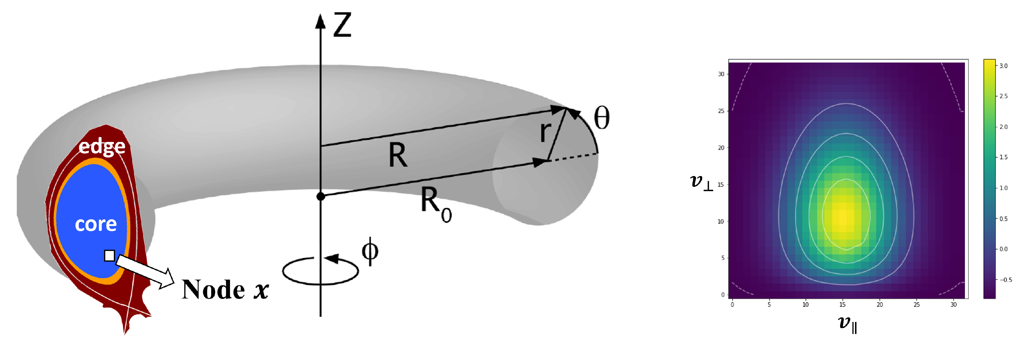
XGC [31,32] is one of the most important first principles fusion codes used to understand the physics in the edge of a fusion experiment, and is part of the DOE Exascale Computing Program. XGC uses a Particle-In-Cell (PIC) technique and evolves a massively large number of particles based on a five-dimensional gyrokinetic equation of motion, three in physical space and two in the velocity space. In XGC, particles are moved according to the physics equations in a time-stepping manner, and then regularly summarized to a discretized 3D space by planes and meshes for solving electric and magnetic field equations. One of the large datasets gathered in the mesh is a particle distribution function, known as a velocity histogram, called F-data (Figure 1).
XGC scientists typically reduce the trillions of particles to build F-data and examine them at every timestep. The size of F-data ranges from hundreds of GB to tens of TBs, depending on the simulation scale. To study the next-generation fusion devices, such as ITER and DEMO, data compression of F-data is necessary for multiple purposes, such as saving memory/disk spaces and analysis speed-up. However, XGC scientists are eager to ensure that various physics properties derived from the distribution, such as mass, canonical angular momentum, and energy, are conserved. Therefore, reducing compression error is needed for this XGC dataset.
More specifically, for F-data compression, XGC scientists are concerned with QoI preservation as well as compression errors. We investigate six physics quantities specified by XGC scientists. The QoI we consider are density n, parallel flow , perpendicular temperature , parallel temperature , flux surface averaged density , and flux surface averaged temperature . In the XGC dataset, each mesh node x has a 2D velocity histogram . The density n and parallel flow are computed by integrating with volume weights and with the parallel velocity, respectively:
where t represents the timestep, is the volume of the mesh node, and is the parallel velocity. and are the integrals of perpendicular and parallel kinetic energy, ,
where m is the mass of atomic particles corresponding to and is the perpendicular velocity. The flux surface averaged density and flux surface averaged temperature are computed by averaging the density and temperature over a thin volume between toroidal magnetic flux surface contours. For simplicity, we omit the detailed equations for the flux surface averaged quantities [33]. Except for density, these QoI are non-linear on and are obtained via post-analysis of the data. In summary, the QoI described here result in four derived quantities (density, parallel flow, perpendicular, and parallel temperatures) which can be used in a constraint satisfaction procedure connecting the primary data () and the QoI. This is precisely the route taken in this paper.
3. The Compression Framework
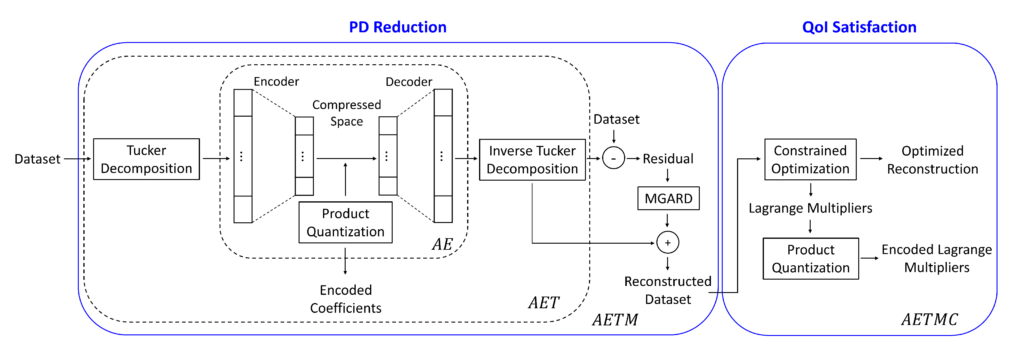
A high-level description of our reduction/compression pipeline is described in Figure 2. The framework mainly comprises two pipelines—Primary Data (PD) reduction and Quantities of Interest (QoI) satisfaction. For PD reduction, we combine Tucker decomposition, an autoencoder (AE), and a product quantizer (PQ) for effective global compression. An error-bounded lossy compressor is used for residual post-processing after global learning to provide the guaranteed error bound on PD. For QoI satisfaction, we perform local constrained optimization on the reconstructed data from the PD reduction pipeline. This step enables us to directly control QoI preservation. We use another product quantizer to encode the Lagrange multipliers produced by this step. Each of these pipelines is now described in detail in the remainder of this section.
3.1. Reduction of the Primary Data
Basis functions can span the spectrum from simple principal/independent component analysis (PCA/ICA) to overcomplete dictionaries. Here, we use the Tucker decomposition [34] to obtain a simple factorization. Each tensor is thereby converted into a set of coefficients, and subsequently, we use an ML autoencoder (AE) with the mean squared error (MSE) measure on the converted Tucker coefficients. The output of the decoder is projected back into the original tensor space to produce a reconstruction. The residual of the reconstruction is then analyzed using an error-bounded lossy compressor to ensure that the PD are within prespecified error bounds. In our approach, we process residuals using MGARD. Note that to get an actual codec, we have to quantize the latent space coefficients in the AE. We use PQ to obtain a codec, with the result being a set of integers for each tensor. Varying the latent space cardinality of the AE yields different compression ratios.
3.1.1. Data Transformation
The Tucker decomposition [34] is widely used in data reduction by considering a subset of coefficients that carry most of the information in the dataset and eliminate lower-rank coefficients, which typically has no adverse effect on tensor reconstruction. The original Tucker decomposition can be viewed as a higher-order singular-value decomposition (HOSVD), and we do not consider more complex variants such as HOOI [35] in this paper. It decomposes a tensor T of order N into a core tensor with the same order while generating N orthonormal bases. If we consider a dataset as a tensor of order 3, its Tucker decomposition is , where is the core tensor which, as a lower rank approximation of T, gives a representation basis for it. Unitary or factor matrices contain basis vectors that help project T into the basis space .
3.1.2. The Autoencoder
An autoencoder is a neural network that is trained to reproduce the input at its output while going through a bottleneck. Internally, it has hidden layers and a final bottleneck hidden layer h that describes a code used to represent the input. The network may be viewed as consisting of two parts: an encoder function and a decoder that produces a reconstruction . If an autoencoder succeeds in simply learning to set everywhere, then it is not especially useful. Instead, autoencoders are designed to be unable to learn to copy perfectly. Usually, they are restricted in ways that allow them to copy only approximately. The model is forced to prioritize which aspects of the input should be copied, and therefore it often learns useful properties of the data.
We obtain the encoded coefficients (the latent space) using standard loss measures in the AE. Consequently, the PD errors are minimized by the AE while learning a good codec. Error guarantees in the form of bounded reconstruction error (at a given level of reduction) on the PD will be achieved by applying error-bounded lossy compressors to the residuals. The loss function of the AE network compares the coefficients of the Tucker decomposition with the reconstruction from the bottleneck latent space:
where X is the input Tucker coefficients and is the reconstructed coefficients.
We use an AE which constrains the number of nodes present in the hidden layers of the network, limiting the amount of information that can flow through the network. By penalizing the network according to the reconstruction error, our model can learn the most important attributes of the input data and how to best reconstruct the original input from an encoded state. Ideally, this encoding will learn and describe latent attributes of the input data. Therefore, the bottleneck layer contains the data compression.
3.1.3. Quantization of the Latent Space
Merely obtaining a latent space is not sufficient to obtain good compression. Entropy encoding of the latent space—also known as quantization—is required to efficiently store the bottleneck layer coefficients. Quantization is therefore an important step in our current pipeline. We use PQ [36] to convert the floating-point latent space coefficients into integers. PQ is a vector quantization [37] technique that breaks a high dimensional vector into numerous lower dimensional vectors and quantizes them independently using a simple clustering algorithm such as K-means. This effectively creates a Cartesian product of smaller subspaces to represent the original vector space (hence the term ‘product’ quantizer). Although very simple, the advantage of this approach is that the number of vectors that can be represented accurately by the codebook can be quite large with respect to the size of the codebook. The size of the quantized data depends on the number of bits that a PQ dictionary uses to represent codewords in the codebook (PQ bits) and the dimension of input vectors. Assume we have an L-dimensional vector consisting of floating-point numbers from an AE encoder, and let B be the PQ bit encoding. Then, each floating-point number can be represented by B bits, and therefore the size of the quantized vector is bits.
3.1.4. Residual Post-Processing
Error guarantees are often required in scientific data compression and this is a significant departure from image and video compression. Here, we require that the error ( or an measure) does not exceed a prespecified bound. For standalone images or tensors, a straightforward approach that guarantees this is using truncated basis function representations based on MGARD [10,11,12]: here, the input domain is recursively subdivided with a fixed basis function used within each subdomain to represent the data. If the fixed basis is unable to meet the error requirement, it is abandoned and the subdomain further divided. In this way, error guarantees are met and a subdivision procedure hammered out per image. Depending on the methods of dividing grids, MGARD has two versions. One is MGARD uniform, which only focuses on guaranteeing PD error bounds and achieving the best possible compression without considering QoI preservation. It divides grids and assigns quantization bins uniformly. The other is MGARD non-uniform, which considers both guaranteed PD error bounds and the preservation of linear QoI. It uses an additional s parameter that assigns different weights and quantization bins depending on the QoI. Hence, it divides grids non-uniformly. MGARD non-uniform achieves a lower compression amount compared to MGARD uniform with the same error bound, since it uses precise quantization bins for some coefficients due to QoI preservation. In our approach, we apply MGARD uniform on residuals—the difference between the output of an AE and the PD—instead of applying MGARD on the PD. Since we have an additional step for QoI preservation, we choose MGARD uniform for the residual post-processor. Furthermore, we use the reconstructed residuals selectively based on an error level of each instance. We need to store not only the compressed data from an AE, but the compressed residuals as well, which affects the overall compression ratio. Therefore, we set error thresholds to reduce the number of residuals being used. If an error of an instance is larger than the threshold, we process the residual of the instance with MGARD so that the error does not exceed the threshold.
3.2. Preservation of the Derived Quantities
The QoI we seek to preserve in XGC are essentially moments and energy properties of the PD. Ideally, we can attempt to preserve the QoI using constraint satisfaction during AE training. While this is potentially an interesting avenue for exploration, in this work we restrict ourselves to performing constraint satisfaction on the reconstructed PD after residual post-processing. The different moment constraints are first set up below, and we then proceed with a standard Lagrangian constraint satisfaction approach to QoI preservation. Since the loss function we use (between the reconstructed PD and the PD obtained after constraint satisfaction) is convex and the constraints linear, we employ a standard dual maximization approach using Newton optimization (since constraint cardinality is ). Subsequently, after obtaining the Lagrange parameters for the QoI, we use PQ for vector quantization of these parameters with care taken to satisfy QoI error thresholds. In the experiments, we justify the Lagrange parameter quantization choices. These steps are explained below.
3.2.1. Constraint Satisfaction
QoI preservation is crucial to the XGC application, and thus, QoI errors need to be within tolerance limits after decompression. We first define a general QoI preservation problem and then apply it to the XGC application. Let be the decompressed output from any compressor that has a bounded error on PD and be the output that we are going to obtain after the constraint satisfaction step. We consider a general equality-constrained optimization problem [25,26],
where is a distance measure between and , and computes the m number of QoI that need to be preserved. This approach enables us to obtain the updated output that satisfies QoI preservation while minimizing the distance between and , so that PD error can be still bounded within tolerance. The Lagrangian is
where is a Lagrange multiplier vector.
For constraint satisfaction of the XGC application, we focus our attention on the four QoI—density n, parallel flow , perpendicular temperature , parallel temperature with flux surface averaged density and flux surface averaged temperature being averages over the space. Except for density, the QoI are non-linear, and so we make several assumptions and modifications to QoI computations in Equations (1)–(4) to simplify the problem. First, we rewrite in Equation (4) to remove in the integral. Since , we can use as the probability density function. We will use expected value notation which considerably simplifies the development. For example,
Then, can be written as follows:
where the expected value notation is deployed for the sake of convenience, and furthermore, following Equation (2). Therefore, we can eliminate from the integral in the computation. We get
where we have defined a new derived quantity :
Secondly, we use the true (correct) density of the original PD to compute the non-linear QoI, so that we can treat the density as a constant for each node x, thereby making the QoI computation linear. We hence obtain the four independent constraints,
where the superscript c indicates the true (correct) value.
Now, we perform constrained optimization. We rewrite the constraints in discrete form since XGC dataset is discretized. We consider a 2D velocity histogram at a mesh node x from a single timestep for notational brevity. The discretized constraints are
where and indicate parallel velocity and perpendicular velocity respectively. For the objective function in Equation (7), we choose the Bregman divergence for the entropy function [38,39] since all the velocity histogram values are positive and the range of histograms is fairly large ∼. Any suitable convex error measure can be used. Since the PD error is optimized in the AE and residual post-processing, we want to obtain the updated reconstruction with constraint satisfaction while minimizing the changes in the PD reconstruction. Let the reconstructed histogram of AETM or any compressor be . We use Rectified Linear Units [40] (ReLU) with a small positive value to remove non-positive values, as a compressor might produce some non-positive values due to the large range of histograms.
where is a very small positive value compared to the histograms, so it does not affect overall compression accuracy. Let the updated reconstruction with constraint satisfaction be . The Lagrangian for the XGC application is
where , , , , and .
Since the objective function is convex, we set the gradient of with regard to to zero to find the minimum:
from which we obtain
where . Using the fact that at the minimum, we obtain the dual of Equation (21)
Finally, our objective function is the negative of the dual. We therefore seek to minimize
To obtain the optimal , we use Newton’s method [41], which finds the minimum via a standard iterative procedure using the gradient and the Hessian of the objective function. We update by
where the superscript k indicates the kth update. After finding the optimal , we obtain the updated reconstruction using Equation (23).
3.2.2. Quantization of the Lagrange Parameters
The constraint satisfaction step produces four Lagrange multipliers per histogram, and therefore we need to store four additional floating-point numbers per node. Since the parameters can be obtained from the metadata to which all users have access and represent the common geometry across all timesteps in the XGC application, we do not consider those parameters as additional costs. To improve storage efficiency, we apply PQ to quantize the Lagrange multipliers. The number of sub-quantizers is set as equal to the number of Lagrange multipliers. To quantize the Lagrange parameters with bits, each sub-quantizer of PQ can use centroids to represent each Lagrange parameter, and thus the number of entries in the entire PQ dictionary is . We store both the quantized Lagrange parameter indices and the PQ dictionary. The parameter can be set to achieve a suitable trade-off between the overall compression ratio and the QoI error.
Importantly, the change of PD error after the constraint satisfaction step needs to be considered. Suppose the maximum quantization error of Lagrange multipliers is . From Equation (23), is bounded:
Before QoI optimization, we have a reconstructed histogram that has a PD error bound . Therefore, each entry of the histogram is also bounded:
where indicates the original PD. Let be . From Equations (27) and (28), the PD error bound is
Therefore, users can anticipate the increase in the error bound due to the constraint satisfaction step and choose the number of bits for Lagrange parameter quantization, with this step simultaneously impacting the PD and QoI errors.
4. Experimental Results
In this section, we present experimental results on data collected from XGC simulations. Compressing all the data generated from XGC simulations is unrealistic due to extremely large storage requirements. To give a sense of scale, a simulation model of the ITER-scale [42] problem typically contains trillions of particles, runs for thousands of timesteps, and can produce over 200 petabytes of data each day. Hence, we compress discretized data of XGC simulations. We first apply our algorithm to the 420th timestep of XGC data, which consists of eight cross-sections and 16,395 nodes per cross-section. Each node represents a 2D velocity histogram of electrons. Other XGC time point simulation data are deployed as test data, with results shown using the pretrained machine. All the experiments are performed on Summit nodes in the Oak Ridge National Laboratory. The Summit nodes contain POWER9 processors with 512 GB of DRAM and NVIDIA TESLA V100 GPUs.
4.1. Error Metrics
We use the following two inter-related and key metrics to assess the usefulness of our algorithms and software:
- NRMSE. Since the XGC dataset represents the velocity of electrons, the scale of the data is extremely large (∼10). Therefore, instead of using the Root Mean Squared Error (RMSE), we measure the error using the Normalized Root Mean Square Error (NRMSE), defined as follows:where x is the primary or original data (PD), is the reconstructed data, and N is the number of nodes. We will ensure that error bounds for PD are met. Some of these may be tight error bounds and some of them may be probabilistic and vary within the PD.
- Amount of Data Reduction. The key feature of the data reduction algorithms is the amount of reduction achieved. We measure the storage sizes of the compressed data and residuals, and Lagrange multipliers as well as the size of the models, Tucker bases, and the dictionaries of product quantizers. Once the machine architecture is fixed (after training), the decoder size becomes a fixed compression cost in terms of the size, and it should be included in the overall size when computing the compression levels. Tucker bases are fixed compression costs, since the decoded coefficients need to be projected back into the original data space. The product quantizer’s dictionaries for both compressed data and Lagrange multipliers are also fixed compression costs which need to be included in all calculations. Considering all the costs that are needed for the reconstruction, we compute the compression ratio (CR) defined as shown below:The in Equation (31) includes encoded coefficients of the AE, compressed residuals and quantized Lagrange multipliers. The encompasses the models of AE and MGARD, Tucker bases, and PQ dictionaries for the AE and Lagrange multipliers.
We discuss trade-offs of combinations of these two metrics for the XGC dataset so that XGC scientists can choose parameters based on their requirements.
4.2. Baseline
MGARD is the leading error-bounded lossy compression technique that considers both error bounds on PD and QoI preservation. We compare our framework to the two versions of MGARD, as described in Section 3.1.4. MGARD uniform only focuses on achieving the best compression within PD error bounds and does not consider QoI preservation. MGARD non-uniform tries to reduce the errors of QoI with guaranteed PD error bounds. We set the s parameter of MGARD non-uniform to be , as it is the best setting for the XGC dataset for QoI preservation. MGARD uniform is much better than MGARD non-uniform in terms of PD errors, whereas MGARD non-uniform performs better than MGARD uniform in terms of maintaining the QoI. Therefore, we use MGARD uniform for PD error comparison and MGARD non-uniform for QoI error comparison. The abbreviations and acronyms used are described in Table 1.
4.3. Parameter Settings
We experimented with a reasonable cross-product of parameter choices in our data reduction pipeline. The configuration space of parameters is shown in Table 2. Our framework consists of mainly two parts—PD compression and QoI satisfaction. There are four parameters that affect overall PD compression and one parameter in the reduction of QoI which affects storage efficiency of the Lagrange multipliers. We report our experimental results with optimal combinations of parameters depending on the reduction amounts and error levels. The implementation details of the AE architecture and algorithm along with the computation time are described in Appendix A, Appendix B and Appendix C.
4.4. Results
4.4.1. Reduction of the Primary Quantities
The PD reduction aspect in our framework comprises global data compression with AET and residual post-processing with MGARD. In AET compression, we varied the size of AE bottleneck layers and the number of bits in the PQ dictionary (PQ bits) to represent codewords. Let N be the number of nodes, L be the bottleneck layer size, and B be PQ bits. Then, the compressed data size is bits, as discussed in Section 3.1.3. When we increase the number of PQ bits, codeword cardinality in the PQ dictionary is increased, and thus, the accuracy of quantization is improved. The compression ratio, however, is decreased due to the increased number of bits for quantization. In the XGC application, using four bits for PQ and a small size for the bottleneck layer (∼30) is sufficient, since we have an additional processing step with residuals.
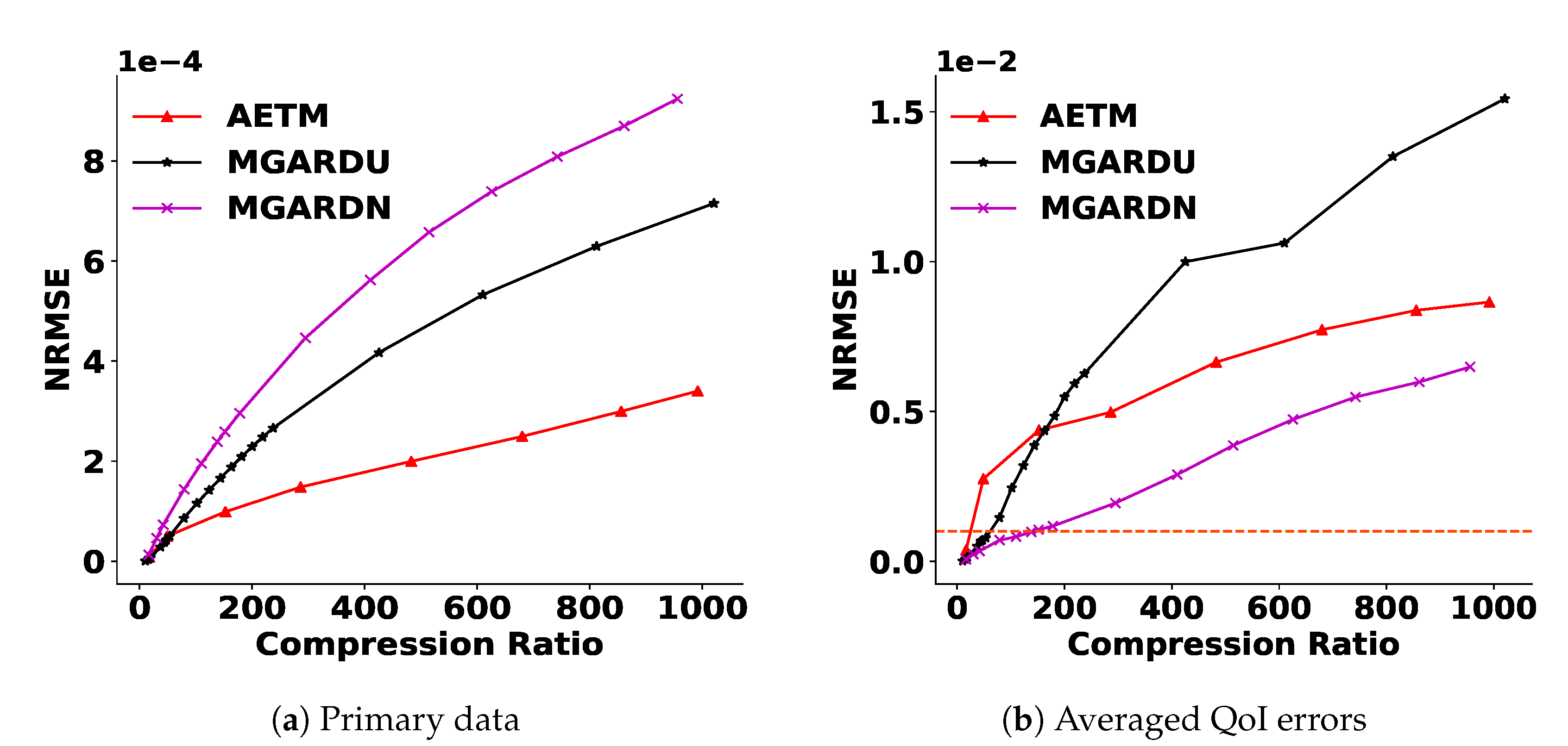
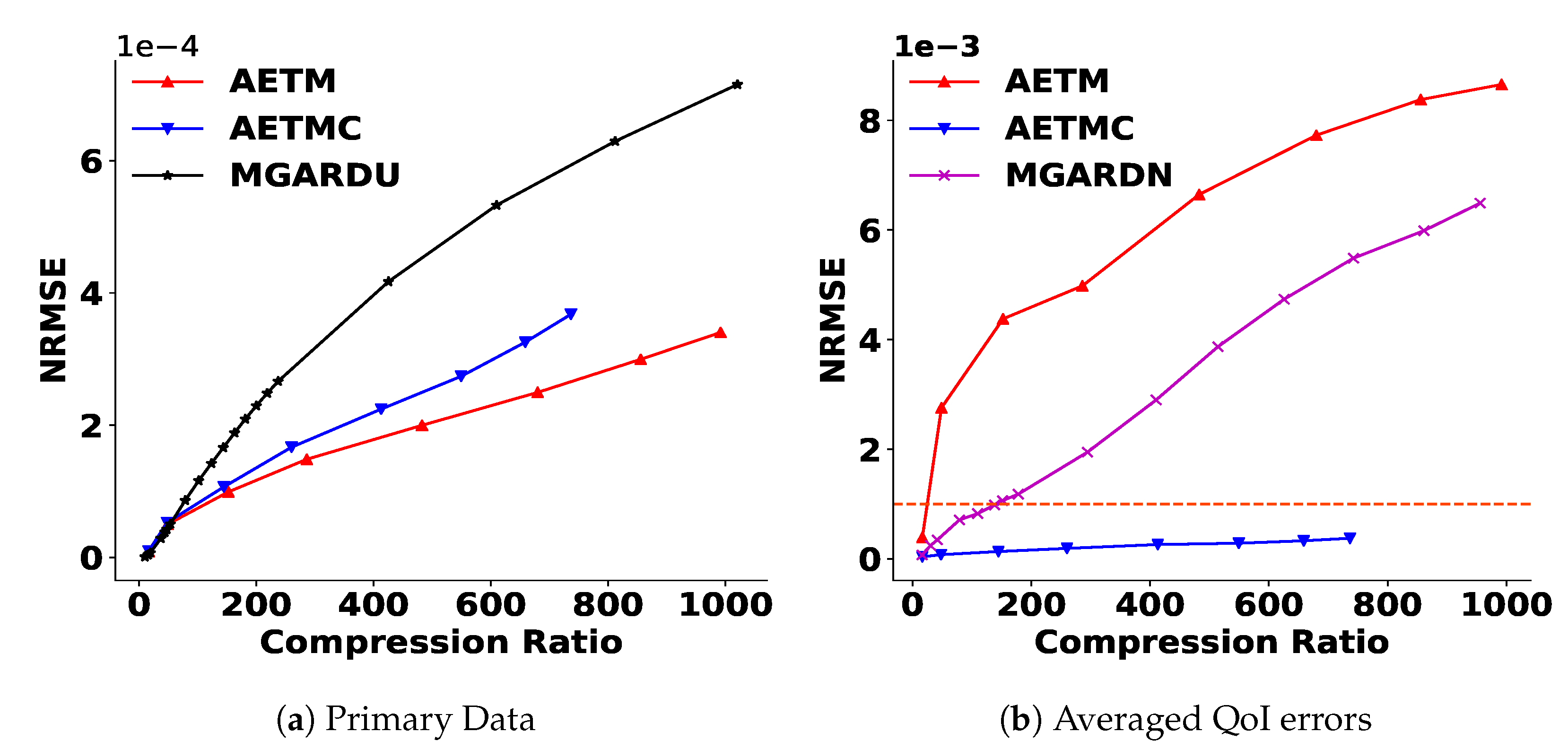
Residual post-processing enables us to guarantee the PD error in our framework. We compress residuals with MGARD to bound the reconstruction error of residuals, and thus the overall PD error is bounded. In this step, any error-bounded lossy compressors can be used. We call the reduction of PD part in our framework AETM (AET followed by MGARD). To optimize the amount of compression achieved, we limit this step to only nodes where the errors are high, and therefore it is conditional post-processing. As discussed in Section 3.1.4, the residual of a node is processed if the NRMSE of the node is larger than a user-defined PD threshold. Therefore, we can achieve different compression amounts by changing the PD threshold and MGARD error bound parameters. Figure 3a shows that the AETM outperforms the two versions of MGARD in PD NRMSE. This is due to the efficient compression in AET followed by selective residual post-processing on a subset of the output.
4.4.2. Satisfaction of Derived Quantities
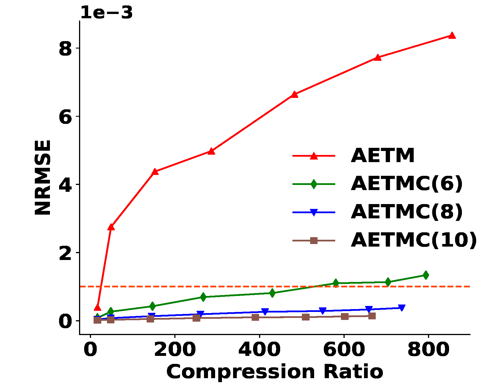
Figure 3 shows that AETM works better than MGARD uniform, but worse than MGARD non-uniform in QoI preservation. After we obtain the reconstructed output via AETM, we perform the reduction of QoI errors. We call our entire framework, including QoI satisfaction, AETMC (AETM followed by constraint satisfaction). To analyze particle simulation properties, it is crucial for XGC scientists to maintain low errors of QoI (less than 0.001 NRMSE) after decompression. As we discussed in Section 3.2.1, the QoI satisfaction process produces four Lagrange multipliers per node, and therefore we need to store four additional floating-point numbers per node. To improve storage efficiency, we use PQ to quantize the Lagrange multipliers. Hence, there is a trade-off between the amount of the reduction of the QoI errors and compression ratios as shown in Figure 4. Additionally, we need to consider the increase in PD errors after the constraint satisfaction step, as discussed in Section 3.2.1. Table 3 and Figure 5a show that the increase in PD errors is tolerable and the AETMC outperforms MGARD in PD NRMSE. Figure 5 and Figure 6 show the overall results and the performance on each QoI.
4.4.3. Framework with Test Data
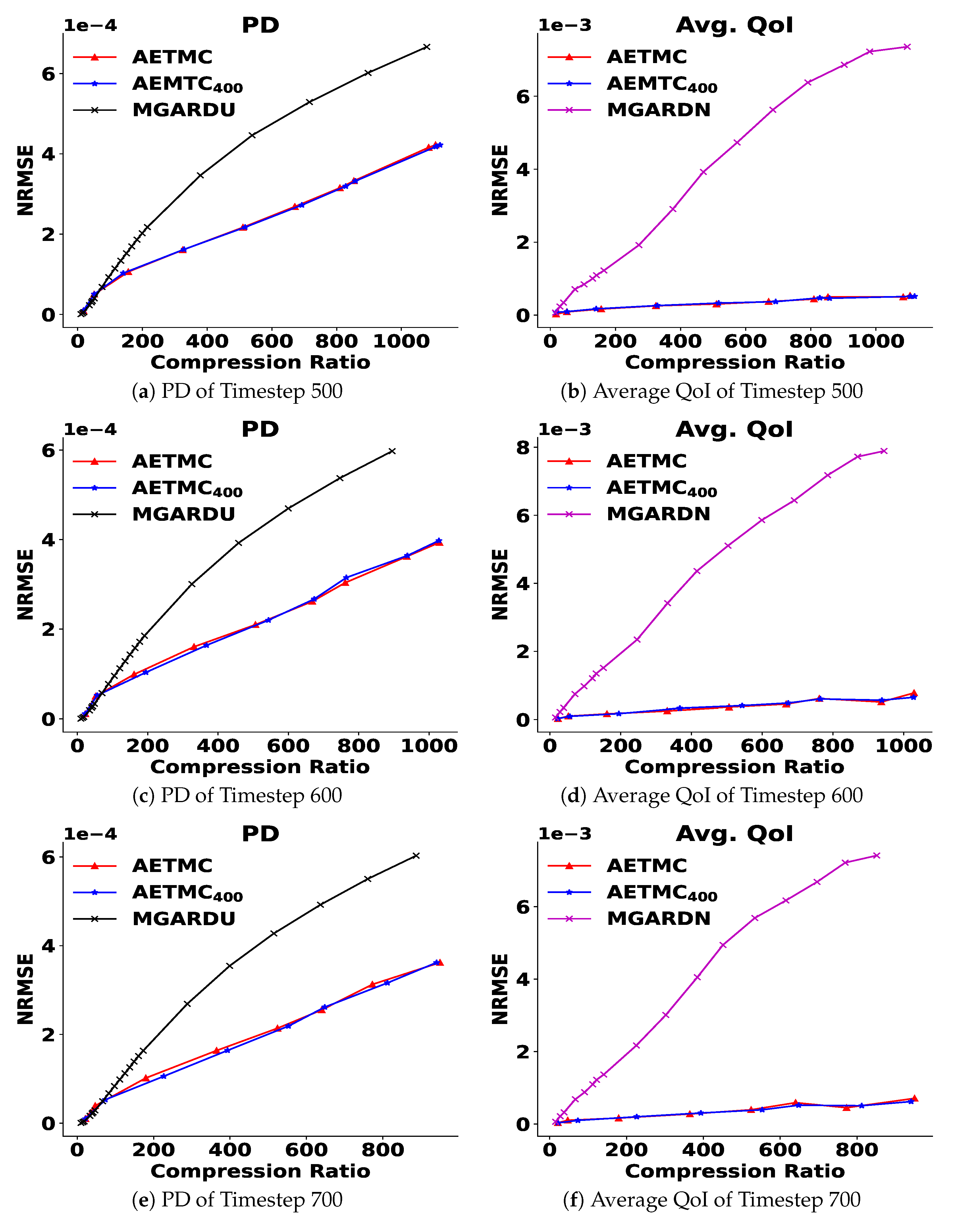
In the previous experiment, we did not split training and test data, as the case considered was static in time. However, since XGC is a spatio-temporal simulation, we now consider one set of timestep data as a training set and other set of timestep data as the test set. We first train an AE model at timestep 400 and then use the pretrained AE model to test timesteps 500, 600, and 700. Here, only the AE aspect of our framework is related to training and testing with other parts of our framework such as residual processing and constraint satisfaction, as before. Figure 7 shows the comparison between the pretrained AE model and AE models separately trained at each timestep. The results show that the performance of the pretrained model is very close to the models trained at each timestep. Consequently, this indicates that it is possible to improve machine efficiency, since the cost can be amortized across time. We plan to explore this in the future.
5. Conclusions
We have presented a comprehensive framework and a set of algorithms for error-bounded scientific data compression, which are broadly applicable to tensor datasets with moment constraints. Tucker decompositions, product quantization, and error-bounded compression are combined with an autoencoder (AE) in the framework. An AE with the Tucker decomposition can learn efficient global representations, and the reconstruction errors are bounded by selective residual post-processing with an error-bounded compressor. This leads to high levels of compression with bounded errors. Furthermore, the constraint satisfaction step enables us to reduce the errors of the QoI, and therefore the QoI are preserved during compression. The application to XGC and comparison with MGARD has shown that we can achieve compression ratios in excess of 500 while satisfying QoI error bounds. We also show that a pretrained AE model shows good performance across nearby timestep data points in the XGC simulation. Therefore, the framework can compress multiple timestep data efficiently by omitting retraining the AE model for each timestep. Immediate future work will focus on improving machine efficiency with amortization across time, and end-to-end learning machines which integrate latent space entropy estimation and constraint satisfaction. Non-linear QoI that cannot be simplified need further investigation as well. Finally, we plan to develop methods for other scientific applications (such as climate) which require error-bounded compression.
Author Contributions
Conceptualization, S.R. and S.K.; methodology, J.L. and A.R.; software, J.L., Q.G. and J.C.; validation, J.L., T.B. and Q.G.; formal analysis, J.L.; investigation, J.L.; resources, S.K.; data curation, J.C. and J.L.; writing—original draft preparation, J.L., A.R. and S.R.; writing—review and editing, J.L. and A.R.; visualization, J.L.; supervision, A.R.; project administration, S.R. and S.K.; funding acquisition, S.R. and S.K. All authors have read and agreed to the published version of the manuscript.
Funding
This research was partially supported by DOE DE-SC0022265 and DOE DE-SC0021320 RAPIDS2.
Institutional Review Board Statement
Not applicable.
Informed Consent Statement
Not applicable.
Data Availability Statement
Not applicable.
Acknowledgments
The authors acknowledge the DOE (Grant No. DE-SC0022265) and DOE RAPIDS2 (Grant No. DE-SC0021320) for funding this project.
Conflicts of Interest
The authors declare no conflict of interest.
Appendix A. Implementation Details
We implemented an autoencoder (AE) using PyTorch [43]. The network architecture and parameters we use are shown in Table A1 and Table A2. We utilize the Adam optimizer [44] with a learning rate of and set the batch size to 128. The encoder has just one fully connected layer and the weights of the decoder are the transpose of the weights of the encoder, which improves the stability of the AE and reduces the model size. There is no test set, since we need to compress all the data. Overfitting is automatically taken into consideration, since this leads to very large-size machines and lowers the compression ratio (since the size of the machine is included in the compression cost computation).

Table A1.
Autoencoder implementation. Network architecture. FC denotes a fully connected layer.
| Encoder | Decoder | |
|---|---|---|
| Layer | 1 FC | 1FC |
| Weight | ||
| Activation | Linear | Linear |
Table A2.
Network parameters.
| Parameter | Setting |
|---|---|
| Epochs | 300 |
| Learning rate | 0.001 |
| Optimizer | Adam |
Appendix B. Algorithms
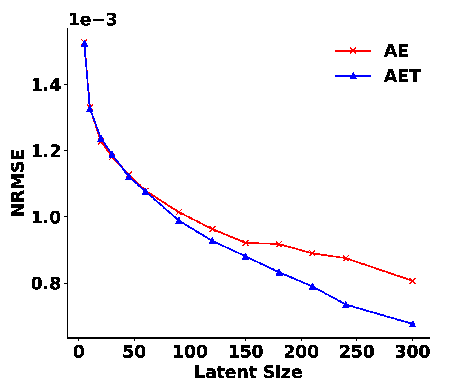
The algorithms used in the AETMC framework are described in Algorithm A1. We utilize the implementations of a product quantizer (PQ) [36] and MGARD uniform [11] in the framework. We use the Tucker decomposition as a data preprocessing step, as it can discover global correlations and provide a basis for the data. After the data are projected into the Tucker space, the AE goes to work on the core tensor coefficients with many correlations removed. Figure A1 shows that using the Tucker decomposition as a data preprocessing step improves the AE reconstruction.
Figure A1.
Improvement of PD errors with the Tucker decomposition. The x-axis is the bottleneck layer size of the AEs.
Figure A1.
Improvement of PD errors with the Tucker decomposition. The x-axis is the bottleneck layer size of the AEs.

Appendix C. Computation Time
The computation time of each component in the AETMC framework and MGARD is described in Table A3. Since we perform residual post-processing selectively, the computation time of residual post-processing is less than the running time of MGARD for the entire dataset.
Table A3.
Computation time of the AETMC framework. One set of parameters (one residual threshold and error bound) is used. For comparison, the computation time of MGARD is presented.
Table A3.
Computation time of the AETMC framework. One set of parameters (one residual threshold and error bound) is used. For comparison, the computation time of MGARD is presented.
| AETMC | MGARD | ||
|---|---|---|---|
| AE Compression | Residual Post-Processing | Constraint Satisfaction | |
| 3 min | 3 min | 30 s | 5 min |
| Algorithm A1 AETMC. | |
Input:, , and : a 16,395 × 39 × 39 tensor per each cross-section. Each represents a 2D velocity histogram. There are eight cross-sections per each timestep and each cross-section has 16,395 nodes. : a 16,395 × 4 tensor representing four true QoI values of histograms computed using per each cross-section. : geometry metadata where in Equation (21). | |
|
|
References
- Foster, I. Computing Just What You Need: Online Data Analysis and Reduction at Extreme Scales. In Proceedings of the 2017 IEEE 24th International Conference on High Performance Computing (HiPC), Jaipur, India, 18–21 December 2017; p. 306. [Google Scholar] [CrossRef] [Green Version]
- Grois, D.; Marpe, D.; Mulayoff, A.; Itzhaky, B.; Hadar, O. Performance comparison of H.265/MPEG-HEVC, VP9 and H.264/MPEG-AVC encoders. In Proceedings of the 2013 Picture Coding Symposium (PCS), San Jose, CA, USA, 8–11 December 2013; pp. 394–397. [Google Scholar] [CrossRef]
- Lindstrom, P.; Isenburg, M. Fast and Efficient Compression of Floating-Point Data. IEEE Trans. Vis. Comput. Graph. 2006, 12, 1245–1250. [Google Scholar] [CrossRef] [PubMed]
- Collet, Y.; Kucherawy, M.S. Zstandard Compression and the ‘application/zstd’ Media Type. RFC 2021, 8878, 1–45. [Google Scholar] [CrossRef]
- Lindstrom, P. Error Distributions of Lossy Floating-Point Compressors; Lawrence Livermore National Laboratory (LLNL): Livermore, CA, USA, 2017. Technical Report LLNL-CONF-740547. Available online: https://www.osti.gov/servlets/purl/1526183 (accessed on 6 June 2022).
- Di, S.; Cappello, F. Fast Error-Bounded Lossy HPC Data Compression with SZ. In Proceedings of the 2016 IEEE International Parallel and Distributed Processing Symposium (IPDPS), Chicago, IL, USA, 23–27 May 2016; pp. 730–739. [Google Scholar] [CrossRef]
- Tao, D.; Di, S.; Chen, Z.; Cappello, F. Significantly Improving Lossy Compression for Scientific Data Sets Based on Multidimensional Prediction and Error-Controlled Quantization. In Proceedings of the 2017 IEEE International Parallel and Distributed Processing Symposium (IPDPS), Orlando, FL, USA, 29 May–2 June 2017; pp. 1129–1139. [Google Scholar] [CrossRef] [Green Version]
- Liang, X.; Di, S.; Tao, D.; Li, S.; Li, S.; Guo, H.; Chen, Z.; Cappello, F. Error-Controlled Lossy Compression Optimized for High Compression Ratios of Scientific Datasets. In Proceedings of the 2018 IEEE International Conference on Big Data (Big Data), Seattle, WA, USA, 10–13 December 2018; pp. 438–447. [Google Scholar] [CrossRef]
- Lindstrom, P. Fixed-Rate Compressed Floating-Point Arrays. IEEE Trans. Vis. Comput. Graph. 2014, 20, 2674–2683. [Google Scholar] [CrossRef] [PubMed]
- Ainsworth, M.; Tugluk, O.; Whitney, B.; Klasky, S. Multilevel techniques for compression and reduction of scientific data—The univariate case. Comput. Vis. Sci. 2018, 19, 65–76. [Google Scholar] [CrossRef]
- Ainsworth, M.; Tugluk, O.; Whitney, B.; Klasky, S. Multilevel techniques for compression and reduction of scientific data—The multivariate case. SIAM J. Sci. Comput. 2019, 41, A1278–A1303. [Google Scholar] [CrossRef]
- Ainsworth, M.; Tugluk, O.; Whitney, B.; Klasky, S. Multilevel techniques for compression and reduction of scientific data-quantitative control of accuracy in derived quantities. SIAM J. Sci. Comput. 2019, 41, A2146–A2171. [Google Scholar] [CrossRef]
- Ibarria, L.; Lindstrom, P.; Rossignac, J.; Szymczak, A. Out-of-core compression and decompression of large n-dimensional scalar fields. Comput. Graph. Forum 2003, 22, 343–348. [Google Scholar] [CrossRef] [Green Version]
- Li, M.; Zuo, W.; Gu, S.; Zhao, D.; Zhang, D. Learning convolutional networks for content-weighted image compression. In Proceedings of the IEEE Conference on Computer Vision and Pattern Recognition, Salt Lake City, UT, USA, 18–22 June 2018; pp. 3214–3223. [Google Scholar] [CrossRef] [Green Version]
- Cheng, Z.; Sun, H.; Takeuchi, M.; Katto, J. Deep convolutional autoencoder-based lossy image compression. In Proceedings of the 2018 Picture Coding Symposium (PCS), San Francisco, CA, USA, 24–27 June 2018; pp. 253–257. [Google Scholar] [CrossRef] [Green Version]
- Zhou, L.; Cai, C.; Gao, Y.; Su, S.; Wu, J. Variational autoencoder for low bit-rate image compression. In Proceedings of the IEEE Conference on Computer Vision and Pattern Recognition Workshops, Salt Lake City, UT, USA, 18–22 June 2018; pp. 2617–2620. Available online: https://openaccess.thecvf.com/content_cvpr_2018_workshops/papers/w50/Zhou_Variational_Autoencoder_for_CVPR_2018_paper.pdf (accessed on 6 June 2022).
- Liu, T.; Wang, J.; Liu, Q.; Alibhai, S.; Lu, T.; He, X. High-Ratio Lossy Compression: Exploring the Autoencoder to Compress Scientific Data. IEEE Trans. Big Data 2021. [Google Scholar] [CrossRef]
- Glaws, A.; King, R.; Sprague, M. Deep learning for in situ data compression of large turbulent flow simulations. Phys. Rev. Fluids 2020, 5, 114602. [Google Scholar] [CrossRef]
- He, K.; Zhang, X.; Ren, S.; Sun, J. Deep Residual Learning for Image Recognition. In Proceedings of the 2016 IEEE Conference on Computer Vision and Pattern Recognition (CVPR), Las Vegas, NV, USA, 27–30 June 2016; pp. 770–778. [Google Scholar] [CrossRef] [Green Version]
- Karniadakis, G.E.; Kevrekidis, I.G.; Lu, L.; Perdikaris, P.; Wang, S.; Yang, L. Physics-informed machine learning. Nat. Rev. Phys. 2021, 3, 422–440. [Google Scholar] [CrossRef]
- Ling, J.; Kurzawski, A.; Templeton, J. Reynolds averaged turbulence modelling using deep neural networks with embedded invariance. J. Fluid Mech. 2016, 807, 155–166. [Google Scholar] [CrossRef]
- Wu, J.L.; Xiao, H.; Paterson, E. Physics-informed machine learning approach for augmenting turbulence models: A comprehensive framework. Phys. Rev. Fluids 2018, 3, 074602. [Google Scholar] [CrossRef] [Green Version]
- Bar-Sinai, Y.; Hoyer, S.; Hickey, J.; Brenner, M.P. Learning data-driven discretizations for partial differential equations. Proc. Natl. Acad. Sci. USA 2019, 116, 15344–15349. [Google Scholar] [CrossRef] [PubMed] [Green Version]
- De Bézenac, E.; Pajot, A.; Gallinari, P. Deep learning for physical processes: Incorporating prior scientific knowledge. J. Stat. Mech. Theory Exp. 2019, 2019, 124009. [Google Scholar] [CrossRef] [Green Version]
- Bertsekas, D. Nonlinear Programming; Athena Scientific: Chestnut, NH, USA, 1999. [Google Scholar] [CrossRef]
- Bertsekas, D.P. Constrained Optimization and Lagrange Multiplier Methods; Academic Press: Cambridge, MA, USA, 2014. [Google Scholar] [CrossRef]
- Dener, A.; Miller, M.A.; Churchill, R.M.; Munson, T.; Chang, C.S. Training neural networks under physical constraints using a stochastic augmented Lagrangian approach. arXiv 2020, arXiv:2009.07330. [Google Scholar] [CrossRef]
- Miller, M.A.; Churchill, R.M.; Dener, A.; Chang, C.S.; Munson, T.; Hager, R. Encoder–decoder neural network for solving the nonlinear Fokker–Planck–Landau collision operator in XGC. J. Plasma Phys. 2021, 87, 905870211. [Google Scholar] [CrossRef]
- Beucler, T.; Pritchard, M.; Rasp, S.; Ott, J.; Baldi, P.; Gentine, P. Enforcing analytic constraints in neural networks emulating physical systems. Phys. Rev. Lett. 2021, 126, 098302. [Google Scholar] [CrossRef]
- Wang, S.; Teng, Y.; Perdikaris, P. Understanding and mitigating gradient flow pathologies in physics-informed neural networks. SIAM J. Sci. Comput. 2021, 43, A3055–A3081. [Google Scholar] [CrossRef]
- Ku, S.; Chang, C.; Diamond, P. Full-f gyrokinetic particle simulation of centrally heated global ITG turbulence from magnetic axis to edge pedestal top in a realistic tokamak geometry. Nucl. Fusion 2009, 49, 115021. [Google Scholar] [CrossRef]
- Chang, C.; Ku, S. Spontaneous rotation sources in a quiescent tokamak edge plasma. Phys. Plasmas 2008, 15, 062510. [Google Scholar] [CrossRef]
- Hager, R.; Chang, C.S.; Ferraro, N.M.; Nazikian, R. Gyrokinetic study of collisional resonant magnetic perturbation (RMP)-driven plasma density and heat transport in tokamak edge plasma using a magnetohydrodynamic screened RMP field. Nucl. Fusion 2019, 59. [Google Scholar] [CrossRef]
- Tucker, L. Some mathematical notes on three-mode factor analysis. Psychometrika 1966, 31, 279–311. [Google Scholar] [CrossRef] [PubMed]
- Sheehan, B.N.; Saad, Y. Higher Order Orthogonal Iteration of Tensors (HOOI) and its Relation to PCA and GLRAM. In Proceedings of the 2007 SIAM International Conference on Data Mining (SDM), Minneapolis, MN, USA, 26–28 April 2007. [Google Scholar] [CrossRef] [Green Version]
- Jégou, H.; Douze, M.; Schmid, C. Product Quantization for Nearest Neighbor Search. IEEE Trans. Pattern Anal. Mach. Intell. 2011, 33, 117–128. [Google Scholar] [CrossRef] [PubMed] [Green Version]
- Gray, R. Vector quantization. IEEE ASSP Mag. 1984, 1, 4–29. [Google Scholar] [CrossRef]
- Bregman, L.M. The relaxation method of finding the common point of convex sets and its application to the solution of problems in convex programming. USSR Comput. Math. Math. Phys. 1967, 7, 200–217. [Google Scholar] [CrossRef]
- Censor, Y.; Lent, A. An iterative row-action method for interval convex programming. J. Optim. Theory Appl. 1981, 34, 321–353. [Google Scholar] [CrossRef]
- Agarap, A.F. Deep Learning using Rectified Linear Units (ReLU). arXiv 2018, arXiv:1803.08375. [Google Scholar]
- Dennis, J.; Moré, J. Quasi-Newton Methods, Motivation and Theory. SIAM Rev. 1977, 19, 46–89. [Google Scholar] [CrossRef] [Green Version]
- Rebut, P.H. ITER: The first experimental fusion reactor. Fusion Eng. Des. 1995, 30, 85–118. [Google Scholar] [CrossRef]
- Paszke, A.; Gross, S.; Massa, F.; Lerer, A.; Bradbury, J.; Chanan, G.; Killeen, T.; Lin, Z.; Gimelshein, N.; Antiga, L.; et al. PyTorch: An Imperative Style, High-Performance Deep Learning Library. In Proceedings of the Advances in Neural Information Processing Systems, Vancouver, BC, Canada, 8–14 December 2019; pp. 8026–8037. [Google Scholar] [CrossRef]
- Kingma, D.P.; Ba, J. Adam: A Method for Stochastic Optimization. arXiv 2015, arXiv:1412.6980. [Google Scholar] [CrossRef]
Figure 1.
Coordinates of the XGC dataset (left) and an example particle distribution histogram (right). The XGC simulates a massively large number of particles in a 5D physics space and regularly calculates particles distributions at each discretized node. This is one of the large datasets in XGC.
Figure 1.
Coordinates of the XGC dataset (left) and an example particle distribution histogram (right). The XGC simulates a massively large number of particles in a 5D physics space and regularly calculates particles distributions at each discretized node. This is one of the large datasets in XGC.

Figure 2.
A high-level description of the overall framework. The framework mainly consists of two parts—Primary Data (PD) reduction and Quantities of Interest (QoI) satisfaction. In the PD reduction part, we use Tucker decomposition as a preprocessing step. Then, an autoencoder (AE) compresses the Tucker basis coefficients. After training, a product quantizer (PQ) encodes the AE latent space. AET denotes the combination of Tucker decomposition, an AE, and PQ. MGARD is used for residual post-processing and it provides the guaranteed error bound on PD. AETM is AET followed by MGARD. In the QoI satisfaction step, we run constrained optimization on the reconstructed data via AETM. The purpose of this step is to directly control QoI preservation and obtain the new output, while keeping the change of the PD errors as small as possible. Another product quantizer is used to encode Lagrange multipliers obtained in this step. The overall framework is called AETMC, denoting a combination of AETM and constraint satisfaction.

Figure 3.
Reconstruction error comparison of PD (a) and the average of six QoI (b) between AETM, MGARDU, and MGARDN. The abbreviations here and in all other figures are expanded in Table 1. The horizontal line here and in Figure 4, Figure 5b and Figure 6 indicate the acceptable QoI error threshold. The graphs show that AETM outperforms the two versions of MGARD in terms of PD NRMSE, but QoI errors of AETM need to be improved.

Figure 4.
Average of six QoI errors after constraint satisfaction.

Figure 5.
Comparison of PD (a) and the average of six QoI errors (b) in AETM, AETMC, and MGARD. The graphs show that AETM with constraint satisfaction (AETMC) outperforms two versions of MGARD in both PD and QoI errors. The number of bits for Lagrange multiplier quantization in AETMC is chosen to be 8.

Figure 6.
Comparison of individual QoI between AETMC and MGARD. The graphs show that QoI errors of AETMC remain almost constant as a result of constraint satisfaction.
Figure 6.
Comparison of individual QoI between AETMC and MGARD. The graphs show that QoI errors of AETMC remain almost constant as a result of constraint satisfaction.

Figure 7.
Running the AETMC framework with test data: The AE () is trained at timestep 400 and tested at timesteps 500, 600, and 700 with comparisons against separately trained AETMC models.
Figure 7.
Running the AETMC framework with test data: The AE () is trained at timestep 400 and tested at timesteps 500, 600, and 700 with comparisons against separately trained AETMC models.

Table 1.
Table of acronyms.
| Acronyms | Meaning |
|---|---|
| PD | Primary data (original data) |
| QoI | Quantities of interest |
| AE | Autoencoder |
| PQ | Product quantizer |
| AET | Combination of Tucker decomposition, AE, and PQ |
| AETM | AET followed by MGARD for residual post-processing |
| AETMC | AETM followed by constraint satisfaction for QoI preservation |
| MGARDU | MGARD uniform |
| MGARDN | MGARD non-uniform |
Table 2.
Configuration space of our framework.
| Reduction | Components | Parameters | |||
|---|---|---|---|---|---|
| PD | AET Compression | Bottleneck layer | 5 | ⋯ | 300 |
| PQ bits | 4 | ⋯ | 12 | ||
| Residual post-processing | PD threshold | ⋯ | |||
| MGARD error bound | ⋯ | ||||
| QoI | Lagrange Multipliers | PQ bits | 6 | ⋯ | 10 |
Table 3.
Primary data error increase after constraint satisfaction. The numbers in the parentheses here and in Figure 4 are the quantization bits for Lagrange multipliers.
Table 3.
Primary data error increase after constraint satisfaction. The numbers in the parentheses here and in Figure 4 are the quantization bits for Lagrange multipliers.
| Framework | PD Error Increase |
|---|---|
| AETMC (6) | 10 |
| AETMC (8) | 9.4 |
| AETMC (10) | 9.3 |
Publisher’s Note: MDPI stays neutral with regard to jurisdictional claims in published maps and institutional affiliations. |
© 2022 by the authors. Licensee MDPI, Basel, Switzerland. This article is an open access article distributed under the terms and conditions of the Creative Commons Attribution (CC BY) license (https://creativecommons.org/licenses/by/4.0/).
Share and Cite
MDPI and ACS Style
Lee, J.; Gong, Q.; Choi, J.; Banerjee, T.; Klasky, S.; Ranka, S.; Rangarajan, A. Error-Bounded Learned Scientific Data Compression with Preservation of Derived Quantities. Appl. Sci. 2022, 12, 6718. https://doi.org/10.3390/app12136718
AMA Style
Lee J, Gong Q, Choi J, Banerjee T, Klasky S, Ranka S, Rangarajan A. Error-Bounded Learned Scientific Data Compression with Preservation of Derived Quantities. Applied Sciences. 2022; 12(13):6718. https://doi.org/10.3390/app12136718
Chicago/Turabian StyleLee, Jaemoon, Qian Gong, Jong Choi, Tania Banerjee, Scott Klasky, Sanjay Ranka, and Anand Rangarajan. 2022. "Error-Bounded Learned Scientific Data Compression with Preservation of Derived Quantities" Applied Sciences 12, no. 13: 6718. https://doi.org/10.3390/app12136718
Note that from the first issue of 2016, this journal uses article numbers instead of page numbers. See further details here.