
Estimation Method for Road Link Travel Time Considering the Heterogeneity of Driving Styles

1
School of Transportation, Southeast University, Nanjing 211189, China
2
National Demonstration Center for Experimental Road and Traffic Engineering Education, Southeast University, Nanjing 211189, China
3
Jiangsu Province Collaborative Innovation Center of Modern Urban Traffic Technologies, Southeast University, Nanjing 211189, China
*
Author to whom correspondence should be addressed.
Appl. Sci. 2022, 12(10), 5017; https://doi.org/10.3390/app12105017
Submission received: 17 March 2022
/
Revised: 2 May 2022
/
Accepted: 13 May 2022
/
Published: 16 May 2022
(This article belongs to the Topic Intelligent Transportation Systems)
Abstract
:To solve the problem of low automatic number plate recognition (ANPR) data integrity and low completion accuracy of incomplete traffic data, which affects the quality and utilization of ANPR data, this paper proposed a model for estimating the travel time of the road link that considers the heterogeneity of the driving styles. The travel time of historical road sections in the road network was extracted from ANPR data. The driving crowd was clustered through density-based spatial clustering of applications with noise (DBSCAN) based on the time slot, the number of trips, and the travel time. To avoid the excessive data difference between different classes and the distortion of the complement data, the Lagrange interpolation method was adopted to complement the missing road link travel time within each cluster. Taking Ningbo city in China as an example, the travel time completion accuracies of the proposed method and the direct interpolation method were compared. The results show that the interpolation method considering the heterogeneity of driving styles is more sufficient to increase the completion accuracy by 37.4% compared with the direct interpolation manner. The comparison result verifies the effectiveness of the proposed method and can provide more reliable data support for the construction of the transportation system.
1. Introduction
The continuous advancement of urbanization has caused many urban road transportation systems to face increasing congestion, which threatens the environment and transport efficiency [1]. To address issues such as traffic congestion, understanding the traffic state is critical at many levels of traffic management and traffic policy. With the rapid development of computer science and the progress of traffic system sensors, the collection of massive traffic data has shown its advantages in traffic decision-making [2]. ANPR is one of the decisive components of intelligent transportation systems [3]. It is often used in traffic big data analysis such as travel time estimation, OD (Origin–Destination) estimation, commuting recognition, etc. The ANPR uses image processing technology to collect vehicle information at the time of the shooting, such as shooting time, vehicle type, vehicle license plate, etc., which can obtain a large amount of traffic information [4]. There is much helpful traffic information in these data, and some characteristics related to traffic flow can be obtained through traffic data mining technology [5]. Thereby, traffic big data can be converted into readable information for traffic information prediction and management control [6]. By mining ANPR data, researchers can obtain the travel characteristics of travelers and judge the status of the transportation network, which can provide traffic managers with a reliable basis for policy design and implementation [7].
Many researchers have conducted research on ANPR data, mainly in the fields of OD estimation, travel time estimation, road traffic state estimation, etc. [8]. Jing Liu et al. proposed a dynamic OD prediction method for ANPR data and combined it with the Kalman filter framework for prediction [9]. Li Wan et al. studied the non-commuter travel demand of car commuters by using ANPR data. Suggestions were made for traffic demand and management after COVID-19 [7]. Hamid Mirzahossein et al. carried out real-time OD matrix estimation based on large-scale ANPR data and proposed an OD estimation method based on the Trip–Vehicle Matrix [10]. Mei Lam Tam et al. used real-time ANPR data to estimate the real-time traveler information system (RTIS) [11]. In the absence of real-time AVI data, the travel time of other road links can be inferred through the spatial variance–covariance between the historical travel time and the road network. Xiaoliang Ma et al. proposed an online and historical travel time prediction method based on the Extended Kalman Filter (EKF). This method uses ANPR data to quickly identify the traffic state when congestion appears or dissipates [12]. However, this method does not consider the correlation between different road links. Jie Li et al. pointed out a wavelet analysis method to identify travel time outliers extracted from Changsha ANPR data. A conclusion is drawn by comparing the two data processing methods [13]. Fangfang Zheng et al. proposed a linear relationship model between travel time and traffic characteristics such as standard deviation and skewness. Statistical analysis was performed on simulated data from a delay distribution model and real data from an ANPR camera [14].
Road link (a single segment of a road) travel time (TT) is becoming more and more essential in urban traffic travel information in nowadays society. Travel time estimation (TTE) has become a very crucial requirement. Accurate TTE is one of the core tasks of traffic modeling and is of great significance in many fields [15]. For example, providing accurate TTE can help travelers arrange travel routes reasonably, and the government and traffic management departments can perceive traffic conditions and ensure the smooth operation of traffic flow [16]. Driving styles vary widely among different drivers, so personalized TTE is meaningful for different styles of drivers. With information and personalized recommendations, individuals and fleet management companies can arrange their trips more accurately and improve the efficiency of the system [17].
In recent years, the problem of link TTE has been extensively studied [15]. According to the types of data used, existing methods can be roughly divided into two categories. The first category of methods focuses on modeling link-based data from various sources [18,19,20,21], and the other category focuses on modeling emerging trip-based data to estimate link TT [22,23,24]. Chaoyang Shi et al., proposed a TT distribution estimation method considering variance. The TT distribution is the sum of the deterministic link TT and the random turn delay at the intersection [25]. Xiaoqian Luo et al. used the data obtained by the point-to-point detector to analyze the traffic state of vehicles before the signal and estimate the arterial travel time on a more microscopic level [26]. Jinjun Tang et al. came up with an improved Markov chain method to estimate TT. This method considers the temporal and spatial correlation between road links and performed better when traffic conditions change [27]. Nonetheless, the model’s mobility is poor, and the details on the road section are not considered. Kun Tang et al. recommend a tensor-based urban TTE model based on GPS data. A third-order tensor model is established to model the TT of different road sections under other traffic conditions in a specific period [28]. The missing items in the tensor model are estimated by tensor decomposition. HongJian Wang et al. used large-scale trip data to estimate TT between origins and destinations in a very efficient manner. These adjacent trips were used to estimate TT, and experiments were performed on two large, real datasets [24]. Kunpeng Zhang et al. proposed a Trip Information Maximizing Generative Adversarial Network (T-InfoGAN) based on deep learning [29].
Through the literature review study on the estimation of the road link travel time in the past, we found that the ANPR data mainly focus on commuter vehicle recognition or trajectory recognition. Although the ANPR data contain ample information about traffic conditions, there is merely limited attention to the quality of the data [13]. Secondly, the use of ANPR data for TTE mainly focuses on mathematical methods for processing and less consideration of individual driver heterogeneity. Few studies on traffic guidance provided TTE based on user driving styles.
In this paper, we propose a road link TTE method that considers the heterogeneity of driving styles. The DBSCAN algorithm uses tensor-based urban personalized travel time modeling, and interpolation methods supplement the missing travel time items. TTE uses only limited information, i.e., urban ANPR data [30]. While performing DBSCAN on the tensor model, we estimate the travel time of road links in different periods. This method combines the spatial correlation between different road links and the heterogeneity among individual driving styles of other drivers. In addition, the variability caused by the inherent uncertainty of the urban road network is also considered.
The rest of the paper is organized as follows: Section 1 presents related work. Section 2 introduces tensor model establishment, travel time cluster analysis, and outlier supplementation. Section 3 presents a specific case study of TTE in Ningbo City, China. Finally, Section 4 summarizes the results of this work and puts forward the implication for future research.
2. Materials and Methods
2.1. Multi-Dimensional Tensor Model of Road Network Travel Time
Generally, the travel time of a vehicle passing through two adjacent detectors and can be calculated by the following formula:
where:
- is the travel time of the vehicle between road link .
- is the time when the vehicle passes detector .
- is the time when the vehicle passes detector .
However, the calculation of travel time is usually inaccurate. The ANPR equipment may record a car’s license plate repeatedly for a short time. Due to factors such as misidentification, identification failures, or driver stops, vehicle travel time is not accurately obtained. The travel time obtained after data processing and the actual value may have many errors. These data need to be revised scientifically.
The tensor model is one of the most commonly used methods to describe the multimodal correlation of data, which has been successfully applied to signal processing, pattern recognition, and personalized recommendation [28]. In recent years, methods based on tensor models have also been proven effective for processing traffic data, such as traffic flow and travel time. Personalized TTE refers to providing travel time information, considering the traffic conditions and driving behavior and habits, such as driving speed. Essentially, the driver’s driving characteristics are hidden in travel time data extracted from the ANPR data.
Considering that the complexity of the urban road network and the travel time of road links are affected by a variety of complex factors, the relationship between travel time and its influencing factors is modeled. According to the travel time data obtained in ANPR, a model with a fourth-order tensor is obtained. As is shown in Table 1, each dimension of the tensor represents the driver K, the time slot M, the road link N, and the number of trips L. The value of each item represents each driver and the number of trips L on the Nth road link in the Mth time slot of the Kth driver [28]. This approach is associated with the spatial correlation between different road links, the deviation between different drivers, and the correlation between traffic volume differences in time slots on travel time.
2.2. Driver Classification and Outlier Supplement
As Tillman and Hobbs described, driving behavior is influenced by many factors such as lifestyle and personality [31]. There are considerable discrepancies in different drivers’ driving styles. First, there are differences in the performance between different brands of vehicles, such as acceleration and deceleration. Second, there is a stark difference between the driving styles of autonomous vehicles and manually driven vehicles. Autonomous driving may be safer, energy-efficient, and more environmentally friendly than human driving. [32] There are also differences in driving habits between the young and the old [33].
For the outliers and missing values in the travel time, if the data are supplemented directly based on the comprehensive data of all driving people as the standard, it will lead to too many reference sources for the supplementary data, which may cause the additional data to be distorted. Hence, to achieve higher supplementation accuracy, it is necessary to classify the driving crowd and supplement the abnormal and missing data within each category to avoid mutual influence between data with lower correlation. We consider using the DBSCAN algorithm to identify driver or travel time heterogeneity from ANPR data. It is an effective density-based clustering method. Compared with other clustering methods, the DNSCAN algorithm can split the data into arbitrary-shaped clusters and does not require an a priori number of groups, which is, likewise, not sensitive to the order of points in the data [34]. For the travel time dataset , the basic definition of the DBSCAN algorithm is as follows [35]:
ε-close neighbor: For , the ε-close neighbor contains samples in the dataset whose distance from is not greater than ε, that is .
The core point is the point that contains no less than MinPts (a number) samples in the ε-close neighbor of the point.
If is located in the ε-close neighbor of , and is the core point, then it is defined that is directly density-reachable (DDR) by .
For and , if there is a sample sequence , where , and is DDR by , then the is density-reachable (DR) by .
For and , if s DR, then the is density-connected (DC) by .
The DBSCAN algorithm can cluster dense data of any shape, and it is not sensitive to abnormal points in the dataset, and the clustering results are not biased. In contrast, the k-means algorithm is generally only suitable for convex datasets.
The input parameters of the DBSCAN algorithm are MinPts and the radius of the ε-close neighbor, and the outputs are the clustering results and noise data of the sample points. The DBSCAN algorithm finds some clusters of DC objects to achieve the maximum density. The specific steps of the DBSCAN algorithm considering the heterogeneity of driving styles are as follows [36,37]:
- Aimlessly select one of the unprocessed objects for the sample set X. The object is a core point when there are more than MinPts points in the ε-close neighbor of .
- Amass all the objects in the sample set X that are DR to the object and regard them as a cluster.
- Over the process of DC, produce the final cluster.
- For the remaining objects, repeat steps 2 and 3 until all objects have been handled.
The number of clusters in the output results varies significantly with the input parameter values of the DBSCAN algorithm.
Due to equipment identification errors and long-term parking of vehicles on the road, there will be abounding missing values of travel time in the travel time dataset [13]. Therefore, outliers need to be identified and processed. The processing methods for missing values include deletion and interpolation. To ensure data integrity, we choose to impute it as a missing value. Generally, outliers need to be identified. There are many commonly used outlier identification methods, such as principles, box plot analysis, etc. [38].
A box chart is a commonly used statistical chart to describe the distribution of data, which is named after its shape of a box. Since the advantage of the box chart is that it is not affected by outliers and can accurately depict the discrete distribution of travel time data, we choose this box chart analysis method to identify outliers.
After the outliers are identified, they need to be supplemented. Common interpolation methods include Lagrange interpolation and Newton interpolation.
The basic idea of the Lagrange interpolation method is to rewrite the polynomial of the degree n interpolation function to be obtained in another representation and then use the interpolation conditions to determine the undetermined function, to find the interpolation polynomial [39].
Given n points , a polynomial of degree n−1 can be found, and the interpolation value can be obtained by substituting the unknown point through the polynomial, i.e.,
3. Case Study
3.1. Data Preprocessing
In Ningbo, Zhejiang Province, China, the ANPR system is installed at almost every intersection. The license plate recognition data contains the following information about each passing vehicle: The detector device number, license plate, time of passage, vehicle type, and the number of lanes. After checking the original data, we found that there are problems such as rapid vehicle speed, insufficient light, insufficient equipment recognition accuracy, etc. [13]. There is a considerable number of wrong recognition data or repeated recognition data.
The license plate recognition data used in this study derive from the urban road data in the central metropolitan area of Ningbo on 5 June 2018. We screened all data within the study area by detector device numbers. Duplicate, erroneous, and unchecked data were removed. To reduce the computer memory space occupied by the long detector device number and vehicle number in the original data, they are renamed. The travel time of each road section is extracted from the preprocessed data.
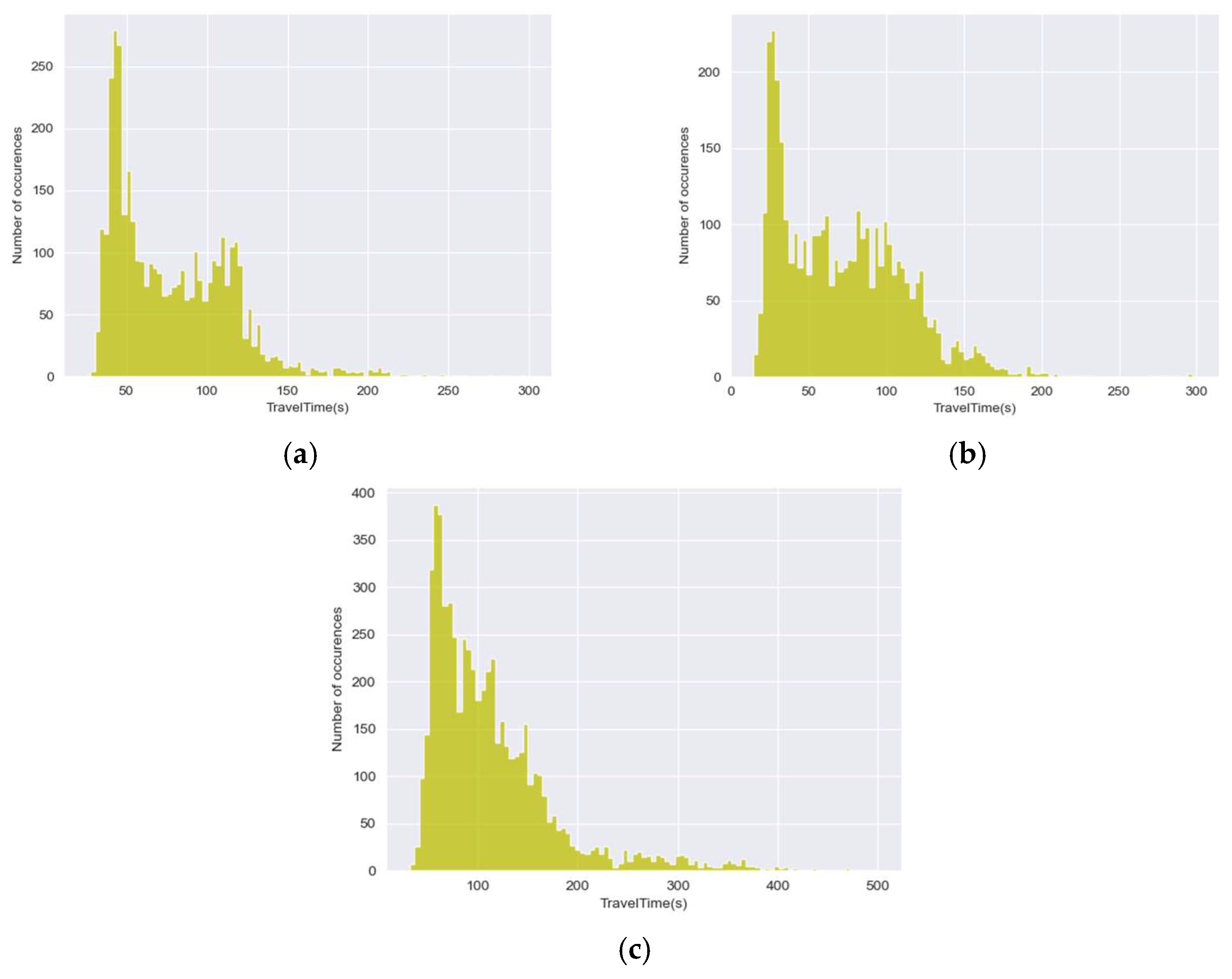
Initially, the population characteristics are analyzed based on travel time data. We selected three specific road links. The histograms of the travel time distribution frequency distribution of road links 1, 2, and 3 are shown in Figure 1. It can be seen from the figure that the travel time of most travelers is concentrated within a specific range. The peak frequency of travel time of road link 1 is concentrated at approximately 50 s, and the peak frequency of travel time of road link 2 is focused on about 40 s. The peak travel time-frequency of road link 3 is concentrated in 70–80 s. There are two frequency peaks in road links 1 and 2. The second peak of road link 1 occurred at around 115 s. The second frequency peak of road link 2 appears in about 100 s. Although the second peak in Section 3 is not apparent, it can also be observed that the second peak appears around 150 s. The travel time of most drivers on the same road link is similar. The driving time of vehicles is mainly concentrated on a particular road link, indicating that the driving time of different drivers has a certain similarity. Therefore, we consider a clustering analysis of drivers with similar travel times to study the driving characteristics of different groups of people.
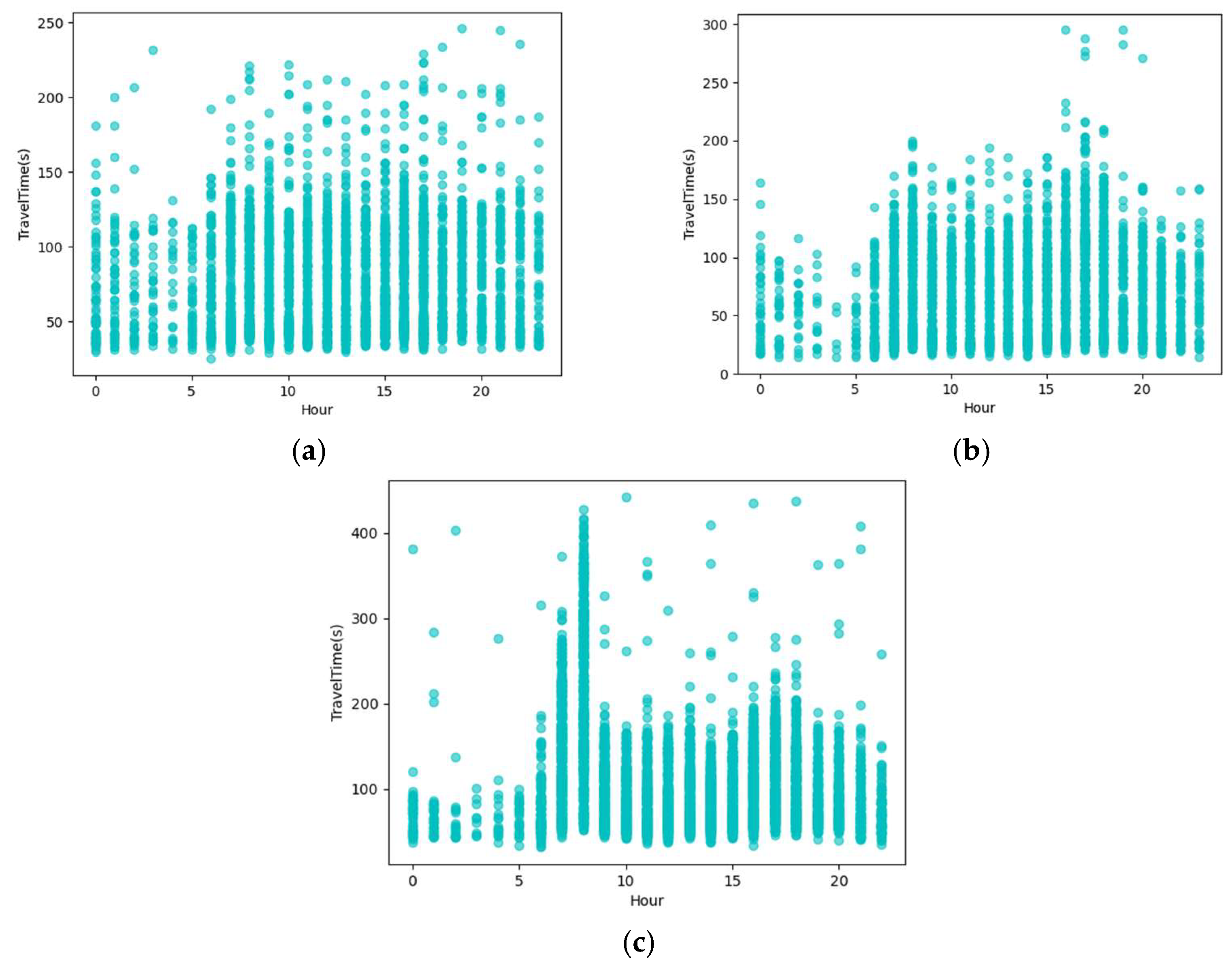
Figure 2 shows the hourly distribution of travel time for road links 1, 2, and 3. It can be seen from the figure that there is a certain similarity in the full-day travel time between three road links. The travel time of each road link is the lowest from 0 a.m. to 5 a.m. The morning peak appears from 7 a.m. to 9 p.m., and the evening peak appears from 5 p.m. to 7 p.m. It can also be seen from Figure 2c that the travel time of road link 3 at 8 a.m. is significantly longer than other periods. The sharp increase in travel time may be due to an increase in the morning rush hour, changes in signal timing, or other traffic management controls. In the meantime, there are many discrete points in the figures. These points are exceedingly different from the travel time of most vehicles, which are abnormal values of the travel time and need to be corrected.
3.2. Cluster Analysis of Drivers
The travel time of the road section is affected by various endogenous and exogenous factors. Effectively modeling the correlation between different influencing factors is a complex task. Investigation of the estimation of the travel time of the road link is conducive to improving the level of service and traffic capacity of the road link and the reasonable choice of the route by travelers.
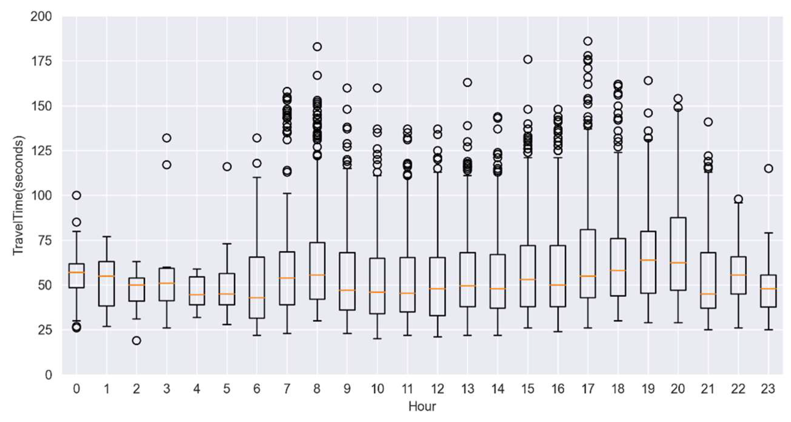
The travel time data of Road Link 1 is drawn as a box plot, as shown in Figure 3. In Figure 3, the yellow lines in the graph represent the medians. The upper and lower sides of the rectangle represent the upper quartile () and lower quartile (), respectively. The short horizontal lines at the upper and lower ends represent the upper and lower edges, respectively. The Inter Quartile Range () can be calculated by Formula (3). The points outside and are called outliers.
It can be seen from the figure that there are many discrete points in the box plot, and these points belong to abnormal values. The occurrence of these unusual points may be caused by factors such as vehicle parking, congestion, or speeding. We treat these outliers as missing values for travel time and supplement them. Some scholars have proposed an interpolation method based on accurate velocity. Although the TTE method based on accurate speed interpolation has high accuracy, it may cause severe errors on some congested road sections. The reasons may be the beginning of congestion or the evacuation of congestion [40].
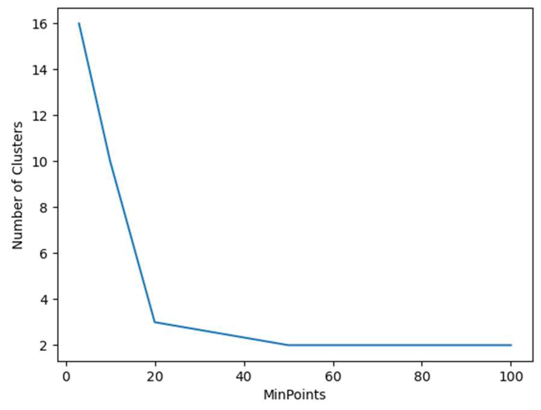
For different MinPts input values, the results of the output clusters will also be decidedly various. The input and output results of the DBSCAN algorithm are shown in Figure 4. Considering the accuracy and efficiency of the completion, 20 MinPts points and 3 types are selected as the basis for supplementing the abnormal value of the travel time.
3.3. Supplement of Travel Time Outliers
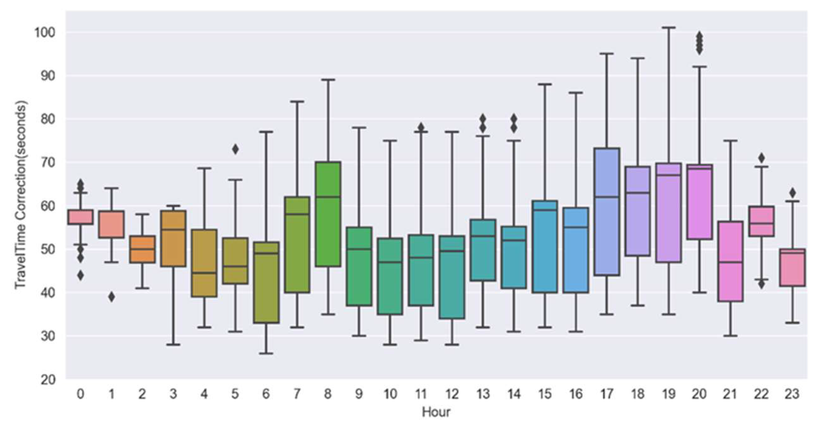
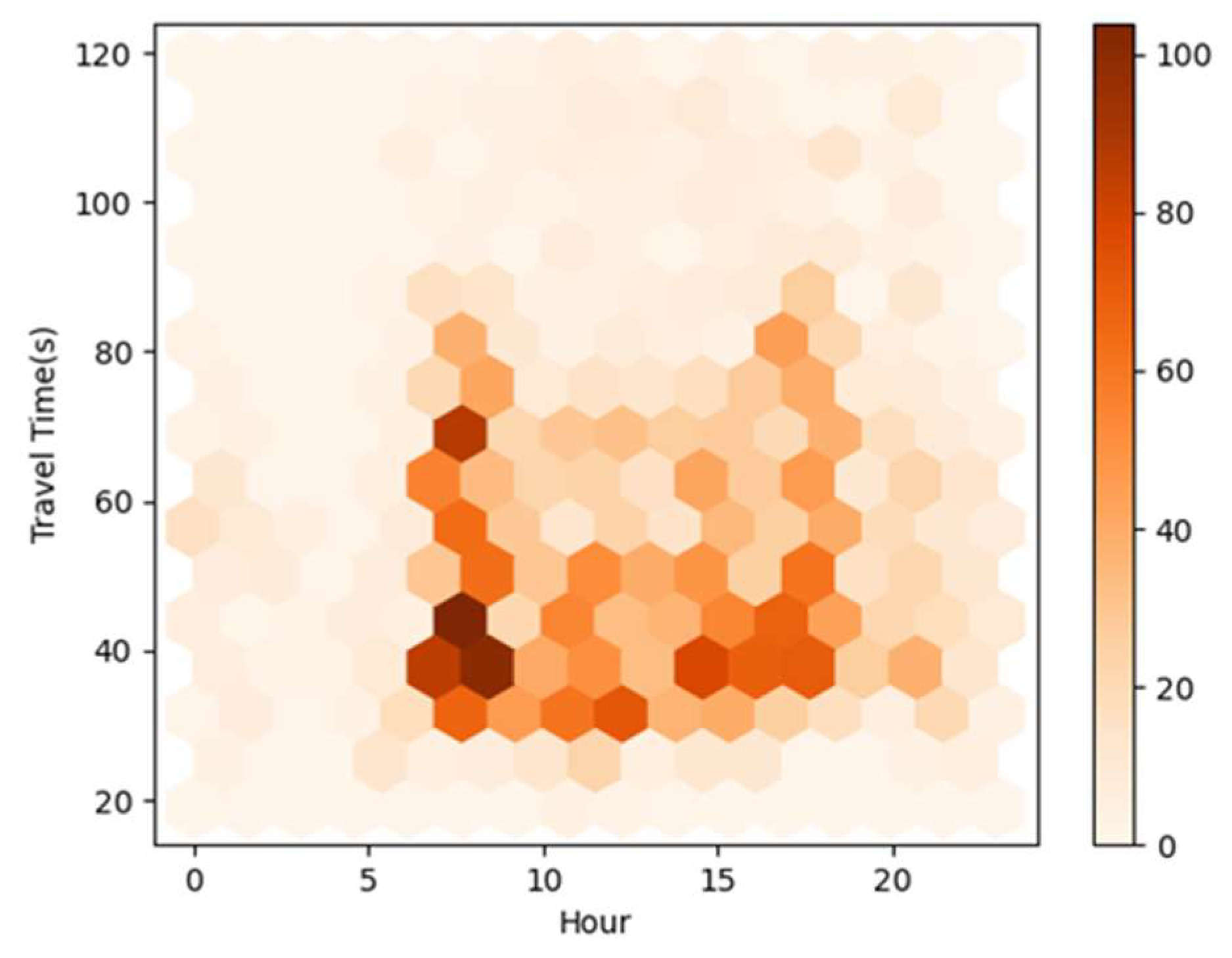
First, we use the box plot to filter out the outliers in the data, i.e., the discrete points in Figure 3. When supplementing, we determine its location beforehand. Then, we filtered out all the data with the same road link, cluster category, and time slot, and interpolated the missing travel time item based on Lagrange interpolation based on the travel time value of these data. The revised travel time results are shown in Figure 5 and Figure 6. The structure of Figure 5 is similar to that of Figure 3. Figure 6 is a Hexbin diagram of the distribution of the travel estimation results in Figure 5. The shades of color on the right represent the number of scatter points within the hexagonal area. The darker the color, the more scattered points there are in the region. Compared with Figure 3, it is not arduous to recognize that the outliers have been significantly reduced. The abnormal driving time has also been reduced to a certain extent. The missing travel time items have been better corrected.
To verify the effectiveness of the method, a method that does not consider the results of DBSCAN and directly performs interpolation is selected for comparison. Five thousand points are randomly chosen from the travel time data to estimate the travel time. The direct interpolation method and the interpolation method based on the DBSCAN results are used for comparative analysis. The results are shown in Figure 7. The abscissa is the actual value of the travel time, and the ordinate is the estimated value. The regression equations of the estimated and actual values of the two methods are, respectively:
The results show that the coefficient of the regression equation considering the difference in driving style of the crowd is closer to 1, with a larger R2 compared with the direct interpolation method. The mean value of the deviation between the estimated value and the actual value of the method proposed in this paper is 5.7 s, with a variance of 18.2 s2. In contrast, the mean value of the deviation between the estimated value of the direct interpolation method and the actual value is 9.1 s, with a variance of 44.4 s2. The accuracy of the proposed method is improved by 37.4%. It shows that the estimated travel time of the algorithm proposed in this paper is closer to the actual value, and the algorithm has a higher estimation accuracy.
4. Conclusions
ANPR data may contain relevant information such as driving habits and traffic conditions, making it possible to study the heterogeneity of traffic. This paper classifies drivers with different driving styles based on the travel time of vehicles extracted from ANPR data. According to different temporal and spatial situations, the DBSCAN algorithm is employed. The missing items of the travel time are supplemented based on the results of the clusters. The driver’s crowd heterogeneity and other factors are considered when the travel time is estimated. In this way, the TTE of the road link considering the difference in the crowd is realized. The results show that compared with the direct interpolation method, the algorithm proposed in this paper can improve the estimation accuracy by 37.4% and provide more reliable data support for subsequent transportation network research.
However, this article also has some limitations. In the tensor modeling part of this study, due to the restriction of the data format, it is not possible to obtain more attributes about the travelers themselves. Therefore, the specific attributes or characteristics of a particular driver, such as age, driving experience, etc., should be combined in follow-up research.
Author Contributions
Data curation, Y.Z. and J.Y.; funding acquisition, Y.J.; methodology, Y.Z. and J.Y.; project administration, Y.J.; resources, Y.J.; visualization, Y.Z.; writing—original draft, Y.Z.; writing—review and editing, Y.Z., Y.J. and J.Y. All authors have read and agreed to the published version of the manuscript.
Funding
This research was funded by the National Key R&D Program of China (Grant No. 2018YFE0120100 and Grant No. 2018YFB1600900), the Postgraduate Research & Practice Innovation Program of Jiangsu Province (Grant No. SJCX21_0064), and the National Demonstration Center for Experimental Road and Traffic Engineering Education (Southeast University).
Institutional Review Board Statement
Not applicable.
Informed Consent Statement
Not applicable.
Data Availability Statement
The raw automatic number plate recognition (ANPR) data used in this study are available from the corresponding author on request.
Conflicts of Interest
The authors declare no conflict of interest.
References
- Afandizadeh Zargari, S.; Memarnejad, A.; Mirzahossein, H. Hourly Origin–Destination Matrix Estimation Using Intelligent Transportation Systems Data and Deep Learning. Sensors 2021, 21, 7080. [Google Scholar] [CrossRef]
- Nejad, S.K.; Seifi, F.; Ahmadi, H.; Seifi, N. Applying Data Mining in Prediction and Classification of Urban Traffic. In Proceedings of the 2009 WRI World Congress on Computer Science and Information Engineering, Los Angeles, CA, USA, 31 March–2 April 2009; pp. 674–678. [Google Scholar]
- Mufti, N.; Shah, S.A.A. Automatic number plate Recognition: A detailed survey of relevant algorithms. Sensors 2021, 21, 3028. [Google Scholar]
- Zhang, H.; Chen, P.; Zheng, J.F.; Zhu, J.Q.; Yu, G.Z.; Wang, Y.P.; Liu, H.X. Missing data detection and imputation for urban ANPR system using an iterative tensor decomposition approach. Transp. Res. Part C Emerg. Technol. 2019, 107, 337–355. [Google Scholar] [CrossRef]
- Chen, L.; Grimstead, I.; Bell, D.; Karanka, J.; Dimond, L.; James, P.; Smith, L.; Edwardes, A. Estimating vehicle and pedestrian activity from town and city traffic cameras. Sensors 2021, 21, 4564. [Google Scholar] [CrossRef]
- He, W.; Lu, T.; Wang, E. A New Method for Traffic Forecasting Based on the Data Mining Technology with Artificial Intelligent Algorithms. Res. J. Appl. Sci. Eng. Technol. 2013, 5, 3417–3422. [Google Scholar] [CrossRef]
- Wan, L.; Tang, J.; Wang, L.; Schooling, J. Understanding non-commuting travel demand of car commuters–Insights from ANPR trip chain data in Cambridge. Transp. Policy 2021, 106, 76–87. [Google Scholar] [CrossRef]
- Ahmed, A.A.; Ahmed, S. A Real-Time Car Towing Management System Using ML-Powered Automatic Number Plate Recognition. Algorithms 2021, 14, 317. [Google Scholar] [CrossRef]
- Liu, J.; Zheng, F.; van Zuylen, H.J.; Li, J. A dynamic OD prediction approach for urban networks based on automatic number plate recognition data. Transp. Res. Procedia 2020, 47, 601–608. [Google Scholar] [CrossRef]
- Mirzahossein, H.; Gholampour, I.; Sedghi, M.; Zhu, L. How realistic is static traffic assignment? Analyzing automatic number-plate recognition data and image processing of real-time traffic maps for investigation. Transp. Res. Interdiscip. Perspect. 2021, 9, 100320. [Google Scholar] [CrossRef]
- Tam, M.L.; Lam, W.H.K. Application of automatic vehicle identification technology for real-time journey time estimation. Inf. Fusion 2011, 12, 11–19. [Google Scholar] [CrossRef]
- Ma, X.; Al Khoury, F.; Jin, J. Prediction of arterial travel time considering delay in vehicle re-identification. Transp. Res. Procedia 2017, 22, 625–634. [Google Scholar] [CrossRef]
- Li, J.; Zuylen, H.V.; Deng, Y.; Zhou, Y. Urban travel time data cleaning and analysis for Automatic Number Plate Recognition. Transp. Res. Procedia 2020, 47, 712–719. [Google Scholar] [CrossRef]
- Zheng, F.; Li, J.; Van Zuylen, H.; Liu, X.; Yang, H. Urban travel time reliability at different traffic conditions. J. Intell. Transp. Syst. 2018, 22, 106–120. [Google Scholar] [CrossRef] [Green Version]
- Sun, T.; Zhao, K.; Zhang, C.; Chen, M.; Yu, X. PR-LTTE: Link travel time estimation based on path recovery from large-scale incomplete trip data. Inf. Sci. 2022, 589, 34–45. [Google Scholar] [CrossRef]
- Jin, G.; Wang, M.; Zhang, J.; Sha, H.; Huang, J. STGNN-TTE: Travel time estimation via spatial-temporal graph neural network. Future Gener. Comput. Syst. 2021, 126, 70–81. [Google Scholar] [CrossRef]
- Jenelius, E.; Koutsopoulos, H.N. Travel time estimation for urban road networks using low frequency probe vehicle data. Transp. Res. Part B Methodol. 2013, 53, 64–81. [Google Scholar] [CrossRef] [Green Version]
- Lv, Z.; Xu, J.; Zheng, K.; Yin, H.; Zhao, P.; Zhou, X. Lc-rnn: A deep learning model for traffic speed prediction. In Proceedings of the Twenty-Seventh International Joint Conference on Artificial Intelligence, Stockholm, Sweden, 13–19 July 2018; p. 27. [Google Scholar]
- Chen, M.; Liu, Y.; Yu, X. Nlpmm: A next location predictor with markov modeling. In Pacific-Asia Conference on Knowledge Discovery and Data Mining; Springer: Cham, Germany, 2014; pp. 186–197. [Google Scholar]
- Yuan, H.; Li, G.; Bao, Z.; Feng, L. Effective travel time estimation: When historical trajectories over road networks matter. In Proceedings of the 2020 ACM Sigmod International Conference on Management of Data, Portland, OR, USA, 14–19 June 2020; pp. 2135–2149. [Google Scholar]
- Chen, M.; Zuo, Y.; Jia, X.; Liu, Y.; Yu, X.; Zheng, K. CEM: A convolutional embedding model for predicting next locations. IEEE Trans. Intell. Transp. Syst. 2020, 22, 3349–3358. [Google Scholar] [CrossRef]
- Zhan, X.; Hasan, S.; Ukkusuri, S.V.; Kamga, C. Urban link travel time estimation using large-scale taxi data with partial information. Transp. Res. Part C Emerg. Technol. 2013, 33, 37–49. [Google Scholar] [CrossRef]
- Zhan, X.; Ukkusuri, S.V.; Yang, C. A Bayesian mixture model for short-term average link travel time estimation using large-scale limited information trip-based data. Autom. Constr. 2016, 72, 237–246. [Google Scholar] [CrossRef] [Green Version]
- Wang, H.; Tang, X.; Kuo, Y.-H.; Kifer, D.; Li, Z. A simple baseline for travel time estimation using large-scale trip data. ACM Trans. Intell. Syst. Technol. (TIST) 2019, 10, 1–22. [Google Scholar] [CrossRef] [Green Version]
- Shi, C.; Chen, B.Y.; Li, Q. Estimation of travel time distributions in urban road networks using low-frequency floating car data. ISPRS Int. J. Geo-Inf. 2017, 6, 253. [Google Scholar] [CrossRef]
- Luo, X.; Wang, D.; Ma, D.; Jin, S. Grouped travel time estimation in signalized arterials using point-to-point detectors. Transp. Res. Part B Methodol. 2019, 130, 130–151. [Google Scholar] [CrossRef]
- Tang, J.; Hu, J.; Hao, W.; Chen, X.; Qi, Y. Markov Chains based route travel time estimation considering link spatio-temporal correlation. Phys. A Stat. Mech. Appl. 2020, 545, 123759. [Google Scholar] [CrossRef]
- Tang, K.; Chen, S.Y.; Liu, Z.Y. Citywide Spatial-Temporal Travel Time Estimation Using Big and Sparse Trajectories. IEEE Trans. Intell. Transp. Syst. 2018, 19, 4023–4034. [Google Scholar] [CrossRef]
- Zhang, K.; Jia, N.; Zheng, L.; Liu, Z. A novel generative adversarial network for estimation of trip travel time distribution with trajectory data. Transp. Res. Part C Emerg. Technol. 2019, 108, 223–244. [Google Scholar] [CrossRef]
- Tang, K.; Chen, S.; Liu, Z.; Khattak, A.J. A tensor-based Bayesian probabilistic model for citywide personalized travel time estimation. Transp. Res. Part C Emerg. Technol. 2018, 90, 260–280. [Google Scholar] [CrossRef]
- Tillmann, W.A.; Hobbs, G. The accident-prone automobile driver: A study of the psychiatric and social background. Am. J. Psychiatry 1949, 106, 321–331. [Google Scholar] [CrossRef]
- Gasser, T.M.; Arzt, C.; Ayoubi, M.; Bartels, A.; Bürkle, L.; Eier, J.; Flemisch, F.; Häcker, D.; Hesse, T.; Huber, W. Legal consequences of an increase in vehicle automation. In Proceedings of the Transportation Research Board 91st Annual Meeting, Washington, DC, USA, 22–26 January 2012. [Google Scholar]
- Hartwich, F.; Beggiato, M.; Krems, J.F. Driving comfort, enjoyment and acceptance of automated driving–effects of drivers’ age and driving style familiarity. Ergonomics 2018, 61, 1017–1032. [Google Scholar] [CrossRef]
- He, Y.B.; Tan, H.Y.; Luo, W.M.; Mao, H.J.; Ma, D.; Feng, S.Z.; Fan, J. Mr-dbscan: An Efficient Parallel Density-based Clustering Algorithm using MapReduce. In Proceedings of the 2011 IEEE 17th International Conference on Parallel and Distributed Systems, Tainan, Taiwan, 7–9 December 2011; pp. 473–480. [Google Scholar]
- Wang, C.X.; Ji, M.; Wang, J.; Wen, W.; Li, T.; Sun, Y. An Improved DBSCAN Method for LiDAR Data Segmentation with Automatic Eps Estimation. Sensors 2019, 19, 172. [Google Scholar] [CrossRef] [Green Version]
- Sander, J.; Ester, M.; Kriegel, H.P.; Xu, X.W. Density-based clustering in spatial databases: The algorithm GDBSCAN and its applications. Data Min. Knowl. Discov. 1998, 2, 169–194. [Google Scholar] [CrossRef]
- Duan, L.; Xu, L.; Guo, F.; Lee, J.; Yan, B. A local-density based spatial clustering algorithm with noise. Inf. Syst. 2007, 32, 978–986. [Google Scholar] [CrossRef]
- McKinney, W. Python for Data Analysis; O’Reilly Media, Inc.: Newton, MA, USA, 2013. [Google Scholar]
- Atangana, A.; Araz, S.İ. 2-Two-steps Lagrange polynomial interpolation: Numerical scheme. In New Numerical Scheme with Newton Polynomial; Academic Press: Cambridge, MA, USA, 2021; pp. 11–112. [Google Scholar]
- Soriguera Martí, F. Accuracy of Travel Time Estimation Methods Based on Punctual Speed Interpolations. In Highway Travel Time Estimation with Data Fusion; Springer: Berlin/Heidelberg, Germany, 2016. [Google Scholar]
Figure 1.
Frequency histograms of travel time distribution. (a) Road Link 1. (b) Road Link 2. (c) Road Link 3.
Figure 1.
Frequency histograms of travel time distribution. (a) Road Link 1. (b) Road Link 2. (c) Road Link 3.

Figure 2.
Hourly distribution of travel time. (a) Road Link 1. (b) Road Link 2. (c) Road Link 3.

Figure 3.
Box plot of travel time distribution in each hour within a day (for road link 1).

Figure 4.
The output results of the number of DBSCAN algorithm clusters correspond to different input MinPts values.
Figure 4.
The output results of the number of DBSCAN algorithm clusters correspond to different input MinPts values.

Figure 5.
Hourly distribution of completed travel time.

Figure 6.
Travel time estimation results of hourly density distribution.

Figure 7.
Comparison of the actual values and estimation values of two methods. (a) The results of the direct interpolation method. (b) The results of the interpolation method based on the DBSCAN results.
Figure 7.
Comparison of the actual values and estimation values of two methods. (a) The results of the direct interpolation method. (b) The results of the interpolation method based on the DBSCAN results.


Table 1.
Examples of tensor model.
| CarID | Travel Time (Second) | Hour | Road Link | Number of Trips |
|---|---|---|---|---|
| 1 | 51 | 12 | 33-22 | 5 |
| 1 | 67 | 12 | 22-75 | 5 |
| 1 | 255 | 12 | 75-98 | 5 |
| 1 | 8558 | 12 | 98-34 | 5 |
| 1 | 32 | 15 | 34-78 | 5 |
Publisher’s Note: MDPI stays neutral with regard to jurisdictional claims in published maps and institutional affiliations. |
© 2022 by the authors. Licensee MDPI, Basel, Switzerland. This article is an open access article distributed under the terms and conditions of the Creative Commons Attribution (CC BY) license (https://creativecommons.org/licenses/by/4.0/).
Share and Cite
MDPI and ACS Style
Zhang, Y.; Ji, Y.; Yu, J. Estimation Method for Road Link Travel Time Considering the Heterogeneity of Driving Styles. Appl. Sci. 2022, 12, 5017. https://doi.org/10.3390/app12105017
AMA Style
Zhang Y, Ji Y, Yu J. Estimation Method for Road Link Travel Time Considering the Heterogeneity of Driving Styles. Applied Sciences. 2022; 12(10):5017. https://doi.org/10.3390/app12105017
Chicago/Turabian StyleZhang, Yuhui, Yanjie Ji, and Jiajie Yu. 2022. "Estimation Method for Road Link Travel Time Considering the Heterogeneity of Driving Styles" Applied Sciences 12, no. 10: 5017. https://doi.org/10.3390/app12105017
Note that from the first issue of 2016, this journal uses article numbers instead of page numbers. See further details here.