
Synthetic Data Generation for the Development of 2D Gel Electrophoresis Protein Spot Models


Department of Electronic Systems, Vilnius Gediminas Technical University (VILNIUS TECH), 03227 Vilnius, Lithuania
Appl. Sci. 2022, 12(9), 4393; https://doi.org/10.3390/app12094393
Submission received: 23 March 2022
/
Revised: 22 April 2022
/
Accepted: 26 April 2022
/
Published: 27 April 2022
(This article belongs to the Special Issue Deep Learning in Bioinformatics and Biomedicine)
Abstract
:Two-dimensional electrophoresis gels (2DE, 2DEG) are the result of the procedure of separating, based on two molecular properties, a protein mixture on gel. Separated similar proteins concentrate in groups, and these groups appear as dark spots in the captured gel image. Gel images are analyzed to detect distinct spots and determine their peak intensity, background, integrated intensity, and other attributes of interest. One of the approaches to parameterizing the protein spots is spot modeling. Spot parameters of interest are obtained after the spot is approximated by a mathematical model. The development of the modeling algorithm requires a rich, diverse, representative dataset. The primary goal of this research is to develop a method for generating a synthetic protein spot dataset that can be used to develop 2DEG image analysis algorithms. The secondary objective is to evaluate the usefulness of the created dataset by developing a neural-network-based protein spot reconstruction algorithm that provides parameterization and denoising functionalities. In this research, a spot modeling algorithm based on autoencoders is developed using only the created synthetic dataset. The algorithm is evaluated on real and synthetic data. Evaluation results show that the created synthetic dataset is effective for the development of protein spot models. The developed algorithm outperformed all baseline algorithms in all experimental cases.
1. Introduction
Two-dimensional polyacrylamide gel electrophoresis (2D PAGE, 2DGE, 2DE) is the technique used to analyze complex mixtures of proteins [1,2]. By using this technique, molecules can be separated on 2D gels according to two properties: isoelectric point and molecular mass. After staining, a protein spot pattern in the 2D gel may be observed. The integrated intensity of the spot is related to the amount of protein in the area of the spot. Comparisons of 2DGE images, i.e., comparisons of the integrated intensities of the corresponding spots, can be performed to estimate the levels of expression (and its changes) of each protein in different samples [3,4,5,6].
In recent years, the popularity of 2DGE began to decrease due to the numerous advantages of other gel-free separation techniques and the progress made in their development [7,8,9]. However, the disappearance of the technique is not expected [10,11,12]. It is said that 2DGE is suitable for the new wave of top-down functional proteomics. Gel-based and gel-free approaches complement each other [10]. In addition, researchers proposed several examples of alternative applications of 2DE [13]: serological proteome analysis (SERPA) [14], two-dimensional zymography (2DZ) [15], two-dimensional immobilized metal affinity electrophoresis (2-D IMAEP) [16], and three-dimensional blue native/IEF/SDS-PAGE (3D BN/SDS-PAGE) [17].
To extract the required information from 2DE gels, images of the gels must be analyzed to detect corresponding spots and evaluate differences in the integrated intensities of corresponding spots [18,19,20,21]. This expression information, combined with the protein from the spot identification data, provides insights into the biological processes happening in the source of the protein mixture sample. Analysis of 2DGE images consists of spot detection and image alignment (if spots are detected after 2DGE image alignment) or spot matching (if 2DGE images are aligned after spot detection and spot coordinates are used to find corresponding spots) tasks [22,23,24,25,26,27].
The importance of the task of protein spot detection in the 2DGE images is that the accuracy of the detection information (spot position, area, and integrated intensity) determines the conclusions that are drawn about the biological processes that interest the researchers [28,29,30]. In order to maximize the quality of information gathered on the biological processes, the accuracy of the protein spot detection must be maximized.
A straightforward approach to improving protein spot quantification (estimation of the spot’s integrated intensity) is to develop a better segmentation algorithm that finds the boundaries of the spot and accurately removes noise (background and other intensity distortions) [31,32,33,34,35,36,37,38,39,40,41]. Spot modeling can accomplish both of these tasks simultaneously. By fitting a mathematical model to the image patch where the spot is located, high-frequency noise can be canceled, and the resulting model can be decomposed into the spot’s intensity and background’s intensity. The integration of the spot’s intensity in the region of the spot provides an estimate of integrated spot intensity. The most common models for modeling protein spots are Gaussian [41,42,43,44] and diffusion [45]. Several other models have been proposed to better approximate spots of more complex shapes [46,47].
An algorithm for protein spot modeling or reconstruction can be based on machine learning (ML) models [48]. The development of ML model-based image analysis algorithms requires a large amount of labeled training data. The acquisition of high-quality training data has its own costs. The shortcomings of real datasets are: the time-consuming data gathering and labeling process, errors or inaccuracies in label data, a limited number of samples in the dataset, a lack of diversity, difficulties in obtaining rare but crucial corner cases, and uneven representation of the features. These shortcomings may be overcome by creating synthetic datasets [44]. Of course, the simulation of data has its own difficulties. The most important is the problem of how to generate data that reflect the essential statistical properties of the underlying real-world data. However, it is predicted that, by 2030, most of the data used in AI will be artificially generated by rules, statistical models, simulations, or other techniques [49].
This work proposes a method for creating a synthetic dataset of protein spots and uses the created dataset to develop a spot modeling algorithm.
The novelty and contributions of this work can be summarized as follows:
- Proposed a method to generate a dataset consisting of synthetic protein spot image samples of high fidelity;
- Developed a new spot modeling algorithm based on autoencoders, using purely the created synthetic dataset;
- Performed a comparative evaluation of the developed protein spot modeling algorithm and other commonly used spot models using synthetic and real data;
- Experimentally showed that the created synthetic dataset is effective and sufficient for the development of protein spot models;
- Publicly provided the synthetic spot dataset generated according to the presented method.
The problem of analyzing 2DGE images and the challenges encountered during the analysis are summarized in Figure 1.
2. Materials and Methods
In this section, the proposed method for generating synthetic protein spot image data is elaborated, including the formulated requirements for the synthetic protein spot data; the methodology for the evaluation of the synthetic dataset is presented based on trained autoencoders for spot modeling, baseline models (other common protein spot models), and synthetic and real protein spot test data; and the experimental data collection process is described.
2.1. Generation of Synthetic Protein Spot Images
2.1.1. Requirements for the Synthetic Protein Spot Data
The main, challenging goal of generating synthetic data is to create useful synthetic data that reflect the important statistical properties of the underlying real-world data so that the synthetic dataset helps train better machine learning (ML) models. There are requirements for the dataset and evaluation criteria needed to develop a suitable dataset.
The requirements for the synthetic dataset arise from the purpose for which the dataset is intended. Thus, the main requirement is that the synthetic dataset must allow the development of an ML model that is well-performing on real data. This is possible to test only once the dataset is created. To speed up the process of developing the data simulation method, additional requirements that frame the early-phase dataset are formulated. Domain knowledge helps to formulate the aforementioned requirements.
Domain knowledge helps to identify the generating factors that determine the appearance of the spot. By simulating these factors, it is possible to create a synthetic patch of a 2DGE image. Thus, the small region of the 2DGE image, containing a single protein spot, can be decomposed into a pure protein spot without background, non-uniform background (low-frequency noise), and high-frequency noise (Gaussian and impulsive noise). The pure protein spot is the signal we want to measure. Its integrated intensity is correlated with the amount of protein accumulated in the spot’s area in the 2DE gel. Background and some other types of noise appear due to the staining of non-protein substances in the gel. Other sources of noise are dust and imaging conditions. A realistic input image should be simulated, including all the factors that form a real image, but the target image should contain only the protein spot of interest (only the signal, without any noise). Another observation about the appearance of the 2DGE image is that protein spots typically appear in groups. Clearly, isolated spots are not so common. Thus, secondary spots should be treated as any other noise components.
The appearance of the protein spot is typically circularly symmetric if the spot is small. The larger spots tend to possess horizontal symmetry but less vertical symmetry and have longer tails in the upright direction. This asymmetry is caused due to movement of the larger amount of protein from the top towards the bottom in the gel. The spots with large amounts of proteins appear saturated. With these observations, we want to create spots whose horizontal (intensity) sections are smooth. Examples of unwanted artifacts of spot shape construction, as well as the preferred case, are visualized in Figure 2.
Other requirements for the image patch (technical requirements) are the size of the image and the positioning of the spots in the image. Considering that the dataset is meant to develop a spot reconstruction algorithm, the image patches are selected to be small, and the main spot is centered in the image with slight variations in position. Based on the data flow in the selected ML model (input images are downsampled three times) and the attempt to balance the complexity and capacity of the ML model (in order to represent sufficiently detailed protein spots), the image patch size was set to px.
In order to develop protein spot reconstruction algorithms that are capable of reconstructing spots either without background or with remaining background, the dataset has two types or target images: one containing only the main spot (without any noise) and one containing the spot and the constant background (noise). The developed reconstruction algorithm that outputs the main spot with the background noise is used to test it on real 2DGE images because the true background intensity in the real images is unknown, and we want to measure only the ability of the trained model to replicate the appearance of real spots.
It is very important to be able to evaluate the synthetic dataset both during its development and after it is constructed in order to tell whether the dataset fulfills the formulated requirements. During the dataset’s development, we need clues as to whether we are making the right decisions regarding the simulation of properties of real-world data so that our solutions lead to the creation of a synthetic dataset that captures the properties of real and realistic data that helps to develop more accurate ML models. After the synthetic dataset is created, we need to be sure that the dataset is either helping to train better ML models or allowing the creation of ML models with fewer resources than what is required to create datasets of real data while maintaining comparable accuracy. Two evaluation approaches may be adopted: subjective evaluation and objective evaluation.
Subjective evaluation can be performed visually (perceptually) and involves trying to tell whether the generated 2DGE image patches look realistic. This evaluation method is useful during the development of the synthetic data generation method. Objective evaluation and criteria are used to test the final version of the dataset and check how well the synthetic data allow the training of an ML model. More details about the evaluation of the dataset after its creation are provided and discussed in Section 2.2.
2.1.2. Method for Generating the Synthetic Spot Image Dataset
In this section, the proposed method for synthetic protein spot image generation is described in detail. An overview of the workflow is presented in Figure 3, with an extension in Figure 4, where the first step of the main workflow is explained in more detail.
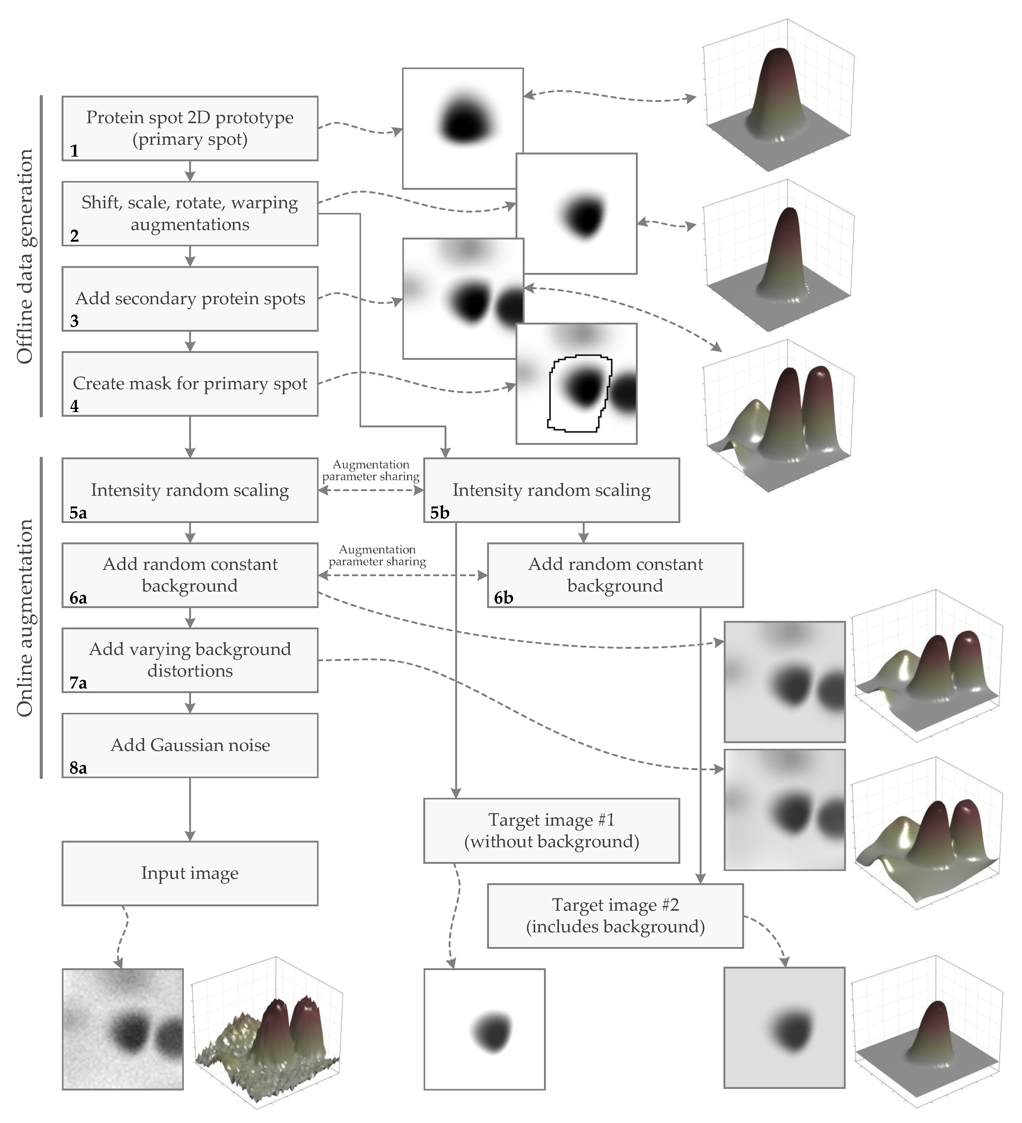
The entire image generation process may be split into two separate stages: offline data generation and online data augmentation. Offline data generation is performed before the training of the artificial neural network (ANN, NN)-based protein spot model and includes steps that are more computationally demanding. Online data augmentation is performed during the training process and includes computations that are relatively fast and are more worthwhile to perform on the fly rather than keeping precomputed. So the described stages emerge from the efforts to balance the computational load in such a way that the total computational load (or required time) to develop a neural network model for the spot reconstruction task would be minimal.
The dataset of the protein spot synthetic images comprises image pairs of an input image and a target image. The input image is a mixture of one primary spot of protein (the signal) and different numbers of secondary spots, high-frequency noise, and varying background (the noise). Input images should be as similar to real 2DE images as possible. The target image contains only the signal part of the input image. The target image is one of two types: including the constant background or without the background. These different targets are used for the development and comparison of slightly different spot reconstruction methods, where one is trained to reconstruct spots with background, and the other is trained to reconstruct spots without background (trained to remove the background).
The steps of the dataset generation workflow (Figure 3) are explained in more detail below.
1. Creation of the protein spot 2D prototype (primary spot). In this step, a primary protein spot is generated. The details of spot creation are summarized in Figure 4 and discussed in Section 2.1.3.
The prototype of the protein spot serves as a seed for generating final spots. The final appearance of the spot is determined during the next step, where geometric transformations are randomly selected and applied.
2. Implement shift, scale, rotate, and warping augmentations. This step creates the final appearance of the primary spot (or the signal), and only the maximum intensity of the spot is randomly scaled during the online augmentation. The remaining steps are used for the generation of the noise component of the 2DE image sample.
At this step, all augmentations that fall under the geometric transformations category are performed. Some of these transformations can be done during the creation of the protein spot prototype (the previous step), e.g., by randomly sampling the center position of the spot, but for the simplicity of the generation process, all the geometric transforms are performed at this step.
The transformations are created using the Albumentations library [50] (https://albumentations.ai (accessed on 1 February 2022) ). The library is designed for fast and flexible image augmentation. The augmentation includes the following geometric transforms from the Albumentations library: ShiftScaleRotate, GridDistortion, PiecewiseAffine, and OpticalDistortion.
ShiftScaleRotate randomly applies affine transforms: it translates, scales, and rotates the image. The parameters of the transformation are as follows: the shift factor range for both height and width is , the scaling factor range is , the rotation angle range in degrees is , bicubic interpolation, and image padding (border mode) is set to constant. The parameters of the GridDistortion transform are as follows: the count of grid cells on each side is 5, the distortion limit is , bicubic interpolation, and image padding (border mode) is set to constant. PiecewiseAffine applies affine transformations that differ between local neighborhoods, creating local distortions. The parameters of the transform are as follows: the scale factor range is , the number of rows (and columns) of points that the regular grid should have is 4, and bicubic interpolation. The parameters of the OpticalDistortion transform are as follows: the distortion limit is , bicubic interpolation, and image padding (border mode) is set to constant.
The probabilities of each transformation occurrence in the final augmentation pipeline are as follows: ShiftScaleRotate ; GridDistortion, PiecewiseAffine, and OpticalDistortion equally .
3. Add secondary protein spots. The existence of a lonely protein spot in the 2DE image region is a rare case. It is common that spots appear in groups with smaller or larger distances between them. If the distance is very small, spots may appear to overlap. This step of data generation simulates the real presence of protein spots in the 2DE gel. The secondary spots in the current image patch are treated as noise that should be removed during spot reconstruction.
The simulation of secondary spots is performed using the same modeling operations used for creating the primary spots. However, the spots’ centers are allowed to appear only in the 6px border area of the image patch. A maximum of 8 and minimum of 0 secondary spots may be placed in the border region. The number of secondary spots is determined randomly. The locations of the spots is also randomized but distributed on the border. The generated images with secondary spots and the main image are combined using the summation operation.
4. Create the mask for the primary spot. The mask of the primary spot defines the image region where the primary spot is located. Similar masks are created while analyzing real 2DE images. The image is decomposed into separate regions where each region contains a single spot. After that, each region is modeled in order to parameterize the spot. This created mask is used for spot modeling using common spot mathematical models.
The mask is created by segmenting the image using Watershed transform [51]. The Watershed transform splits the image so that each region contains a single local minimum. The 2DE image must be in the form of dark spots with a light background in order for the segments to be generated properly. After the Watershed transformation, only the center-most region is selected as the spot mask.
5. Perform intensity random scaling. The spots may appear to be of various intensities, from very weak to spanning the full intensity range. The intensities of the image samples containing the generated spots are scaled by random coefficient from the range . The same scaling factor is applied to the pair of images: the input image with secondary spots (step 5a) and the target image (step 5b).
This step and the rest of the procedure are part of online data augmentation and are performed during the training of the ANN model.
6. Add random constant background. Spots in real 2DE images have a background due to chemical processes mentioned at the beginning of this Section. The background can be decomposed into constant and slowly varying components. Constant background simulation is performed in the current step. The varying background is simulated during the next step. If the intensity of the constant background is known, it is easy to eliminate it from the image simply by using arithmetic subtraction. Conversely, the constant background is simulated by adding a random value from the range . The same background is added to the pair of images: the input image with secondary spots (step 6a) and the target image (step 6b), in the case of target image type ; however, the background is not added if generating a target image of type .
7. Add varying background distortions. Real 2DE images are corrupted by low-frequency noise that appears as non-uniform background. Adding a slowly varying background to the input image should help the ANN to learn to ignore this type of noise. Such background is simulated as follows.
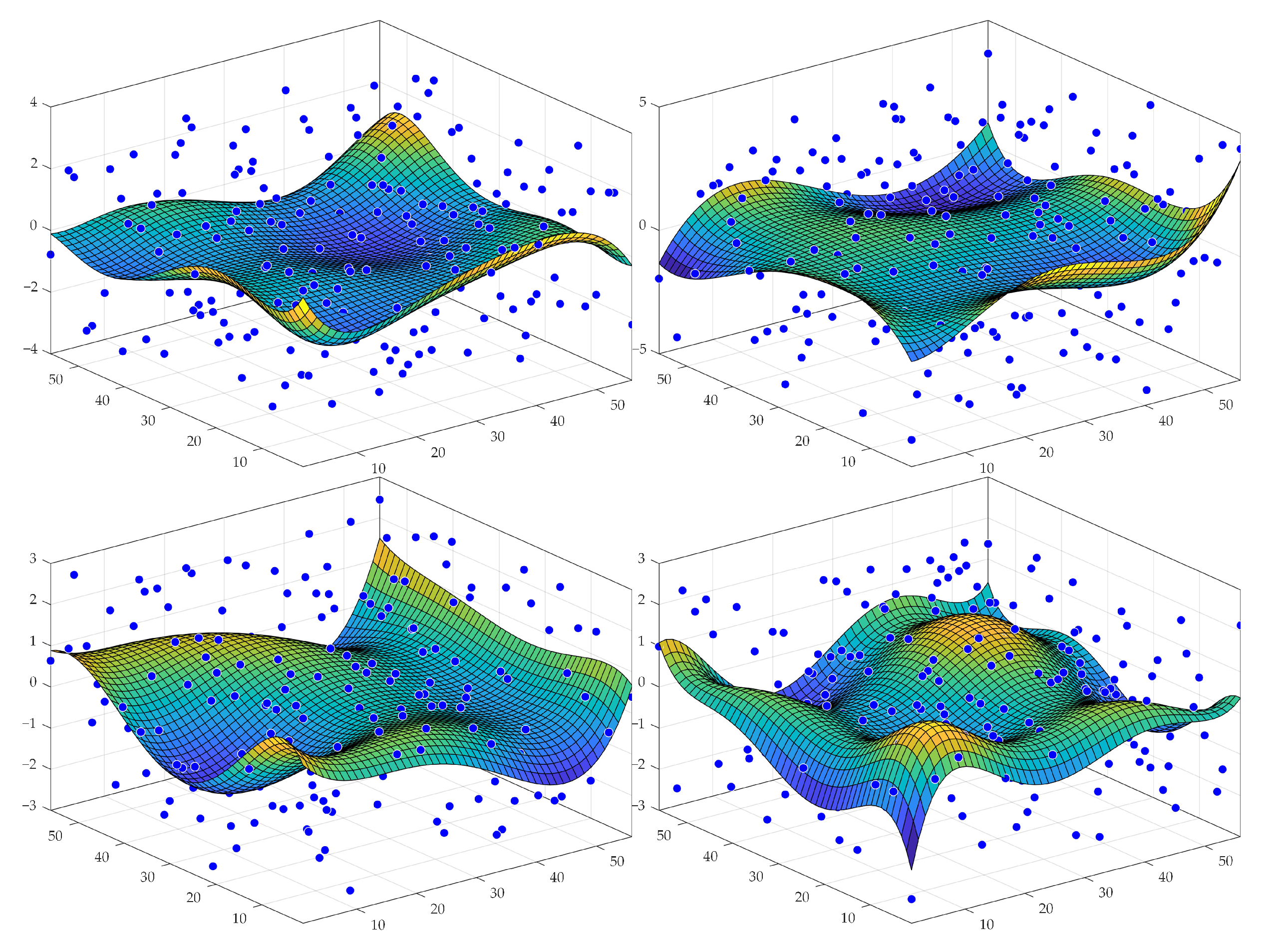
Initially, a set of background templates is created. Later, during the training of the ML model, background templates are randomly scaled (intensity scaling), providing the final varying background that is added to the synthetic protein spot image. The template of the varying background is created by fitting a polynomial surface of degree 5 in x and y directions. The polynomial surface is fitted to a randomly generated grid of points in a grid size of (in this case is the square patch size), and the values are drawn from the uniform distribution in the range . Later, the fitted surface is normalized by subtracting its mean and dividing by the largest value from the set of absolute values of the 5th and 95th percentiles. Samples of varying background templates are presented in Figure 5.
8. Add Gaussian noise. The high-frequency noise in real 2DGE images may be caused by staining non-protein substances in the gel, by gel damage, or by the imaging process. For transferring such distortions to the synthetic images, Gaussian noise is added. The noise is added to the entire region of the image sample. Gaussian noise is generated by randomly selecting variance from the range . The probability of adding noise to the image is . This task is implemented using the GaussNoise pixel-level transformation from the Albumentations library.
2.1.3. Generation of Protein Spot 2D Prototype (Primary Spot)
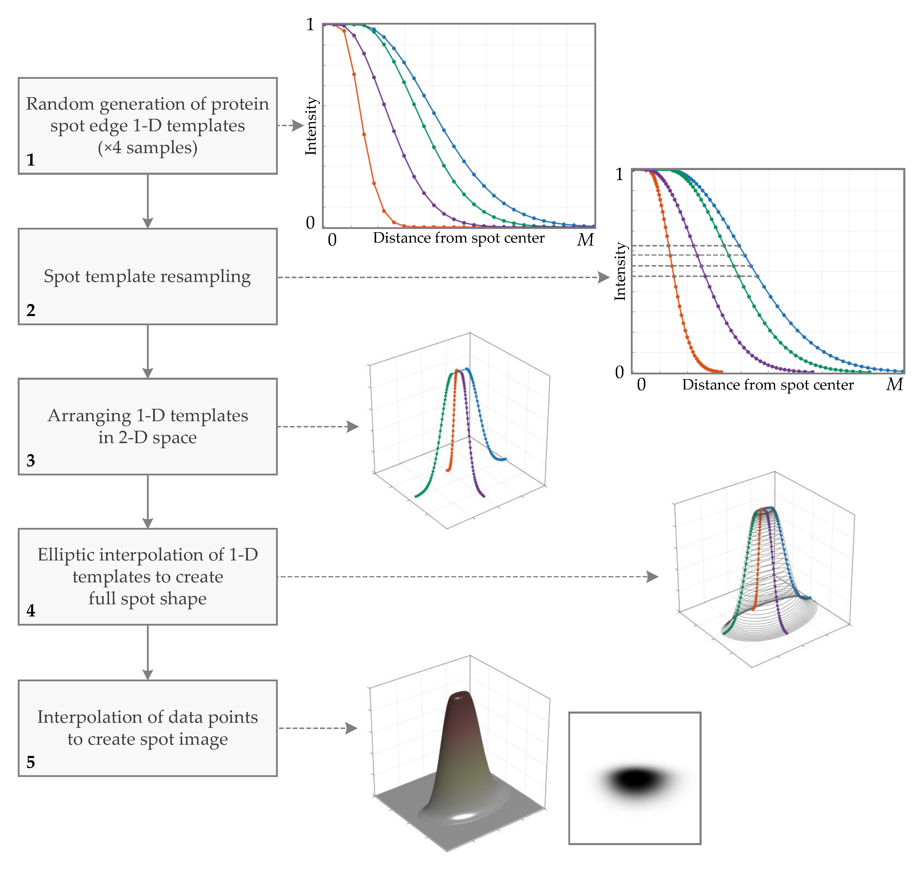
This is the first step of the main workflow of synthetic protein spot image generation. This step produces the initial appearance of the spot. In Section 2.1.1 and Figure 2, it was discussed that the fast approach of constructing the 2D shape of the spot from vertical and horizontal sections of the spot by vector outer product might lead to situations where the 2D shape of the spot starts to lose smoothness and appear cornered. Effects such as these start to show when generating more extremely saturated spots (spots with larger plateaus on the top). To overcome this problem, the 2D shape of the spot is inferred from the generated vertical and horizontal sections of the spot by elliptic interpolation.
The workflow of the prototype spot generation is as follows (Figure 4):
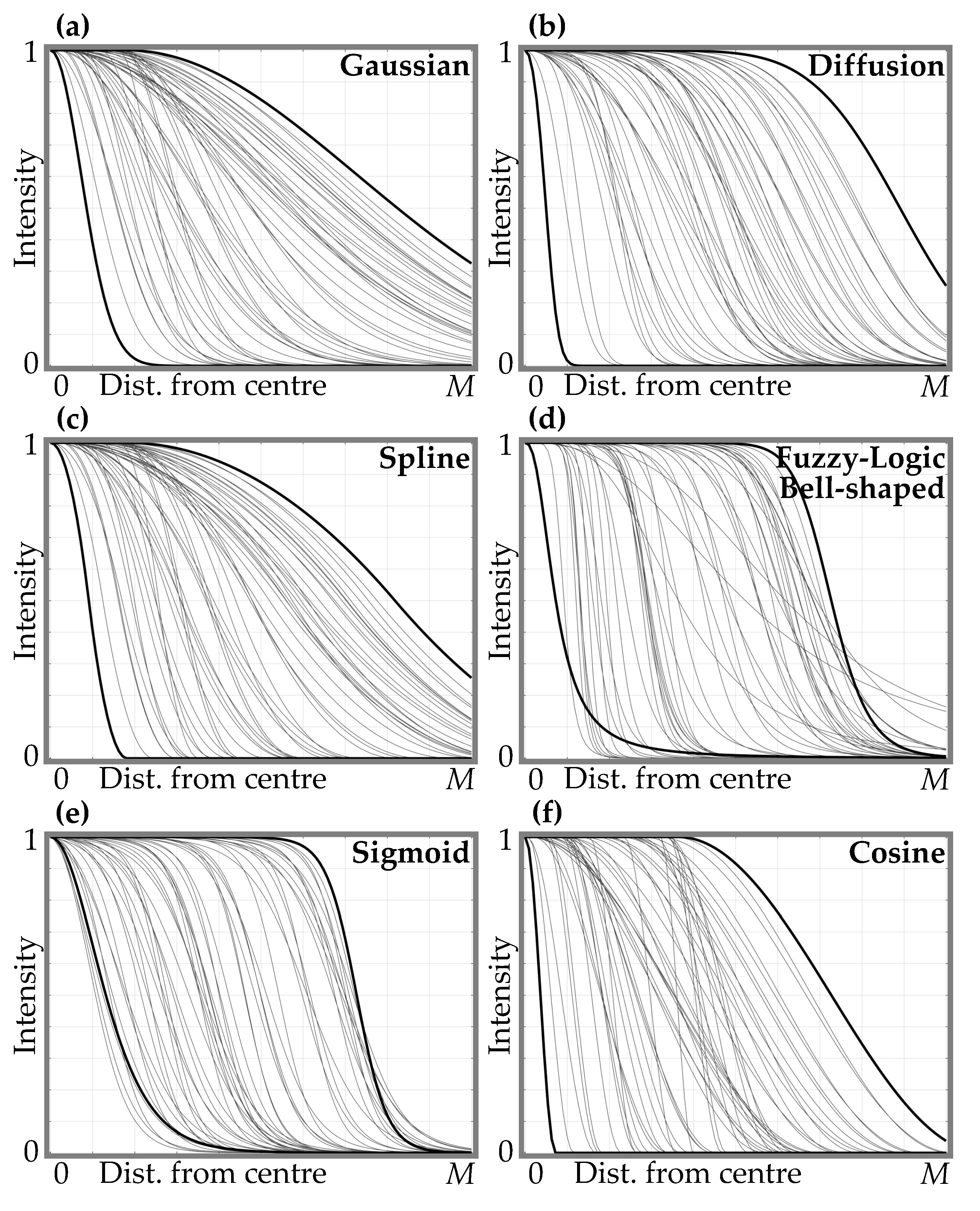
1. Random generation of protein spot edge 1D templates. The first step is to randomly select the mathematical function and its parameters that define the intensity profile of the spot sections. A single function serves as a protein spot edge 1D template. To generate a rich variety of spot shapes, the section of the spot is made of two 1D templates, and these templates are generated independently. For creating the spot, two sections (vertical and horizontal) are required, so four samples of templates must be created. Six functions are selected for the spot edge template generation: Gaussian, simplified diffusion process, spline, fuzzy logic generalized membership bell-shaped, sigmoid, and raised cosine. Mathematical functions are described further in this section, and their plots are shown in Figure 6.
2. Spot template resampling. To prepare templates for simple elliptic interpolation, the templates are resampled such that all templates have the same intensity values. Linear interpolation is used to solve the problem of finding x coordinates where the function acquires the required intensity values. The required intensity values are generated non-linearly dividing interval : the spacing of the samples at the ends of the interval is smaller than at the center to create a smoother template curve where the curvature is larger.
3. Arranging 1D templates in 2D space. The generated templates obtain their position in 2D space. Now each template defines a shape of the eastern, northern, western, and southern sides of the spot.
4. Elliptic interpolation of 1D templates to create the full spot shape. The arranged templates fill only parts of the spot at the cardinal axes (spot horizontal and vertical sections). This step performs the calculation of spot samples for the full area of the spot. Spot intensity values are acquired by elliptic interpolation of the template samples: an ellipse is fitted to the pair of samples that have the same value and belongs to the adjacent templates (the distances from the origin to the positions of the samples define the two axes of an ellipse); an ellipse is sampled at a range of angle values with a step of ; and x and y coordinates of the ellipse samples are collected to describe the shape of the spot. The elliptic interpolation is repeated for all template sample pairs in all quadrants.
5. Interpolation of data points to create the spot image. At this point, the computed samples that form the spot are irregularly scattered in 3D space (if point intensity is seen as z coordinate). In order to produce the 2D image of the spot, we need to resample the point cloud to obtain data points on the regular grid in the XY-plane. This is achieved by triangulation-based cubic interpolation for 2D cases. The final result is the image of the protein spot.
Protein Spot Edge Templates
Spot edge templates are needed to build vertical and horizontal sections of the protein spot. Edge templates are generated using mathematical functions (Equations (1)–(6)), which are described below. Plots of the functions are shown in Figure 6. Edge templates are generated by randomly selecting a function from the set of six functions (Equations (1)–(6)) and by randomly sampling parameters from the defined range (for parameter ranges, refer to Table 1).
Functions that determine the profile of the protein spot edge template:
- Gaussian function with its center at (the graph of the function is shown in Figure 6a):here d —shift of the mean of the Gaussian function from the spot center (); —standard deviation of the Gaussian function.
- Simplified diffusion process function with its center at (refer to Figure 6b):here ; D—parameter defining the diffusion (defines a slope and a shift from the center of the curve transition area); a is the radius of diffusion area.
- Spline function with its center at (refer to Figure 6c):here a is the distance from the center to the beginning of the curve transition area; b is the distance from the a to the end of the curve transition area.
- Fuzzy Logic generalized membership bell-shaped function with its center at (refer to Figure 6d):here a determines the width of the function’s transitional area; b defines the shape of the curve (slope) where a larger value gives a steeper function.
- Sigmoid function with its center at (Figure 6e):here a defines the slope of the transition area of the curve; d—distance from the center to the curve transition area.
- Raised cosine function with its center at (Figure 6f):here a is the width of the transition area of the curve; d—distance from the center to the curve transition area.
Function Parameter Ranges for Edge Template Generation
Table 1 summarizes the parameter value ranges used to generate 1D protein spot edge templates. The ranges of the parameters are adjusted for the generation of edge templates of length px (half of the image patch size, which is px in the current research).
2.2. Synthetic Data Evaluation
The created dataset must be evaluated in order to draw conclusions about its quality and potential for the development of ML models for protein spot reconstruction and parameterization.
Some initial subjective evaluations were performed during the process of creating the protein spot image samples. Subjective evaluation refers to the perceptual (visual) evaluation of the image samples’ fidelity to real 2DGE images. Subjective evaluation and domain knowledge were constantly used and exploited during the development of the method for generating synthetic protein spot images.
The objective evaluation of the dataset is possible after using the dataset for its intended purpose—to develop a spot modeling algorithm. If the dataset leads to the creation of an ML model that, according to relevant metrics, is appropriate for the protein spot modeling task (better than some previous models), the synthetic dataset can be treated as useful.
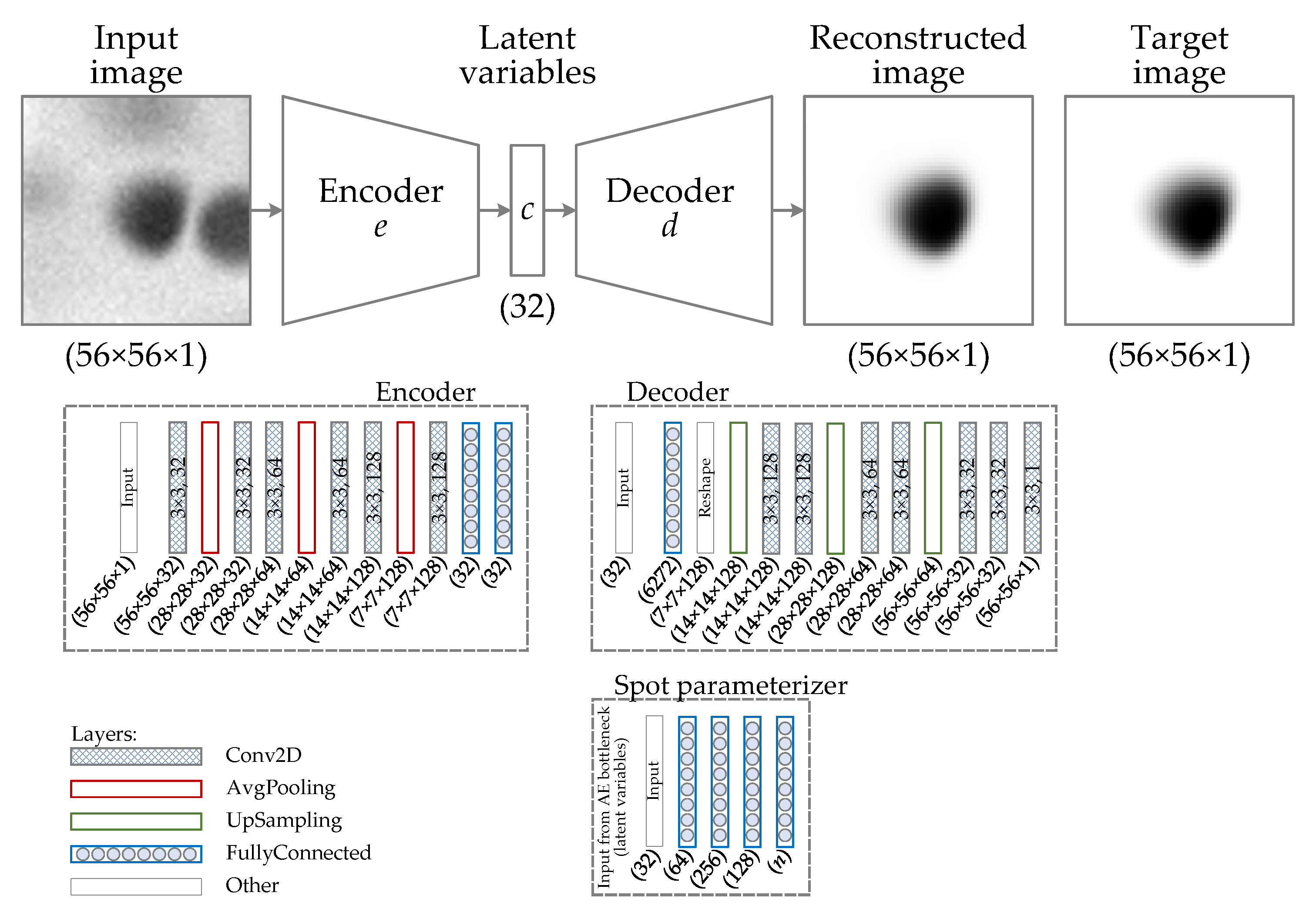
The machine learning approach is used for the development of the spot modeling algorithm. The autoencoder (AE) is selected to serve as the core part of the protein spot modeling/reconstruction algorithm. The architecture of the autoencoder, together with some of its hyperparameters, is presented in Figure 7. The AE model additionally has a branch for a second output for the prediction of spot parameters from the bottleneck features. This branch is a multilayer perceptron. The AE model is trained using a decreasing learning rate (LR) schedule. LR is linearly reduced from to over 60 epochs. The initial neural network’s architecture and hyperparameters are selected and tuned heuristically based on NN’s performance on validation data.
For the algorithm comparison, two models frequently used in the literature, namely the Gaussian [41,42,43,44,46] and diffusion [45,46] models for spot modeling, serve as baseline algorithms. Additionally, several other mathematical spot models [46] are used as baseline algorithms.
For the evaluation of the created spot reconstruction algorithm (autoencoder model), several comparative experiments are designed. There are two major groups of experiments: one comparison of the algorithms uses synthetic data that are similar to the training data, and the other is based on real 2DGE data. The advantage of synthetic data is the availability of precise ground-truth labels. Real data show algorithm performance in real-world scenarios. The performance results may differ from the synthetic data if not all variations of the real spots are represented in the synthetic data. The results of evaluations using the real data may be inaccurate due to the unknown real ground-truth data.
The other classes of experiments are the evaluation of the reconstruction accuracy and the evaluation of spot parameter estimation accuracy. The reconstruction accuracy reveals how similar the reconstructed spot is to the ground-truth spot. Parameter estimation accuracy shows how well the essential spot parameters—spot intensity (excluding background intensity) and spot volume—can be computed. Ground-truth spot parameters are computed directly from the synthetic target image. For the baseline algorithms (fitting mathematical model), the predicted spot parameters are computed from the estimated model parameters and from the fitted model. For the AE-based reconstruction algorithm, indirectly predicted spot parameters are computed from the reconstructed spot, and directly predicted parameters are from the bottleneck features.
As the synthetic dataset holds information about spot background intensity, the AE can be trained to reconstruct the spot in two modes—either removing or leaving the background. Both cases are evaluated for reconstruction and for spot parameter prediction.
The evaluation of spot modeling is based on the following metrics: the normalized sum of squared error (NSSE) (Equation (7)) for the spot reconstruction evaluation and the normalized mean of squared error (NMSE) for the spot parameter estimation. NMSE is MSE normalized by the variance of ground-truth parameters.
During the modeling of protein spots (fitting baseline mathematical models), a patch of a 2DGE image is approximated by a mathematical model. For the constrained minimization problem, the Matlab implementation of the Trust-region-reflective least-squares algorithm [52,53] is used, which seeks to minimize the sum of squared residuals. For the evaluation of the spot modeling, the normalized sum of squared residuals is used as a metric and is defined by the function:
here —2DGE image patch containing the protein spot being modeled; —the ground-truth (target) image patch; —the number of points in the modeled region of the 2DGE image; and —the background and the peak intensity values of the ground-truth spot, respectively.
2.3. Software Used
The software tools and programming languages used in this research are as follows:
- MATLAB programming and numeric computing platform (version R2021a, The Mathworks Inc., Natick, MA, USA) for the implementation of mathematical protein spot models, for offline data generation of synthetic dataset creation workflow, and for data analysis and visualization;
- Python (version 3.9.10) (https://www.python.org), (accessed on 1 February 2022) [54], an interpreted, high-level, general-purpose programming language. Used for the synthetic dataset creation workflow and for machine learning applications;
- TensorFlow with Keras (version 2.6.0) (https://www.tensorflow.org, (accessed on 1 February 2022)) [55], an open-source platform for machine learning. Used for the online data augmentation stage of the synthetic dataset creation workflow and for the training of autoencoders;
- Albumentations (version 1.0.3) (https://albumentations.ai, (accessed on 1 February 2022)) [50], a Python library for fast and flexible image augmentation. Used for the synthetic dataset creation workflow;
- OpenCV (version 4.5.1) (https://opencv.org/, (accessed on 1 February 2022)) [56], an open source computer vision library. Used for image input/output and manipulations.
2.4. Data Collection
For the experimental evaluation of the proposed method for generating synthetic high-fidelity 2DGE image patches, the synthetic dataset is prepared and used for the development of the ML-based protein spot reconstruction algorithm. The trained model is evaluated using simulated test data and collected real spot data:
- Synthetic data: the created synthetic test set of spot images is fully and openly available. It can be found at Mendeley Data (https://doi.org/10.17632/x62kt53nnr.1), (accessed on 25 April 2022) The test set consists of 40,000 samples. The training set is not shared online due to its size, but it is similar to the test set as both sets were generated using the same method.
- Real test data: a test set of spots is compiled from real 2DGE images. Spots in images are detected and segmented using the method described in [46,57]. The minimum size of the cropped image patches is px. Crop boxes are centered at the spot centers. The crop box must fully contain the region of the spot that is defined by the mask image. If necessary, the crop box is expanded to fully include the spot region. The test set consists of 6725 samples. 2DGE images were obtained from the following databases or other types of sources:
- -
- Proteome 2D-PAGE Database (https://protein.mpiib-berlin.mpg.de/cgi-bin/pdbs/2d-page/extern/index.cgi), (accessed on 21 February 2022) [58];
- -
- The LECB 2-D PAGE Gel Images Data Sets (http://bioinformatics.org/lecb2dgeldb/), (accessed on 21 February 2022);
- -
- The Human Myocardial Two-Dimensional Electrophoresis Protein Database (HEART-2DPAGE) (http://www.chemie.fu-berlin.de/user/pleiss/), (accessed on 21 February 2022) [59];
- -
- HeLa Study Reference Images (http://www.fixingproteomics.org/advice/helastandard.html), (accessed on 11 August 2010) [60,61];
- -
- Images used in the validation of RAIN algorithm [62] (http://www.proteomegrid.org/rain/, (accessed on 20 July 2009)).
3. Results and Discussion
This work presents and evaluates a method for the creation of a synthetic dataset of 2DGE image patches that are needed for the development of 2DGE protein spot modeling and reconstruction algorithms.
The generation of realistic synthetic datasets is becoming an increasingly important task in the field of machine learning (ML). Real data are costly to acquire. There are situations when real data are very scarce, rare, or hard to acquire and use due to privacy issues. The important property of synthetic datasets is that accurate ground-truth labels are available inherently, so it costs nothing to generate labels once the appropriate input images are generated. The increasing capability of generating realistic synthetic data boosts the performance of ML models. The use of purely synthetic data, or a mix of real and synthetic data, is gaining traction, and it is predicted that such uses will overtake the usage of datasets containing only real data.
The developed algorithm for protein spot reconstruction, modeling, and parameterization is evaluated in two major aspects. The first is the reconstruction performance of the synthetic and real 2DGE spot data (Figure 8). The second is the estimation accuracy of the spot key parameters (peak intensity and integrated spot intensity (volume)) (Figure 9). The terms “reconstruction”, “modeling”, and “parameterization” can be interpreted as follows: reconstruction—the algorithm reconstructs the spot without noise; modeling—the AE algorithm creates an internal representation of the spot (features from the bottleneck layer), and the spot image can be generated from these features; parameterization—the algorithm can predict parameters of the protein spot.
To acquire a better view of the algorithm’s performance in different situations when dealing with spot image distortions, several experimental setups are prepared. Thus, the new and baseline algorithms for spot modeling are tested in the following situations.
Conducted spot reconstruction experiments (Figure 8):
- Reconstruction of synthetic images:
- -
- input image may contain only the primary spot or the primary spot surrounded by secondary spots. These cases are marked by “=1spot” or “>1spot”, respectively, in the graphs of Figure 8a;
- -
- during the model fitting and the evaluation of reconstruction residual error, the mask of the primary spot may or may not be used. The baseline algorithms use a mask to fit a model only in the mask area. AE does not use the mask as additional input data. All algorithms use the mask for residual error evaluation if the mask is provided in a particular experiment. These cases are marked by “+Mask” or “−Mask”, respectively, in the graphs of Figure 8a;
- -
- input images may be corrupted by Gaussian noise (marked by “+Noise”), by slowly varying background (marked by “+Bckg”), or neither (no additional marking);
- -
- two AE models are trained and evaluated—”AE−B” is the model that reconstructs the image with background eliminated and “AE−B” reconstructs the image with the constant background.
- Reconstruction of real images:
- -
- due to the fact that in real 2DGE images the ground-truth spots are unknown, the experimental setup is slightly different. The ground-truth images are simulated, in one experimental case, by smoothing original spot images using a median filter (marked by “−Noise” in Figure 8b). In the other case, the ground-truth images are the same, but the input images are generated by adding Gaussian and Salt & Pepper noise to the ground-truth images (noted by “+Noise” in the legend);
- -
- during the fitting of the baseline models, the mask of the main spot may or may not be used. The mask is always used when evaluating residual errors. Cases are marked by “+Mask” or “−Mask”, respectively, in the graphs of Figure 8b;
- -
- the true background intensity is difficult to estimate, so the AE was used to reconstruct spots with the background (“AE+B” algorithm).
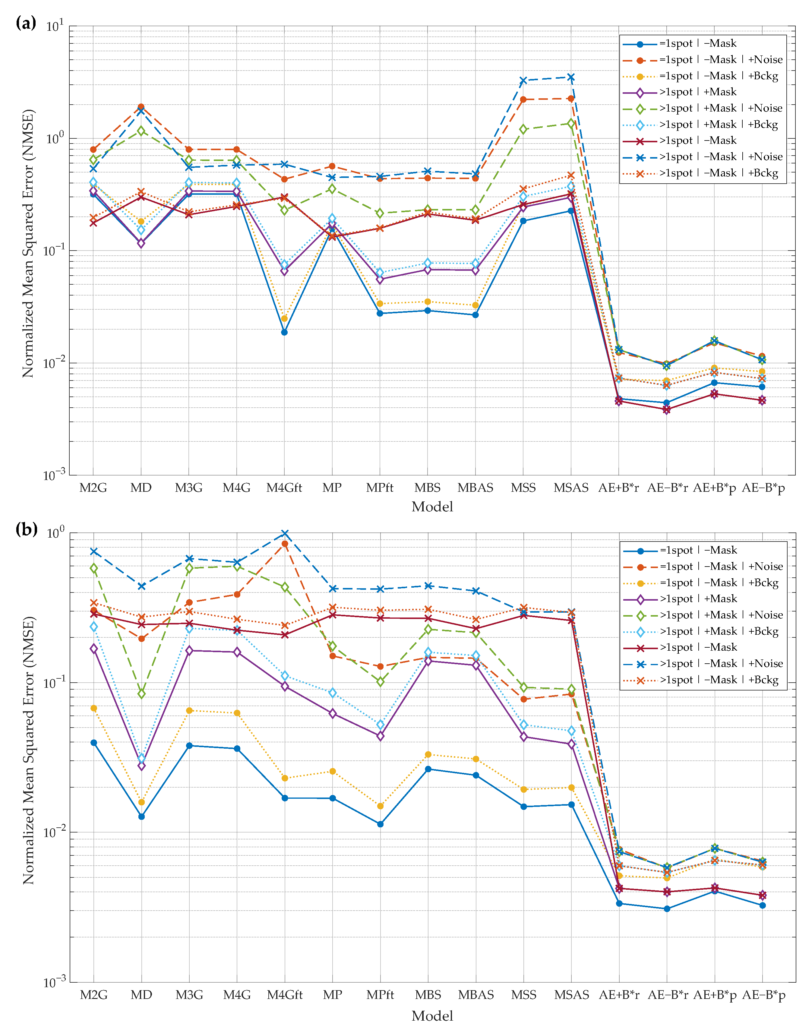
The results of the spot parameter estimation experiments are presented in (Figure 9). This experiment is performed using the synthetic images only due to the fact that the ground-truth parameters of the real spots are unknown. The experimental cases are the same as in the reconstruction of the synthetic images: “=1spot” or “>1spot”; “+Mask” or “−Mask”; and “+Noise”, “+Bckg”, or neither. Spot parameters can be computed in two ways: from the reconstructed spot or predicted from the bottleneck features of the AE. Both solutions are implemented and experimentally compared. Algorithms “AE+B*r” and “AE−B*r” compute the spot’s parameters from the reconstructed spot. Algorithms “AE+B*p” and “AE−B*p” predict the spot’s parameters from the AE’s bottleneck features.
The following is a list of the protein spot baseline models evaluated and compared during the experiments [42,45,46,63]:
- Two-way adapting (anisotropic) 2D Gaussian model (M2G);
- The diffusion model (MD);
- Three Gaussian functions model (M3G);
- Four Gaussian functions model (M4G);
- Four Gaussian functions with flat top model (M4GFT);
- Simple -shaped model (MP);
- -shape model with flat top (MPft);
- Two-way symmetric bell-shaped model (MBS);
- Asymmetric bell-shaped model (MBAS);
- Two-way symmetric sigmoid-based model (MSS);
- Asymmetric sigmoid-based model (MSAS).
The following is a list of the new spot reconstruction algorithm variants or the separate outputs of the same algorithm that were included in the evaluation results (graphs):
- “AE+B”—spot reconstructed by the autoencoder with the constant background remaining;
- “AE−B”—spot reconstructed by the autoencoder without background;
- “AE+B*r”—spot parameters computed from the reconstructed spot, and background is not removed during reconstruction;
- “AE−B*r”—spot parameters computed from the reconstructed spot, and background is removed during reconstruction;
- “AE+B*p”—spot parameters predicted from the AE’s bottleneck features, and AE is trained to reconstruct the spot leaving the background;
- “AE−B*p”—spot parameters predicted from the AE’s bottleneck features, and AE is trained to reconstruct the spot without background.
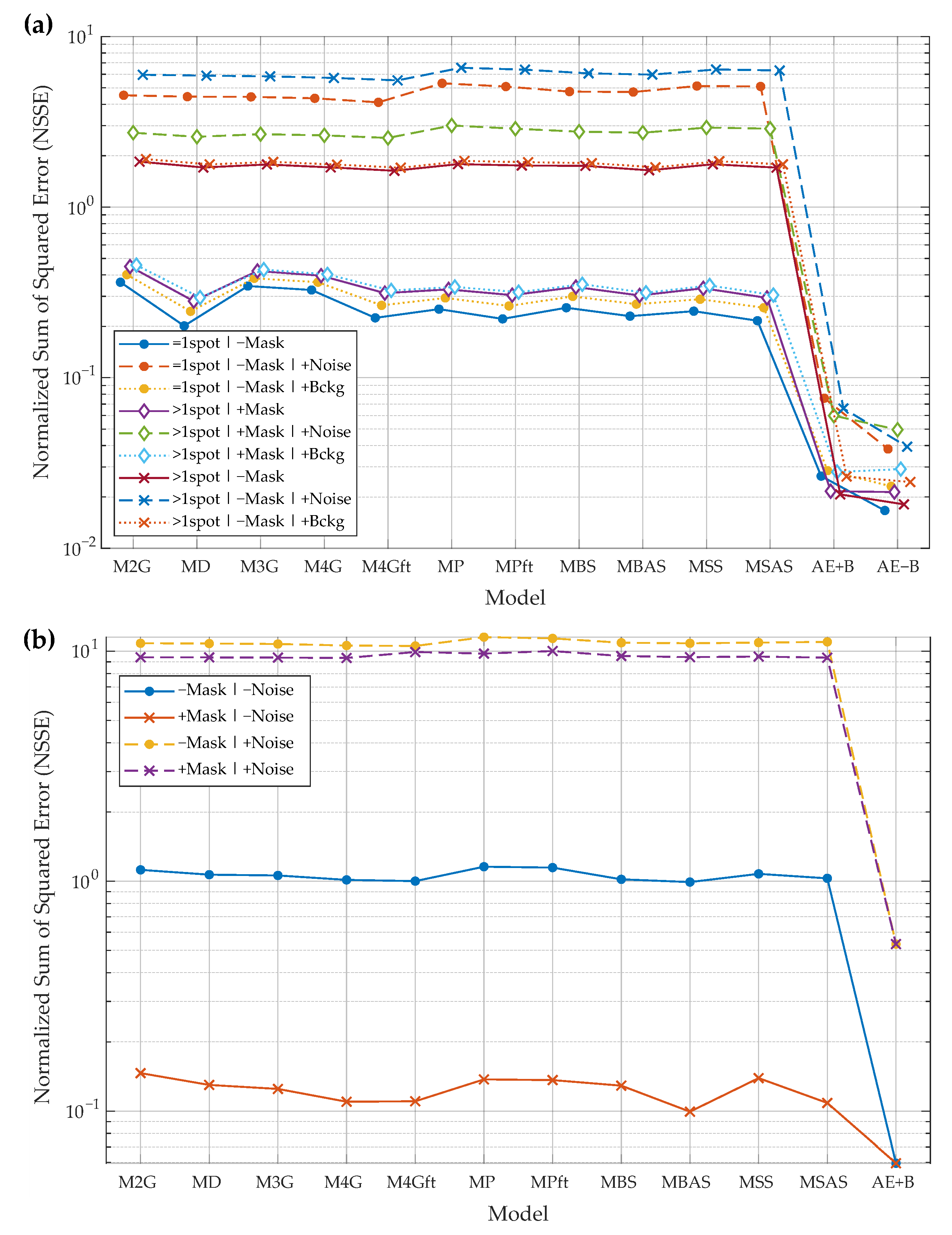
To summarize the results of all the experiments, the developed spot reconstruction algorithm trained using only synthetic data outperforms all the baseline algorithms in all experiments based on synthetic and real data. Lower performance gains are achieved when the experimental data includes the least noise. When additional noise is introduced, the new algorithm performs better with a larger margin, and this tendency holds in all cases. The advantage of the new algorithm is that it works without the initial mask of the main protein spot, so it is not influenced by possible mask errors. Baseline algorithms require the mask of the main spot in order to perform better; experiments where the mask is used or not show that the baseline algorithms depend on the mask, so errors in mask extraction influence the results of the baseline algorithms.
Spot parameter prediction experiments reveal that the new algorithms that are trained to remove background perform slightly better than the algorithm trained to leave background. The same tendency is observable in the spot reconstruction experiments. Spot parameter prediction from the bottleneck features performs almost equally with parameter estimation from the reconstructed spot. As such, the Decoder part of AE may be dropped in favor of using only the small multilayer perceptron, which predicts spot parameters from the bottleneck features. If only the spot parameters and not the reconstructed spot are needed, the computational load may be decreased.
The proposed synthetic image generation method is useful in developing protein spot reconstruction models. The method can be easily adapted to similar tasks where image analysis tools are required to process circular, blob-type patterns in images.
4. Conclusions
This work proposes a method for the generation of synthetic 2DGE image samples. A dataset of simulated 2DGE image patches is used for the development of a 2DGE protein spot modeling and reconstruction algorithm.
The developed protein spot reconstruction algorithm was tested using synthetic and real data. The evaluation of the spot reconstruction algorithm serves as a proxy for the evaluation of the synthetic data generation method. Evaluation results show that the created synthetic dataset is useful for the development of protein spot models. The developed algorithm outperformed all the baseline algorithms in all experimental cases.
Synthetic data allowed the training of an ML model-based spot reconstruction algorithm that performs well on real data. The usage of synthetic data in the development of ML models is becoming more widespread. Synthetic data generation allows the creation of samples of rare cases, the construction of diverse datasets, and the training of more accurate ML models.
Funding
This research received no external funding.
Institutional Review Board Statement
Not applicable.
Informed Consent Statement
Not applicable.
Data Availability Statement
The created synthetic test set is openly available and can be found at Mendeley Data (https://doi.org/10.17632/x62kt53nnr.1), (accessed on 25 April 2022). For other 3rd party two-dimensional electrophoresis gel images please refer to Section 2.4.
Conflicts of Interest
The author declares no conflict of interest.
Abbreviations
The following abbreviations are used in this manuscript:
| 2DGE, 2DE | Two-dimensional Gel Electrophoresis |
| ML | Machine Learning |
| AI | Artificial Intelligence |
| AE | Autoencoder |
| ANN | Artificial Neural Network |
| CNN | Convolutional Neural Network |
| LR | Learning Rate |
| MSE | Mean Squared Error |
| NMSE | Normalized Mean Squared Error |
| SSE | Sum of Squared Error |
| NSSE | Normalized Sum of Squared Error |
References
- O’Farrell, P. High Resolution 2-Dimensional Electrophoresis of Proteins. J. Biol. Chem. 1975, 250, 4007–4021. [Google Scholar] [CrossRef]
- Moche, M.; Albrecht, D.; Maaß, S.; Hecker, M.; Westermeier, R.; Büttner, K. The new horizon in 2D electrophoresis: New technology to increase resolution and sensitivity. Electrophoresis 2013, 34, 1510–1518. [Google Scholar] [CrossRef] [PubMed]
- Koo, H.N.; Seok, S.J.; Kim, H.K.; Kim, G.H.; Yang, J.O. Comparative Proteomics Analysis of Phosphine-Resistant and Phosphine-Susceptible Sitophilus oryzae (Coleoptera: Curculionidae). Appl. Sci. 2021, 11, 4163. [Google Scholar] [CrossRef]
- Venugopal, D.C.; Ravindran, S.; Shyamsundar, V.; Sankarapandian, S.; Krishnamurthy, A.; Sivagnanam, A.; Madhavan, Y.; Ramshankar, V. Integrated Proteomics Based on 2D Gel Electrophoresis and Mass Spectrometry with Validations: Identification of a Biomarker Compendium for Oral Submucous Fibrosis—An Indian Study. J. Pers. Med. 2022, 12, 208. [Google Scholar] [CrossRef]
- Guzmán-Flores, J.M.; Flores-Pérez, E.C.; Hernández-Ortiz, M.; Vargas-Ortiz, K.; Ramírez-Emiliano, J.; Encarnación-Guevara, S.; Pérez-Vázquez, V. Protein expression profile of twenty-week-old diabetic db/db and non-diabetic mice livers: A proteomic and bioinformatic analysis. Biomolecules 2018, 8, 35. [Google Scholar] [CrossRef] [Green Version]
- Ura, B.; Biffi, S.; Monasta, L.; Arrigoni, G.; Battisti, I.; Di Lorenzo, G.; Romano, F.; Aloisio, M.; Celsi, F.; Addobbati, R.; et al. Two Dimensional-Difference in Gel Electrophoresis (2D-DIGE) Proteomic Approach for the Identification of Biomarkers in Endometrial Cancer Serum. Cancers 2021, 13, 3639. [Google Scholar] [CrossRef]
- Rogowska-Wrzesinska, A.; Le Bihan, M.C.; Thaysen-Andersen, M.; Roepstorff, P. 2D gels still have a niche in proteomics. J. Proteom. 2013, 88, 4–13. [Google Scholar] [CrossRef]
- Oliveira, B.M.; Coorssen, J.R.; Martins-de Souza, D. 2DE: The Phoenix of Proteomics. J. Proteom. 2014, 104, 140–150. [Google Scholar] [CrossRef]
- Abdallah, C.; Dumas-Gaudot, E.; Renaut, J.; Sergeant, K. Gel-based and gel-free quantitative proteomics approaches at a glance. Int. J. Plant Genom. 2012, 2012. [Google Scholar] [CrossRef] [Green Version]
- Kim, Y.I.; Cho, J.Y. Gel-based proteomics in disease research: Is it still valuable? Biochim. Biophys. Acta (BBA)-Proteins Proteom. 2019, 1867, 9–16. [Google Scholar] [CrossRef]
- Bocian, A.; Buczkowicz, J.; Jaromin, M.; Hus, K.K.; Legáth, J. An effective method of isolating honey proteins. Molecules 2019, 24, 2399. [Google Scholar] [CrossRef] [PubMed] [Green Version]
- Rabilloud, T.; Chevallet, M.; Luche, S.; Lelong, C. Two-dimensional gel electrophoresis in proteomics: Past, present and future. J. Proteom. 2010, 73, 2064–2077. [Google Scholar] [CrossRef] [PubMed] [Green Version]
- Lee, P.Y.; Saraygord-Afshari, N.; Low, T.Y. The evolution of two-dimensional gel electrophoresis-from proteomics to emerging alternative applications. J. Chromatogr. A 2020, 1615, 460763. [Google Scholar] [CrossRef] [PubMed]
- Fulton, K.M.; Twine, S.M. Immunoproteomics: Current technology and applications. In Immunoproteomics; Springer: Berlin/Heidelberg, Germany, 2013; pp. 21–57. [Google Scholar]
- Leber, T.M.; Balkwill, F.R. Zymography: A single-step staining method for quantitation of proteolytic activity on substrate gels. Anal. Biochem. 1997, 249, 24–28. [Google Scholar] [CrossRef] [PubMed]
- Lee, B.S.; Jayathilaka, L.P.; Huang, J.S.; Gupta, S. Applications of immobilized metal affinity electrophoresis. In Electrophoretic Separation of Proteins; Springer: Berlin/Heidelberg, Germany, 2019; pp. 371–385. [Google Scholar]
- Werhahn, W.; Braun, H.P. Biochemical dissection of the mitochondrial proteome from Arabidopsis thaliana by three-dimensional gel electrophoresis. Electrophoresis 2002, 23, 640–646. [Google Scholar] [CrossRef]
- Valledor, L.; Jorrín, J. Back to the basics: Maximizing the information obtained by quantitative two dimensional gel electrophoresis analyses by an appropriate experimental design and statistical analyses. J. Proteom. 2011, 74, 1–18. [Google Scholar] [CrossRef]
- Schnaars, V.; Dörries, M.; Hutchins, M.; Wöhlbrand, L.; Rabus, R. What’s the Difference? 2D DIGE Image Analysis by DeCyderTM versus SameSpotsTM. J. Mol. Microbiol. Biotechnol. 2018, 28, 128–136. [Google Scholar] [CrossRef]
- Jungblut, P.R. The proteomics quantification dilemma. J. Proteom. 2014, 107, 98–102. [Google Scholar] [CrossRef]
- Brandão, A.; Barbosa, H.; Arruda, M. Image analysis of two-dimensional gel electrophoresis for comparative proteomics of transgenic and non-transgenic soybean seeds. J. Proteom. 2010, 73, 1433–1440. [Google Scholar] [CrossRef]
- Molina-Mora, J.A.; Chinchilla-Montero, D.; Castro-Peña, C.; García, F. Two-dimensional gel electrophoresis (2D-GE) image analysis based on CellProfiler: Pseudomonas aeruginosa AG1 as model. Medicine 2020, 99, e23373. [Google Scholar] [CrossRef]
- Dowsey, A.W.; English, J.A.; Lisacek, F.; Morris, J.S.; Yang, G.Z.; Dunn, M.J. Image analysis tools and emerging algorithms for expression proteomics. Proteomics 2010, 10, 4226–4257. [Google Scholar] [CrossRef] [PubMed] [Green Version]
- Natale, M.; Maresca, B.; Abrescia, P.; Bucci, E. Image analysis workflow for 2-D electrophoresis gels based on ImageJ. Proteom. Insights 2011, 4, 37–49. [Google Scholar] [CrossRef] [Green Version]
- Morris, J.S.; Clark, B.N.; Wei, W.; Gutstein, H.B. Evaluating the performance of new approaches to spot quantification and differential expression in 2-dimensional gel electrophoresis studies. J. Proteome Res. 2009, 9, 595–604. [Google Scholar] [CrossRef] [PubMed] [Green Version]
- Berth, M.; Moser, F.M.; Kolbe, M.; Bernhardt, J. The state of the art in the analysis of two-dimensional gel electrophoresis images. Appl. Microbiol. Biotechnol. 2007, 76, 1223–1243. [Google Scholar] [CrossRef] [PubMed] [Green Version]
- Srinark, T.; Kambhamettu, C. An image analysis suite for spot detection and spot matching in two-dimensional electrophoresis gels. Electrophoresis 2008, 29, 706–715. [Google Scholar] [CrossRef]
- Brauner, J.M.; Groemer, T.W.; Stroebel, A.; Grosse-Holz, S.; Oberstein, T.; Wiltfang, J.; Kornhuber, J.; Maler, J.M. Spot quantification in two dimensional gel electrophoresis image analysis: Comparison of different approaches and presentation of a novel compound fitting algorithm. BMC Bioinform. 2014, 15, 181. [Google Scholar] [CrossRef] [Green Version]
- Li, F.; Seillier-Moiseiwitsch, F.; Korostyshevskiy, V.R. Region-based statistical analysis of 2D PAGE images. Comput. Stat. Data Anal. 2011, 55, 3059–3072. [Google Scholar] [CrossRef] [Green Version]
- Millioni, R.; Puricelli, L.; Sbrignadello, S.; Iori, E.; Murphy, E.; Tessari, P. Operator-and software-related post-experimental variability and source of error in 2-DE analysis. Amino Acids 2012, 42, 1583–1590. [Google Scholar] [CrossRef]
- Kostopoulou, E.; Katsigiannis, S.; Maroulis, D. SpotDSQ: A 2D-gel image analysis tool for protein spot detection, segmentation and quantification. In Proceedings of the 2019 IEEE 19th International Conference on Bioinformatics and Bioengineering (BIBE), Athens, Greece, 28–30 October 2019; pp. 31–37. [Google Scholar]
- Goez, M.M.; Torres-Madronero, M.C.; Rothlisberger, S.; Delgado-Trejos, E. Joint pre-processing framework for two-dimensional gel electrophoresis images based on nonlinear filtering, background correction and normalization techniques. BMC Bioinform. 2020, 21, 376. [Google Scholar] [CrossRef]
- Sengar, R.S.; Upadhyay, A.K.; Singh, M.; Gadre, V.M. Analysis of 2D-gel images for detection of protein spots using a novel non-separable wavelet based method. Biomed. Signal Process. Control. 2016, 25, 62–75. [Google Scholar] [CrossRef]
- Nhek, S.; Tessema, B.; Indahl, U.; Martens, H.; Mosleth, E. 2D electrophoresis image segmentation within a pixel-based framework. Chemom. Intell. Lab. Syst. 2015, 141, 33–46. [Google Scholar] [CrossRef]
- Shamekhi, S.; Baygi, M.H.M.; Azarian, B.; Gooya, A. A novel multi-scale Hessian based spot enhancement filter for two dimensional gel electrophoresis images. Comput. Biol. Med. 2015, 66, 154–169. [Google Scholar] [CrossRef] [PubMed]
- Kostopoulou, E.; Zacharia, E.; Maroulis, D. An Effective Approach for Detection and Segmentation of Protein Spots on 2-D Gel Images. IEEE J. Biomed. Health Inform. 2014, 18, 67–76. [Google Scholar] [CrossRef] [PubMed]
- dos Anjos, A.; Møller, A.L.; Ersbøll, B.K.; Finnie, C.; Shahbazkia, H.R. New approach for segmentation and quantification of two-dimensional gel electrophoresis images. Bioinformatics 2011, 27, 368–375. [Google Scholar] [CrossRef] [Green Version]
- Morris, J.S.; Clark, B.N.; Gutstein, H.B. Pinnacle: A fast, automatic and accurate method for detecting and quantifying protein spots in 2-dimensional gel electrophoresis data. Bioinformatics 2008, 24, 529–536. [Google Scholar] [CrossRef] [Green Version]
- Kostopoulou, E.; Katsigiannis, S.; Maroulis, D. 2D-gel spot detection and segmentation based on modified image-aware grow-cut and regional intensity information. Comput. Methods Programs Biomed. 2015, 122, 26–39. [Google Scholar] [CrossRef] [PubMed]
- Fernandez-Lozano, C.; Seoane, J.A.; Gestal, M.; Gaunt, T.R.; Dorado, J.; Pazos, A.; Campbell, C. Texture analysis in gel electrophoresis images using an integrative kernel-based approach. Sci. Rep. 2016, 6, 19256. [Google Scholar] [CrossRef] [Green Version]
- Goez, M.M.; Torres-Madroñero, M.C.; Röthlisberger, S.; Delgado-Trejos, E. Preprocessing of 2-dimensional gel electrophoresis images applied to proteomic analysis: A review. Genom. Proteom. Bioinform. 2018, 16, 63–72. [Google Scholar] [CrossRef]
- Garrels, J.I. The QUEST system for quantitative analysis of two-dimensional gels. J. Biol. Chem. 1989, 264, 5269–5282. [Google Scholar] [CrossRef]
- Marczyk, M. Mixture Modeling of 2-D Gel Electrophoresis Spots Enhances the Performance of Spot Detection. IEEE Trans. Nanobiosci. 2017, 16, 91–99. [Google Scholar] [CrossRef]
- Rogers, M.; Graham, J.; Tonge, P. Using statistical image models for objective evaluation of spot detection in two-dimensional gels. Proteomics 2003, 3, 879–886. [Google Scholar] [CrossRef]
- Bettens, E.; Scheunders, P.; Vandyck, D.; Moens, L.; Vanosta, P. Computer analysis of two-dimensional electrophoresis gels: A new segmentation and modeling algorithm. Electrophoresis 1997, 18, 792–798. [Google Scholar] [CrossRef] [PubMed]
- Navakauskienė, R.; Navakauskas, D.; Borutinskaitė, V.; Matuzevičius, D. Computational Methods for Proteome Analysis. In Epigenetics and Proteomics of Leukemia: A Synergy of Experimental Biology and Computational Informatics; Springer International Publishing: Cham, Switzerland, 2021; pp. 195–282. [Google Scholar] [CrossRef]
- Serackis, A.; Navakauskas, D. Treatment of over-saturated protein spots in two-dimensional electrophoresis gel images. Informatica 2010, 21, 409–424. [Google Scholar] [CrossRef]
- Ahmed, A.S.; El-Behaidy, W.H.; Youssif, A.A. Medical image denoising system based on stacked convolutional autoencoder for enhancing 2-dimensional gel electrophoresis noise reduction. Biomed. Signal Process. Control 2021, 69, 102842. [Google Scholar] [CrossRef]
- NVIDIA. What Is Synthetic Data. Available online: https://blogs.nvidia.com/blog/2021/06/08/what-is-synthetic-data/ (accessed on 14 March 2022).
- Buslaev, A.; Iglovikov, V.I.; Khvedchenya, E.; Parinov, A.; Druzhinin, M.; Kalinin, A.A. Albumentations: Fast and Flexible Image Augmentations. Information 2020, 11, 125. [Google Scholar] [CrossRef] [Green Version]
- Vincent, L.; Soille, P. Watersheds in Digital Spaces—An Efficient Algorithm Based on Immersion Simulations. IEEE Trans. Pattern Anal. Mach. Intell. 1991, 13, 583–598. [Google Scholar] [CrossRef] [Green Version]
- Coleman, T.F.; Li, Y. An interior trust region approach for nonlinear minimization subject to bounds. Siam J. Optim. 1996, 6, 418–445. [Google Scholar] [CrossRef] [Green Version]
- Coleman, T.; Li, Y. On the convergence of reflective newton methods for large-scale nonlinear minimization subject to bounds. Math. Program. 1994, 67, 189–224. [Google Scholar] [CrossRef]
- Van Rossum, G.; Drake, F.L. Python 3 Reference Manual; CreateSpace: Scotts Valley, CA, USA, 2009. [Google Scholar]
- Abadi, M.; Agarwal, A.; Barham, P.; Brevdo, E.; Chen, Z.; Citro, C.; Corrado, G.S.; Davis, A.; Dean, J.; Devin, M.; et al. TensorFlow: Large-Scale Machine Learning on Heterogeneous Systems. 2015. Available online: https://www.tensorflow.org (accessed on 1 February 2022).
- Bradski, G. The OpenCV Library. Dr. Dobb’s J. Softw. Tools 2000, 25, 120–123. [Google Scholar]
- Matuzevičius, D.; Žurauskas, E.; Navakauskienė, R.; Navakauskas, D. Improved proteomic characterization of human myocardium and heart conduction system by computational methods. Biologija 2008, 54, 283–289. [Google Scholar] [CrossRef] [Green Version]
- Lange, S.; Rosenkrands, I.; Stein, R.; Andersen, P.; Kaufmann, S.H.; Jungblut, P.R. Analysis of protein species differentiation among mycobacterial low-Mr-secreted proteins by narrow pH range Immobiline gel 2-DE-MALDI-MS. J. Proteom. 2014, 97, 235–244. [Google Scholar] [CrossRef] [PubMed]
- Plei, K.P.; Söding, P.; Sander, S.; Oswald, H.; Neuß, M.; Regitz-Zagrosek, V.; Fleck, E. Dilated cardiomyopathy-associated proteins and their presentation in a WWW-accessible two-dimensional gel protein database. Electrophoresis 1997, 18, 802–808. [Google Scholar] [CrossRef] [PubMed]
- Bell, A.W.; Deutsch, E.W.; Au, C.E.; Kearney, R.E.; Beavis, R.; Sechi, S.; Nilsson, T.; Bergeron, J.J. A HUPO test sample study reveals common problems in mass spectrometry–based proteomics. Nat. Methods 2009, 6, 423–430. [Google Scholar] [CrossRef]
- Mann, M. Comparative analysis to guide quality improvements in proteomics. Nat. Methods 2009, 6, 717–719. [Google Scholar] [CrossRef] [PubMed]
- Dowsey, A.W.; Dunn, M.J.; Yang, G.Z. Automated image alignment for 2D gel electrophoresis in a high-throughput proteomics pipeline. Bioinformatics 2008, 24, 950–957. [Google Scholar] [CrossRef] [PubMed] [Green Version]
- Anderson, N.; Taylor, J.; Scandora, A.; Coulter, B.; Anderson, N. The TYCHO System For Computer-Analysis of Two-Dimensional Gel-Electrophoresis Patterns. Clin. Chem. 1981, 27, 1807–1820. [Google Scholar] [CrossRef] [PubMed]
Figure 1.
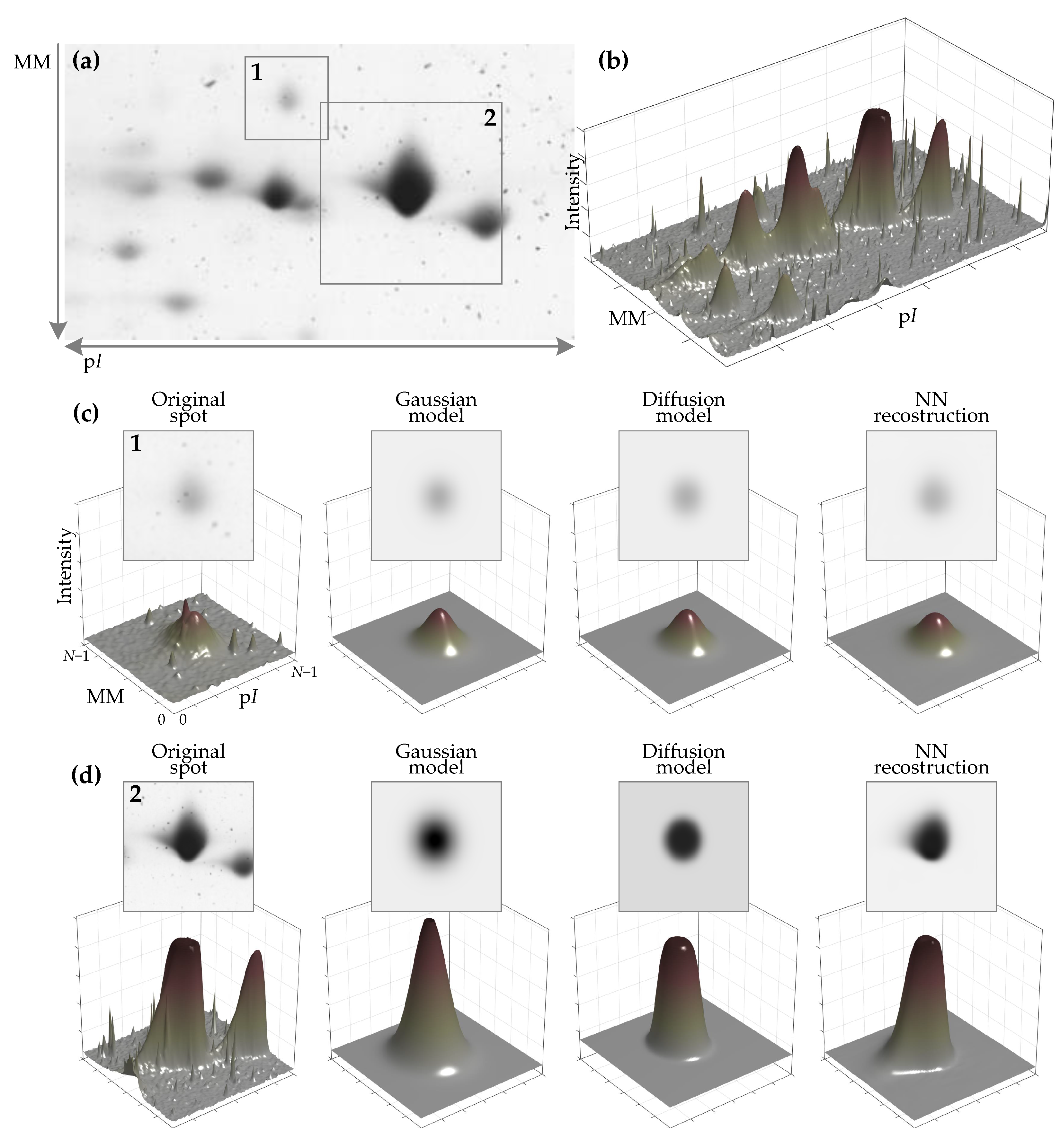
The challenges of 2D electrophoresis gel (2DEG) image analysis. The minimal outcome of the analysis of 2DEG images includes information about visible protein spots: its center coordinates, the intensity of the spot peak, the background intensity, the boundaries of the spot, and the spot’s integrated intensity (volume) are of interest. A small area of a 2DEG image is presented in the usual form (a) and as a 3D surface of its inverted intensity (b). One approach to estimating the spot’s parameters is to model the spot. Modeling of the protein spot additionally allows isolating the spot from noise and separating it from uneven background. The noise is more clearly visible in 3D surface plots (b–d). Modeling results of two spots (areas 1 and 2 of (a)) are shown in (c,d). The results of three modeling methods are: the Gaussian and diffusion process models, commonly met in the literature, are shown in the 2nd and 3rd columns), and the result of spot reconstruction using the method presented in this research based on machine learning tools is shown in the last column. Modeling using Gaussian and diffusion models additionally requires an initial spot mask. The presented method is able to reconstruct the main spot, eliminate the noise, and remove additional spots without any such mask. Additionally, the presented method is better at spot shape and background reconstruction.
Figure 1.
The challenges of 2D electrophoresis gel (2DEG) image analysis. The minimal outcome of the analysis of 2DEG images includes information about visible protein spots: its center coordinates, the intensity of the spot peak, the background intensity, the boundaries of the spot, and the spot’s integrated intensity (volume) are of interest. A small area of a 2DEG image is presented in the usual form (a) and as a 3D surface of its inverted intensity (b). One approach to estimating the spot’s parameters is to model the spot. Modeling of the protein spot additionally allows isolating the spot from noise and separating it from uneven background. The noise is more clearly visible in 3D surface plots (b–d). Modeling results of two spots (areas 1 and 2 of (a)) are shown in (c,d). The results of three modeling methods are: the Gaussian and diffusion process models, commonly met in the literature, are shown in the 2nd and 3rd columns), and the result of spot reconstruction using the method presented in this research based on machine learning tools is shown in the last column. Modeling using Gaussian and diffusion models additionally requires an initial spot mask. The presented method is able to reconstruct the main spot, eliminate the noise, and remove additional spots without any such mask. Additionally, the presented method is better at spot shape and background reconstruction.

Figure 2.
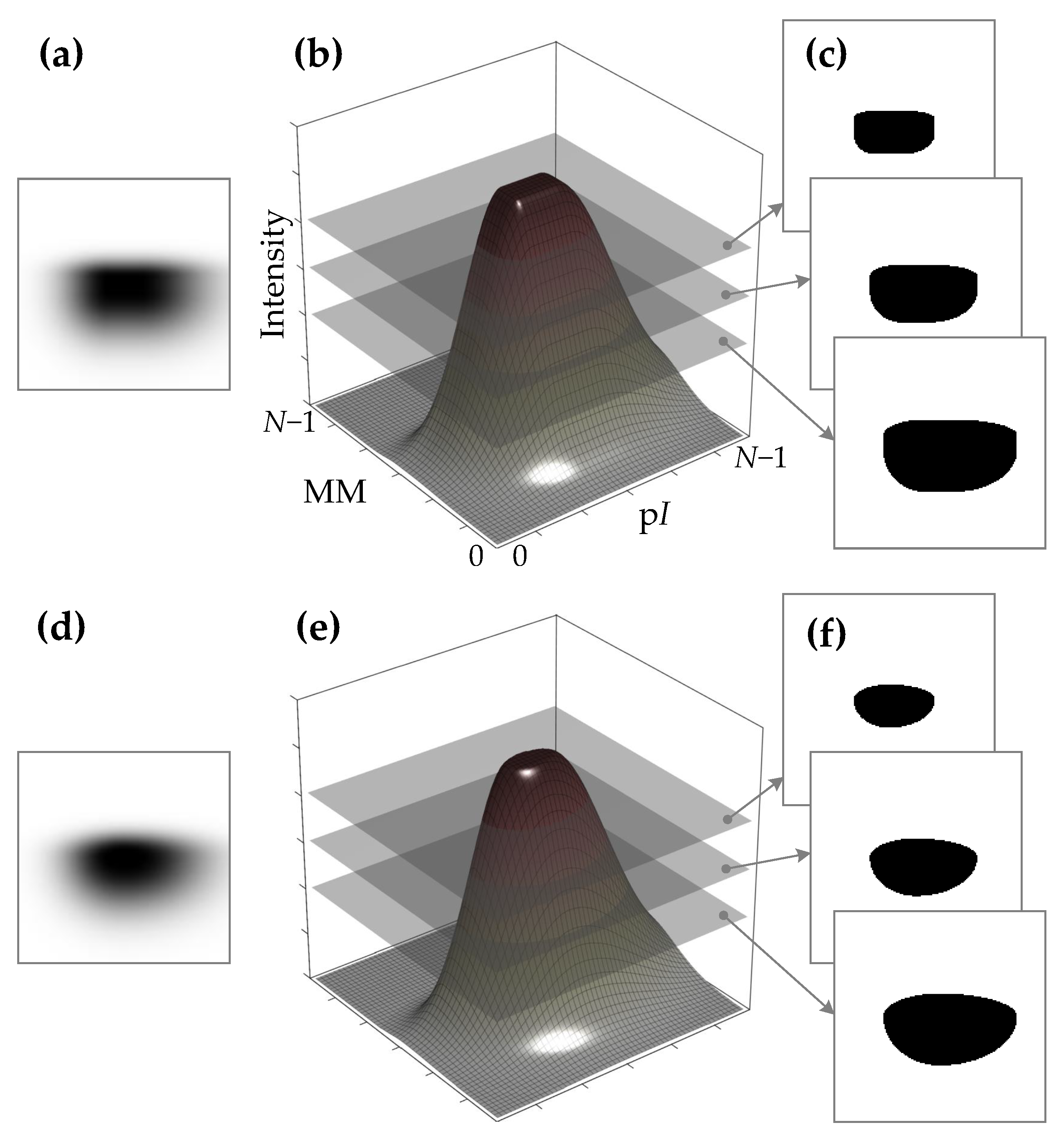
Results of the two approaches to generating the synthetic protein spot: by the outer product of two vectors that correspond to the vertical and horizontal sections of the spot (a–c) and by elliptical interpolation of the vertical and horizontal sections of the spot (d–f) as described in the current research. The approaches reside at different sides of the speed–fidelity scale. A faster construction of the spot leaves some undesirable artifacts in the spot appearance (a–c). In cases when generating more extremely saturated spots (spots with larger plateaus on the top), the horizontal sections of the spots start to lose smoothness (c). When the process of spot shape construction is not constrained by the time limits, a more computationally intensive approach allows for generating smoother saturated spots (d–f).
Figure 2.
Results of the two approaches to generating the synthetic protein spot: by the outer product of two vectors that correspond to the vertical and horizontal sections of the spot (a–c) and by elliptical interpolation of the vertical and horizontal sections of the spot (d–f) as described in the current research. The approaches reside at different sides of the speed–fidelity scale. A faster construction of the spot leaves some undesirable artifacts in the spot appearance (a–c). In cases when generating more extremely saturated spots (spots with larger plateaus on the top), the horizontal sections of the spots start to lose smoothness (c). When the process of spot shape construction is not constrained by the time limits, a more computationally intensive approach allows for generating smoother saturated spots (d–f).

Figure 3.
Overview of the generation process of the synthetic protein spot dataset. Outcomes of the workflow steps (image samples) are presented on the side and linked by the curvy dashed lines. The whole data generation workflow may be divided into two basic stages: offline data generation and online data augmentation. The offline stage is more computationally demanding and is performed before training the neural network (NN)-based protein spot model. The online augmentation step is performed during the training process. The whole workflow provides training samples consisting of image pairs: an image corrupted by various noise input and a clean target image. The target images may be of two types, depending on NN’s defined task: with background (if NN must learn to reconstruct spots with the background retained) or without background (if NN must learn to reconstruct spots without the background).

Figure 4.
Overview of the generation process of the protein spot prototype (primary spot). Outcomes of the workflow steps (image samples) are presented on the side and linked by the dashed lines. The color of line indicates the same 1D protein spot edge template in the plots.
Figure 4.
Overview of the generation process of the protein spot prototype (primary spot). Outcomes of the workflow steps (image samples) are presented on the side and linked by the dashed lines. The color of line indicates the same 1D protein spot edge template in the plots.

Figure 5.
Visualization of the generation of varying background templates. Four samples of backgrounds are presented. Each plot shows a randomly generated grid of points and a fitted polynomial surface of degree 5 in x and y directions.
Figure 5.
Visualization of the generation of varying background templates. Four samples of backgrounds are presented. Each plot shows a randomly generated grid of points and a fitted polynomial surface of degree 5 in x and y directions.

Figure 6.
Visualizations of the functions used to create 1D protein spot edge templates. The graph shows the plots of the functions: Gaussian (a), simplified diffusion process (b), spline (c), Fuzzy Logic generalized membership bell-shaped function (d), sigmoid (e), raised cosine (f). The horizontal axis spans the distance from the spot center to the edge of the image sample (in this research, px, half of the image patch size, which is px). The abilities of the functions to imitate the shapes of protein spots are revealed by random sampling parameters from the defined range and plotted as thin lines. Thick lines represent the cases when parameters are being set to the minimum or maximum of the defined range (refer to Table 1).

Figure 7.
Structure of the protein spot reconstruction algorithm. The autoencoder (AE) is the core part of the algorithm. In addition to the AE, there is a separate branch for the prediction of spot parameters from the bottleneck features (spot parameterizer). In this experiment, the spot parameterizer predicts the peak intensity and integrated intensity of the spot (). Configurations of the encoder, decoder, and parameterizer are presented in blocks framed by the dashed line, showing the number of filters and kernel sizes of the convolutional layers, the number of units in dense layers, and the output shapes of all the layers. The loss of the current model has two components: mean absolute error (MAE) of spot reconstruction and MAE of spot parameter prediction.

Figure 8.
Protein spot reconstruction results: experiments using synthetic (a) and real (b) images of protein spots. Model performance is compared by normalized sum of squared error (NSSE) (lower is better). Models “M2G”–“MSAS” are the baselines, and “AE+B” and “AE−B” are the developed autoencoder-based spot models. Experimental cases: “=1spot”/“>1spot”—one or more spots in the input image; “+Mask”/“−Mask”—spot mask is provided or not (mask is used by the baseline algorithms); “+Noise”/“+Bckg”—input images may be corrupted by Gaussian noise or by slowly varying background. Please refer to the text of Section 3 for more details on the models and for the description of the experimental case notation used in the legend.

Figure 9.
Results of protein spot key parameter estimation: peak intensity (a) and integrated spot intensity (volume) (b). Model performance is compared by normalized mean of squared error (NSSE) (lower is better). Models “M2G”–“MSAS” are the baselines, and “AE+B*r”, “AE−B*r”, “AE+B*p”, and “AE−B*p” are the developed autoencoder-based spot models. Experimental cases: “=1spot”/“>1spot”—one or more spots in the input image; “+Mask”/“−Mask”—spot mask is provided or not (mask is used by the baseline algorithms); “+Noise”/“+Bckg”—input images may be corrupted by Gaussian noise or by slowly varying background. Please refer to the text of Section 3 for more details on the models and for the description of the experimental case notation used in the legend.


Table 1.
Summary of the parameter ranges of the functions used to generate 1D edge templates of protein spots. The generation of 1D template samples is done by randomly selecting a function and its parameters from the provided intervals.
Table 1.
Summary of the parameter ranges of the functions used to generate 1D edge templates of protein spots. The generation of 1D template samples is done by randomly selecting a function and its parameters from the provided intervals.
| Parameter Range | ||||||
|---|---|---|---|---|---|---|
| Function | Parameter #1 | Min | Max | Parameter #2 | Min | Max |
| 1. Gaussian | 2 | 15 | d | 0 | 5 | |
| 2. Diffusion | a | 3.5 | 8 | D | 0.2 | 10 |
| 3. Spline | a | 0 | 5 | b | 5 | 35 |
| 4. FL Bell-shaped | a | 2 | 20 | b | 1.2 | 8 |
| 5. Sigmoid | a | 0.5 | 1 | d | 1 | 20 |
| 6. Cosine | a | 2 | 20 | d | 0 | 10 |
Publisher’s Note: MDPI stays neutral with regard to jurisdictional claims in published maps and institutional affiliations. |
© 2022 by the author. Licensee MDPI, Basel, Switzerland. This article is an open access article distributed under the terms and conditions of the Creative Commons Attribution (CC BY) license (https://creativecommons.org/licenses/by/4.0/).
Share and Cite
MDPI and ACS Style
Matuzevičius, D. Synthetic Data Generation for the Development of 2D Gel Electrophoresis Protein Spot Models. Appl. Sci. 2022, 12, 4393. https://doi.org/10.3390/app12094393
AMA Style
Matuzevičius D. Synthetic Data Generation for the Development of 2D Gel Electrophoresis Protein Spot Models. Applied Sciences. 2022; 12(9):4393. https://doi.org/10.3390/app12094393
Chicago/Turabian StyleMatuzevičius, Dalius. 2022. "Synthetic Data Generation for the Development of 2D Gel Electrophoresis Protein Spot Models" Applied Sciences 12, no. 9: 4393. https://doi.org/10.3390/app12094393
Note that from the first issue of 2016, this journal uses article numbers instead of page numbers. See further details here.