
Research on Improved Deep Convolutional Generative Adversarial Networks for Insufficient Samples of Gas Turbine Rotor System Fault Diagnosis

1
School of Mechanical and Electrical Engineering, Beijing Information Science and Technology University, Beijing 100192, China
2
College of Mechanical Engineering and Applied Electronics Technology, Beijing University of Technology, Beijing 100124, China
3
Key Laboratory of Modern Measurement and Control Technology of Ministry of Education, Beijing Information Science and Technology University, Beijing 100192, China
*
Author to whom correspondence should be addressed.
Appl. Sci. 2022, 12(7), 3606; https://doi.org/10.3390/app12073606
Submission received: 5 March 2022
/
Revised: 27 March 2022
/
Accepted: 29 March 2022
/
Published: 1 April 2022
(This article belongs to the Special Issue Advances in Deep Learning III)
Abstract
:In gas turbine rotor systems, an intelligent data-driven fault diagnosis method is an important means to monitor the health status of the gas turbine, and it is necessary to obtain sufficient fault data to train the intelligent diagnosis model. In the actual operation of a gas turbine, the collected gas turbine fault data are limited, and the small and imbalanced fault samples seriously affect the accuracy of the fault diagnosis method. Focusing on the imbalance of gas turbine fault data, an Improved Deep Convolutional Generative Adversarial Network (Improved DCGAN) suitable for gas turbine signals is proposed here, and a structural optimization of the generator and a gradient penalty improvement in the loss function are introduced to generate effective fault data and improve the classification accuracy. The experimental results of the gas turbine test bench demonstrate that the proposed method can generate effective fault samples as a supplementary set of fault samples to balance the dataset, effectively improve the fault classification and diagnosis performance of gas turbine rotors in the case of small samples, and provide an effective method for gas turbine fault diagnosis.
1. Introduction
As internal combustion type rotating power machinery, gas turbines are the core components of power equipment in industrial fields, and have rapidly developed and been widely used in other fields such as aerospace, industrial power generation, navigation, and land transportation. The reliability and safety of gas turbines are receiving more and more attention. Due to various unavoidable factors, the gas turbine has various failures, and the predetermined function is reduced or even completely lost. As a result, serious or even catastrophic accidents occur, and huge economic losses are felt by enterprises and even industries [1].
Common gas turbine faults are divided into two categories. The first is related to aerodynamics or performance-based faults, such as thermal distortion, compressor erosion and corrosion, compressor fouling, turbine fouling, turbine erosion and corrosion, blade rubbing, etc. Gas Path Analysis (GPA) is an effective technical means for forecasting these faults [2]. At present, data-driven machine learning has been used for gas path diagnosis based on fault sample sets, such as Artificial Neural Network (ANN) [3], Support Vector Machine (SVM) [4], Bayesian network [5], and fuzzy logic [6]. The second type of common gas turbine faults is related to mechanical properties, such as shaft misalignment, rotor dynamic imbalance, bearing defects, and oil film instability [7]. For such faults, there are many technical means, such as oil chip analysis, vibration analysis, acoustic analysis, thermal aging, load analysis, metal temperature, stress analysis, and so on.
Vibration monitoring [8] is one of the commonly used methods for gas turbine condition monitoring and fault diagnosis. Effective condition monitoring, fault diagnosis, and maintenance are effective means to ensure the safe, reliable, and stable operation of gas turbines. Through vibration sensors arranged in the casing and other parts of the gas turbine, the vibration signals of the gas turbine are obtained and analyzed with certain signal processing technology to extract the vibration characteristics for locating the fault and finding out the cause of the fault, thereby providing a basis for the diagnosis, evaluation, and decision making concerning the gas turbine. Vibration condition monitoring can reduce downtime for maintenance, reduce maintenance costs, reduce safety accidents, and ensure the normal operation of equipment to improve its reliability [9].
The rotor system is the most important component in a gas turbine. Due to the complex structure of the gas turbine rotor system and strict assembly process, it plays a vital role in the healthy operation of the gas turbine. The rotor system runs under harsh working environments with high temperatures, high pressure, and high speeds, and it is easy to collide with the internal structure. Once a failure occurs, the rotor will deviate from the normal working state, and it will cause significant damage to the gas turbine in severe cases [10].
In gas turbine rotor systems, rotor imbalance faults, rotor misalignment faults, rotor rub impact faults, rotor thermal bending, and other faults emerge. Through vibration monitoring and by analyzing the vibration signal of the rotor, fault diagnosis and condition evaluation can be carried out to provide suggestions for maintenance personnel that are of great significance to ensure the safe and reliable operation of gas turbine rotor systems.
The development of gas turbine condition monitoring and fault diagnosis methods can be divided into three categories: methods based on qualitative experience knowledge, methods based on model analysis, and data-driven methods. The method based on qualitative empirical knowledge relies on the manual judgment of field experts and entails simple processing of the monitoring data. In the method based on model analysis, sensors are used to monitor each component of the engine, signal processing is performed, and engine mathematical models, statistical analysis models, or artificial intelligence pattern recognition models based on observation data are established. In the data-driven methods, mathematical models, statistical analysis models, and machine learning models are integrated, and expert experiences, knowledge about engines, and information such as engine monitoring data are merged. Among such methods, the intelligent diagnosis method uses many new methods and means, including fuzzy logic, expert system, and artificial neural network [11]. With the continuous application development and improvement of these methods, the condition monitoring of mechanical equipment will gradually be systematic and intelligent. At present, data-driven diagnostic methods mainly include statistical analysis methods, signal processing methods, and artificial intelligence-based methods [12]. Among them, statistical methods are limited to statistical analysis theories, and their scope of application is limited. Signal processing technology is an important means of mechanical vibration fault analysis, represented by Fourier transform [13], wavelet packet analysis [14], Hilbert–Huang transform [15], and other methods. The signal processing method is based on the signal analysis technology to extract the time–frequency domain characteristic parameters and characterize system state, and data loss still occurs in this process [16].
The fault diagnosis method based on artificial intelligence technology does not require the establishment of professional related mathematical models, and the application of advanced classification and regression algorithms to historical data or running logs can realize fault diagnosis [17]. In many fault diagnosis methods based on artificial intelligence technology, typical representatives are methods based on artificial neural networks [18], methods based on support vector machines [19], and methods based on fuzzy logic [20]. At the same time, the classic classification methods of machine learning also include decision trees, random forests, and extreme decision trees. With the breakthrough in the performance of artificial intelligence algorithms, many advanced data processing methods, image recognition tools, and data analysis algorithms have gradually been applied in the prototype design, method optimization, and fault diagnosis of gas turbines [21,22,23,24], and many results have been achieved.
The progress of deep learning also has some applications in gas turbine fault diagnosis [25,26,27]. However, most of the intelligent diagnosis methods based on deep learning require sufficient data samples, and the problem of fault data scarcity in the actual engineering of gas turbines is a big challenge for gas turbine application. At present, due to the complex structure of the large gas turbine rotor system and the limited test conditions, there are only some fault data under each working condition of practical running, and some faults have never occurred. For the fault types not involved in the sample set, it is difficult to obtain accurate diagnosis results by using deep learning methods. In addition, individual differences such as equipment manufacturing and installation errors and changes in operating conditions make the application scenarios of equipment complex and changeable; thus, the applicability of the method needs to be improved.
Therefore, how to solve the problems of a small sample, insufficiently labeled data, and low diagnosis accuracy has become the top priority in fault diagnosis and identification. Generative Adversarial Network (GAN) as an artificial intelligence method provides a good technical means to solve this problem [28,29]. Its unique adversarial idea makes it stand out among many generator models, and it has wide applications in sample generation, data enhancement, and other fields. In the Generative Adversarial Network, the existence of the generator means that the sample size and completeness are no longer the key factors that affect the accuracy of the entire network. Luo et al. [30] proposed a new generative adversarial learning model to deal with the fault diagnosis of rotating machinery. The generator can generate fault data with higher reliability to improve the fault diagnosis dataset. Wang et al. [31] aimed at the problem of sample imbalance, obtained the fault characteristics of the signal through GAN, and generated new fault samples. Viola et al. [32] proposed a generative model based on Generative Adversarial Networks to generate synthetic samples that conform to the original data sample distribution, and extended training samples to solve the overfitting problem of the classification model due to insufficient training samples. Li et al. [33] used the Enhanced Generative Adversarial Network to compare the probability distribution between the generated signals and the real signals, and generated the fault signals for rotating machinery fault diagnosis.
The Deep Convolutional Generative Adversarial Network (DCGAN) is an improvement model of GAN [34]. It mainly improves the network structure of GAN. It combines the automatic feature extraction layer of the sample with the GAN network, which greatly improves the stability of GAN training and the quality of generated data [35,36]. However, the signal generator of the traditional GAN or DCGAN generates the sample signals based on random data. The random noises generated each time during the operation comprise a special code that only a group of generators can understand, and this code determines how the generated results should be represented. The result generated by using random data as the encoding source has little relation with the original signals, making the generator prone to producing meaningless output, resulting in unstable network training and learning, and low quality of the generated signals. Therefore, an improved method based on the original DCGAN to generate sample data is proposed and applied to gas turbine rotor system fault diagnosis. Firstly, the proposed method combines the data generation ability of DCGAN and the feature extraction ability of Convolutional Neural Network (CNN) to construct a new optimized signal generator, which further improves the quality of generative fault samples for fault diagnosis. Secondly, generative samples are combined with original samples to form feasibility samples and supplement the gas turbine rotor fault dataset, and then the fault samples are adopted to build up the fault diagnosis model. Finally, gas turbine test bench experiments are carried out for fault classification and to verify the proposed method. The main contributions can be summarized as follows:
- (1)
- The Improved DCGAN is proposed, and the generator is optimized by adding a one-dimensional Deep Convolutional Neural Network With a Wide First-Layer Kernel (WDCNN) to the deconvolution layer of the generator, to build a generator containing the gas turbine vibration data features and generate samples with higher quality and similarity to original samples.
- (2)
- The loss function of the generator and discriminator are optimized, and a gradient penalty is adopted to solve the problem of gradient disappearance and improve the applicability of the method. The optimized penalty factor can be adjusted according to the actual situation, which improves the adaptability of the method.
- (3)
- The generated effective fault samples are added to the fault dataset, and the proposed method is validated on the gas turbine rotor system fault data to solve the problem of insufficient gas turbine rotor system fault samples and provide new ideas for gas turbine rotor system fault diagnosis.
2. Theoretical Method Introduction
2.1. Deep Convolutional Generative Adversarial Network
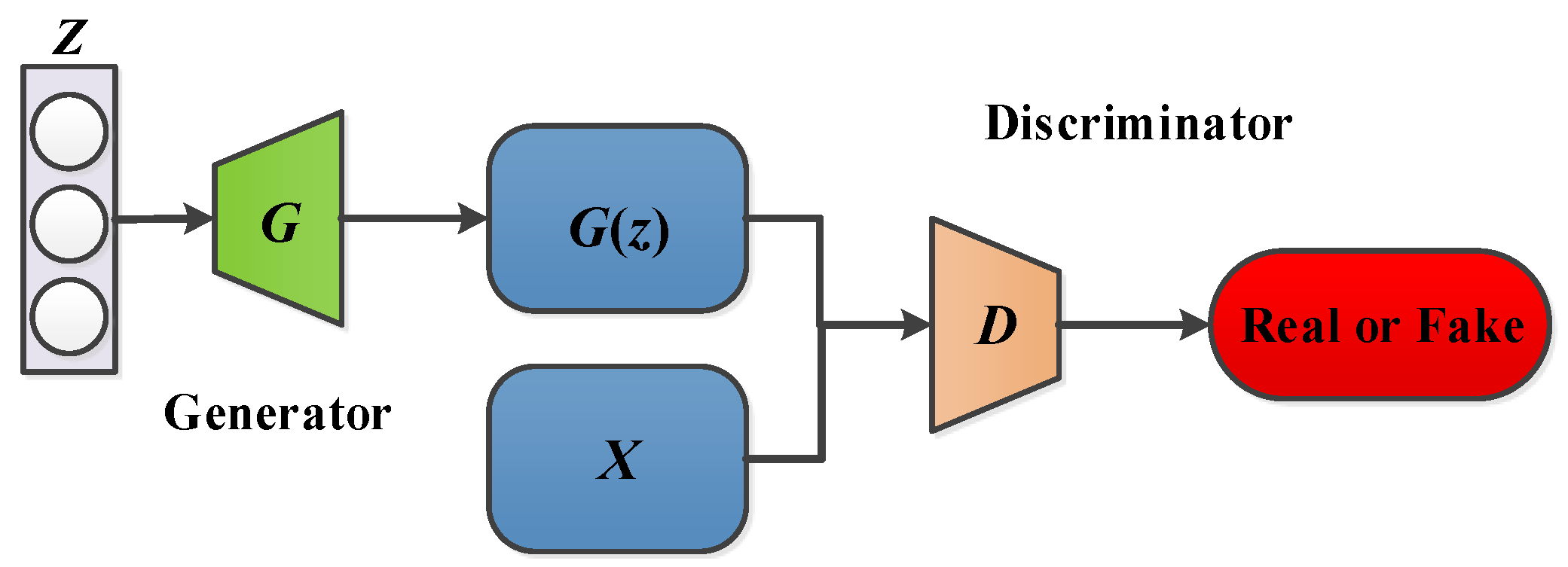
The Generative Adversarial Network is a machine learning architecture proposed by Ian Goodflow in 2014, and it is one of the most promising methods of unsupervised learning in recent years. Due to its outstanding data generative capabilities, Generative Adversarial Networks have been fully applied in many fields, especially in image processing, text generation, audio processing, data enhancement, and sample prediction. The main idea of GAN is derived from game theory, in which a discriminative model and a generative model are set up to compete with each other to improve the learning effect and obtain high-dimensional and complex data distribution of real samples. Its network structure is shown in Figure 1:
The main structure of GAN includes a generator and a discriminator [37,38]. The generator is used to generate real samples, and the discriminator is used to determine real samples and fake samples. The generator inputs a random noise vector (usually uniform or normal distribution) and maps it to a new multi-dimensional data space to achieve a generated fake sample . The discriminator is used to perform classification and to calculate the probability that the testing sample is a real sample. In the training, the generator tries to learn the data distribution of the real sample to generate a fake sample, and the discriminator tries to distinguish the generated fake sample from the real sample. The objective function of the generative adversarial network is as follows:
During the training process of the GAN network, the objective function of is:
The parameters are optimized by Equation (2) to improve . The objective function of is:
Among them, represents the data sample, represents the data distribution of the input noise, represents the sample generated by the input noise, represents the probability that sample determined by the discriminator is the real sample instead of the generated sample. represents the probability of obtaining real data; represents the probability of discriminating real data.
During the training process, alternate iterations are performed. Firstly, the network is fixed, and the discriminator network is trained so that the labels of the training samples are classified correctly with the greatest probability, with maximized and . Then, the network is fixed, and the network is trained to minimize . The training of the generator network puts close to 1, so that the generator loss will be the smallest. The goal of training the discriminator network is to distinguish the real data and the generated data; that is, the discriminator output of the real data is expected to be close to 1, and the output of the generated data is close to 0. Finally, the training reaches a balance, and can estimate the distribution of sample data.
The focus of GAN is to find the Nash equilibrium point, and the goal of the gradient descent method in the neural network is to find the smallest loss function, so in model training, there may be situations where the model cannot converge or the convergence is unstable. Moreover, there may be a pattern collapse phenomenon in GAN; that is, the generated data sample pattern is singular, and it does not cover all categories of real data. Therefore, how to ensure stable training of GAN has always been a difficult topic [33,39].
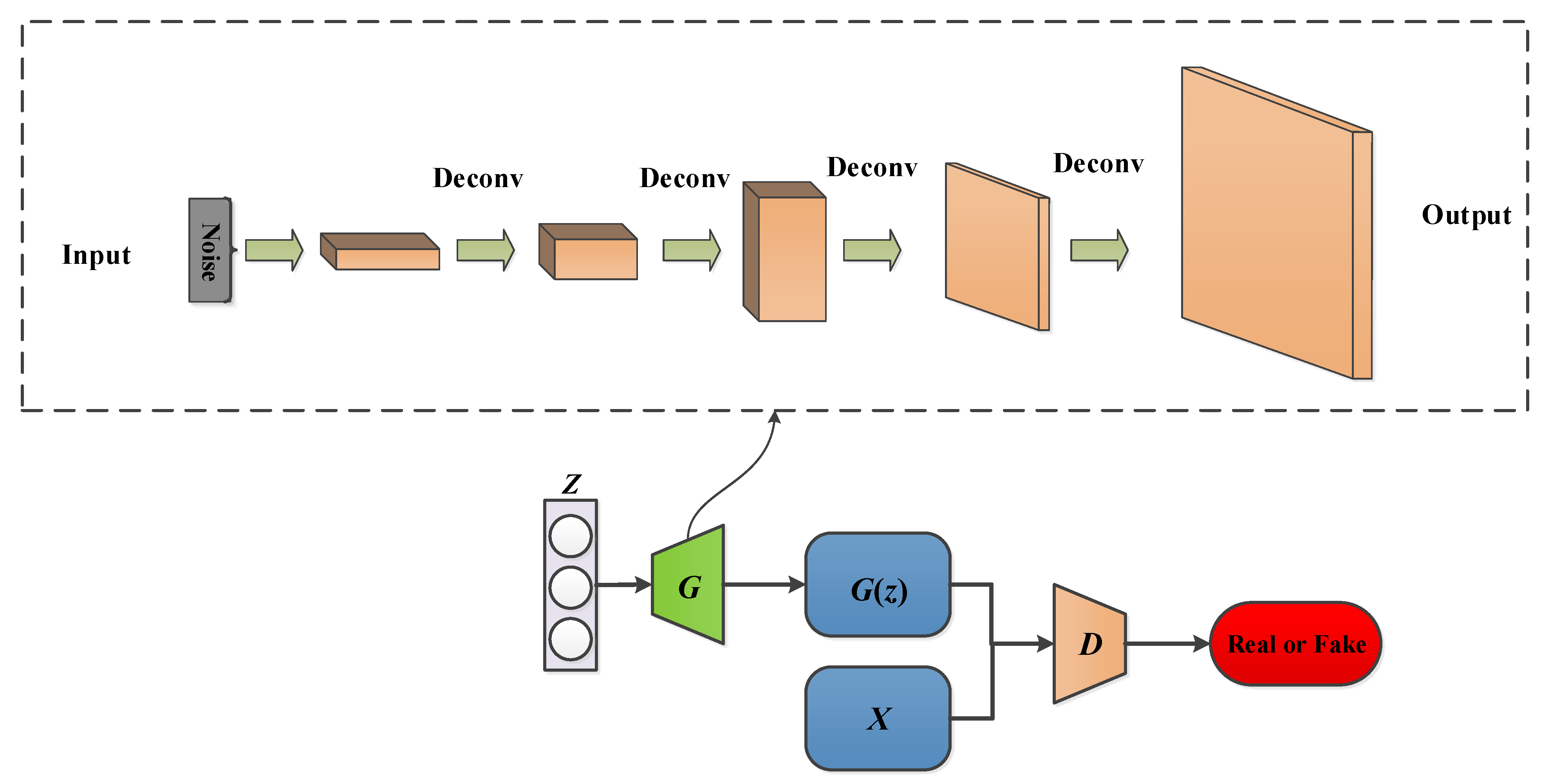
With the continuous intensive research in the field of image and sample generation by the Generative Adversarial Network, many excellent image and sample generation algorithms have emerged. Radford et al. [40] proposed a Deep Convolutional Generative Adversarial Network. By improving the neural network structure in the GAN model, the deconvolution layer innovatively replaced the fully connected layer of the generator in the basic GAN network, thus achieving excellent performance in image generation tasks. As shown in Figure 2, the powerful feature extraction capability of CNN in DCGAN is adopted to improve the learning effect of the generative network. By use of Batch Normalization (BN) in the layer, the generator can learn stably, so that the model can learn better data sample distribution and more stably generate high-quality samples.
DCGAN improves the GAN structure, and greatly improves the stability of GAN training and the quality of generated data [41,42]. Its main improvements are as follows: Convolutional Neural Network is used instead of the original GAN generator and discriminator network structure; in the generator network, micro-step convolution is used instead of pooling layers and fully connected layers; and in the discriminator network, step-size convolution is used instead of pooling layers and fully connected layers. Batch normalization unified operations are added to both the generator network and the discriminator network, and in order to prevent the oscillation and instability of CNN, batch normalization unified operation is not added to the output layer of the generator network or the input layer of the discriminator network. The tanh activation function is used in the output layer of the generator network; the ReLU activation function is used in all rest layers. In the discriminator network, the LeakReLU activation function is used instead of the ReLU activation function to solve the vanishing gradient problem when the discriminator network returns to the generator network. DCGAN greatly improves the stability of GAN training and the quality of the generated results.
2.2. Convolutional Neural Network (CNN)
The Convolutional Neural Network is a typical deep neural network. It reduces the complexity of the network model through the weight sharing method and improves the efficiency of model training. The advantage of this network is that the network model can be trained with input images or signals, eliminating the need for feature extraction. The Convolutional Neural Network consists of an input layer, convolution layer, pooling layer, fully connected layer, and output layer. The input layer realizes the input of the original dataset, the feature is obtained through convolution calculation of the convolution layer, and the pooling layer performs down-sampling operation on the feature image to reduce the data dimension. The number of convolutional layers and down-sampling layers is often determined according to actual conditions. The fully connected layer, just as the neural network, mainly implements data mapping [43,44].
The idea of the convolutional layer is to use convolution kernels to extract local features, which is similar to an automatic feature extraction, which has been widely used in feature extraction, fault diagnosis, and so on. For time series vibration signals, the one dimension Deep Convolutional Neural Network with a Wide First-Layer Kernel (WDCNN) has strong processing capabilities, which can eliminate complex feature extraction and directly perform operations on the sequence. Its main feature is that it has the first layer of a large convolution core and a multi-layer small convolution kernel with the size 3 × 1. It can provide a faster processing speed and it is suitable for real-time fault diagnosis. In the proposed method, the one-dimensional Deep Convolutional Neural Network with a Wide First-Layer Kernel is used for vibration signals’ feature extraction, and it is used as the coding part of the new generator.
The detailed settings of the proposed network structure are shown in Table 1. Vibration signals are used in the input layer. Different kernel sizes, numbers, and strides have been selected to perform the one-dimension convolution operation with an appropriate number. For Conv 1, the kernel size, number, and stride are 32, 20, and 8, respectively. The BN and ReLU activation function are adopted after the Conv layer, and the pooling layers are used to perform the pooling operation. The dropout operation is used after FC1 and FC2, and four different classifications can be recognized.
2.3. Maximum Mean Discrepancy (MMD)
The MMD algorithm is a loss function widely used in transfer learning. It is mainly used to measure the distance of the distribution of two different but related sample data and observe the distribution differences in the two types of sample data [45]. In the proposed DCGAN method, MMD is used to measure the similarity between generated samples and original samples. The smaller the MMD, the better the similarity between the generated sample and the original sample, and the higher the quality of the generated samples. MMD mainly uses high-dimensional mapping functions to find the expected difference in RHKS of the two samples to determine the similarity [46]. Assume the samples obey the distribution and the samples obey the distribution , function maps samples to high-dimensional RKHS, where is the feature space of the sample. The distribution of different samples in RKHS is effectively matched by means of kernel mean embedding. The unbiased estimation of the kernel average embedding is obtained by calculating the expected value and of the sample mapped to the RKHS. is the representation of sample mapped to RKHS through high-dimensional functions. MMD is expressed as follows:
RKHS is a complete high-dimensional inner product space. Dot product operations of and can be calculated with kernel function. Generally, the Radial Basic Function (RBF) is chosen to represent the infinite dimensions Gaussian kernel:
where represents the bandwidth of the Gaussian kernel. We rewrite Equation (5) by Equation (4):
It can be seen from Equation (6) that when and when , it needs to find the mapping function to minimize the , so that the probability distributions of the two samples in RKHS are more similar under the representation to reduce the distribution difference in RKHS. In the Improved DCGAN method, new fault samples are generated by the Generative Adversarial Network, and MMD is used to measure the similarity between generated samples and real samples. The smaller the MMD, the better the similarity between the generated sample and the original sample.
3. Gas Turbine Rotor System Fault Diagnosis Method Based on Improved DCGAN
3.1. The Improved DCGAN
In traditional GAN, random noises are generally used as signal sources to enter into the generator , and new signals and samples are generated after processing by the network. In order to make the generated signal consistent with the real signal, a discriminator is trained and used to identify whether the signal is real data or fake data generated by the generator. The random noise generated each time during the operation is a special code that only a group of generators can understand, and it determines how the generated result should be represented. The result generated by using random data as input barely has a relationship with the original signals, leading to low similarity between the signals generated by the generator and original sample signals and long training time of the network.
Each convolutional layer in a Convolutional Neural Network consists of several convolutional units, and the parameters of each convolutional unit are optimized through the back-propagation algorithm. The purpose of the convolution operation is to extract different features of the input. The first convolution layer may only extract some low-level features such as edges, lines, and corners. The network with more layers can iteratively extract more complex features from the low-level features. The transposed convolutional layer can synthesize pictures or signals based on features, and has been used to generate adversarial networks such as DCGAN.
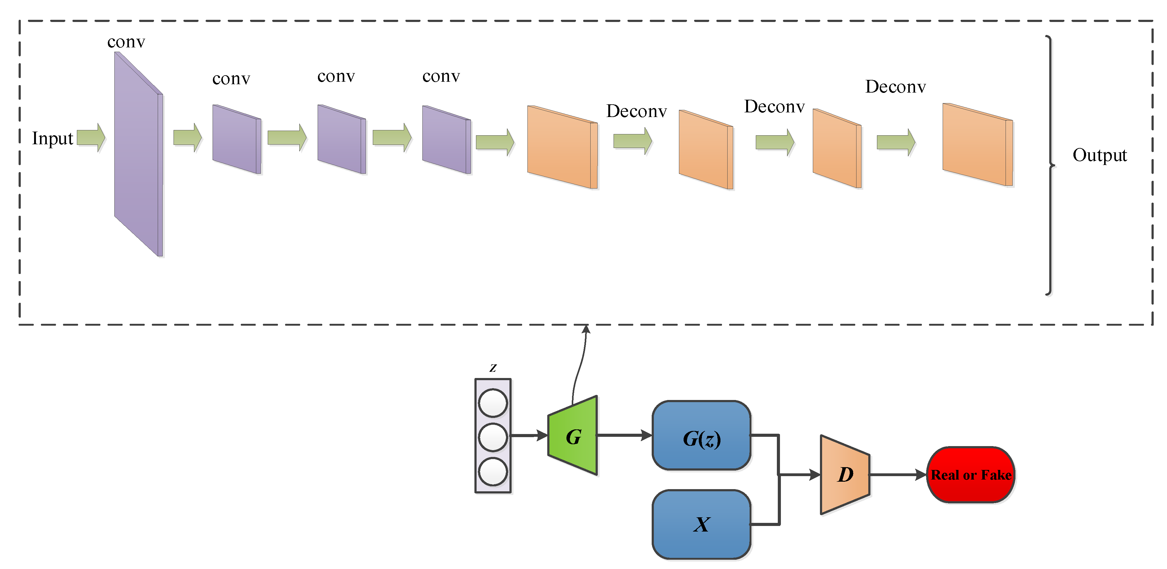
If the advantages of the convolutional layer and the transposed convolutional layer in CNN can be combined, a new generator can be formed. Therefore, in order to obtain the generated samples with higher similarity to the original samples, an Improved DCGAN method is proposed. Figure 3 is shown as the structure of Improved DCGAN. On the basis of DCGAN, the trained WDCNN network is introduced to the generator. The features of input fault signals are obtained through WDCNN network training, so the input contains fault features and the generated samples similar to the original samples are easier to obtain through the generator.
The generator of the Improved DCGAN network consists of three parts: an encoder network, the reshape network, and a decoder network. The encoder network extracts the feature representation of the input signals, and WDCNNs are used as convolutional layers to construct the encoder. The reshape network consists of the project and reshape layer, which upscales the input using a fully connected operation and reshapes the output to the specified size. The decoder network consists of transposed convolutional layers, and takes the transformed features and outputs the final generated signals as samples.
The discriminator examines patches of the input samples and determines the probability of the samples being real or fake. As can be observed, the discriminator has an input layer of 32 × 1. Three hidden layers are employed with LeakReLU as the activation function. Finally, the output layer has a dimension of 256 × 1, which is fully connected with a sigmoid activation function for the real and fake data classification. The kernel size for the CNN is 3 × 1 in all its layers with stride of 2 for all the hidden layers except by the output with stride of 1. The structure parameters and hyper-parameters of Improved DCGAN are shown in Table 2.
3.2. Loss Function Optimization Based on Gradient Penalty
In the process of Generative Adversarial Network training, the loss function is the key to the quality of network learning. If the loss function is incorrect, it will lead to training instability and even exploding gradient problems, and difficulty to train the correct model. The loss function in GAN is used still in DCGAN continuously. Based on DCGAN, an improved method with a gradient penalty is adopted in the proposed method, in which the original loss function in GAN is abandoned and an additional gradient penalty is added to the loss function of the discriminator to solve the vanishing gradient problem and the exploding gradient problem in training. The sparse gradient penalty algorithm is used as the loss function in the process of model training, the negative gradient direction is used as the search direction, and the minimum value is solved along the gradient descent direction, so as to approach the minimum deviation in a recursive way. In the training process, after each forward propagation, the real values of loss value and output value will be obtained. The smaller the loss value, the better the model.
Firstly, the samples and are obtained in the real sample space and the generated sample space , respectively, and then is obtained by random interpolation between the real sample and the generated sample , as shown in Equations (7) and (8):
where represents the random sampling of the samples. According to the joint space sampling , the discriminator output is made, and then the joint derivation is carried out.
where represents the number of batch size samples. Equation (9) is used for the square difference processing to the joint derivative . In order to adapt to the sample characteristics, the joint space sample loss function is finally obtained after the square difference. The gradient penalty term is shown in Equation (10):
where represents the gradient of the discriminator output value in the X direction; represents the mathematical expectation when the input of the discriminator is a random interpolation.
where represents the row number of the matrix ; represents the gradient penalty parameter.
xr ~ Pr, xg ~ Pg, ε ~ U[0, 1]
The original loss function of the discriminator is shown in Equation (12):
where represents the mathematical expectation when the inputs of discriminator are generated samples; represents the mathematical expectation when the inputs of the discriminator are real samples.
In the discrimination of samples, the goal of the discriminator loss function is to reduce the gap between the predicted value of the model and the real value as much as possible. The differences between the loss functions of the discriminator discriminating real and fake samples are weighted and the final discriminator loss function is obtained.
In the loss function of the generator, since the problem solved by the generator is different from that of the discriminator, the loss in the model is mainly caused by convolution processing. The loss caused by joint sampling samples is calculated according to the gradient descent method, and the loss function formula is as follows:
The final generator loss function is as follows:
where represents the gradient penalty parameter of the generator, which can be used to adjust the intensity of gradient penalty.
Compared with DCGAN, the new gradient penalty term will make the overall training of the Deep Convolution Generative Adversarial Network with a gradient penalty more stable, and the convergence and training speed faster.
3.3. The Proposed Gas Turbine Rotor System Fault Diagnosis Method
In traditional Generative Adversarial Networks, random data are used as the encoding source to generate samples. In order to improve network training stability and the generated signals’ quality, the inputs introduce fault features in relation to the original signals. According to the Improved DCGAN structure and optimized loss function, an improved method is proposed, which can be applied to gas turbine rotor fault diagnosis under different unknown conditions with small labeled samples, with the purpose of generating effective sample data and supplying a dataset for fault diagnosis. Figure 4 is a flow chart of the proposed gas turbine rotor fault diagnosis method. The whole process is summarized as follows:
Firstly, accelerometers installed on different parts of the gas turbine are adopted to collect vibration data, and then the obtained signals are preprocessed by time domain and frequency domain analysis. Combining the analysis with expert diagnosis, labeled samples are obtained and the data are divided into the training set and testing set.
Secondly, the fault samples are adopted as the input of the proposed DCGAN network to generate fault samples. The one-dimensional CNN network suitable for vibration signal feature extraction is constructed, and the network and parameters are used for the generator of the Improved DCGAN network, and a new generator for feature extraction of the actual sample data is formed to continually generate new associated samples.
Thirdly, the sample maximum mean difference (MMD) method is used to determine the mean difference between the generated signal and the real signal, and combine the generated data that meet the requirements with the original small sample data to form a new dataset.
Lastly, fault classification and diagnosis are performed on the generated new sample set, and comparisons of results and accuracy analyses are performed to verify the method.
4. Gas Turbine Test Bench Experiment and Fault Diagnosis
4.1. Experiment and Data Acquisition
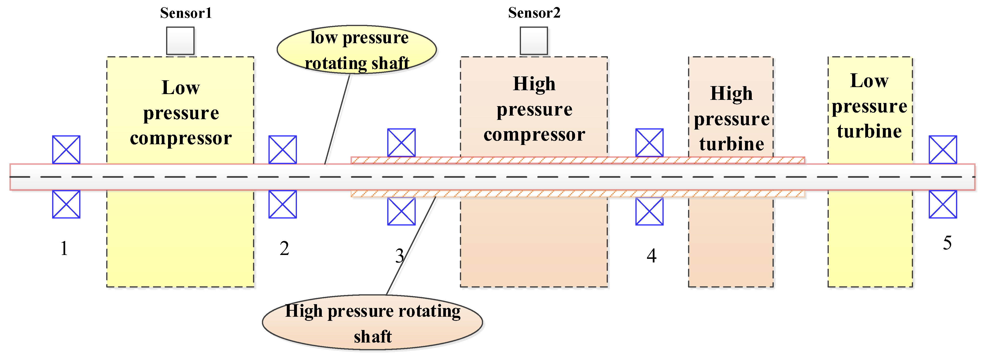
To further verify the performance of the proposed method, the gas turbine rotor system fault experiment from the test bench is adopted. The rotor system of a gas turbine is shown in Figure 5, which is mainly composed of a compressor, turbine, rotating shaft, and so on. The low-pressure turbine is connected to the low-pressure compressor through the low-pressure rotating shaft, and the high-pressure turbine is connected to the high-pressure compressor through the high-pressure rotating shaft sleeved on the low-pressure rotating shaft. Due to the complex and high-temperature internal environment of gas turbines, the whole machine vibration measurement is often used in the engineering application. Through multiple experiments and analyses at different positions and angles, as shown in Figure 5, a speed sensor (sensor 1) is installed on the radial position at the front end of the low-pressure compressor casing as the front measuring point, a speed sensor (sensor 2) is installed at the radial position of the casing between the high-pressure compressor and the combustion chamber as the back measuring point, and the rotor speed sensor for measuring high- and low-pressure rotor speed is installed inside the gas engine. The numbers 1–5 in the Figure 5 are the support points for high- and low-pressure rotor, among which, 1, 2 and 5 are the low-pressure rotor support points, and 3 and 4 are the high-pressure rotor support points.
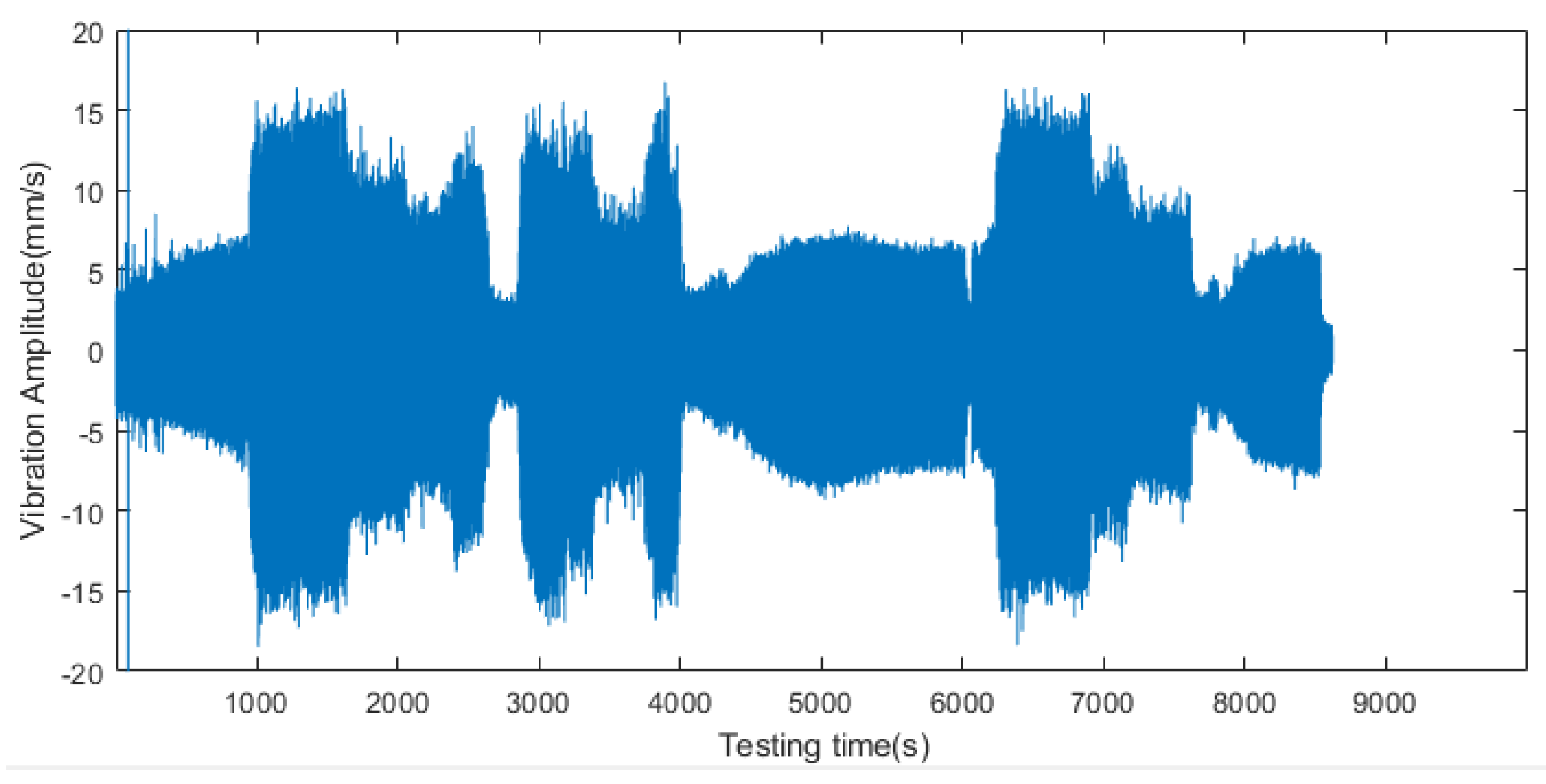
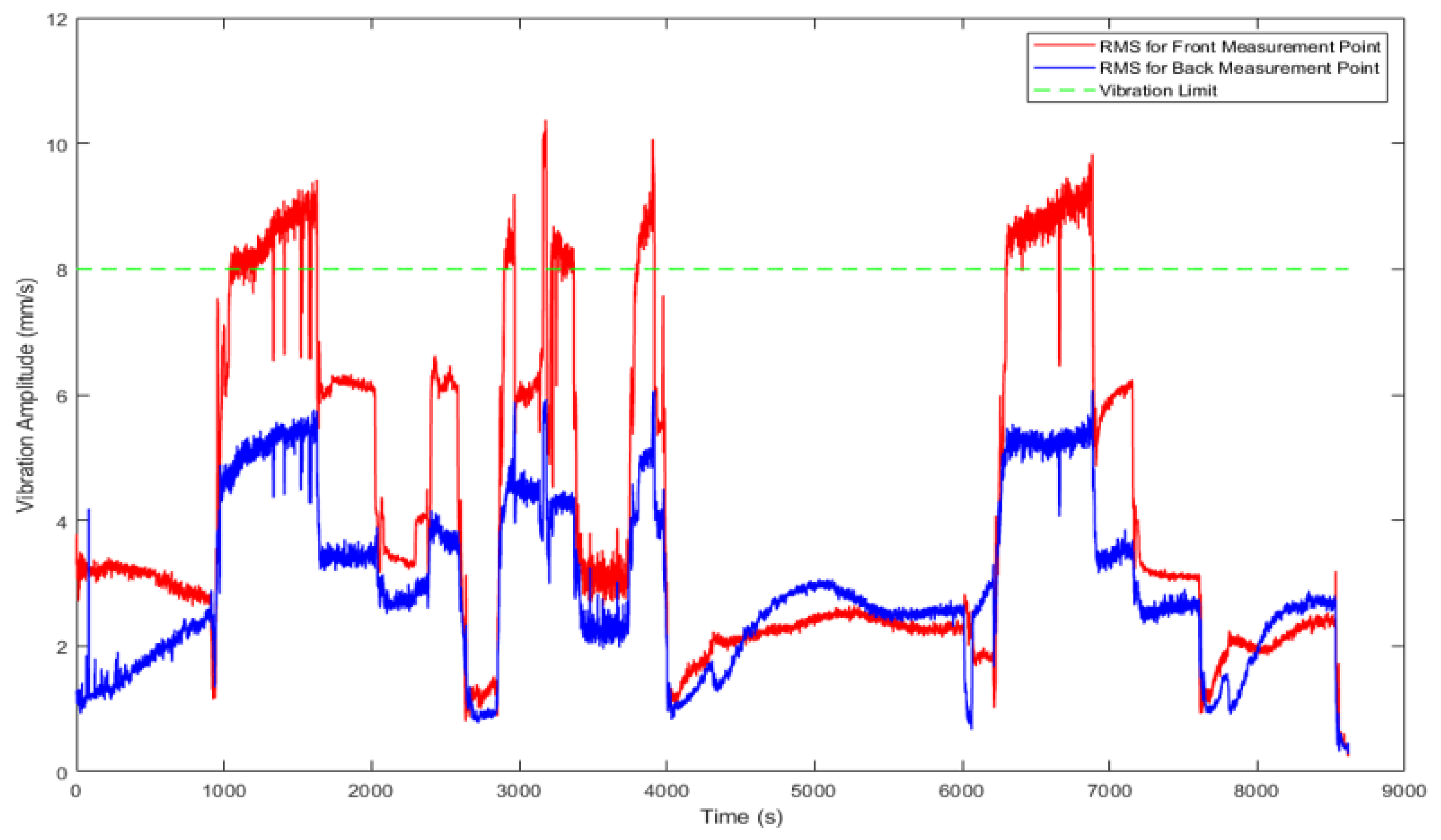
The sampling frequency is 6000 Hz, and the experiment time lasts 8000 s. In the actual operation of the gas turbine rotor system, the time domain statistics in the vibration signals will change with the change in the working conditions and state of the gas turbine rotor system. Therefore, the time domain analysis of gas turbine rotor system vibration signals can be used to preliminarily observe and judge the state and trend of the rotor system, and further for the gas turbine rotor system fault diagnosis and analysis. The vibration signals collected by the gas turbine sensor are shown in Figure 6, and the effective values of gas turbine vibration signals in the time domain can be obtained. From Figure 6, it can be seen that the amplitude of the front measuring point vibration data is large and exceeds the limit in some time periods, and by analysis, it can be concluded that faults may occur. For further analysis, the root mean square (RMS) values of vibration signals are calculated and shown in Figure 7.
In Figure 7, the high-pressure rotor speed changes continuously under multiple working conditions; the dotted line is the change in the high-pressure rotor frequency, the green line is the vibration limit value, the red line is the RMS for the front measuring point, and the blue line is the RMS for the back measuring point. It can be found from the gas turbine sensor data analysis that the speed was constantly changing in various working conditions during the experiment. The effective value of the front measuring point vibration signals and the effective value of the back measuring point vibration signals change with the working conditions. Among them, the effective value of the front measuring point vibration signals has the phenomenon of vibrations exceeding the limit for several time periods, and the effective value of the back measuring point vibration signals has never exceeded the limit. It can be found that in multiple periods of time, due to the structure and assembly of the gas turbine, the gas turbine stalls due to the rotation of the high-pressure compressor during the speed-up condition, resulting in air flow excitation, further causing temporary unbalance of the high-pressure rotor, resulting in vibration overrun.
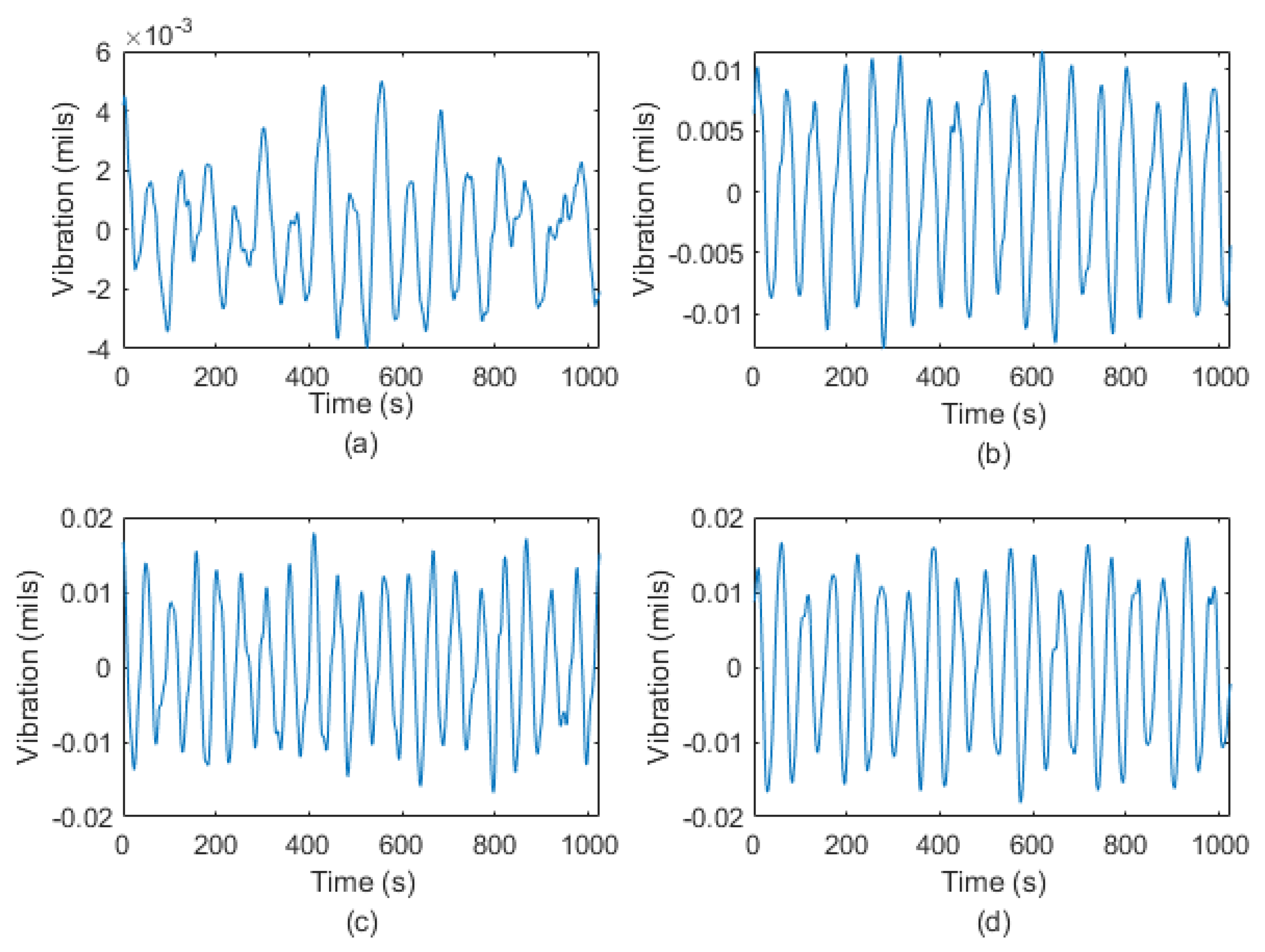
Through further analysis, the pre-measurement vibration data obtained from the gas turbine test bench experiment can be divided into four classes, normal state, air flow excitation, unbalanced, and misalignment, and these test data will be used as the dataset for fault diagnosis. The vibration signals of different faults for gas turbines rotor system are shown in Figure 8.
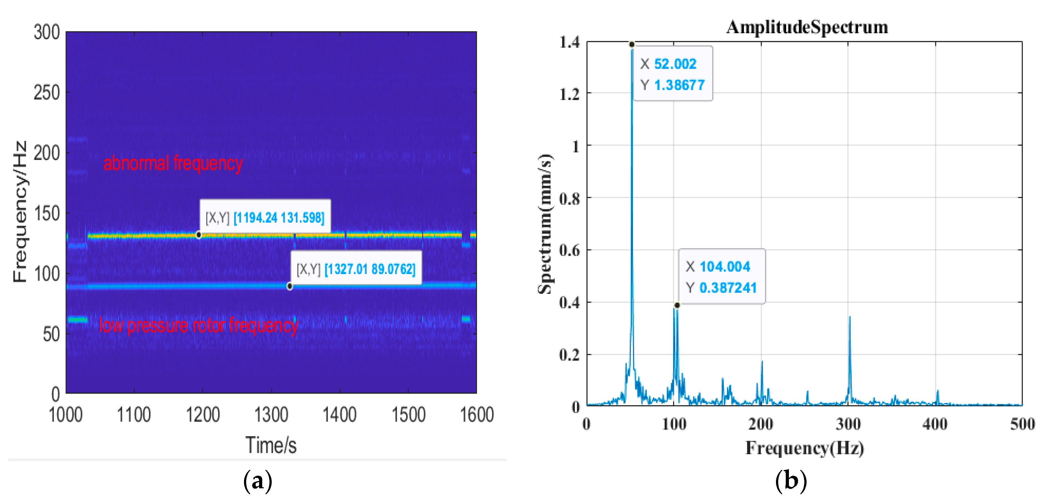
The time–frequency analyses of gas turbine rotor system vibration signals under misalignment and unbalanced states are shown in Figure 9. It can be seen from Figure 9a that the abnormal frequency (131.5 Hz) is about 1.47 times the low-voltage rotating frequency (89.1 Hz), and the frequency is not fixed. After preliminary judgment, it is determined as faults by rotor misalignment. In addition to the abnormal frequency associated with excessive vibration, the double frequency component 101 Hz of low-pressure rotor frequency 52 Hz appears when the high speed drops to slow speed, as shown in Figure 9b. By analysis, this may be caused by the rotor unbalanced. After discussion and consultation with experts, it was preliminarily determined that the abnormal frequency and the reasons for vibration exceeded the standard. Through examining actual faults and machine maintenance, the fault type was determined, and the label was given as the experimental sample.
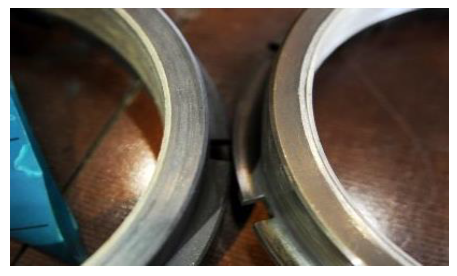
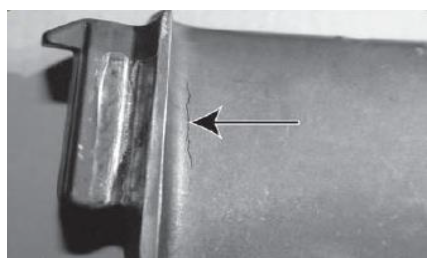
The rotor misalignment could cause the radial double frequency vibration, and axial vibration of the rotor could cause the fatigue damage of the shaft, as shown in Figure 10. If the rotor misalignment lasts for a long time, it will aggravate and cause other more serious faults; thus, it must be effectively identified. The gas turbine rotor system unbalance will directly lead to excessive vibration of the whole machine, which will cause a series of deformed or even damaged elements. The deformation caused by vibrations will produce rub impact, leading to fatigue damage of the rotor or other parts, such as the fatigue crack shown in Figure 11.
4.2. The Training of Improved DCGAN
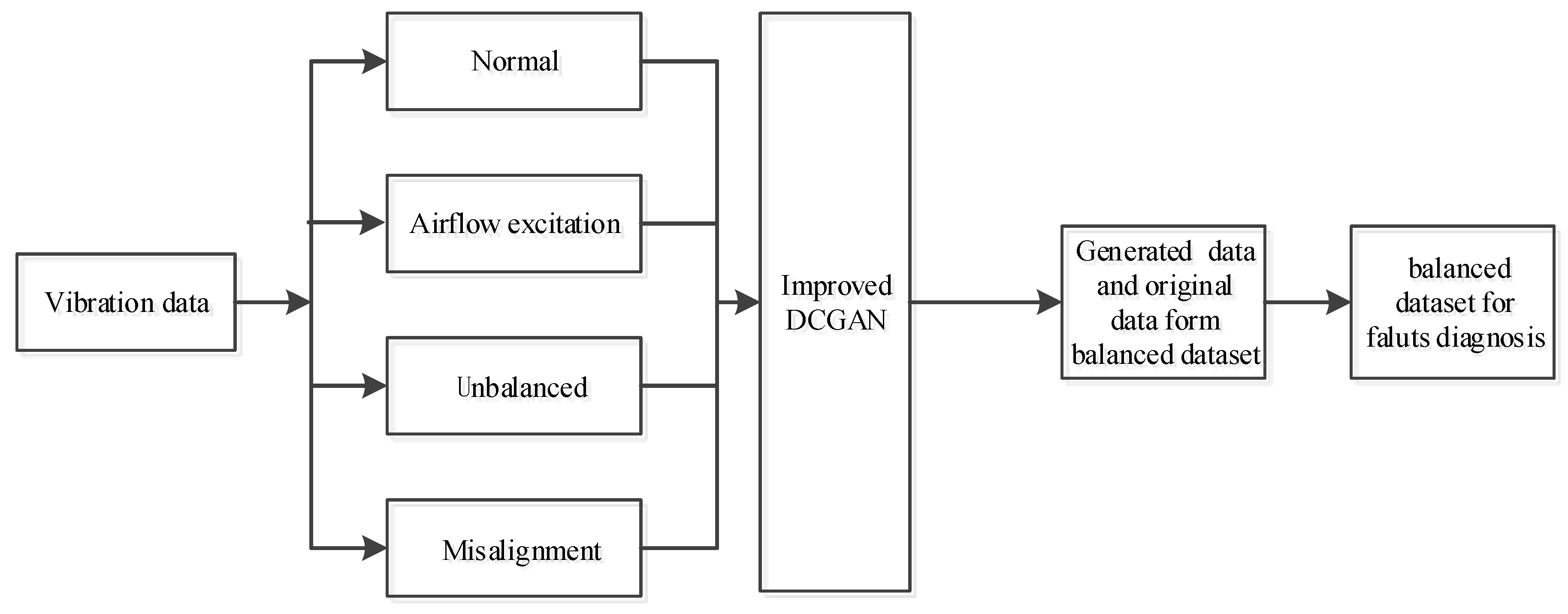
Because the labeling of fault samples requires a lot of experimental and expert experience, the fault samples are not enough. Therefore, in order to improve the accuracy of fault diagnosis, the proposed method is used to generate fault samples with very high similarity with the original samples to supplement all kinds of samples and make up for the imbalance of samples. Figure 12 is the flow chart of gas turbine fault data generation and fault diagnosis of gas turbine rotor systems. The original gas turbine sample is labeled and used as the training dataset; the length of each fault sample is 1024. Then, the labeled samples are taken as the input to Improved DCGAN to achieve the generated samples. The number of samples in the training dataset including generated samples is 1000 for each class. The number of samples in the original training dataset, the training dataset including the generated samples, and the testing dataset are shown in Table 3.
The training parameters of the proposed Improved DCGAN network model are set as follows: the batch size is set as 11, the learning rate is 0.000001, the number of model training iterations is 80,000, the generator gradient penalty parameter is 0.000001, and the discriminator gradient penalty parameter is 10. The optimization method of the generator and discriminator is the Adam optimization algorithm. In order to ensure that the generated signals and the real signals have a large degree of similarity and a small error, the MMD should be set as less than 0.125.
In the adversarial training between the generator and discriminator, the generator tries to generate samples that could cheat the discriminator, and the discriminator learns to distinguish between the generated samples and the real signals with training.
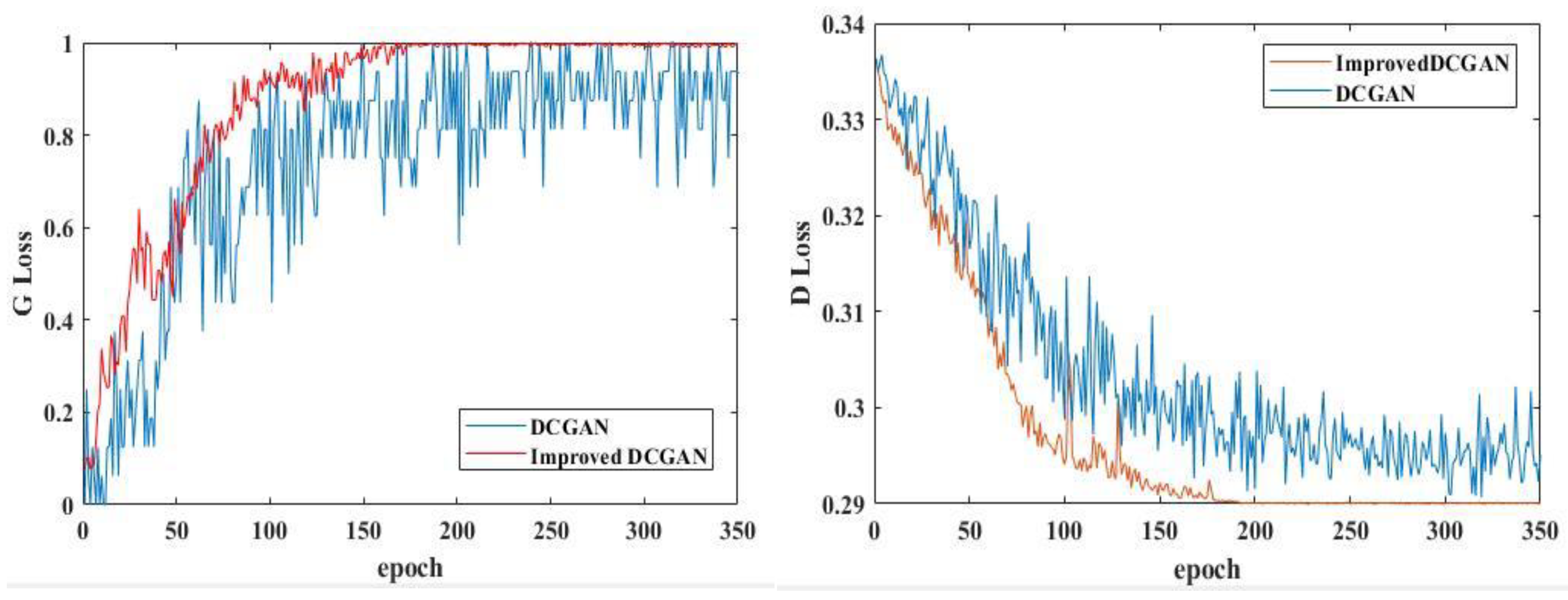
Figure 13 shows the loss function waveform of the generator and discriminator. In adversarial learning between the generator and discriminator, the generated samples increase with iteration, and the loss function gradually changes. At the beginning, the loss of generator is smooth, and then gradually increases and finally tends to be stable. The loss of the discriminator gradually decreases with the training time, and tends to be stable. After adversarial training, the generator generates higher-quality vibration signals.
It can be seen from Figure 13 that compared with DCGAN, the newly added gradient penalty term in the proposed DCGAN made the overall training of the Deep Convolutional Generative Adversarial Network more stable, and the convergence speed faster.
4.3. The Generated Data and Results Comparison
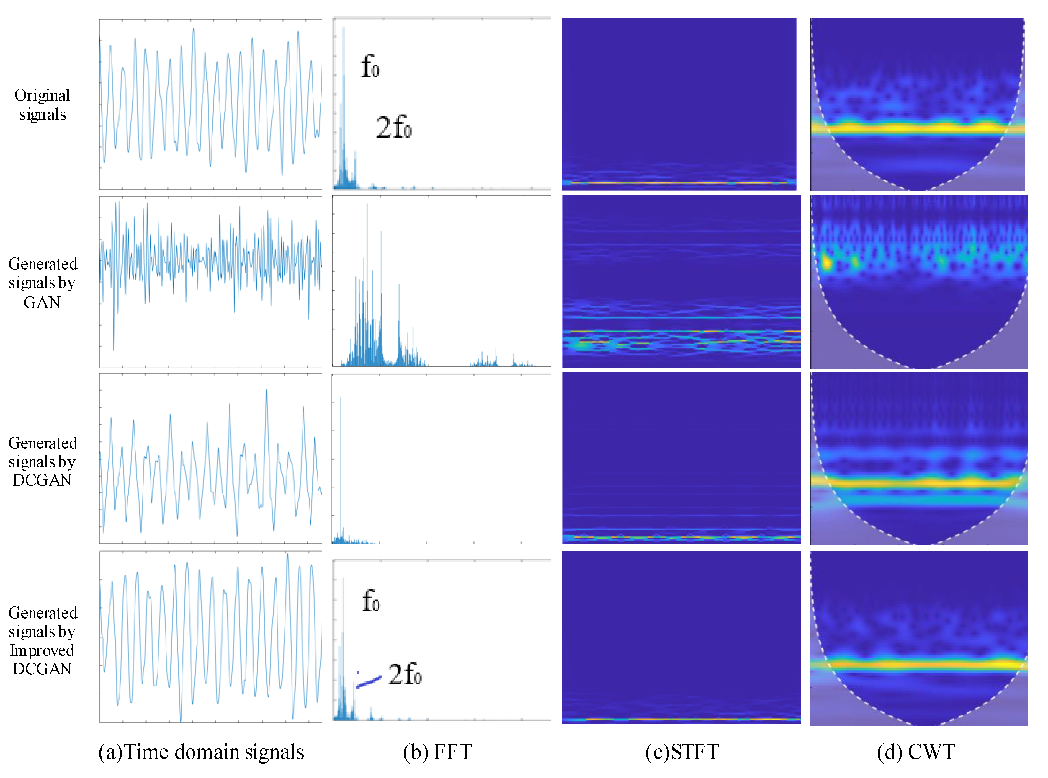
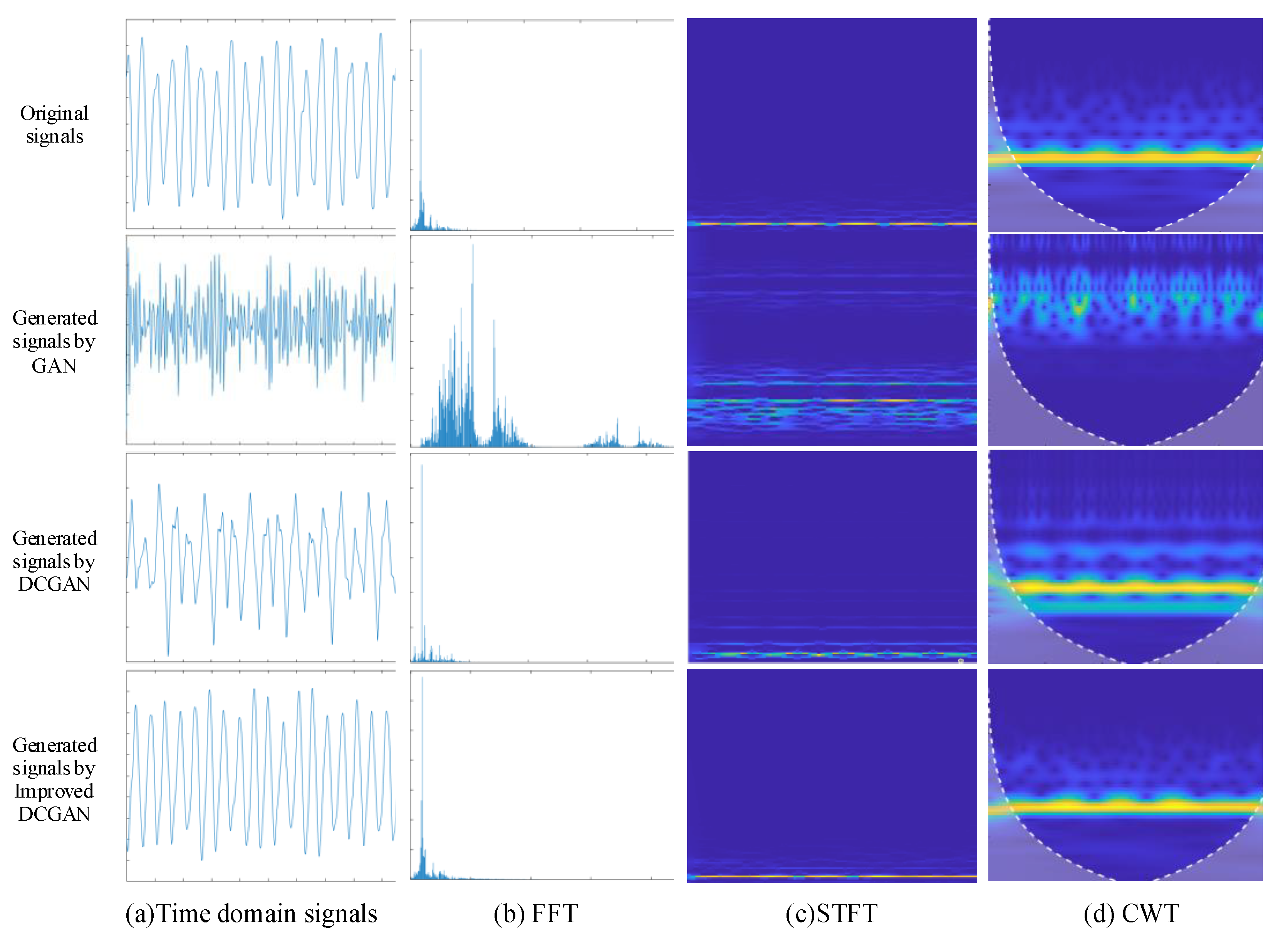
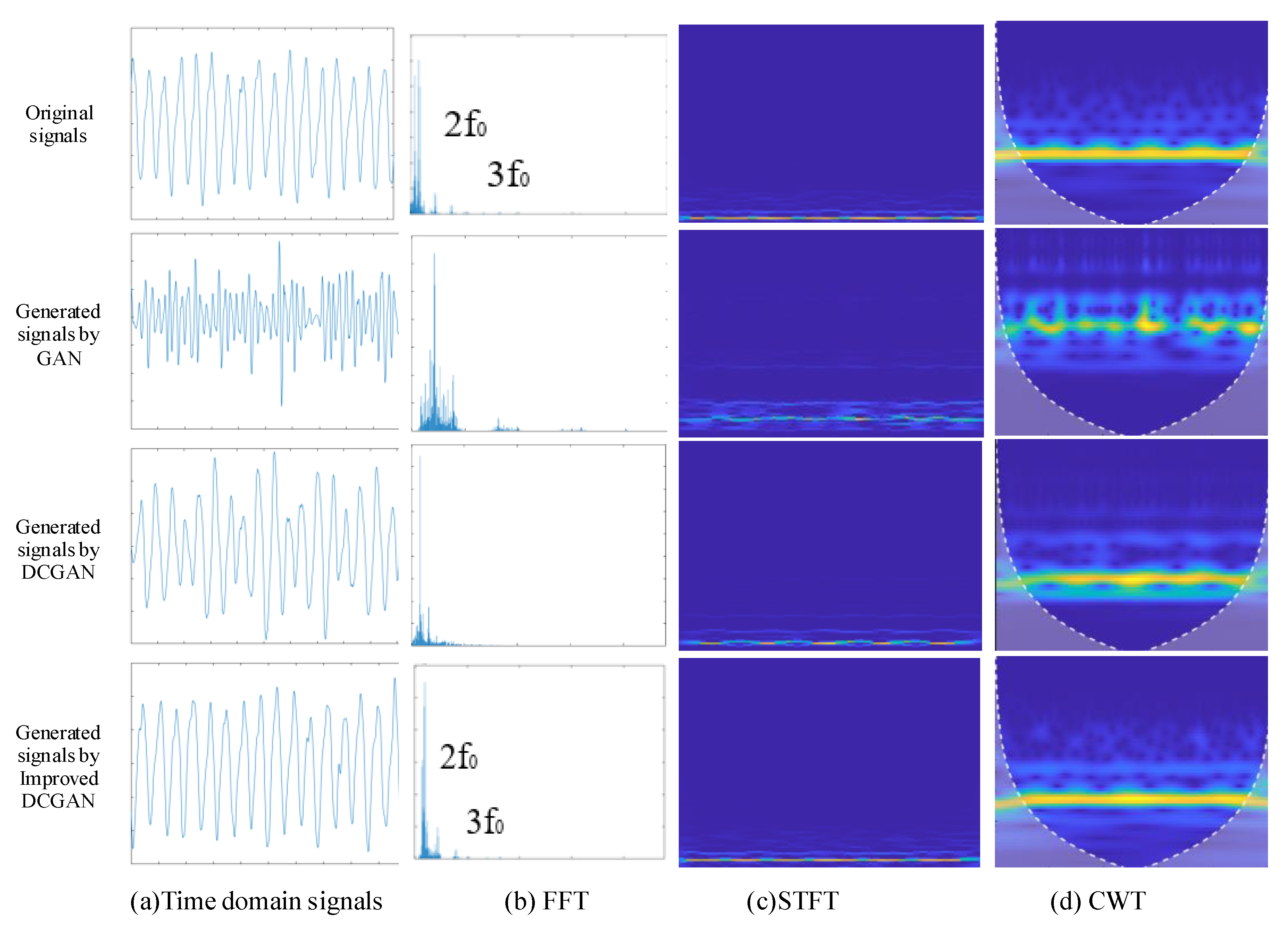
The original signals and generated fault sample signals under four states by the proposed method are demonstrated. Figure 14 shows the generated sample signals of the gas turbine rotor system under the normal state. Figure 15 and Figure 16 show the generated sample signals of the gas turbine rotor system under the airflow excitation state and the unbalanced state. Figure 17 shows the generated sample signals of the gas turbine rotor system under the misalignment state. For comparison, the generated fault sample signals by GAN and DCGAN are also displayed.
Meanwhile, the original signals and generated signals based on GAN, DCGAN, and the Improved DCGAN method are analyzed by frequency domain and time–frequency domain spectrum analysis. In order to better verify the similarity between the generated samples and the original samples, spectrum analysis and Structural Similarity (SSIM) analysis are used for verification.
- (1)
- Spectrum analysis
The similarities between the generated samples and the original samples are analyzed by time domain analysis, Fast Fourier Transform (FFT) spectrum analysis, Short-Time Fourier Transform (STFT) spectrum analysis, and Continue Wave Transform (CWT) analysis. It can be seen from the comparison of spectrum signals in normal states in Figure 14 that the spectrum of the newly generated sample signals is consistent with the spectrum of real sample signals. It can be clearly seen from the FFT and CWT diagrams that the samples generated by the proposed method have the highest similarity with the original signals. The generated samples by GAN and DCGAN are similar to the original samples, but not completely equivalent, and there are small deviations at some peaks.
Figure 15 shows the vibration signals and generated sample signals under airflow excitation from time domain signals, frequency domain, and time–frequency spectrum. It can be seen from the FFT spectrum diagram of the original signals that there are multiple doubling frequency components in the frequency domain, including fundamental frequency f0, double frequency 2f0, and triple frequency 3f0. Meanwhile, it can be seen from the FFT spectrum diagram of generated samples by the proposed method that these frequency features are similar to the features of original signals under air flow excitation, which proves that the key features of the samples generated by the proposed method are consistent with those of original samples, and the quality of the generated samples is high. The samples generated by GAN have no obvious multi-frequency components in the FFT diagram, and the samples generated by DCGAN have no obvious multi-frequency components in the CWT diagram. By the method, the generator can generate new airflow excitation samples with a similar distribution to the original samples, which are most consistent with the original signals. With this method, the training samples can be expanded, and the training of the classifier can be enhanced to further improve the generalization performance of the model.
Figure 16 shows the generated gas turbine rotor fault sample signals under the unbalanced state, it can be seen that the generated samples by the proposed method had higher similarity with the original signals than those of GAN and DCGAN. Figure 17 shows the generated gas turbine rotor fault sample signals under the misalignment state generated by GAN, DCGAN, and Improved DCGAN. It can be seen from FFT, STFT, and CWT diagrams that the frequency of the generated samples by Improved DCGAN emerged with double frequency components, which indicates that the generated gas turbine rotor system unbalanced samples are consistent with real samples from the overall trend and can be used as extended samples of the original samples.
- (2)
- Structural similarity analysis
In order to further analyze the accuracy of the generated signals, the SSIM of the obtained FFT, STFT, and CWT spectrum images can be used for comparative analysis [47,48].
SSIM evaluates the image quality from three aspects, brightness, contrast, and structure, which can be expressed by Equation (16):
where represents the measured image and represents the real image. , , and represent the brightness term, contrast term, and structure term of the image, respectively. The calculation process is shown in Equation (17) to Equation (19):
where and represent the mean value of the measured image and the real image, respectively; and represent the variance between the measured image and the real image, respectively; and represents the covariance between the measured image and the real image. , , and are the constant terms to avoid the denominator being zero, and the relationships between the three are , , and , in which , , and L = 255. The simplified equation of SSIM is converted to Equation (20):
The value range of SSIM is between 0 and 1. The larger the SSIM values, the more similar the two images are, and the better quality of the measured image. According to SSIM, the SSIM of FFT, STFT diagrams, and CWT diagrams of generated signals are calculated and compared with SSIM of the real signal spectrum. The results are shown in Table 4.
From Table 4, it can be concluded that the SSIM of generated sample signals by DCGAN is larger than the SSIM of generated sample signals by GAN, and the structural similarity of the four generated fault sample signals generated by the Improved DCGAN method is strongest, which meets the requirements of samples required for fault diagnosis. The time of generating samples by GAN is 21,280 s, the time of generating samples by DCGAN is 28,120 s, and the time of generating samples by Improved DCGAN is 33,440 s.
By combining the powerful feature extraction of CNN with the data generation ability of DCGAN, the Improved DCGAN method was proposed and verified in gas turbine rotor system test experiments, and the results demonstrate that it can generate effective samples and solve the problem of difficulty in extracting gas turbine rotor fault features under the condition of unbalanced and small samples.
4.4. Classification Model and Results
After new samples are generated, the original samples and generated fault samples form a new dataset. The new gas turbine sample dataset is divided into a training dataset and a testing dataset. The details of the datasets are shown in Table 3. The original training dataset has 2100 samples for fault diagnosis, the training dataset including generated samples has 4000 samples, and the testing dataset has 2000 samples. In order to examine the superiority of the proposed method, several fault diagnosis methods including Support Vector Machine (SVM), Deep Belief Network (DBN) [49], Two-Dimensional Convolutional Neural Network with Short-Time Fourier Transform of the signals as input (STFT-CNN), WDCNN, and Long Short-Term Memory (LSTM) [50] are adopted for diagnosis classification comparison of the target data. SVM is proposed on the basis of statistical learning theory and used in mechanical fault diagnosis because of its faster training convergence rate and stronger generalization ability. DBN saves the process of manually extracting features and fuses feature extraction and classification together. STFT-CNN adopts the Short-Time Fourier Transform (STFT) of the obtained sample signals as input and the Two-Dimensional Convolutional Neural Network is used for fault classification and analysis. WDCNN is more suitable for one-dimensional vibration signals with high classification accuracy, and the parameter settings of WDCNN are the same as those in Table 1. LSTM has strong adaptability for time series data and is widely used in prediction and classification.
Table 5 shows the specific classification results of each fault by different diagnosis methods. Precision refers to the ratio of the number of correctly predicted positive samples to the number of all predicted positive samples. When SVM is used to classify new samples, the precision of normal, airflow excitation, unbalanced, and misalignment states are 92.50%, 94.60%, 90.30%, and 91.30%, respectively, and the classification accuracy is 92.15%. The classification accuracy of DBN and STFT-CNN improved to 98.03% and 98.08%. When WDCNN is used to classify new samples, the classification precision for normal, airflow excitation, unbalanced, and misalignment states are 99.80%, 98.1%, 98.30%, and 98.40%, respectively, and the classification accuracy is 98.65%. From the classification results, it can be seen that WDCNN is suitable for gas turbine rotor fault classification, and WDCNN was thus chosen as the classification model for gas turbine rotor fault classification. The proposed Improved DCGAN model generates higher-quality data, and the new dataset can be used for further fault classification. The WDCNN accurately learns the data distribution and features of different states of the gas turbine, and can provide higher diagnosis accuracy for the gas turbine rotor system.
4.5. Results Visualization Comparison
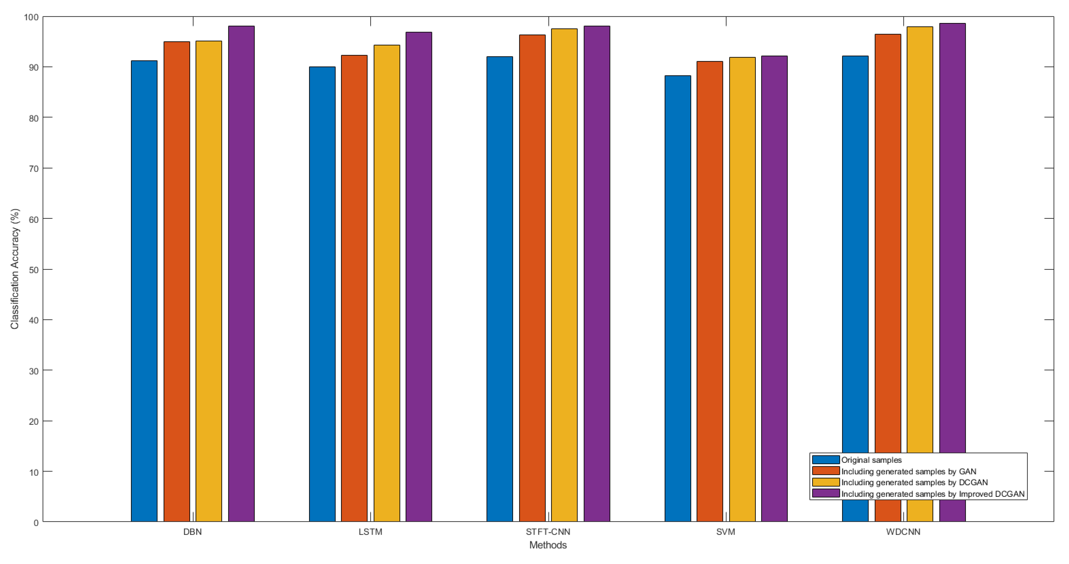
In order to verify the performance of the proposed method, the gas turbine samples are generated by GAN, DCGAN, and Improved DCGAN to form new datasets: dataset with original samples, dataset including generated samples by GAN, dataset including generated samples by DCGAN, and dataset including generated samples by Improved DCGAN. The four datasets are selected to train the classification model and classify the faults with different methods. Table 6 and Figure 18 display the classification accuracy comparisons of different diagnostic methods with the four datasets. When SVM is adopted, the classification accuracies of the dataset with original samples, the dataset including generated samples by GAN, the dataset including generated samples by DCGAN, and the dataset including generated samples by Improved DCGAN are 88.25%, 91.05%, 91.9%, and 92.15%, respectively; when LSTM is used, the classification accuracies of the four datasets are 90.05%, 92.25%, 94.3%, and 96.83%, respectively. When DBN and STFT-CNN are used, the classification results greatly improved. It can be seen that the classification effect by WDCNN performs best under each dataset compared with other methods. Meanwhile, it can be seen that the classification accuracy of the dataset with original samples, the dataset including generated samples by GAN, the dataset including generated samples by DCGAN, and dataset the including generated samples by Improved DCGAN are 92.1%, 96.4%, 97.9%, and 98.65%, respectively. It can be concluded that the classification accuracy of the dataset including generated samples by the Improved DCGAN method obviously increased compared with the dataset including generated samples by GAN and the dataset including generated samples by DCGAN.
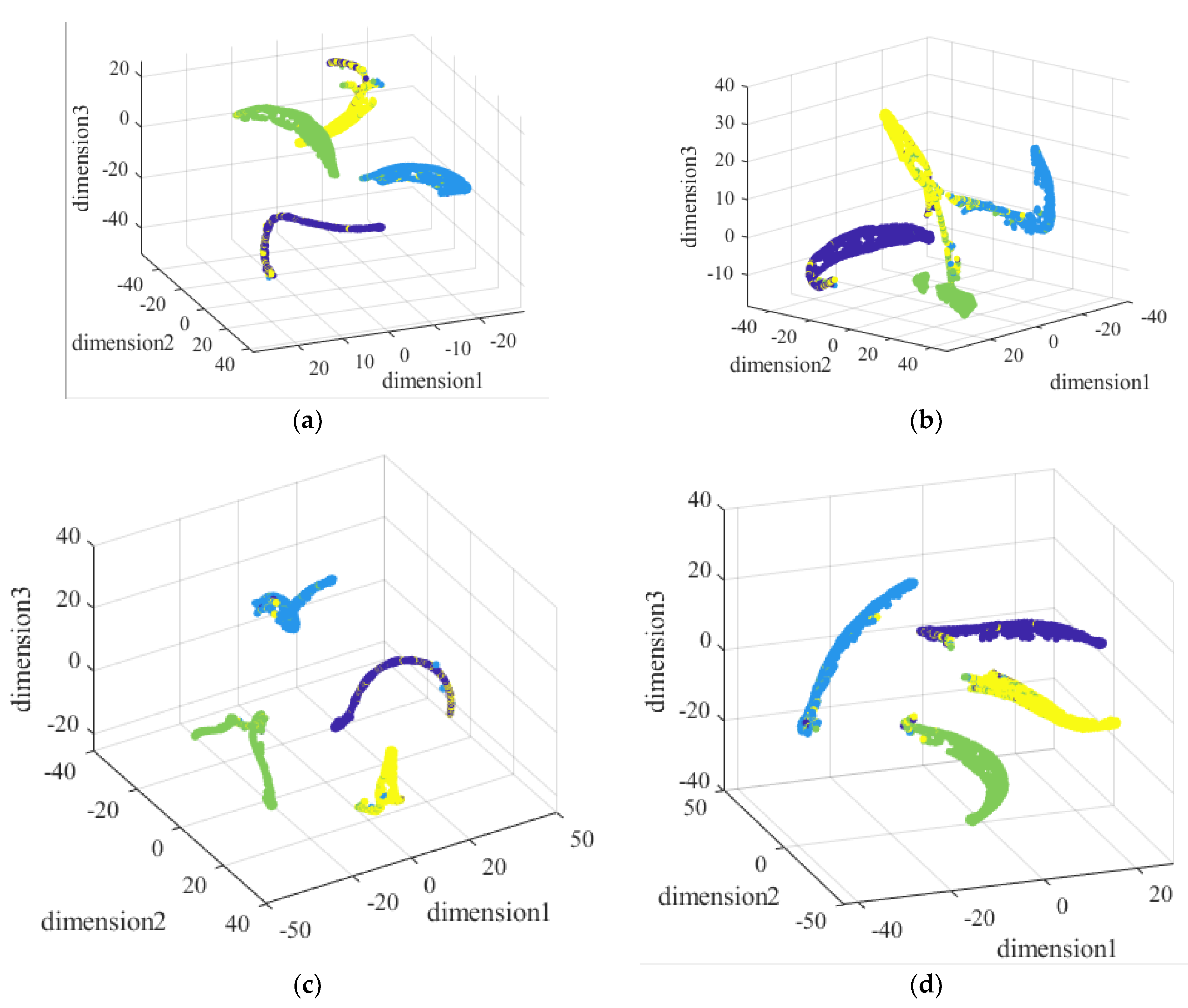
For the sake of displaying the classification results of the fault datasets by these methods, the visualized t-distributed Stochastic Neighbor Embedding (t-SNE) diagrams [51] are shown in Figure 19. Purple dots represent normal samples, blue dots represent airflow excitation fault samples, green dots are unbalanced fault samples, and yellow dots are misalignment fault samples. It can be seen in Figure 19a that the original samples without generated samples are mostly classified, unbalanced fault samples and misalignment fault samples are gathered together and not well separated, and some airflow excitation faults are misclassified. Figure 19b displays the classification results of the dataset including generated samples by GAN; it can be seen that the classification results improved. Figure 19c displays the classification results of the dataset including generated samples by DCGAN; the four types of samples are effectively separated, although some misalignment fault samples are classified as normal samples. In Figure 19d, the classification results of the proposed method are the best, with most samples classified correctly.
5. Conclusions
In this paper, a data augmentation method based on an improved Deep Convolution Generation Adversarial Network for gas turbine rotor system fault diagnosis is proposed. This method utilizes the powerful feature extraction and data generation ability of GAN to generate effective fault samples for fault diagnosis. The main highlights are summarized as follows.
Firstly, based on the Deep Convolution Generation Adversarial Network, an Improved DCGAN method combining the data generation ability of DCGAN with the feature extraction ability of WDCNN was proposed, and a new signal generator more suitable for gas turbine rotor fault signals was constructed.
Secondly, a gradient penalty was adopted to adaptively optimize the loss function according to different gas turbine rotor system faults under unknown conditions.
Finally, the effectiveness of the method was verified by gas turbine rotor system fault experiments. The results indicate that the classification accuracy improved greatly with the proposed method compared to the GAN method and the DCGAN method, and the proposed method can generate effective fault samples to solve imbalances of fault samples.
In the proposed Improved DCGAN method, the improvement of the generator makes the calculation process more complex, as it needs to be calculated by high-performance computers and this consumes more time compared with GAN and DCGAN. In further work, the attention module could be introduced to enhance the extraction of fault features. In addition, the Improved DCGAN network structure optimization could be improved to shorten the consuming time for fault diagnosis.
To sum up, the proposed method effectively supplements fault samples, solves the problem of small samples and unbalanced samples, improves the fault diagnosis accuracy, and provides an effective method and data supply for fault diagnosis of gas turbine rotor systems. Meanwhile, the method makes it more convenient for managers to understand the operation status of gas turbines, formulate the evaluation criteria of maintenance and repair, and save costs associated with suspending detection and maintenance. In the future, different sensor signals such as vibration, temperature, and flow of gas turbines can be combined for multi-source data fusion to further improve the diagnosis accuracy of gas turbines.
Author Contributions
S.L., methodology and writing; H.W., review and formal analysis; X.Z., data curation and field inspection. All authors have read and agreed to the published version of the manuscript.
Funding
This research was funded by the National Natural Science Foundation of China (No. 51975058).
Institutional Review Board Statement
Not applicable.
Informed Consent Statement
Not applicable.
Data Availability Statement
The data presented in this study are available from the corresponding author upon reasonable request.
Acknowledgments
The study was approved by the Beijing Information Science and Technology University.
Conflicts of Interest
The authors declare no conflict of interest.
References
- Zaidan, M.A.; Relan, R.; Mills, A.R.; Harrison, R.F. Prognostics of gas turbine engine: An integrated approach. Exp. Syst. Appl. 2015, 42, 8472–8483. [Google Scholar] [CrossRef]
- Ahmadi, P.; Saidi, M.H.; Dincer, I. Performance Assessment of a Hybrid Solid Oxide Fuel Cell-Gas Turbine Combined Heat and Power System. In Progress in Exergy, Energy, and the Environment; Springer International Publishing: Berlin/Heidelberg, Germany, 2014. [Google Scholar]
- Palmé, T.; Fast, M.; Thern, M. Gas turbine sensor validation through classification with artificial neural networks. Appl. Energy 2011, 88, 3898–3904. [Google Scholar] [CrossRef]
- Xia, F.; Zhang, H.; Peng, D.; Li, H.; Su, Y. Turbine fault diagnosis based on fuzzy theory and SVM. In Artificial Intelligence and Computational Intelligence; Springer International Publishing: Berlin/Heidelberg, Germany, 2009; pp. 668–676. [Google Scholar]
- Mirhosseini, A.M.; Nazari, S.A.; Pour, A.M.; Haghighi, A.E.; Zareh, M. Probabilistic failure analysis of hot gas path in a heavy-duty gas turbine using Bayesian networks. Int. J. Syst. Assur. Eng. Manag. 2019, 10, 1173–1185. [Google Scholar] [CrossRef]
- Gholamrezaei, M.; Ghorbanian, K. Application of integrated fuzzy logic and neural networks to the performance prediction of axial compressors. Proc. Inst. Mech. Eng. Part A J. Power Energy 2015, 229, 928–947. [Google Scholar] [CrossRef]
- Chen, J.; Xu, C.; Ying, Y.; Li, J.; Jin, Y.; Zhou, H.; Lin, Y.; Zhang, B. Gas-path Component Fault Diagnosis for Gas Turbine Engine: A Review. In Proceedings of the 2019 Prognostics and System Health Management Conference (PHM-Qingdao), Qingdao, China, 25–27 October 2019. [Google Scholar]
- Khaljani, M.; Saray, R.K.; Bahlouli, K. Comprehensive analysis of energy, exergy and exergo-economic of cogeneration of heat and power in a combined gas turbine and organic Rankine cycle. Energy Convers. Manag. 2015, 97, 154–165. [Google Scholar] [CrossRef]
- Amozegar, M.; Khorasani, K. An ensemble of dynamic neural network identifiers for fault detection and isolation of gas turbine engines. Neural Netw. 2016, 76, 106–121. [Google Scholar] [CrossRef]
- Buonomano, A.; Calise, F.; d’Accadia, M.D.; Palombo, A.; Vicidomini, M. Hybrid solid oxide fuel cells-gas turbine systems for combined heat and power: A review. Appl. Energy 2015, 156, 32–85. [Google Scholar] [CrossRef]
- Zhang, J.; Ma, W.; Lin, J.; Ma, L.; Jia, X. Fault diagnosis approach for rotating machinery based on dynamic model and computational intelligence. Measurement 2015, 59, 73–87. [Google Scholar] [CrossRef]
- Shao, H.; Jiang, H.; Zhao, H.; Wang, F. A novel deep autoencoder feature learning method for rotating machinery fault diagnosis. Mech. Syst. Signal Process. 2017, 95, 187–204. [Google Scholar] [CrossRef]
- Sun, H.; He, Z.; Zi, Y.; Yuan, J.; Wang, X.; Chen, J.; He, S. Multiwavelet transform and its applications in mechanical fault diagnosis—A review. Mech. Syst. Signal Process. 2014, 43, 1–24. [Google Scholar] [CrossRef]
- Cabal-Yepez, E.; Garcia-Ramirez, A.G.; Romero-Troncoso, R.J.; Garcia-Perez, A.; Osornio-Rios, R.A. Reconfigurable monitoring system for time-frequency analysis on industrial equipment through STFT and DWT. IEEE Trans. Ind. Inform. 2013, 9, 760–771. [Google Scholar] [CrossRef]
- Mohammadi, E.; Montazeri-Gh, M. A fuzzy-based gas turbine fault detection and identification system for full and part-load performance deterioration. Aerosp. Sci. Technol. 2015, 46, 82–93. [Google Scholar] [CrossRef]
- Hanachi, H.; Mechefske, C.; Liu, J.; Banerjee, A.; Chen, Y. Performance-Based Gas Turbine Health Monitoring, Diagnostics, and Prognostics: A Survey. IEEE Trans. Reliab. 2018, 67, 1340–1363. [Google Scholar] [CrossRef]
- Attarian, M.; Molaei, S.; Shokri, H.; Norouzi, K. Failure and Metallurgical Defects Analysis of IN-738LC Gas Turbine Blades. Eng. Fail. Anal. 2021, 122, 105213. [Google Scholar] [CrossRef]
- Tahan, M.; Muhammad, M.; Karim, Z.A. A multi-nets ANN model for real-time performance-based automatic fault diagnosis of industrial gas turbine engines. J. Braz. Soc. Mech. Sci. Eng. 2017, 39, 2865–2876. [Google Scholar] [CrossRef]
- Saidi, L.; Ali, J.B.; Fnaiech, F. Application of higher order spectral features and support vector machines for bearing faults classification. ISA Trans. 2015, 54, 193–206. [Google Scholar] [CrossRef] [PubMed]
- Gayme, D.; Menon, S.; Ball, C.; Mukavetz, D.; Nwadiogbu, E. Fault diagnosis in gas turbine engines using fuzzy logic. In Proceedings of the 2003 IEEE International Conference on Systems, Man and Cybernetics, Conference Theme—System Security and Assurance (Cat. No.03CH37483), Washington, DC, USA, 8 October 2003; pp. 3756–3762. [Google Scholar]
- Wang, H.; Du, W. A new K-means singular value decomposition method based on self-adaptive matching pursuit and its application in fault diagnosis of rolling bearing weak fault. Int. J. Distrib. Sens. Netw. 2020, 16, 1–12. [Google Scholar] [CrossRef]
- Rahmoune, M.B.; Hafaifa, A.; Kouzou, A.; Chen, X.; Chaibet, A. Gas turbine monitoring using neural network dynamic nonlinear autoregressive with external exogenous input modelling. Math. Comput. Simul. 2021, 179, 23–47. [Google Scholar] [CrossRef]
- Rao, A.; Satish, T.N.; Nambiar, A.S.; Jana, S.; Naidu, V.P.S.; Uma, G.; Umapathy, M. Challenges in Engine Health Monitoring Instrumentation during Developmental Testing of Gas Turbine Engines. In Proceedings of the National Aerospace Propulsion Conference; Springer: Berlin/Heidelberg, Germany, 2020. [Google Scholar]
- Yang, X.; Bai, M.; Liu, J.; Liu, J.; Yu, D. Gas path fault diagnosis for gas turbine group based on deep transfer learning. Measurement 2021, 181, 109631. [Google Scholar] [CrossRef]
- Karri, S.P.K.; Chakraborty, D.; Chatterjee, J. Transfer learning based classification of optical coherence tomography images with diabetic macular edema and dry age-related macular degeneration. Biomed. Optics Express 2017, 8, 579. [Google Scholar] [CrossRef] [Green Version]
- Xiao, D.; Huang, Y.; Qin, C.; Liu, Z. Transfer learning with convolutional neural networks for small sample size problem in machinery fault diagnosis. Proc. Inst. Mech. Eng. Part C J. Mech. Eng. Sci. 2019, 233, 5131–5143. [Google Scholar] [CrossRef]
- Zhao, Y.; Xu, G.; Liu, M. Method for fault diagnosis of bearing based on transfer learning with VGG16 model. Spacecr. Environ. Eng. 2020, 37, 6. [Google Scholar]
- Liu, S.; Jiang, H.; Wu, Z.; Li, X. Data synthesis using deep feature enhanced generative adversarial networks for rolling bearing imbalanced fault diagnosis. Mech. Syst. Signal Proc. 2022, 163, 108139. [Google Scholar] [CrossRef]
- Bharti, V.; Biswas, B.; Shukla, K.K. EMOCGAN: A novel evolutionary multiobjective cyclic generative adversarial network and its application to unpaired image translation. Neural Comput. Appl. 2021, 1–15. [Google Scholar] [CrossRef]
- Luo, J.; Huang, J.; Li, H. A case study of conditional deep convolutional generative adversarial networks in machine fault diagnosis. J. Intell. Manuf. 2021, 32, 407–425. [Google Scholar] [CrossRef]
- Wang, R.; Zhang, S.; Chen, Z.; Li, W. Enhanced generative adversarial network for extremely imbalanced fault diagnosis of rotating machine. Measurement 2021, 180, 109467. [Google Scholar] [CrossRef]
- Viola, J.; Chen, Y.Q.; Wang, J. FaultFace: Deep Convolutional Generative Adversarial Network (DCGAN) based Ball-Bearing Failure Detection Method. Inf. Sci. 2021, 542, 195–211. [Google Scholar] [CrossRef]
- Li, Q.; Chen, L.; Shen, C.; Yang, B. Enhanced generative adversarial networks for fault diagnosis of rotating machinery with imbalanced data. Meas. Sci. Technol. 2019, 30, 115005. [Google Scholar] [CrossRef]
- Wu, Q.; Chen, Y.; Meng, J. DCGAN Based Data Augmentation for Tomato Leaf Disease Identification. IEEE Access 2020, 8, 98716–98728. [Google Scholar] [CrossRef]
- Wang, F.; Jiang, H.; Shao, H.; Duan, W.; Wu, S. An adaptive deep convolutional neural network for rolling bearing fault diagnosis. Meas. Sci. Technol. 2017, 28, 095005. [Google Scholar]
- Dewi, C.; Chen, R.C.; Liu, Y.T.; Tai, S.-K. Synthetic Data generation using DCGAN for improved traffic sign recognition. Neural Comput. App. 2021, 1–16. [Google Scholar] [CrossRef]
- Li, J.; Zhao, B.; Wu, K.; Dong, Z.; Zhang, X.; Zheng, Z. A Representation Generation Approach of Transmission Gear Based on Conditional Generative Adversarial Network. Actuators 2021, 10, 86. [Google Scholar] [CrossRef]
- Awan, S.E.; Bennamoun, M.; Sohel, F.; Sanfilippo, F.; Dwivedi, G. Imputation of Missing Data with Class Imbalance using Conditional Generative Adversarial Networks. Neurocomputing 2021, 453, 164–171. [Google Scholar] [CrossRef]
- He, W.; He, Y.; Li, B. Generative Adversarial Networks with Comprehensive Wavelet Feature for Fault Diagnosis of Analog Circuits. IEEE Trans. Instrum. Meas. 2020, 69, 6640–6650. [Google Scholar] [CrossRef]
- Radford, A.; Metz, L.; Chintala, S. Unsupervised representation learning with deep convolutional generative adversarial networks. arXiv 2015, arXiv:1511.06434. [Google Scholar]
- Yu, J.; Guo, Z. Remaining useful life prediction of planet bearings based on conditional deep recurrent generative adversarial network and action discovery. J. Mech. Sci. Technol. 2021, 35, 21–30. [Google Scholar] [CrossRef]
- Zhu, M.; Zhang, Z.; Mei, J.; Zhou, K.; Chen, P.; Qi, Y.; Huang, Q. Data Augmentation Using DCGAN for Improved Fault Detection of High Voltage Shunt Reactor. J. Phys. Conf. Ser. 2021, 1944, 012012. [Google Scholar] [CrossRef]
- Shao, S.; McAleer, S.; Yan, R.; Baldi, P. Highly accurate machine fault diagnosis using deep transfer learning. IEEE Trans. Ind. Inform. 2019, 15, 2446–2455. [Google Scholar] [CrossRef]
- Chen, Z.Q.; Li, C.; Sanchez, R.V. Gearbox fault identification and classification with convolutional neural networks. Shock Vib. 2015, 2015, 390134. [Google Scholar] [CrossRef] [Green Version]
- Jia, X.; Zhao, M.; Di, Y.; Yang, Q.; Lee, J. Assessment of Data Suitability for Machine Prognosis Using Maximum Mean Discrepancy. IEEE Trans. Ind. Electron. 2017, 65, 5872–5881. [Google Scholar] [CrossRef]
- Mao, W.; Chen, J.; Chen, Y.; Afshari, S.S.; Liang, X. Construction of Health Indicators for Rotating Machinery Using Deep Transfer Learning with Multiscale Feature Representation. IEEE Trans. Instrum. Meas. 2021, 70, 3511313. [Google Scholar] [CrossRef]
- Imbalanced Fault Classification of Bearing via Wasserstein Generative Adversarial Networks with Gradient Penalty. Shock Vib. 2020, 2020, 8836477.
- Hashemizadehkolowri, S.K.; Chen, R.R.; Adluru, G.; Dean, D.C.; Wilde, E.A.; Alexander, A.L.; DiBella, E.V.R. Simultaneous multi-slice image reconstruction using regularized image domain split slice-GRAPPA for diffusion MRI. Med. Image Anal. 2021, 70, 102000. [Google Scholar] [CrossRef] [PubMed]
- Shao, H.; Jiang, H.; Zhang, X.; Niu, M. Rolling bearing fault diagnosis using an optimization deep belief network. Meas. Sci. Technol. 2015, 26, 115002. [Google Scholar] [CrossRef]
- Ravikumar, K.N.; Yadav, A.; Kumar, H.; Gangadharan, K.V.; Narasimhadhan, A.V. Gearbox Fault Diagnosis based on Multi-Scale Deep Residual Learning and Stacked LSTM Model. Measurement 2021, 186, 110099. [Google Scholar] [CrossRef]
- Zhao, K.; Jiang, H.; Wu, Z.; Lu, T. A novel transfer learning fault diagnosis method based on Manifold Embedded Distribution Alignment with a little labeled data. J. Intell. Manuf. 2020, 33, 151–165. [Google Scholar] [CrossRef]
Figure 1.
GAN network structure diagram.

Figure 2.
Structure of DCGAN.

Figure 3.
Structure of Improved DCGAN.

Figure 4.
Flow chart of the proposed gas turbine rotor fault diagnosis method.

Figure 5.
Schematic diagram of gas turbine vibration test.

Figure 6.
Gas turbine vibration signals at front measuring point.

Figure 7.
RMS for gas turbine vibration signals.

Figure 8.
Different vibration signals for gas turbine rotor system faults. (a) Normal state. (b) Airflow excitation. (c) Unbalanced. (d) Misalignment.
Figure 8.
Different vibration signals for gas turbine rotor system faults. (a) Normal state. (b) Airflow excitation. (c) Unbalanced. (d) Misalignment.

Figure 9.
Time–frequency analysis of gas turbine rotor faults. (a) Misalignment. (b) Unbalanced.

Figure 10.
The fatigue damage of the shaft.

Figure 11.
Fatigue crack of blade.

Figure 12.
Fault data generation and classification of gas turbine rotor system.

Figure 13.
Loss function of generator and discriminator.

Figure 14.
Signal comparison of time domain and frequency domain of the original signals and the generated signals in normal state.
Figure 14.
Signal comparison of time domain and frequency domain of the original signals and the generated signals in normal state.

Figure 15.
Signal comparison of time domain and frequency domain of the original signals and the generated signals in airflow excitation state.
Figure 15.
Signal comparison of time domain and frequency domain of the original signals and the generated signals in airflow excitation state.

Figure 16.
Signal comparison of time domain and frequency domain of the original signals and the generated signals in unbalanced state.
Figure 16.
Signal comparison of time domain and frequency domain of the original signals and the generated signals in unbalanced state.

Figure 17.
Signal comparison of time domain and frequency domain of the original signals and the generated signals in misalignment state.
Figure 17.
Signal comparison of time domain and frequency domain of the original signals and the generated signals in misalignment state.

Figure 18.
Comparisons of classification results.

Figure 19.
Accuracy comparisons with different datasets. (a) Original samples. (b) Including generated samples by GAN. (c) Including generated samples by DCGAN. (d) Including generated samples by Improved DCGAN.
Figure 19.
Accuracy comparisons with different datasets. (a) Original samples. (b) Including generated samples by GAN. (c) Including generated samples by DCGAN. (d) Including generated samples by Improved DCGAN.


Table 1.
Detailed settings of the WDCNN structure.
| Layer Type | Activation | Kernel Number | Kernel Size × Stride | Output Size |
|---|---|---|---|---|
| Input | (1024, 1) | |||
| Conv1 | ReLU | 20 | 32 × 8 | 125 × 1 × 20 |
| BN | 125 × 1 × 20 | |||
| Pool | 20 | 2 × 2 | 62 × 1 × 20 | |
| Conv | ReLU | 20 | 3 × 1 | 62 × 1 × 20 |
| BN | 62 × 1 × 20 | |||
| Pool | 20 | 2 × 2 | 31 × 1 × 20 | |
| Conv | ReLU | 20 | 3 × 1 | 31 × 1 × 20 |
| BN | 31 × 1 × 20 | |||
| Pool | 20 | 2 × 2 | 15 × 1 × 20 | |
| Conv | ReLU | 20 | 3 × 1 | 15 × 1 × 20 |
| BN | 15 × 1 × 20 | |||
| Pool | 20 | 2 × 2 | 7 × 1 × 20 | |
| FC1 | 1 × 1 × 1024 | |||
| FC2 | 1 × 1 × 4 |
Table 2.
Structure parameters and hyper-parameters of Improved DCGAN.
| Model | Network Layer | Kernel Size | Stride | Activation Function | Kernel Number |
|---|---|---|---|---|---|
| Generator | Conv1 | 32 | 8 | ReLU | 20 |
| Conv2 | 3 | 1 | ReLU | 20 | |
| Conv3 | 3 | 1 | ReLU | 40 | |
| Conv4 | 3 | 1 | ReLU | 40 | |
| Deconv1 | 3 | 1 | ReLU | 128 | |
| Deconv2 | 3 | 2 | ReLU | 64 | |
| Deconv3 | 3 | 2 | ReLU | 32 | |
| Deconv4 | 3 | 2 | Tanh | 1 | |
| Discriminator | Conv1 | 3 | 2 | LeakReLU | 32 |
| Conv2 | 3 | 2 | LeakReLU | 64 | |
| Conv3 | 3 | 2 | LeakReLU | 128 | |
| Conv4 | 3 | 2 | LeakReLU | 256 | |
| Conv5 | 2 | 1 | 1 |
Table 3.
Number of training dataset and testing dataset samples.
| No. | Class | Number of Samples in Original Training Dataset (Labeled) | Number of Samples in Training Dataset Including Generated Samples (Labeled) | Number of Samples in Testing Dataset (Unlabeled) |
|---|---|---|---|---|
| 1 | Normal | 600 | 1000 | 500 |
| 2 | Airflow excitation | 500 | 1000 | 500 |
| 3 | Unbalanced | 500 | 1000 | 500 |
| 4 | Misalignment | 500 | 1000 | 500 |
Table 4.
SSIM comparisons on between generated signals and real signals under different states.
| Faults | STFT | CWT | ||||
|---|---|---|---|---|---|---|
| GAN | DCGAN | Improved DCGAN | GAN | DCGAN | Improved DCGAN | |
| Normal | 0.8699 | 0.9502 | 0.9937 | 0.7884 | 0.9456 | 0.9660 |
| Airflow excitation | 0.8522 | 0.9482 | 0.9937 | 0.7874 | 0.9368 | 0.9885 |
| Unbalanced | 0.8576 | 0.9403 | 0.9955 | 0.7959 | 0.9345 | 0.9683 |
| Misalignment | 0.8412 | 0.9214 | 0.9944 | 0.7976 | 0.9421 | 0.9683 |
Table 5.
Comparison of different diagnostic models.
| Method | Precision | Accuracy | |||
|---|---|---|---|---|---|
| Normal | Airflow Excitation | Unbalanced | Misalignment | ||
| DBN | 98.90% | 98.40% | 97.80% | 97.00% | 98.03% |
| SVM | 92.50% | 94.60% | 90.30% | 91.30% | 92.15% |
| STFT-CNN | 97.30% | 97.80% | 98.40% | 98.80% | 98.08% |
| WDCNN | 99.80% | 98.10% | 98.30% | 98.40% | 98.65% |
| LSTM | 96.80% | 98.60% | 93.20% | 98.70% | 96.83% |
Table 6.
Comparison of different diagnostic methods for different datasets.
| Method | Accuracy for Different Datasets | |||
|---|---|---|---|---|
| Original Samples | Including Generated Samples by GAN | Including Generated Samples by DCGAN | Including Generated Samples by Improved DCGAN | |
| SVM | 88.25% | 91.05% | 91.90% | 92.15% |
| LSTM | 90.05% | 92.25% | 94.30% | 96.83% |
| DBN | 91.25% | 94.95% | 95.15% | 98.03% |
| STFT-CNN | 91.95% | 96.25% | 97.45% | 98.08% |
| WDCNN | 92.10% | 96.40% | 97.90% | 98.65% |
Publisher’s Note: MDPI stays neutral with regard to jurisdictional claims in published maps and institutional affiliations. |
© 2022 by the authors. Licensee MDPI, Basel, Switzerland. This article is an open access article distributed under the terms and conditions of the Creative Commons Attribution (CC BY) license (https://creativecommons.org/licenses/by/4.0/).
Share and Cite
MDPI and ACS Style
Liu, S.; Wang, H.; Zhang, X. Research on Improved Deep Convolutional Generative Adversarial Networks for Insufficient Samples of Gas Turbine Rotor System Fault Diagnosis. Appl. Sci. 2022, 12, 3606. https://doi.org/10.3390/app12073606
AMA Style
Liu S, Wang H, Zhang X. Research on Improved Deep Convolutional Generative Adversarial Networks for Insufficient Samples of Gas Turbine Rotor System Fault Diagnosis. Applied Sciences. 2022; 12(7):3606. https://doi.org/10.3390/app12073606
Chicago/Turabian StyleLiu, Shucong, Hongjun Wang, and Xiang Zhang. 2022. "Research on Improved Deep Convolutional Generative Adversarial Networks for Insufficient Samples of Gas Turbine Rotor System Fault Diagnosis" Applied Sciences 12, no. 7: 3606. https://doi.org/10.3390/app12073606
Note that from the first issue of 2016, this journal uses article numbers instead of page numbers. See further details here.