
Correlations and Asymptotic Behaviors of the Shape Parameters of Floating Bubbles Using an Improved Numerical Procedure

Department of Mechanical Engineering, Kunsan National University, Gunsan 54150, Korea
Appl. Sci. 2022, 12(4), 1804; https://doi.org/10.3390/app12041804
Submission received: 19 December 2021
/
Revised: 25 January 2022
/
Accepted: 7 February 2022
/
Published: 9 February 2022
(This article belongs to the Section Fluid Science and Technology)
Abstract
:An improved numerical procedure is used to present the correlations between the shape parameters and Bond numbers of floating bubbles for a wider range of Bond numbers () than the previously reported range of Bond numbers (, and their asymptotic relations as Bo → 0 and Bo → ∞. The proposed method is proven to be more precise and robust than the conventional methods in comparison with previous numerical and experimental results. In addition, the profile of floating bubbles and the related parameters are presented for a wide range of bubble sizes. The shape parameters are divided into three distinct Bond number regions, and are fitted with a fifth-order polynomial as a function of Bond number on a log-log scale for each region. The parameters show two asymptotes, which can be expressed in a simple power law. In addition, the dimensionless maximum depth of the floating bubble is obtained as when . These correlations and asymptotic relations are expected to assist in the development of scale models of dynamic bubble-related phenomena such as bubble bursting.
1. Introduction
Bubbles floating on a liquid can be seen in various places, and an understanding of the related phenomena is important in the natural sciences and industrial fields. For example, the bursting of floating bubbles in the ocean affects atmospheric circulation and marine pollution [1,2,3,4]. In a nuclear power plant accident, the bursting of bubbles in the reactor acts as a source of radionuclides [5,6]. Volcanic eruptions are caused by bubbles with sizes measured in meters [7]. In food engineering, bubbles are involved in the release of foams and flavors, e.g., champagne, espresso, and beer [8,9,10,11]. Recently, boiling heat transfer in a complex nanofluid is closely related to bubble nucleation and growth [12,13].
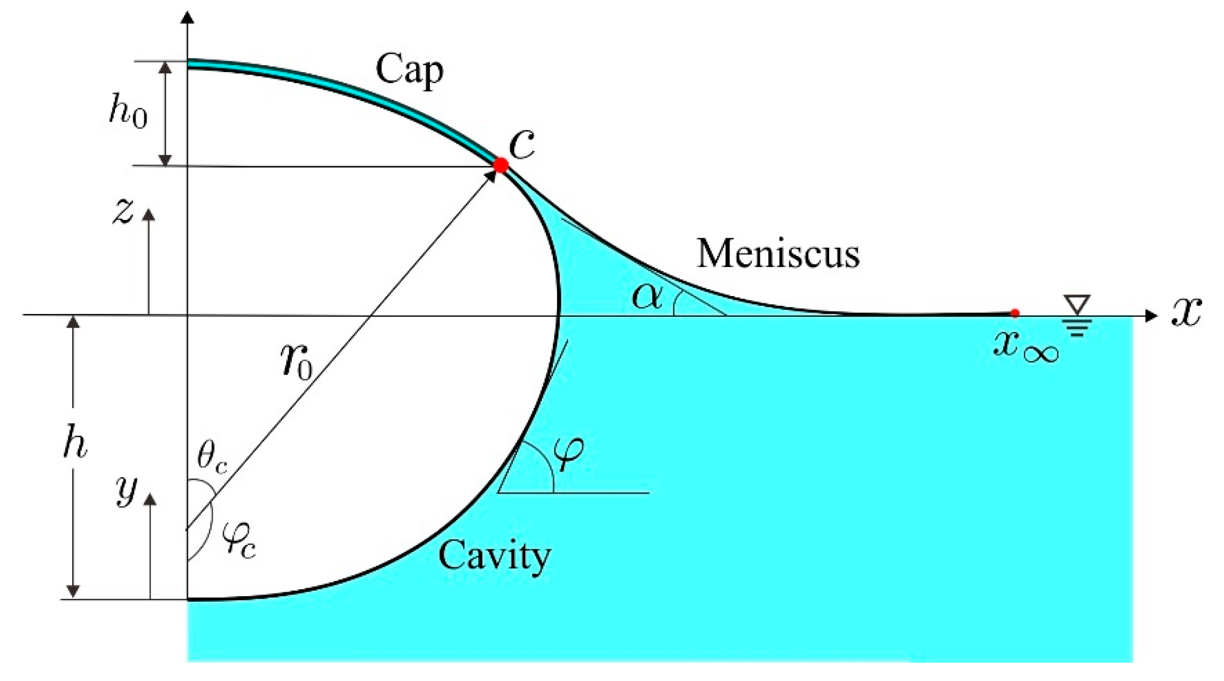
Bubbles generated in a liquid rise due to buoyancy, and then burst after reaching the liquid surface [14]. Bubbles floating on a liquid can remain in quasi-equilibrium for some time before bursting. During this time, the thin liquid film that defines the surface of the bubble gradually becomes thinner and unstable due to gravity, external disturbance, and impurities [15]. After bursting, the dynamics of the bubble cannot be simulated by the present numerical method, and the partial differential equations of the conservation laws must be solved using the computational fluid dynamics techniques such as the finite element method [16], the arbitrary Lagrangian–Eulerian moving mesh method [17], the two-fluid two-phase flow model [18,19], and the adaptive multi-phase method [20]. As shown schematically in Figure 1, the shape of the floating bubbles in the quasi-equilibrium state can be divided into three curves, namely the cap, the cavity, and the meniscus. These three curves meet at a junction point . As the various dynamic phenomena that occur when a floating bubble bursts depend largely on its initial shape, the accurate prediction of this shape is important [21,22,23,24,25,26,27]. If the thickness and drainage of the liquid film can be neglected, then the shape of the bubble in the quasi-equilibrium state is determined by the Young–Laplace equation representing the balance between the forces of hydrostatic pressure and capillary action [28,29,30,31,32]. Floating bubbles vary in shape from spherical to hemispherical, depending on their size. Therefore, the Bond number, , is used as a key parameter.
Bashforth and Adams [28] presented a systematic theoretical equation for hydrostatic pressure and capillary forces and obtained a series solution of drops of fluids. Subsequently, Toba [29] calculated the shapes of floating bubbles by using a semi-graphical method. At the same time, Princen [30] used the Table of Bashforth and Adams [28] to find the junction point and calculate the shapes of bubbles of various sizes. Medrow and Chao [31] numerically calculated the bubble shape for a broader range of the bubble sizes (which corresponds to a range of , computed based on the parameter values of [31]), and derived an analytic solution using a perturbation technique for tiny bubbles that are difficult to calculate numerically. Recently, Lhuissier and Villermaux [23] obtained the bubble shape via a method similar to that of Toba [29]; however, there is no detailed information on their numerical method and on the accuracy of their solution. Bartlett [32] used a similar method to Princen [30] and presented the shapes of bubbles for Bond numbers between 0.1 to 100. Cohen et al. [33] developed a model considering the film weight of giant soap bubbles and compared the results of numerical solutions and experiments. Shaw and Deike [34] studied the coalescence of floating bubbles for a wide range of Bond number, and characterized the evolution of the underwater neck and the surface bridge. Miguet et al. [35] investigated the life of a floating bubble by exploring the role of drainage and evaporation on film thinning. Despite a long period of study, the bubble sizes used for analysis have been limited, and there is no rigorous evaluation of the accuracy and robustness of the numerical methods used.
As bubble shape parameters play an important role in the theory describing various dynamic phenomena related to floating bubbles [36], accurate prediction of the bubble parameter is crucial, especially in a wide range of Bond numbers. For instance, the lifetimes of floating bubbles are related to the surface area of the bubble film [15]. The jet velocity generated when the bubble bursts is related to the depth of the cavity, and the amount of aerosol emitted depends on the radius and height of the cap [23,27]. Koch et al. [5] used the correlation between the dimensionless cap area and the dimensionless diameter to calculate the number of film droplets generated in the bubble bursting process, and the correlation between the dimensionless base radius and the dimensionless diameter to obtain the critical film thickness. Teixeira et al. [37] employed a perturbation method for large bubbles to obtain analytical expressions for bubble parameters as a function of the Bond number, and compared their results with experimental data. Puthenveettil et al. [36] also derived approximate analytical solutions for bubble parameters over a moderate range of Bond number () and compared these with their experimental results. Moreover, to the best of the present author’s knowledge, no study has yet been published detailing the correlations between the Bond number and various bubble parameters over an extensive range of Bond numbers.
In the present work, an improved numerical procedure is proposed to calculate the shapes of floating bubbles over a much wider range of Bond numbers than that examined in the previous studies. The proposed method is validated against the earlier numerical and experimental results to prove its accuracy and robustness. New correlations between the Bond number and several important bubble parameters, along with their asymptotic relations, are then provided.
The novelty of this study is as follows. A new method is developed by introducing specific functions for accurately finding the location of the connection points on the bubble surface regardless of the ODE solvers and their boundary points. An improved algorithm to find the junction point is developed, based on a novel function to determine the type of meniscus.
2. Theoretical Model
A slightly modified form of the theoretical model presented by Toba [29] and Medrow and Chao [31] is used in the present work. Thus, the shape of the floating bubble is described by the Young–Laplace equation:
where is the pressure difference across the interface, is the surface tension, and and are the principal radii of curvature.
A half-section of an axisymmetric bubble floating on a liquid is presented, along with its associated parameters, in Figure 1, where is the depth of the cavity below the undisturbed liquid surface, is the point where the meniscus meets the undisturbed surface, and and are the tangent angles of the cavity and meniscus curves, respectively.
If the thickness of the cap film is ignored, then the cap has a spherical shape with a radius , and Equation (1) can be written as
where denotes the pressure difference across the cap film. Furthermore, if the weight of gas inside the bubble is neglected, then the cavity satisfies
where and denote the liquid density and gravitational acceleration, respectively,
Similarly, the meniscus shape is given by
As the bubble shape is a surface of revolution about the z-axis, the principal radii of curvature are given as
By using the capillary length, , the bubble parameters are nondimensionalized as given by
Substituting Equations (2) and (5)–(7) into Equation (3) yields the dimensionless ordinary differential equations (ODEs) for the cavity shape, given here as
where the parameter represents the dimensionless pressure difference across the bottom of the bubble, as defined by
Equations (8) and (9) can be rewritten with an independent variable as
Application of the L’Hospital’s rule, i.e., , then leads to the first initial condition of Equations (8) as follows:
The second initial condition of Equation (9) is simply given as
Similarly, the relation is used to obtain the ODEs for the meniscus shape as follows:
The boundary conditions of Equations (15) and (16) at are given as
At the junction point , the geometrical relationship given in Equation (18) must be satisfied:
From Equations (10) and (18), the relation between and is given as
As the cap is spherical with a radius , its shape is given by
The volume of the bubble is computed analytically via integration by parts [38]. The volume of the cap is given by
where .
The volume of the cavity is given by
The surface area of the cap is obtained as
However, there is no analytic form for the surface area of the cavity. It should be numerically integrated as follows:
where and respectively denote the X and Y positions on the cavity at .
The Bond number is defined by
where denotes the equivalent spherical radius of the bubble.
3. Numerical Procedure
Given the parameter , the shape of the floating bubble can be determined. Since the bubble is symmetric about the z-axis, only half of it is needed. First, the shape of the cavity shape between the bottom and the junction point is calculated, then the shape of the meniscus between the point and the boundary point is determined. Finally, the shape of the circular cap is quickly obtained. The junction point between the cavity and the meniscus is not given analytically and should be found via a numerical iterative method. The accuracy of the bubble shape is significantly affected by the accuracy with which is located.
The dimensionless height is used to determine whether the guessed junction point matches the exact point . Given the position of , is readily calculated from Equation (19). Furthermore, after computing the meniscus shape, another height, , can be obtained. Thus, the bubble shape is considered to have converged when the error falls within a defined level of tolerance that indicates the accuracy of the numerical method used.
3.1. Improving the Accuracy of the Cavity Shape
The cavity shape can be obtained by integrating Equations (8) and (9) or Equations (11) and (12) numerically. However, previous studies have shown that it is necessary to divide the cavity into two [29,32,39] or three [31] parts in order to avoid divergence of Equations (8) and (9) at . In the present study, when the cavity was divided into two parts, the numerical error was found to increase rapidly as the bubble size decreased (see Figure 6). Hence, the cavity shape was divided into the following three parts or intervals: (I) , (II) , and (III) , and Equations (8) and (9) were applied to intervals (I) and (III), while Equations (11) and (12) were applied to interval (II). However, because is not an independent variable in these equations, the numerical integrations are not completely finished at and . Hence, a conventional method is to set an arbitrary far point (or ) as a boundary condition of the ODEs and to finish the calculation when is just greater than (or ). Unfortunately, this leads to potential errors at the endpoint (or ) of the divided cavity depending on ODE solvers. The conventional method works well on medium-sized bubbles, but produces a severe error in large bubbles, especially at the position of , because the bottom of the cavity becomes substantially flat. This error is not only affected by the boundary points (or ), but also by the tolerance of the ODE solver.
To remedy this problem, an improved method was proposed for accurately finding the location of the connection points and regardless of the ODE solvers and their boundary points. In this approach, a monotonically increasing function is defined as follows:
| function |
| to to find at the endpoint |
| return |
| end function |
An accurate position is then found by solving in the interval using a root-finding technique. Here, the boundary point is any value greater than ; usually, is appropriate for most of the bubble sizes considered in this study. As shown in Figure 2b, does not affect the accuracy of the solution obtained using this method at all. Once has been determined, Equations (8) and (9) are integrated again from to to obtain the first part of the cavity profile along with the remaining and . Similarly, the second part of the cavity and its endpoint can be computed using the following function:
| function |
| to to find at the endpoint |
| return |
| endfunction |
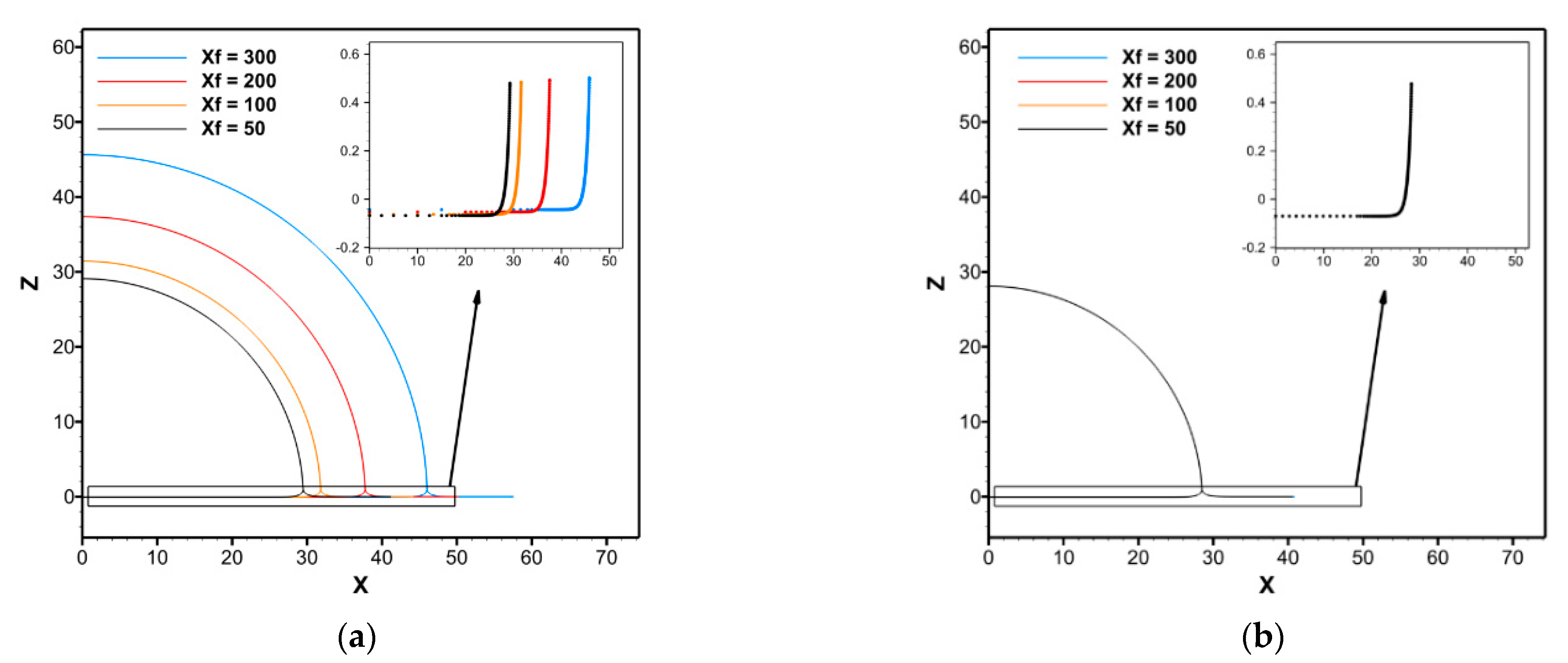
The computed bubble shapes according to the position of the boundary point for a large bubble () are presented in Figure 2. Here, the bubble shapes are seen to vary significantly depending on when the conventional technique is used (Figure 2a). When the root-finding method is used, however, the bubble shapes not affected by (Figure 2b).
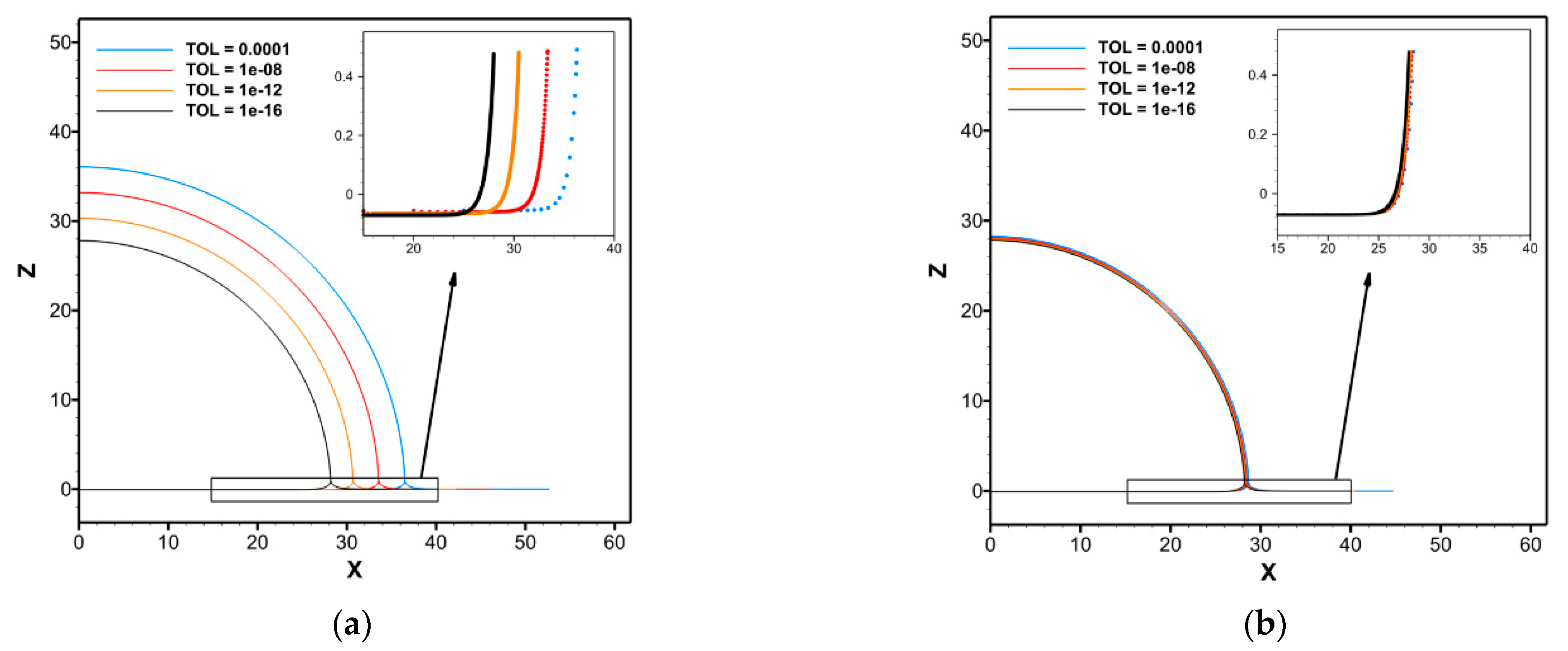
Similarly, the effect of ODE solver tolerances for the same size of bubble are presented in Figure 3. Here, the bubble shape changes slightly according to the tolerance using the improved method (Figure 3b), but the results obtained using the conventional method are unacceptable (Figure 3a). Therefore, it is essential to compute the connection point accurately for large bubbles.
3.2. Finding the Junction Point Based on the Type of Meniscus
There are two general approaches to finding the junction point according to the direction of integration of the meniscus. The first approach is to integrate the meniscus from to in the negative X-direction [29,31]. Here, is sought in an iterative manner so that the derivatives of the meniscus and cavity profiles match at the junction point . However, it is difficult to compute the shape of the meniscus using this method because the initial slope becomes zero when the exact initial condition, at , is applied. To circumvent this, Toba [29] and Freud and Freud [40] employed at as an initial condition. Medrow and Chao [31] further improved this method by using an approximate analytical solution of with the Bessel function. Nevertheless, as these methods do not give an exact initial condition at , the accuracy of the solution is still limited.
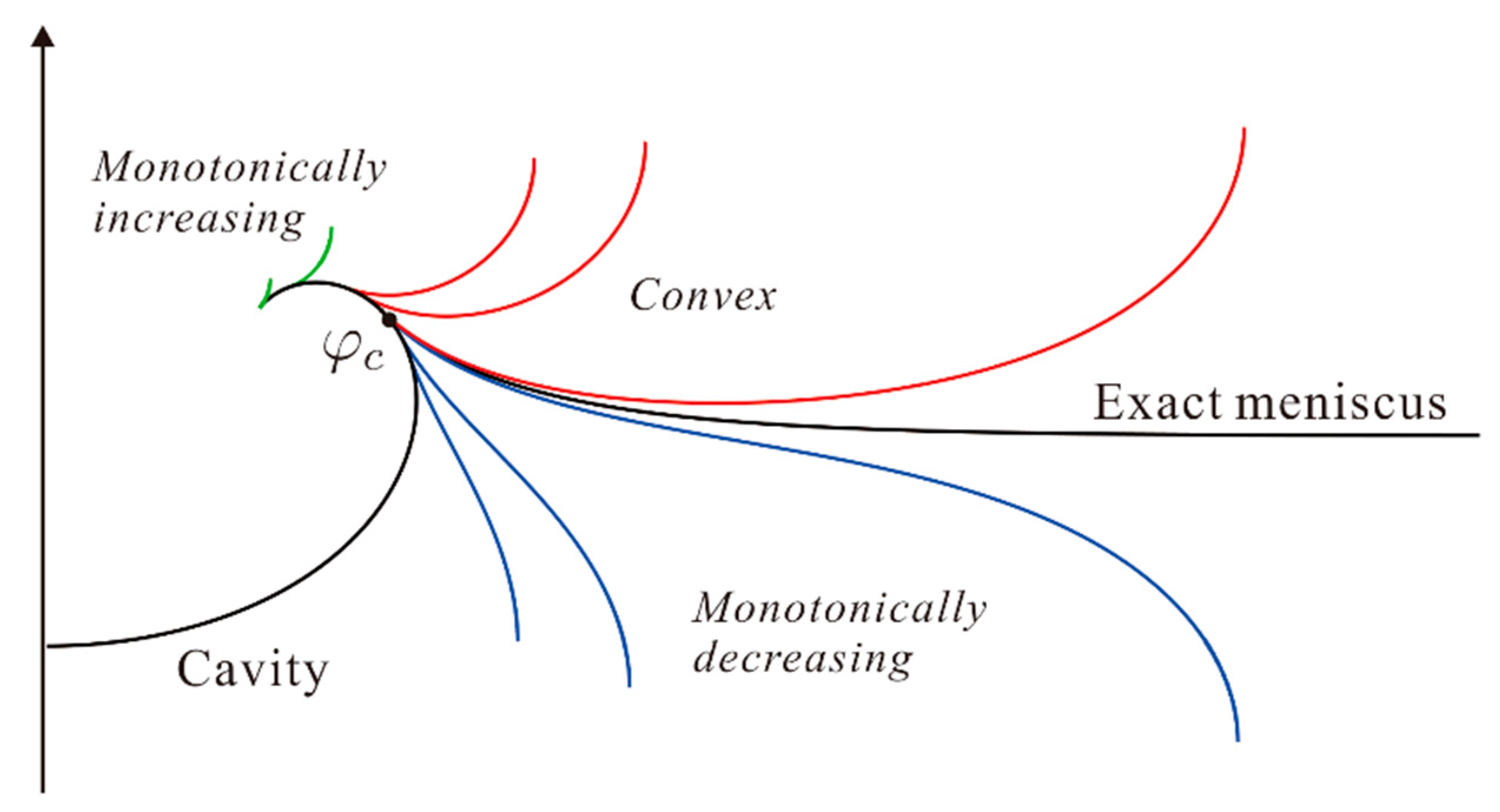
The second approach is to integrate the meniscus from to in the positive X-direction [23,30,32]. Although this approach has the advantage of obtaining the position more precisely, there is another difficulty in that the meniscus shape changes dramatically around the junction point , as shown in Figure 4.
Hence, a method for effectively locating the junction point is proposed herein by using a specific function that distinguishes the type of meniscus shape. A conventional bisection method for finding narrows the interval by comparing the sign of at both ends of the solution interval. At each iteration step, it is necessary to find the height , which is calculated differently depending on the meniscus type: if the meniscus profile is convex, its minimum value is chosen; if the meniscus profile is monotonically decreasing, an inflection point is selected. Interestingly, without calculating , the bisection method can become simpler by considering the meniscus type only. Hence, the following function is defined to determine whether a meniscus is convex at a guessed junction point:
| function | |
| Integrate Equations (15) and (16) from to to find , where is any large value | |
| return the logical value of | |
| endfunction |
This function is then used to modify the bisection method as Algorithm 1:
where represents the or value on the cavity. The maximum number of iterations is given by . Here, and are the error tolerance and initial interval of the bisection method, respectively. If is between 90 and 135, the initial interval is ; if is between 135 and 180, the initial interval is , where . However, if and are not sufficiently accurate, this method may fail to find the junction point in the case of very small or large bubbles. The exact positions of and can be obtained by solving the equations and , respectively. Once the junction point is obtained, can be found by using the following function , and then the meniscus shape:
| Algorithm 1 Modified bisection method |
| Input: |
| Output: |
| for to |
| if |
| else |
| end if |
| end for |
| function |
| Integrate Equations (15) and (16) from to x to find at the endpoint |
| return |
| endfunction |
This modified bisection method is more efficient and robust than the conventional one because there are no expensive routines to find the minimum or inflection point of the meniscus. Although a similar meniscus type to that used herein was previously used by Princen [30], the method employed therein remained limited in terms of bubble size and accuracy because it relied on Bashforth and Adam’s table [28].
The overall procedure for calculating a floating bubble shape is summarized in Algorithm 2.
| Algorithm 2 The improved numerical procedure for calculating the shape of a floating bubble |
| Input: |
| Output:Floating bubble shape and parameters |
| Calculate the first part of the cavity profile by integrating Equations (8) and (9) from to and by solving . |
| Calculate a part of the cavity profile by integrating Equations (11) and (12) from to and by solving . |
| if |
| Find by solving . |
| Find the junction point by using the modified bisection method in . |
| Calculate the rest of the cavity profile by integrating Equations (11) and (12) from to . |
| else |
| Find by solving . |
| Find the junction point by using the modified bisection method in . |
| Calculate a part of the cavity profile by integrating Equations (8) and (9) from to . |
| Set the rest of the cavity profile as . |
| end if |
| Calculate the meniscus profile by integrating Equations (15) and (16) from to . |
| Calculate the cap profile by computing Equations (20) and (21) from to . |
| Combine the profiles to obtain the floating bubble shape: . |
4. Results and Discussion
In the present study, the ODE solver employs a variable step, the 4th and 5th-order Runge–Kutta algorithm using Dormand and Prince pairs [41]. A range of the Bond numbers, i.e., , is applied to the improved numerical method. Accordingly, the results obtained using the conventional and improved methods are compared in the following subsection. Then the present results are compared with those of previous computational and experimental studies.
4.1. Comparison between the Conventional and Improved Methods
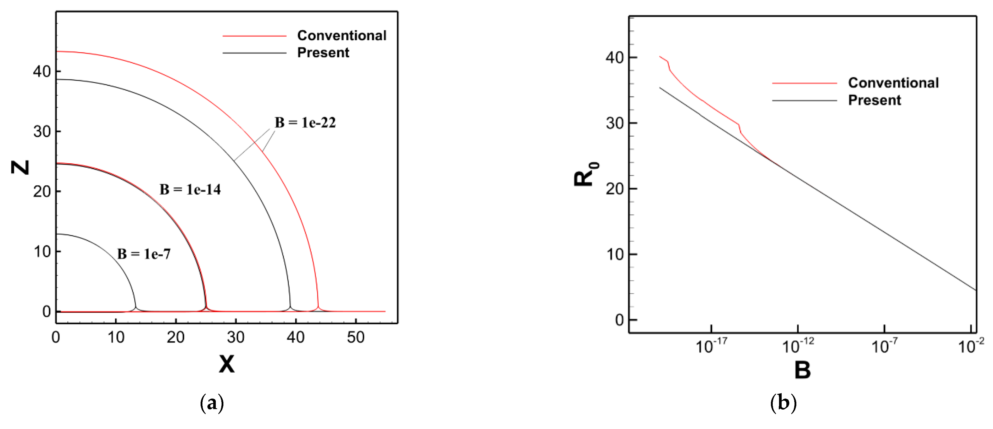
The conventional and improved methods are compared for large bubbles in Figure 5. Here, it can be seen that a smaller value of corresponds to a larger bubble size (Figure 5a). Thus, when 1 × 10⁻⁷, the bubble shapes obtained using the two different methods are almost identical. However, when 1 × 10⁻¹⁴, there is a slight difference between the two results, and when 1 × 10⁻²², the two methods show a significant discrepancy in the obtained bubble shapes. The cause of inaccuracy in the conventional method is demonstrated in Figure 5b, where the dimensionless cap radius is seen to increase abnormally as the parameter decreases in the conventional method.
The conventional and improved methods are compared for small bubbles in Figure 6. Here, when , the bubble shapes obtained using both methods are almost identical (Figure 6a). However, when and , the conventional method raises the bubble in a non-physical manner because the bisection method does not converge and gives a negative value of . As shown in Figure 6b, when is small, the dimensionless absolute height is the same in both methods; however, as becomes larger, fluctuates significantly in the conventional method. These results clearly demonstrate that the improved method should be used to calculate large or small bubbles robustly.
4.2. Comparison of the Present Results with the Earlier Numerical and Experimental Results
The present computational results are compared with the previously published numerical results in Table 1. Various bubble parameters were previously calculated in the range of , , and by Toba [29], Princen [30], and Medrow and Chao [31], respectively. However, Princen [30] used the parameter in place of , where the relationship between these is given by
where denotes the dimensionless parameter of the present work, and denotes the dimensionless parameters of Princen’s work. The computed parameters in Table 1 agree well with one another, with the exception of Toba’s parameters. This is because Toba employed a semi-graphical technique of limited accuracy. The earlier methods used an approximate analytical solution for tiny bubbles [31] or an interpolation method with a pre-calculated Table [30], so the sizes considered were narrow. Medrow and Chao [31] used the boundary conditions of and . Princen [30] searched the junction point until both and were less than . In contrast, the present calculations maintain an accuracy of and , thus providing much more precise results.
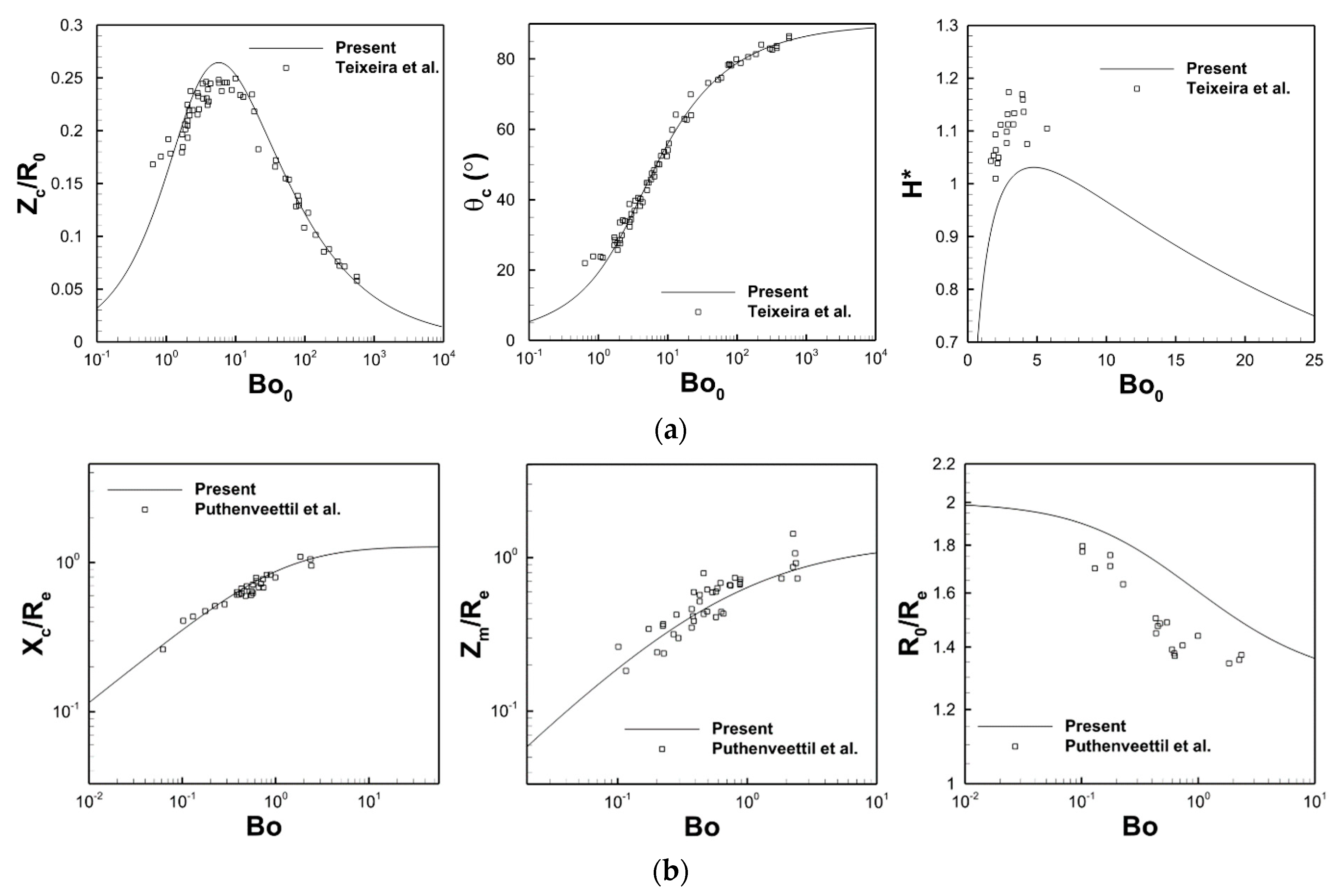
The experimental results of Teixeira et al. [37] are compared with the present numerical results for selected bubble parameters in Figure 7a, where the parameters are plotted with respect to the Bond number based on the cap radius, i.e., . Here, the present computations are seen to agree well with the experimental results, except for the values. For this parameter, the numerical results obtained using Surface Evolver S/W [42] have shown a similar trend to the present computations, as described in [37]. Meanwhile, the experimental results of Puthenveettil et al. [36] are compared with the present numerical results for selected parameters in Figure 7b, where denotes the height of the bubble top above the undisturbed surface. All parameters are normalized with respect to the equivalent bubble radius . The experimental results agree well with the present computation, except that the present computation overestimates the experimental data for . Notably, the numerical results of Puthenveettil et al. [36] also overestimate by a similar amount.
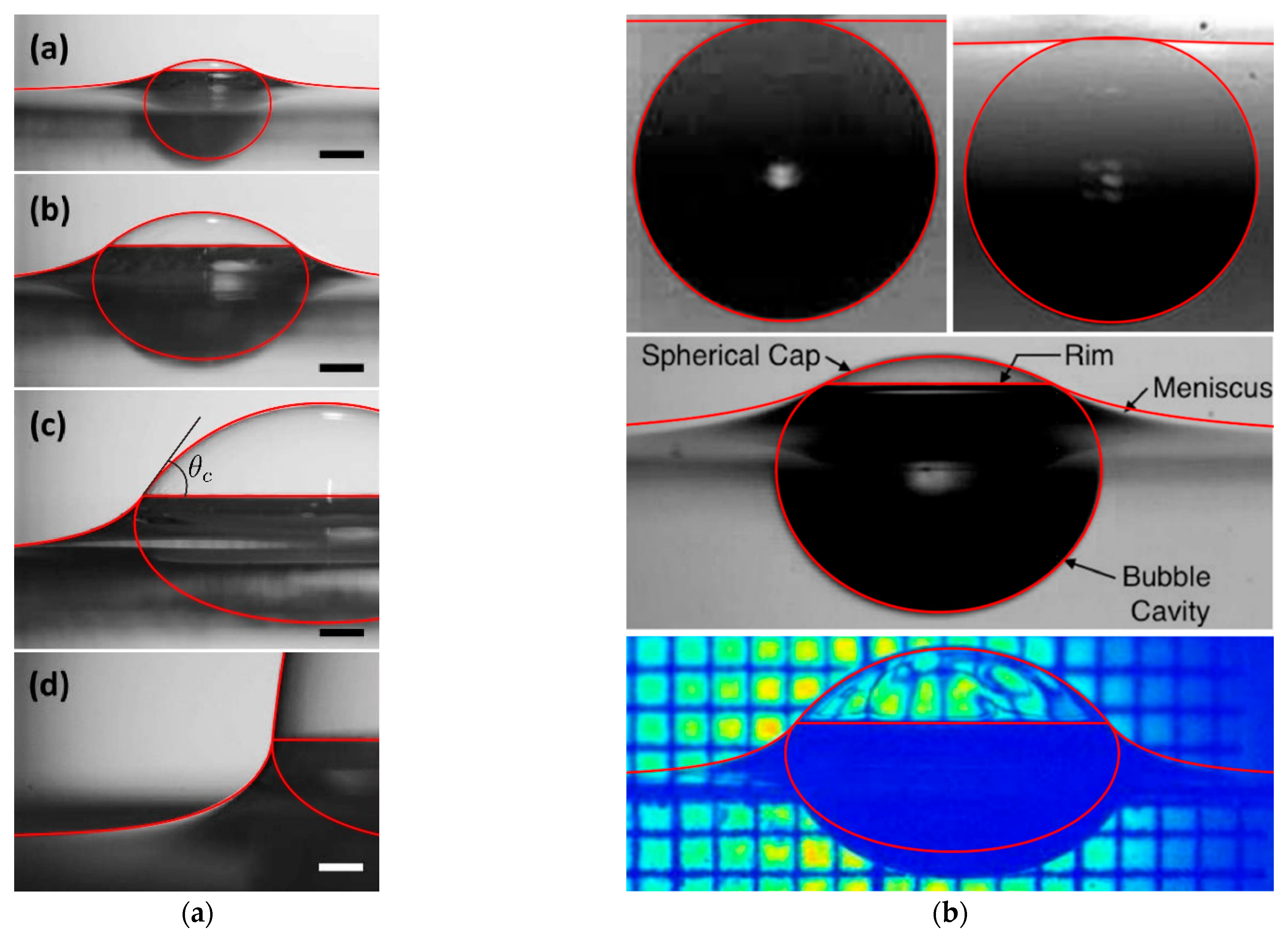
The presently computed profiles for bubbles of various sizes (red outlines) are compared with the experimental photographs obtained by Teixeira et al. [37] and Puthenveettil et al. [36] in Figure 8. In addition, the present predictions for the angle of the junction point ( are compared with those measured by Teixeira et al. [37] in Table 2. Teixeira et al. [37] used a soap solution (), and the images were taken in the range of to (Figure 8a). Here, the calculated bubble shapes are seen to match the experimental images well, although the results in Table 2 indicate slightly different values for the angle of the junction point (). Specifically, the present computational work predicts to be about degrees higher than that measured by Teixeira et al. [37] Meanwhile, the experimental investigations of Puthenveettil et al. [36] were performed on various liquids (e.g., water and ethanol), and the photographs were taken for to (Figure 8b). However, when the Bond numbers measured by Puthenveettil et al. [36] were used in the present computations, the resulting numerical profiles for large bubbles were quite different from the experimental photographs. Hence, the values used in the present work were adjusted in order to provide a better match between the predicted and measured profiles. These adjusted Bond numbers are compared with those measured from Figure 8b in Table 3. Here, similar Bond numbers are predicted and measured for the two tiny bubbles, but the present computations predict much higher Bond numbers than those measured for the two large bubbles. While Teixeira et al. [37] measured the bubble cap radius and the junction angles to obtain an alternative form of Bond number (), Puthenveettil et al. [36] calculated by measuring the volume of a bubble from the experimental image. It is expected that obtaining is more complicated than obtaining because the lower part of the floating bubble is immersed in the liquid, whereas the upper part is not. Therefore, the discrepancy in Table 3 is thought to be due to experimental errors or the limitations of the current theoretical model.
4.3. Important Bubble Parameters and Profiles for a Wide Range of the Bond Numbers
The present numerical results for important bubble parameters in a wide range of Bond numbers (, corresponding to ) are listed in Table 4. The relative tolerance of the ODE solver is set to . For the range of considered here, the present computations satisfy and . Thus, the present method computes the boundary condition of the meniscus more accurately and converges the position of the junction point more precisely than the earlier methods. As a result, the present method provides highly precise and robust numerical results for a wide range of bubble sizes.
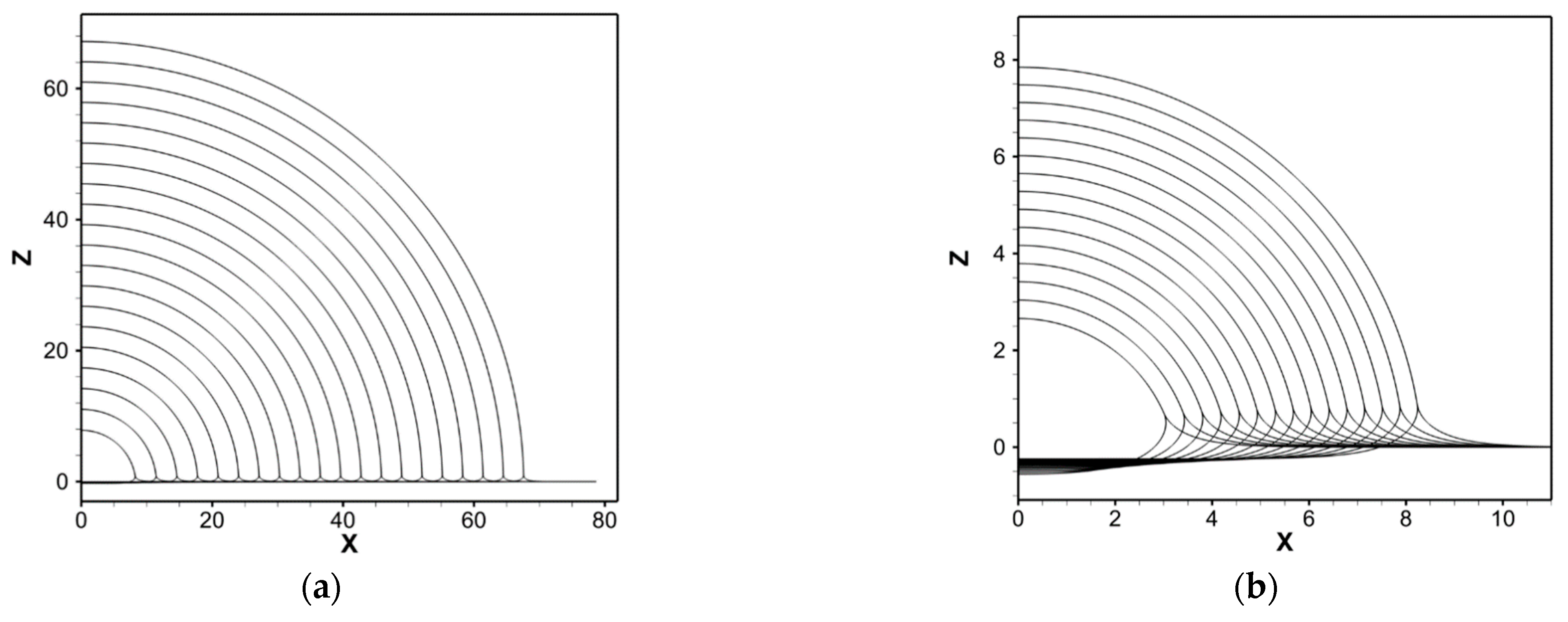
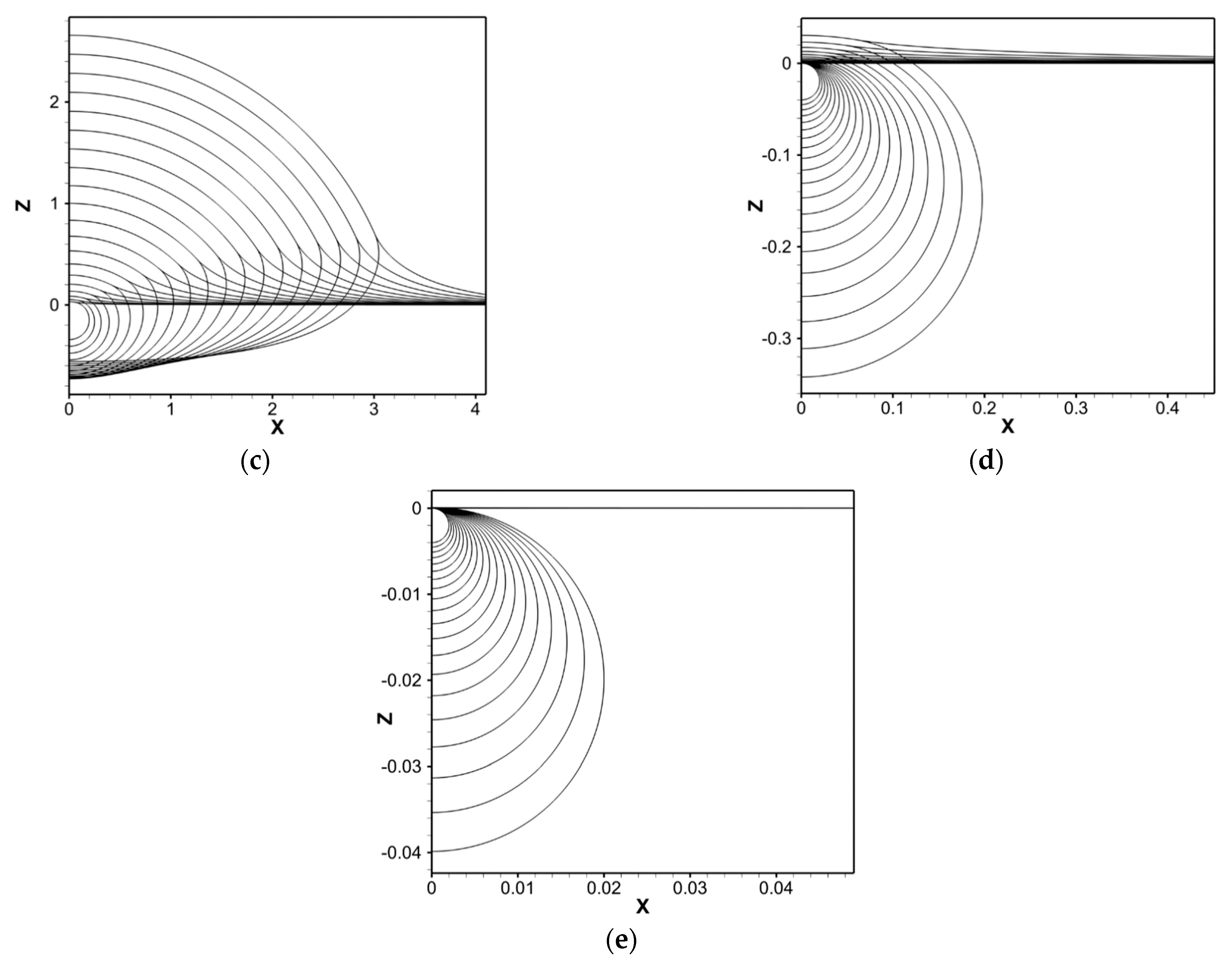
The calculated bubble shapes for are presented in Figure 9, where each shape is drawn at equal intervals on a log scale of . In the interval of to , the bubble exhibits an almost hemispherical shape, and the cavity is virtually flat (Figure 9a). However, in the interval , the shape becomes less hemispherical as the bottom of the bubble continues to descend into the liquid (Figure 9b). In the interval , the shape continues to change from hemispherical to that of a bisected rugby ball (Figure 9c). Interestingly, the depth is found to increase to a maximum value and subsequently decrease within this interval. In the interval , the bubbles have acquired a nearly spherical shape and are seen to protrude only slightly above the undisturbed liquid surface (Figure 9d). Finally, in the interval , the bubbles are almost spherical and are almost entirely submerged in the liquid (Figure 9e).
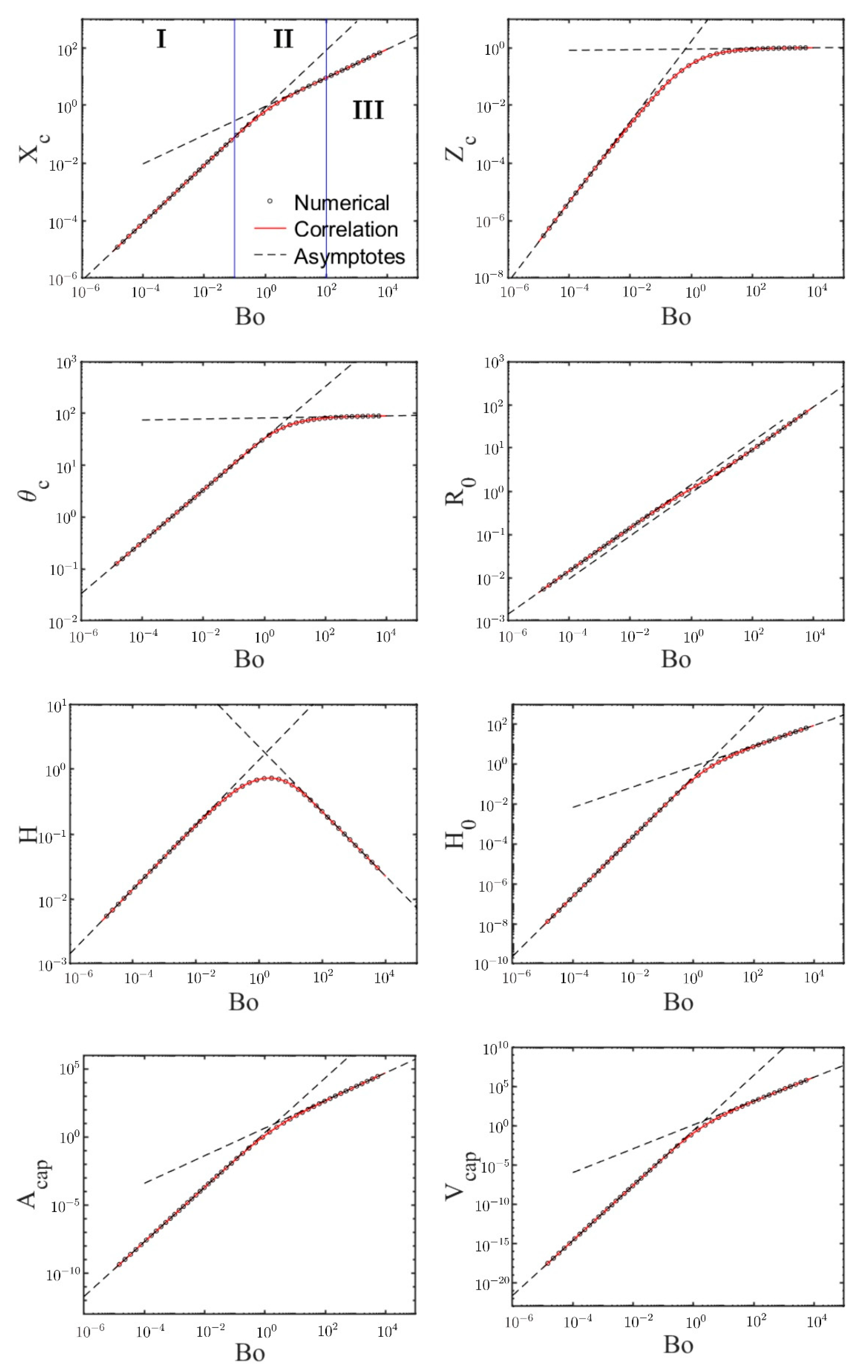
4.4. Correlations and Asymptotic Behaviors of the Bubble Parameters
The log–log plots of the various bubble parameters with respect to the Bond number for the interval of are presented in Figure 10. Each plot can be divided into the following three regions: (I) , (II) , and (III) . The parameters for each interval are fitted with a fifth-order polynomial on the log-log scale according to Equation (28):
where denotes the dimensionless bubble parameters. The coefficients are presented in Table 5.
Interestingly, can be well expressed even with a single “bending function” for , as given by Equation (29):
The curves fitted by the three fifth-order polynomials and by the single bending function are compared in Figure 11, where both correlations are seen to fit the numerical data well.
Two asymptotes appear in Figure 10 as the Bond number goes to zero or infinity. These were obtained numerically via the following simple power law:
where the coefficients and are shown in Table 6.
It is noted that can be rewritten in a more straightforward form as
Furthermore, the asymptotes can be expressed approximately as a power of :
As , , , , , , and .
As , , , , , , , , and .
The height of the undisturbed surface above the bubble bottom has a maximum value of when , as shown in Figure 10.
5. Conclusions
In this study, an improved numerical method was proposed in order to calculate the shape of a floating bubble more precisely and robustly than the conventional method. The proposed method divides the cavity into three parts and accurately finds the location of the connection points at , , , and by defining specific functions and solving them via the root-finding technique. The type of meniscus was used in order to simplify the conventional bisection method, and the improved method was validated by comparison with previously published numerical and experimental results. The bubble shapes and parameters were then obtained precisely for a more extensive range of Bond numbers (), compared to the previously reported range of Bond numbers (. The dimensionless maximum depth of submergence of the bubble below the undisturbed liquid surface was determined as when . The log–log plots of the parameters were divided into three distinct regions of the Bond number, and each interval was fitted with a fifth-order polynomial function. Interestingly, it was possible to fit the parameter with a single correlation for the entire range of Bond numbers. In addition, the asymptotic relations were presented with a simple power law as the Bond number tended to zero or infinity. Moreover, it was possible to approximate most of the bubble parameters to a power of . The correlations and asymptotic equations presented herein are expected to be helpful in scaling models of dynamic bubble-related phenomena such as aerosols and atomization when a bubble bursts.
Funding
This work was supported by the Korea Institute of Energy Technology Evaluation and Planning (KETEP) and the Ministry of Trade, Industry and Energy (MOTIE) of the Republic of Korea (No. 20208901010010).
Institutional Review Board Statement
Not applicable.
Informed Consent Statement
Not applicable.
Data Availability Statement
The data presented in this study are available on request from the corresponding author.
Conflicts of Interest
The author declares no conflict of interest.
Nomenclature
| dimensionless area of the bubble | |
| B | dimensionless pressure difference across the bottom of the bubble |
| Bo | Bond number |
| g | gravitational acceleration, |
| H | dimensionless depth of the bubble below the undisturbed liquid surface |
| p | pressure, |
| equivalent spherical radius of the bubble, | |
| radius of the bubble cap, | |
| , | principal radii of curvature, m |
| dimensionless volume of the bubble | |
| Greek symbols | |
| tangent angle of the meniscus curve | |
| tangent angle of the cavity curve | |
| density, | |
| surface tension, | |
| Subscripts | |
| the junction point | |
| the point where the meniscus meets the undisturbed liquid surface | |
References
- Mason, B.J. The oceans as source of cloud-forming nuclei. Geofis. Pura E Appl. 1957, 36, 148–155. [Google Scholar] [CrossRef]
- Cheng, Y.S.; Zhou, Y.; Irvin, C.M.; Pierce, R.H.; Naar, J.; Backer, L.C.; Baden, D.G. Characterization of marine aerosol for assessment of human exposure to brevetoxins. Environ. Health Perspect. 2005, 113, 638–643. [Google Scholar] [CrossRef] [PubMed] [Green Version]
- Spada, M.; Jorba Casellas, O.; Pérez García-Pando, C.; Janjic, Z.; Baldasano Recio, J.M. Modeling and evaluation of the global sea-salt aerosol distribution: Sensitivity to emission schemes and resolution effects at coastal/orographic sites. Atmos. Chem. Phys. 2013, 13, 11735–11755. [Google Scholar] [CrossRef] [Green Version]
- Dasouqi, A.A.; Yeom, G.S.; Murphy, D.W. Bursting bubbles and the formation of gas jets and vortex rings. Exp. Fluids 2021, 62, 1–18. [Google Scholar] [CrossRef]
- Koch, M.K.; Vossnacke, A.; Starflinger, J.; Schütz, W.; Unger, H. Radionuclide re-entrainment at bubbling water pool surfaces. J. Aerosol. Sci. 2000, 31, 1015–1028. [Google Scholar] [CrossRef]
- Dapper, M.; Wagner, H.J.; Koch, M.K. Assessment of Film Drop Release From Liquid Pools by an Empirical Correlation Approach. Int. Conf. Nucl. Eng. 2008, 48167, 309–314. [Google Scholar]
- Kobayashi, T.; Namiki, A.; Sumita, I. Excitation of airwaves caused by bubble bursting in a cylindrical conduit: Experiments and a model. J. Geophys. Res. Solid Earth 2010, 115, B10. [Google Scholar] [CrossRef] [Green Version]
- Liger-Belair, G.; Cilindre, C.; Gougeon, R.D.; Lucio, M.; Gebefügi, I.; Jeandet, P.; Schmitt-Kopplin, P. Unraveling different chemical fingerprints between a champagne wine and its aerosols. Proc. Natl. Acad. Sci. USA 2009, 106, 16545–16549. [Google Scholar] [CrossRef] [Green Version]
- Illy, E.; Navarini, L. Neglected food bubbles: The espresso coffee foam. Food Biophys. 2011, 6, 335–348. [Google Scholar] [CrossRef] [Green Version]
- Bamforth, C.W. The foaming properties of beer. J. Inst. Brew. 1985, 91, 370–383. [Google Scholar] [CrossRef]
- Hepworth, N.J.; Boyd, J.W.; Hammond, J.R.; Varley, J. Modelling the effect of liquid motion on bubble nucleation during beer dispense. Chem. Eng. Sci. 2003, 58, 4071–4084. [Google Scholar] [CrossRef]
- Mohammed, H.I.; Giddings, D. Multiphase flow and boiling heat transfer modelling of nanofluids in horizontal tubes embedded in a metal foam. Int. J. Therm. Sci. 2019, 146, 106099. [Google Scholar] [CrossRef]
- Mohammed, H.I.; Giddings, D.; Walker, G.S.; Talebizadehsardari, P.; Mahdi, J.M. Thermal behaviour of the flow boiling of a complex nanofluid in a rectangular channel: An experimental and numerical study. Int. Commun. Heat Mass Transf. 2020, 117, 104773. [Google Scholar] [CrossRef]
- Zhang, K.; Li, Y.; Chen, Q.; Lin, P. Numerical study on the rising motion of bubbles near the wall. Appl. Sci. 2021, 11, 10918. [Google Scholar] [CrossRef]
- Nguyen, C.T.; Gonnermann, H.M.; Chen, Y.; Huber, C.; Maiorano, A.A.; Gouldstone, A.; Dufek, J. Film drainage and the lifetime of bubbles. Geochem. Geophys. Geosyst. 2013, 14, 3616–3631. [Google Scholar] [CrossRef] [Green Version]
- Chamkha, A.J.; Doostanidezfuli, A.; Izadpanahi, E.; Ghalambaz, M. Phase-change heat transfer of single/hybrid nanoparticles-enhanced phase-change materials over a heated horizontal cylinder confined in a square cavity. Adv. Powder Technol. 2017, 28, 385–397. [Google Scholar] [CrossRef]
- Ghalambaz, M.; Zadeh, S.M.H.; Mehryan, S.A.M.; Pop, I.; Wen, D. Analysis of melting behavior of PCMs in a cavity subject to a non-uniform magnetic field using a moving grid technique. Appl. Math. Model. 2020, 77, 1936–1953. [Google Scholar] [CrossRef]
- Yeom, G.S.; Chang, K.S. Two-dimensional two-fluid two-phase flow simulation using an approximate Jacobian matrix for HLL scheme. Numer. Heat Transf. Part B Fundam. 2010, 56, 372–392. [Google Scholar] [CrossRef]
- Yeom, G.S.; Chang, K.S. A modified HLLC-type Riemann solver for the compressible six-equation two-fluid model. Comput. Fluids 2013, 76, 86–104. [Google Scholar] [CrossRef]
- Estebe, C.; Liu, Y.; Vahab, M.; Sussman, M.; Moradikazerouni, A.; Shoele, K.; Guo, W. A Low Mach Number, Adaptive Mesh Method for Simulating Multi-phase Flows in Cryogenic Fuel Tanks. In Thermal and Fluids Analysis Workshop (TFAWS); NASA: Washington, DC, USA, 2021. [Google Scholar]
- Hayami, S.; Toba, Y. Drop production by bursting of air bubbles on the sea surface (1) experiments at still sea water surface. J. Oceanogr. Soc. Jpn. 1958, 14, 145–150. [Google Scholar] [CrossRef]
- Boulton-Stone, J.M.; Blake, J.R. Gas bubbles bursting at a free surface. J. Fluid Mech. 1993, 254, 437–466. [Google Scholar] [CrossRef]
- Lhuissier, H.; Villermaux, E. Bursting bubble aerosols. J. Fluid Mech. 2012, 696, 5–44. [Google Scholar] [CrossRef] [Green Version]
- Ghabache, E.; Antkowiak, A.; Josserand, C.; Séon, T. On the physics of fizziness: How bubble bursting controls droplets ejection. Phys. Fluids 2014, 26, 121701. [Google Scholar] [CrossRef] [Green Version]
- Walls, P.L.; Henaux, L.; Bird, J.C. Jet drops from bursting bubbles: How gravity and viscosity couple to inhibit droplet production. Phys. Rev. E 2015, 92, 021002. [Google Scholar] [CrossRef] [PubMed] [Green Version]
- Gañán-Calvo, A.M. Revision of bubble bursting: Universal scaling laws of top jet drop size and speed. Phys. Rev. Lett. 2017, 119, 204502. [Google Scholar] [CrossRef]
- Krishnan, S.; Hopfinger, E.J.; Puthenveettil, B.A. On the scaling of jetting from bubble collapse at a liquid surface. J. Fluid Mech. 2017, 822, 791–812. [Google Scholar] [CrossRef]
- Bashforth, F.; Adams, J.C. An Attempt to Test the Theories of Capillary Action by Comparing the Theoretical and Measured Forms of Drops of Fluid; University Press: Cambridge, UK, 1883. [Google Scholar]
- Toba, Y. Drop production by bursting of air bubbles on the sea surface (II) theoretical study on the shape of floating bubbles. J. Oceanogr. Soc. Jpn. 1959, 15, 121–130. [Google Scholar] [CrossRef] [Green Version]
- Princen, H.M. Shape of a fluid drop at a liquid-liquid interface. J. Colloid Sci. 1963, 18, 178–195. [Google Scholar] [CrossRef]
- Medrow, R.A.; Chao, B.T. Floating bubble configurations. Phys. Fluids 1971, 14, 459–465. [Google Scholar] [CrossRef]
- Bartlett, C.T. Bouncing, Bursting, and Stretching: The Effects of Geometry on the Dynamics of Drops and Bubbles. Ph.D. Dissertation, Boston University, Boston, MA, USA, 2015. [Google Scholar]
- Cohen, C.; Texier, B.D.; Reyssat, E.; Snoeijer, J.H.; Quéré, D.; Clanet, C. On the shape of giant soap bubbles. Proc. Natl. Acad. Sci. USA 2017, 114, 2515–2519. [Google Scholar] [CrossRef] [Green Version]
- Shaw, D.B.; Deike, L. Surface bubble coalescence. J. Fluid Mech. 2021, 915, A105. [Google Scholar] [CrossRef]
- Miguet, J.; Rouyer, F.; Rio, E. The Life of a Surface Bubble. Molecules 2021, 26, 1317. [Google Scholar] [CrossRef] [PubMed]
- Puthenveettil, B.A.; Saha, A.; Krishnan, S.; Hopfinger, E.J. Shape parameters of a floating bubble. Phys. Fluids 2018, 30, 112105. [Google Scholar] [CrossRef]
- Teixeira, M.A.; Arscott, S.; Cox, S.J.; Teixeira, P.I. What is the shape of an air bubble on a liquid surface? Langmuir 2015, 31, 13708–13717. [Google Scholar] [CrossRef] [Green Version]
- Lohnstein, T. Zur Theorie des Abtropfens mit besonderer Rücksicht auf die Bestimmung der Kapillaritätskonstanten durch Tropfversuche. Ann. Phys. 1906, 325, 237–268. [Google Scholar] [CrossRef] [Green Version]
- Yeom, G.S. Comparison of the shapes of isovolumetric bubbles floating on various liquids. J. Comput. Fluids Eng. 2021, 26, 77–83. (In Korean) [Google Scholar] [CrossRef]
- Freud, B.B.; Freud, H.Z. A theory of the ring method for the determination of surface tension. J. Am. Chem. Soc. 1930, 52, 1772–1782. [Google Scholar] [CrossRef]
- Dormand, J.R.; Prince, P.J. A family of embedded Runge-Kutta formulae. J. Comput. Appl. Math. 1980, 6, 19–26. [Google Scholar] [CrossRef] [Green Version]
- Brakke, K.A. The surface evolver. Exp. Math. 1992, 1, 141–165. [Google Scholar] [CrossRef]
Figure 1.
The schematic configuration of a floating bubble.

Figure 2.
Comparison of the bubble shapes obtained according to the boundary point of Equations (8) and (9) for a large bubble (B = ) using (a) the conventional method, and (b) the improved method involving the root-finding technique. The tolerance of the ODE solver is set to . The insets plot the cavity profiles up to 45 degrees and are not scaled.

Figure 3.
Comparison of the bubble shapes obtained according to the tolerance of the ODE solver for a large bubble (B = ) using (a) the conventional method, and (b) the improved method involving the root-finding technique. The insets plot the cavity profiles up to 45 degrees and are not scaled.
Figure 3.
Comparison of the bubble shapes obtained according to the tolerance of the ODE solver for a large bubble (B = ) using (a) the conventional method, and (b) the improved method involving the root-finding technique. The insets plot the cavity profiles up to 45 degrees and are not scaled.

Figure 4.
Three types of the meniscus shape according to the location of the guessed junction point. Here, is the angle at the exact junction point.
Figure 4.
Three types of the meniscus shape according to the location of the guessed junction point. Here, is the angle at the exact junction point.

Figure 5.
Comparison of the conventional (red) and the improved (black) methods for large bubbles. The tolerance of the ODE solver is set to . (a) Floating bubble shapes for the following three large bubble sizes: = 1 × 10⁻⁷, 1 × 10⁻¹⁴, and 1 × 10⁻²². (b) The dimensionless cap radius is plotted with respect to the parameter .

Figure 6.
Comparison of the conventional (red) and the improved (black) methods for small bubbles. The tolerance of the ODE solver is set to . (a) Floating bubble shapes for the following three small bubble sizes: = 1000, 2000, and 3000. (b) The dimensionless absolute height is plotted with respect to the parameter .

Figure 7.
Comparison of the present numerical results with the experimental results of (a) Teixeira et al. [37] and (b) Puthenveettil et al. [36] for selected bubble parameters, where .

Figure 8.
Comparison of the presently computed bubble profiles (red outlines) with the experimental photographs obtained by (a) Reprinted with permission from [37]. Copyright 2015 American Chemical Society (from top to bottom = (a) 1, (b) 2.1, (c) 4.2 and (d) 32.5 mm) and (b) Reprinted from [36], with the permission of AIP Publishing.

Figure 9.
The computed bubble shapes for , where each shape is drawn at equal intervals on a log scale of . (a) Twenty bubbles for (. (b) Fifteen bubbles for (. (c) Twenty bubbles for (. (d) Twenty bubbles for (. (e) Twenty bubbles for (.
Figure 9.
The computed bubble shapes for , where each shape is drawn at equal intervals on a log scale of . (a) Twenty bubbles for (. (b) Fifteen bubbles for (. (c) Twenty bubbles for (. (d) Twenty bubbles for (. (e) Twenty bubbles for (.


Figure 10.
Correlation and two asymptotes of the computed bubble parameters as a function of the Bond number on a log–log scale. The correlation is given by a fifth-order polynomial function in each of the three Bond number regions (I, II, and III). The two asymptotes are given by a power law.
Figure 10.
Correlation and two asymptotes of the computed bubble parameters as a function of the Bond number on a log–log scale. The correlation is given by a fifth-order polynomial function in each of the three Bond number regions (I, II, and III). The two asymptotes are given by a power law.

Figure 11.
Comparison of the fitting results of the fifth-order polynomials and bending function for .
Figure 11.
Comparison of the fitting results of the fifth-order polynomials and bending function for .


Table 1.
Comparison of the present numerical results with those of Toba [29], Princen [30], and Medrow and Chao [31] for the selected bubble parameters.
| Authors | |||||||
|---|---|---|---|---|---|---|---|
| 50 | Medrow | 0.0026045 | 0.07970 | 178.13 | 0.07975 | 0.0002672 | 0.07921 |
| Present | 0.002604455 | 0.07958193 | 178.1285 | 0.07974769 | 0.000267229 | 0.07909536 | |
| 20 | Toba | 0.016 | 0.194 | 175.3 | 0.196 | 0.0041 | 0.184 |
| Medrow | 0.016011 | 0.19481 | 175.32 | 0.1963 | 0.004108 | 0.1897 | |
| Present | 0.01601056 | 0.1947944 | 175.3211 | 0.1962769 | 0.004107305 | 0.1896872 | |
| 8 | Princen | 0.09101 | 0.44341 | 168.443 | 0.45428 | 0.05846 | - |
| Present | 0.09100837 | 0.4434090 | 168.4433 | 0.4542754 | 0.05846040 | 0.4026157 | |
| 7 | Toba | 0.117 | 0.493 | 166.5 | 0.502 | 0.0863 | 0.433 |
| Medrow | 0.11520 | 0.49307 | 166.88 | 0.5076 | 0.08463 | 0.4401 | |
| Present | 0.1152068 | 0.4930890 | 166.8816 | 0.5075995 | 0.08463203 | 0.4401145 | |
| 4 | Toba | 0.284 | 0.722 | 158.4 | 0.772 | 0.3680 | 0.592 |
| Princen | 0.28217 | 0.72309 | 158.574 | 0.77245 | 0.36408 | - | |
| Medrow | 0.28217 | 0.72310 | 158.57 | 0.7724 | 0.3641 | 0.5892 | |
| Present | 0.2821735 | 0.7230909 | 158.5740 | 0.7724442 | 0.3640805 | 0.5891839 | |
| 2 | Toba | 0.655 | 0.989 | 145.9 | 1.169 | 1.67 | 0.711 |
| Princen | 0.65599 | 0.98789 | 146.014 | 1.17354 | 1.67520 | - | |
| Medrow | 0.65598 | 0.98782 | 146.02 | 1.174 | 1.675 | 0.7042 | |
| Present | 0.6559949 | 0.9878898 | 146.0140 | 1.173535 | 1.675189 | 0.7042526 | |
| 1 | Toba | 1.159 | 1.161 | 134.2 | 1.621 | 5.51 | 0.734 |
| Medrow | 1.1603 | 1.15854 | 134.56 | 1.629 | 5.505 | 0.7281 | |
| Present | 1.160338 | 1.158526 | 134.5617 | 1.628556 | 5.505488 | 0.7280821 | |
| 0.5 | Princen | 1.71400 | 1.23904 | 125.860 | 2.11488 | 13.7728 | - |
| Medrow | 1.7140 | 1.23890 | 125.87 | 2.115 | 13.77 | 0.6956 | |
| Present | 1.714005 | 1.239067 | 125.8599 | 2.114874 | 13.77346 | 0.6956826 | |
| 0.4 | Princen | 1.89485 | 1.25155 | 123.611 | 2.27520 | 17.6919 | - |
| Medrow | 1.8948 | 1.25152 | 123.61 | 2.275 | 17.69 | 0.6790 | |
| Present | 1.894856 | 1.251574 | 123.6100 | 2.275215 | 17.69363 | 0.6790378 | |
| 0.001 | Medrow | 6.5244 | 1.14954 | 101.91 | 6.668 | 565.2 | 0.2994 |
| Present | 6.524375 | 1.149610 | 101.9076 | 6.667858 | 565.2013 | 0.2994464 | |
| 4 × 10⁻⁸ | Medrow | 13.947 | 1.07121 | 95.66 | 14.02 | 5527 | 0.1427 |
| Present | 13.94652 | 1.071357 | 95.6803 | 14.01534 | 5523.744 | 0.1427007 |
Table 2.
The angle of the junction point ( ) as measured experimentally by Teixeira et al. [37] and as predicted in the present work.
Table 2.
The angle of the junction point ( ) as measured experimentally by Teixeira et al. [37] and as predicted in the present work.
| Image in Figure 8a | ||
|---|---|---|
| Teixeira et al. [37] | Present | |
| (a) | 25.7 | 26.6 |
| (b) | 38.5 | 39.6 |
| (c) | 52.5 | 54.7 |
| (d) | 83.9 | 84.2 |
Table 3.
The Bond numbers (BO) measured by Puthenveettil et al. [36] and those of the present computational work.
Table 3.
The Bond numbers (BO) measured by Puthenveettil et al. [36] and those of the present computational work.
| Image in Figure 8b | ||
|---|---|---|
| Puthenveettil et al. [36] | Present | |
| Top Left | 0.004 | 0.004 |
| Top Right | 0.03 | 0.03 |
| Middle | 0.5 | 0.63 |
| Bottom | 2.46 | 3.5 |
Table 4.
The present numerical results for important bubble parameters.
| Bo | H | ||||||
|---|---|---|---|---|---|---|---|
| 1000 | 7.999957 × 10⁻⁶ | 6.531920 × 10⁻⁶ | 1.426955 × 10⁻⁷ | 179.9064 | 0.003999773 | 5.333294 × 10⁻⁹ | 0.003999968 |
| 500 | 3.199932 × 10⁻⁵ | 2.612705 × 10⁻⁵ | 8.835825 × 10⁻⁷ | 179.8129 | 0.007998500 | 4.266541 × 10⁻⁸ | 0.007999744 |
| 300 | 8.888362 × 10⁻⁵ | 7.257102 × 10⁻⁵ | 3.674190 × 10⁻⁶ | 179.6881 | 0.01332701 | 1.975148 × 10⁻⁷ | 0.01333215 |
| 200 | 0.0001999733 | 0.0001632667 | 1.131729 × 10⁻⁵ | 179.5322 | 0.01998027 | 6.665443 × 10⁻⁷ | 0.01999600 |
| 150 | 0.0003554713 | 0.0002902067 | 2.500423 × 10⁻⁵ | 179.3762 | 0.02662265 | 1.579731 × 10⁻⁶ | 0.02665720 |
| 100 | 0.0007995738 | 0.0006526751 | 7.571394 × 10⁻⁵ | 179.0643 | 0.03986447 | 5.329410 × 10⁻⁶ | 0.03996813 |
| 80 | 0.001248960 | 0.001019346 | 0.0001385365 | 178.8304 | 0.04974934 | 1.040468 × 10⁻⁵ | 0.04993789 |
| 60 | 0.002218939 | 0.001810413 | 0.0002997670 | 178.4404 | 0.06611566 | 2.464071 × 10⁻⁵ | 0.06652007 |
| 30 | 0.008836790 | 0.007193843 | 0.001842383 | 176.8804 | 0.1297692 | 0.0001958917 | 0.1321897 |
| 20 | 0.01973977 | 0.01601056 | 0.005107188 | 175.3211 | 0.1896872 | 0.0006540912 | 0.1962769 |
| 16 | 0.03062309 | 0.02474611 | 0.008773140 | 174.1542 | 0.2317490 | 0.001263504 | 0.2429617 |
| 10 | 0.07610977 | 0.06055737 | 0.02561974 | 170.6915 | 0.3420357 | 0.004930032 | 0.3743891 |
| 7 | 0.1483636 | 0.1152068 | 0.05297453 | 166.8816 | 0.4401145 | 0.01324675 | 0.5075995 |
| 4 | 0.3924363 | 0.2821735 | 0.1339070 | 158.5740 | 0.5891839 | 0.05338361 | 0.7724442 |
| 2 | 1.085626 | 0.6559949 | 0.2836372 | 146.0140 | 0.7042526 | 0.2004702 | 1.173535 |
| 1 | 2.399762 | 1.160338 | 0.4304443 | 134.5617 | 0.7280821 | 0.4858354 | 1.628556 |
| 0.5 | 4.422484 | 1.714005 | 0.5433848 | 125.8599 | 0.6956826 | 0.8759713 | 2.114874 |
| 0.2 | 8.186136 | 2.454823 | 0.6454278 | 117.9642 | 0.6195963 | 1.476051 | 2.779336 |
| 0.1 | 11.82990 | 3.007428 | 0.6984155 | 113.8375 | 0.5582908 | 1.959115 | 3.287901 |
| 0.03 | 19.73677 | 3.948336 | 0.7613356 | 108.9106 | 0.4642022 | 2.820973 | 4.173604 |
| 0.002 | 44.66426 | 6.005879 | 0.8378743 | 102.8796 | 0.3236288 | 4.787607 | 6.160882 |
| 2 × 10⁻⁵ | 109.3486 | 9.416629 | 0.8949651 | 98.35707 | 0.2101250 | 8.134374 | 9.517693 |
| 4 × 10⁻⁸ | 240.5064 | 13.94652 | 0.9286565 | 95.68030 | 0.1427007 | 12.62814 | 14.01534 |
| 3 × 10⁻¹² | 537.2599 | 20.80127 | 0.9520342 | 93.82031 | 0.09593434 | 19.45857 | 20.84759 |
| 2 × 10⁻¹⁸ | 1197.575 | 30.99599 | 0.9677704 | 92.56740 | 0.06445970 | 29.63729 | 31.02714 |
| 1 × 10⁻²⁵ | 2310.565 | 42.99781 | 0.9767552 | 91.85180 | 0.04648970 | 41.63011 | 43.02028 |
| 1 × 10−40 | 5723.091 | 67.57905 | 0.9852057 | 91.17865 | 0.02958871 | 66.20297 | 67.59335 |
| B | V | A | |||||
| 1000 | 0.001999997 | 2.592758 × 10⁻⁵ | 3.351005 × 10⁻⁸ | 5.026523 × 10⁻⁵ | 0.6035815 | −1.525375 × 10⁻²² | 2.676590 × 10⁻⁸ |
| 500 | 0.003999979 | 9.281963 × 10⁻⁵ | 2.680740 × 10⁻⁷ | 0.0002010577 | 1.730274 | −7.698510 × 10⁻²² | 1.453944 × 10⁻⁸ |
| 300 | 0.006666568 | 0.0002463152 | 1.241013 × 10⁻⁶ | 0.0005584724 | 2.985969 | −3.153570 × 10⁻²² | 7.827400 × 10⁻⁹ |
| 200 | 0.009999667 | 0.0005332463 | 4.187953 × 10⁻⁶ | 0.001256470 | 3.535465 | −1.123335 × 10⁻²¹ | 1.095687 × 10⁻⁸ |
| 150 | 0.01333254 | 0.0009204409 | 9.925456 × 10⁻⁶ | 0.002233493 | 5.149609 | −2.827164 × 10⁻²² | 2.132361 × 10⁻⁹ |
| 100 | 0.01999733 | 0.001979302 | 3.348354 × 10⁻⁵ | 0.005023872 | 6.959408 | −2.696805 × 10⁻²³ | 4.713860 × 10⁻¹⁰ |
| 80 | 0.02499480 | 0.003009708 | 6.536818 × 10⁻⁵ | 0.007847453 | 6.050189 | −3.036618 × 10⁻²² | 3.593450 × 10⁻⁹ |
| 60 | 0.03332100 | 0.005150905 | 0.0001547967 | 0.01394203 | 6.122253 | −3.366391 × 10⁻²² | 7.635189 × 10⁻⁹ |
| 30 | 0.06656836 | 0.01842589 | 0.001230227 | 0.05552427 | 7.955407 | −1.988549 × 10⁻²² | 3.939505 × 10⁻⁹ |
| 20 | 0.09967012 | 0.03801315 | 0.004107305 | 0.1240385 | 8.408457 | −4.855708 × 10⁻²³ | 6.727939 × 10⁻⁹ |
| 16 | 0.1243594 | 0.05600981 | 0.007936283 | 0.1924426 | 9.236173 | −1.191350 × 10⁻²¹ | 3.836083 × 10⁻⁹ |
| 10 | 0.1974393 | 0.1218416 | 0.03109598 | 0.4785621 | 9.861832 | −3.807630 × 10⁻²² | 5.996772 × 10⁻⁹ |
| 7 | 0.2785360 | 0.2086884 | 0.08463203 | 0.9340670 | 10.87842 | −2.663932 × 10⁻²² | 3.687912 × 10⁻⁹ |
| 4 | 0.4664155 | 0.4271852 | 0.3640805 | 2.483857 | 11.63113 | −6.332112 × 10⁻²³ | 5.348933 × 10⁻⁹ |
| 2 | 0.8182227 | 0.8158624 | 1.675189 | 6.968744 | 12.57281 | −8.638849 × 10⁻²² | 6.609880 × 10⁻⁹ |
| 1 | 1.278940 | 1.265220 | 5.505488 | 15.69547 | 12.89420 | −3.031094 × 10⁻²¹ | 1.564443 × 10⁻⁸ |
| 0.5 | 1.796671 | 1.728766 | 13.77346 | 29.45927 | 13.99436 | −1.192995 × 10⁻²¹ | 9.942357 × 10⁻⁹ |
| 0.2 | 2.507679 | 2.341705 | 34.68663 | 55.64825 | 14.57138 | −6.057025 × 10⁻²¹ | 1.638346 × 10⁻⁸ |
| 0.1 | 3.046686 | 2.803791 | 60.25804 | 81.40699 | 15.50268 | −9.881551 × 10⁻²² | 1.074786 × 10⁻⁸ |
| 0.03 | 3.973631 | 3.606096 | 129.8547 | 138.0179 | 17.51656 | −8.436210 × 10⁻²² | 2.649258 × 10⁻⁹ |
| 0.002 | 6.017921 | 5.421926 | 442.0626 | 319.0965 | 18.42952 | −1.661529 × 10⁻²¹ | 1.674617 × 10⁻⁸ |
| 2 × 10⁻⁵ | 9.421791 | 8.550337 | 1693.416 | 794.3151 | 21.75908 | −7.942353 × 10⁻²¹ | 2.212266 × 10⁻⁸ |
| 4 × 10⁻⁸ | 13.94893 | 12.82268 | 5523.744 | 1764.149 | 25.96071 | −2.333522 × 10⁻²⁰ | 3.959115 × 10⁻⁸ |
| 3 × 10⁻¹² | 20.80236 | 19.40908 | 18,442.52 | 3967.061 | 33.13493 | −5.203562 × 10⁻²¹ | 2.737275 × 10⁻⁸ |
| 2 × 10⁻¹⁸ | 30.99649 | 29.33207 | 61,375.84 | 8881.418 | 43.50420 | −2.452283 × 10⁻²⁰ | 2.283753 × 10⁻⁸ |
| 1 × 10⁻²⁵ | 42.99807 | 41.10880 | 164,482.9 | 17,177.59 | 54.76092 | −8.969384 × 10⁻²⁰ | 6.884084 × 10⁻⁸ |
| 1 × 10−40 | 67.57916 | 65.37684 | 641,194.2 | 42644.47 | 80.35356 | −1.015233 × 10⁻²⁰ | 1.705349 × 10⁻⁸ |
Table 5.
Coefficients of the fifth-order polynomial for fitting the bubble parameters.
| Parameter | Interval | ||||||
|---|---|---|---|---|---|---|---|
| 5 × 10⁻⁵ < Bo < 0.1 | −0.1735 | 0.8713 | −0.07803 | −0.02357 | −0.003523 | −0.0002078 | |
| 0.1 < Bo < 100 | −0.2107 | 0.7763 | −0.1426 | −0.001089 | 0.02162 | −0.004812 | |
| 100 < Bo < 5000 | −0.1349 | 0.6468 | −0.09254 | 0.02825 | −0.004265 | 0.0002566 | |
| 5 × 10⁻⁵ < Bo < 0.1 | −0.5639 | 0.6232 | −0.3526 | −0.09327 | −0.01357 | −0.000821 | |
| 0.1 < Bo < 100 | −0.5699 | 0.6353 | −0.2707 | 0.01518 | 0.02576 | −0.006322 | |
| 100 < Bo < 5000 | −0.5019 | 0.5271 | −0.2434 | 0.06047 | −0.007931 | 0.0004324 | |
| 5 × 10⁻⁵ < Bo < 0.1 | 1.561 | 0.5498 | 0.02396 | 0.005715 | 0.0006714 | 0.00003092 | |
| 0.1 < Bo < 100 | 1.517 | 0.4145 | −0.1141 | −0.02333 | 0.01714 | −0.002079 | |
| 100 < Bo < 5000 | 1.529 | 0.4392 | −0.1993 | 0.04873 | −0.006298 | 0.0003392 | |
| 5 × 10⁻⁵ < Bo < 0.1 | 0.03884 | 0.3443 | −0.08807 | −0.02505 | −0.003558 | −0.000201 | |
| 0.1 < Bo < 100 | 0.05469 | 0.4101 | 0.00479 | 0.01815 | −0.00413 | −0.0004402 | |
| 100 < Bo < 5000 | 0.04825 | 0.3953 | 0.04915 | −0.01243 | 0.001658 | −0.0000919 | |
| H | 5 × 10⁻⁵ < Bo < 0.1 | −0.1509 | 0.1079 | −0.2103 | −0.05746 | −0.007922 | −0.0004377 |
| 0.1 < Bo < 100 | −0.1561 | 0.1188 | −0.1691 | −0.03095 | −0.0007063 | 0.006116 | |
| 100 < Bo < 5000 | 0.2356 | −0.3661 | −0.0688 | 0.01897 | −0.002739 | 0.0001626 | |
| 5 × 10⁻⁵ < Bo < 0.1 | −0.6643 | 1.432 | −0.0471 | −0.01573 | −0.002533 | −0.000158 | |
| 0.1 < Bo < 100 | −0.7411 | 1.215 | −0.2392 | −0.02608 | 0.03433 | −0.005775 | |
| 100 < Bo < 5000 | −0.6902 | 1.182 | −0.319 | 0.07998 | −0.01055 | 0.0005778 | |
| 5 × 10⁻⁵ < Bo < 0.1 | 0.1727 | 1.777 | −0.1352 | −0.04078 | −0.006091 | −0.000359 | |
| 0.1 < Bo < 100 | 0.1118 | 1.626 | −0.2344 | −0.007935 | 0.0302 | −0.006215 | |
| 100 < Bo < 5000 | 0.1562 | 1.578 | −0.2698 | 0.06755 | −0.008896 | 0.0004859 | |
| 5 × 10⁻⁵ < Bo < 0.1 | −0.8076 | 3.187 | −0.1962 | −0.06074 | −0.009259 | −0.0005546 | |
| 0.1 < Bo < 100 | −0.9542 | 2.794 | −0.5047 | −0.02876 | 0.07281 | −0.01439 | |
| 100 < Bo < 5000 | −0.7944 | 2.578 | −0.525 | 0.1361 | −0.01844 | 0.001031 |
Table 6.
Coefficients of the power law for asymptotic relations.
| Parameter | Limit | ||
|---|---|---|---|
| 0.8163 | 1 | ||
| 0.9063 | 0.4983 | ||
| 1.646 | 1.395 | ||
| 0.8945 | 0.01123 | ||
| 33.09 | 0.5 | ||
| 81.56 | 0.009909 | ||
| 1.414 | 0.5 | ||
| 0.9104 | 0.4978 | ||
| H | 1.409 | 0.4997 | |
| 2.197 | −0.4978 | ||
| 0.2357 | 1.5 | ||
| 0.7787 | 0.5136 | ||
| 2.094 | 2 | ||
| 4.454 | 1.011 | ||
| 0.2467 | 3.5 | ||
| 1.246 | 1.517 |
Publisher’s Note: MDPI stays neutral with regard to jurisdictional claims in published maps and institutional affiliations. |
© 2022 by the author. Licensee MDPI, Basel, Switzerland. This article is an open access article distributed under the terms and conditions of the Creative Commons Attribution (CC BY) license (https://creativecommons.org/licenses/by/4.0/).
Share and Cite
MDPI and ACS Style
Yeom, G.-S. Correlations and Asymptotic Behaviors of the Shape Parameters of Floating Bubbles Using an Improved Numerical Procedure. Appl. Sci. 2022, 12, 1804. https://doi.org/10.3390/app12041804
AMA Style
Yeom G-S. Correlations and Asymptotic Behaviors of the Shape Parameters of Floating Bubbles Using an Improved Numerical Procedure. Applied Sciences. 2022; 12(4):1804. https://doi.org/10.3390/app12041804
Chicago/Turabian StyleYeom, Geum-Su. 2022. "Correlations and Asymptotic Behaviors of the Shape Parameters of Floating Bubbles Using an Improved Numerical Procedure" Applied Sciences 12, no. 4: 1804. https://doi.org/10.3390/app12041804
Note that from the first issue of 2016, this journal uses article numbers instead of page numbers. See further details here.