
Extreme Learning Machine Using Bat Optimization Algorithm for Estimating State of Health of Lithium-Ion Batteries


1
School of Mechanical Engineering, University of Shanghai for Science and Technology, Shanghai 200093, China
2
Institute of Transportation, Zhejiang Industry Polytechnic College, Shaoxing 312000, China
3
School of Vehicle and Mobility, Tsinghua University, Beijing 100084, China
*
Authors to whom correspondence should be addressed.
Appl. Sci. 2022, 12(3), 1398; https://doi.org/10.3390/app12031398
Submission received: 28 December 2021
/
Revised: 22 January 2022
/
Accepted: 25 January 2022
/
Published: 28 January 2022
(This article belongs to the Special Issue Intelligent Renewable Energy System: A Focus on Hydrogen Fuel Cells and Battery Storage with AI)
Abstract
:An accurate estimation of the state of health (SOH) of lithium-ion batteries is essential for the safe and reliable operation of electric vehicles. As a single hidden-layer feedforward neural network, extreme learning machine (ELM) has the advantages of a fast learning speed and good generalization performance. The bat algorithm (BA) is a swarm intelligence optimization algorithm based on bat echolocation for foraging. In this study, BA was creatively applied to improve the ELM neural network, forming a BA-ELM model, and it was applied to SOH estimation for the first time. First, through Pearson and Spearman correlation analysis, six variables were determined as the input variables of the model. The actual remaining capacity of the battery was determined as the output variable. Second, BA was used to optimize the connection weights and bias in ELM to construct the BA-ELM model. Third, the battery data set was trained and tested with BA-ELM, ELM, Elman, back propagation (BP), radial basis function (RBF), and general regression neural network (GRNN) models. Five statistical error indicators, and the radar chart, scatter plot, and violin diagram were used to compare the estimation effects. The results show that the evaluation function of BA-ELM can converge quickly and effectively optimize the network model of ELM. The RMSE of the BA-ELM model was 0.5354%, and the MAE was 0.4326%, which is the smallest among the 6 models. The RMSE values of the other model were 2.27%, 3.53%, 3.07%, 3.86%, 3.24%, respectively, indicating the BA-ELM has good potential for future applications.
1. Introduction
Because of global warming, environmental pollution, energy shortages, and many other challenges, electric vehicles are becoming increasingly more popular as a green, efficient, and sustainable ideal transportation tool [1]. Lithium-ion batteries have become an ideal power source for electric vehicles because of their high energy density, long cycle life, and low self-discharge rate [2]. The batteries will age with repeated use, which will decrease the battery’s charge and discharge capacity and the actual remaining capacity [3,4]. State of health (SOH) is a quantitative indicator used for evaluating the degree of battery aging. Generally, SOH is defined as the ratio of the actual remaining capacity of the battery to the rated capacity of the battery [5]. The accuracy estimation of the battery state of charge (SOC) and the cruising range of the electric vehicle both depend on the accurate estimation of the battery SOH [6]. In addition, aging batteries are more prone to thermal runaway [7]. Therefore, it is very important to evaluate reliable methods and strategies to accurately estimate the current remaining capacity and SOH of the battery.
At present, SOH estimation methods mainly include direct measurement-based estimation, model-based estimation, and data-based estimation. The direct measurement-based method estimates the battery SOH by measuring the battery’s characteristic parameters, such as the voltage, current, temperature, and internal resistance. Weng et al. [8] proposed a method to measure the available battery capacity based on the mapping relationship between SOC and open-circuit voltage (OCV). However, as the battery ages or the ambient temperature changes, the SOC and OCV curves must be corrected again. Galeotti et al. [9] proposed a method for the performance analysis of lithium-ion batteries and SOH estimation through electrochemical impedance spectroscopy (EIS). Although the EIS method can accurately characterize the battery status, this method can generally only be performed in a laboratory or under relatively stable conditions [10]. This also limits the use of this method in real vehicles or in online situations. Significant efforts have been made to study the model-based method to estimate the SOH and capacity of batteries. A method combining the Kalman filter and equivalent circuit model (ECM) was developed to estimate the SOH of lithium-ion batteries [11,12]. Mastali and Li et al. proposed electrochemical models to describe the lithium-ion diffusion and migration inside a battery [13,14]. This type of model needs to input a lot of physical and chemical parameters, leading to the need to solve a series of algebraic equations and partial differential equations. How to balance the complexity and computational efficiency of this method is worthy of further study. With the development of artificial intelligence and the Internet, the data-based method has received increasingly more attention. This method is based on battery laboratory measurements or actual operating data of electric vehicles to achieve SOH estimation through algorithms, such as neural networks [15]. Kristen et al. [16] applied machine-learning tools to both predict and classify cells by their cycle life with the discharge–voltage curves obtained from the early cycles to determine capacity degradation. The result showed a 4.9% test error when the first 5 cycles were used for classifying the cycle life. Support vector machine (SVM) is a widely used machine learning technique [17,18,19]. Tian et al. reported a deep convolutional neural network for capacity estimation based on measurements during charging [20]. Based on the BP neural network, a three-layer BP neural network was trained to estimate the SOH at a low computational cost [21]. Li et al. [22] proposed a variant long-short-term memory (LSTM) neural network. An NASA dataset was trained for the prediction of SOH and remaining service life, and the RMSE of the result was low.
Among the many machine learning methods, ELM has the advantages of a simple structure and easy adjustment of parameters [23]. Compared with the SVM and BP neural network models, ELM has a faster training speed, it does not easily fall into local optimality, and its generalization ability is better [24,25]. Based on a stacked denoising autoencoders ELM algorithm, Li et al. [26] proposed a big data-driven battery modeling method (SDAE-ELM). The battery data extracted from electric buses were used to validate the effectiveness and accuracy of the model. Wang et al. [27] proposed a novel robust ELM model to improve the estimation capability. The mean square error (MSE) in ELM was substituted by a mixture-generalized maximum correntropy criterion. This method solved the non-Gaussian complex noise interference problem to a certain extent. Chen et al. [28] proposed a novel metabolic extreme learning machine (M-ELM) framework to describe the complex battery degradation mechanism that can reflect the latest degradation trend. Ma et al. [29] developed a new broad learning-ELM (BL-ELM). The feature and enhancement nodes were merged to become the new input layer of the network. This can provide the benefit of reducing the calculation time. Mariani et al. [30] proposed a modified biogeography-based approach to optimize ELM for pressure prediction of a spark ignition single-cylinder engine. The type of activation function, number of hidden layer nodes, and sparse connection structure were obtained using the new approach. A possible improvement in ELM design lies in attribute selection instead of using all variables in the predictive model. Adnan et al. [31] proposed a new hybrid ELM model combined with grey wolf optimization (WO) and hybrid particle swarm optimization (PSO) for streamflow prediction. The new model reduced the RMSE in prediction effectively. However, it was found that the PSOGWO algorithm is not very stable compared with the PSO and PSOGSA algorithms. Bardhan et al. [32] proposed a novel hybrid of the ELM and adaptive neuro swarm intelligence techniques for the determination of the California bearing ratio of soils. The results of the hybrid model were better than other ELM-based models. To fully utilize the advantages of different algorithms, the development of a hybrid method for ELM and other optimization algorithms has become a new research direction.
On the other hand, BA is a swarm intelligence optimization algorithm based on bat echolocation for hunting [33]. As a metaheuristic algorithm used for searching for the global optimal solution, the BA provides a completely different solution to the optimization problem [34,35]. Yang et al. [36] proposed an enhanced adaptive BA for optimal energy scheduling in a microgrid system. Because of the different search mechanisms applied in the early and late search stages, the search performance improved. Shivaie et al. [37] developed a reliability-constrained cost-effective model to identify the optimal sizing of an autonomous hybrid renewable system. The bat search algorithm was used to obtain the final optimal solution. Based on a hybrid bat algorithm (BA)-harmony search algorithm technique, Peddakapu et al. [38] proposed a new two-degree freedom-tilted integral derivative with a filter controller for a two-area wind-hydro-diesel power system. A sensitivity analysis showed that the robustness of the controller was improved. Thus, the BA has global exploration and local exploitation capabilities, and it is entirely possible to use it to optimize the ELM model.
Based on the above discussion, the main contributions of this study are as follows:
- A globally optimized BA can be used to optimize the connection weights and bias of the ELM neural network. The BA-ELM model can be creatively constructed.
- The relevant data of the battery can be analyzed by Pearson and Spearman correlation; thus, the data can be determined scientifically and reasonably.
- Through a convergence analysis of the BA algorithm, the optimization effect can be further evaluated.
- Through a comparison of BA-ELM, ELM, BP, Elman, RBF, and GRNN, the effectiveness of the proposed model and the performance of SOH estimation can be comprehensively evaluated.
The structure of this paper is arranged as follows: Section 2 provides an overview of the standard ELM and BA algorithms. Section 3 describes the data acquisition and processing related to the battery charge and discharge test. Section 4 provides detailed information about the BA-ELM model. Section 5 reports a comparison with another 5 neural network models. Section 6 provides conclusions and future work directions.
2. Methods for SOH Estimation
2.1. ELM
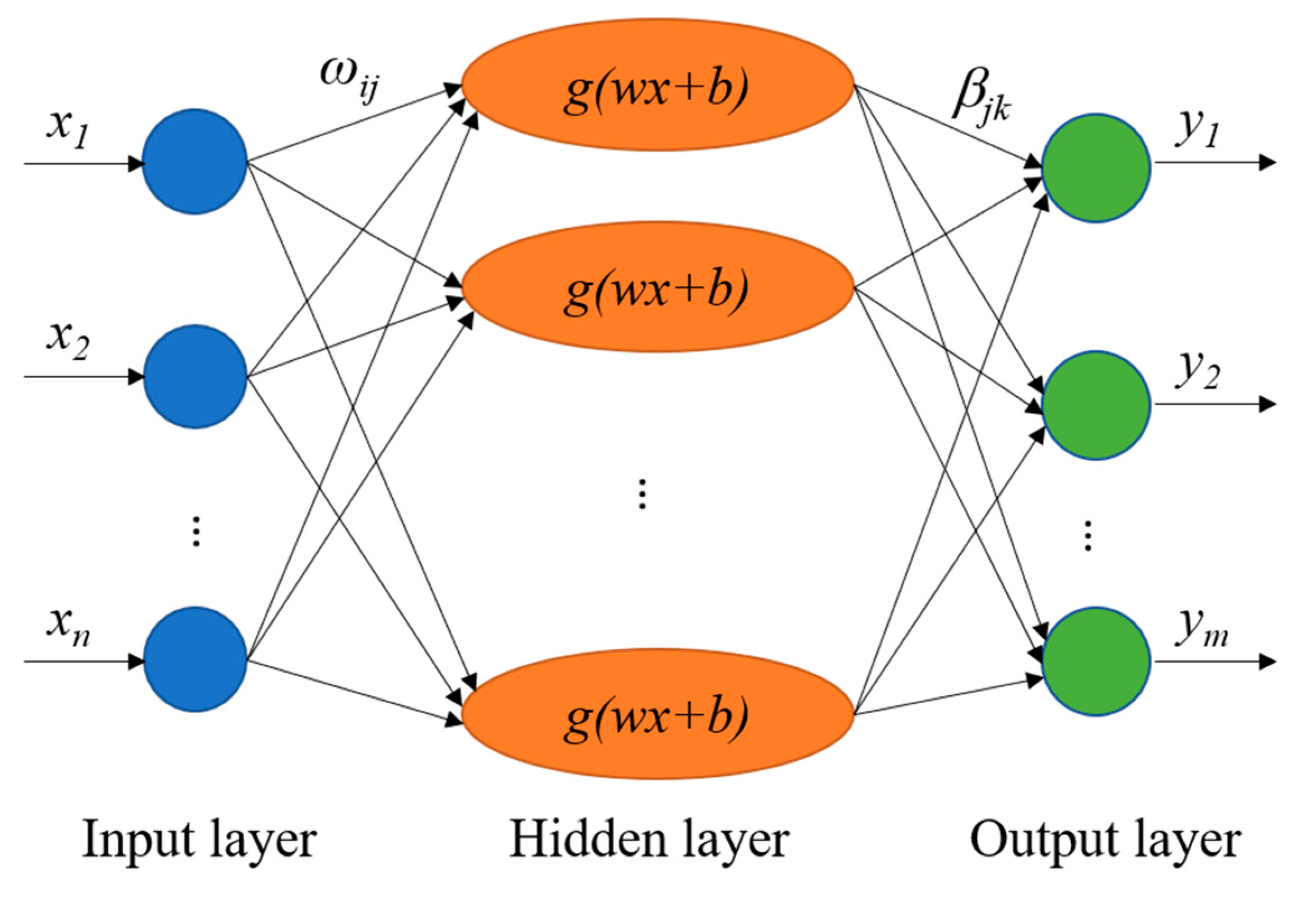
Huang et al. [39] first proposed relevant theories and applications of ELM in 2006. The structure of the classic ELM model is mainly composed of an input layer, a hidden layer, and an output layer, as shown in Figure 1. The input layer has n neurons, i.e., n input variables x. The output layer has m neurons, i.e., m output variables y. The hidden layer has l neurons. ωij represents the connection weight between the i-th neuron in the input layer and the j-th neuron in the hidden layer. βjk represents the connection weight between the j-th neuron in the hidden layer and the k-th neuron in the output layer. g(⋅) is the activation function, b is the bias of the hidden layer, X is the input matrix, Y is the output matrix, and the number of training samples is Q. The main steps of the ELM algorithm are shown in Table 1.

Table 1.
Algorithmic process of ELM.
| Algorithm of ELM |
|---|
| Step 1: The number of neurons in the input layer n, hidden layer l, and output layer m are determined separately. The connection weight ω between the hidden layer and the input layer and the bias b of the hidden layer are randomly set. |
| Step 2: The activation function of the hidden layer neurons g(x) is determined, then the hidden layer output matrix H is calculated. |
| Step 3: The connection weight β between the output layer and the hidden layer is calculated by the formula β = H+YT. |
The output Y of the ELM neural network can be calculated using Equation (4):
where H is the hidden layer output matrix of the ELM neural network, as shown in Equation (5):
The connection weight β between the output layer and hidden layer can be calculated using the least squares solution of Equation (6):
The solution can be expressed as follows:
The estimation of SOH based on the neural network algorithm is a new artificial intelligence method. As a single hidden-layer feedforward neural network, ELM has the advantages of a fast learning speed, high calculation efficiency, and good generalization performance. However, during the establishment of ELM, the number of hidden layer neurons is not fixed, and the connection weight and threshold are randomly set, which may cause the battery SOH estimation to be inaccurate. To overcome these shortcomings, we tried to use the BA optimization algorithm to improve the SOH estimation performance of ELM.
2.2. BA
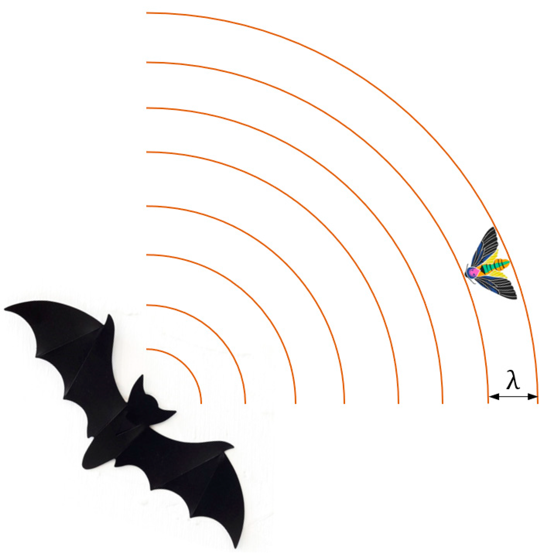
Bats emit ultrasonic waves through their mouths. When the ultrasonic waves encounter prey or obstacles, they reflect back to form an echo, which is received by the bat’s ears. The bat relies on these echoes for accurate positioning, which allows it to fly freely and hunt accurately in a completely dark environment, as shown in Figure 2. Interestingly, the wavelength of the ultrasonic waves emitted by bats is very close to the size of the prey. Inspired by this fact, Yang first proposed the theory and basic framework of the BA in 2010 [40]. BA is a heuristic algorithm used for searching for the global optimal solution. The main steps of BA are shown in Table 2, where x∗ is the current global optimal solution.
The flight frequency of the bat can be obtained using Equation (9), where rand ∈ [0, 1] is a random vector obtained from a uniform distribution. According to the sound wave calculation formula, the speed is the multiplication of the wavelength and the frequency. Thus, the flying speed of the bat can be obtained using Equation (10). The position of the bat can be obtained using Equation (11). fmin represents the bat with the smallest fitness; BestS is the position corresponding to the bat with the smallest fitness, i.e., the current best position, where α and γ are constants; A is the loudness; and r is the pulse emission rate:
The BA changes the frequency randomly, providing a good global exploration and optimization ability. The local exploitation capabilities are enhanced by varying the loudness and pulse emission rate. The BA uses tuning technology to control the dynamic behavior of the bat population. The fitness function is used to compare the pros and cons of each bat’s location. Survival of the fittest in a bat colony is likened to an iterative process of replacing poorer feasible solutions with good feasible solutions. The characteristics of the BA provide a completely different solution to the optimization problem. Therefore, we tried to use the BA algorithm to optimize the connection weights and bias in the ELM model.
3. Data Acquisition and Processing
3.1. Data Acquisition
In this study, the battery data set obtained from the NASA Prognostic Center of Excellence (PCoE) was used for related research [41]. The B6 lithium-ion battery of NASA has a rated capacity of 2 Ah. The battery was charged and discharged at room temperature, and the data, such as the voltage, current, and battery temperature, were collected. First, the battery was charged in the 1.5 A constant current mode until the battery voltage reached 4.2 V. Then, the battery was continuously charged in a constant voltage mode until the charging current dropped to 20 mA. Next, the battery was discharged in the 2A constant current mode until the voltage dropped to 2.5 V. As the battery was repeatedly charged and discharged, the available capacity of the battery decayed. The experiment was stopped when the actual battery capacity dropped from 2 to 1.2 Ah.
We further sorted out the data of the eight variables in the experiment, namely, the constant current charging time TI, constant voltage charging time TV, total charging time Ttotal,charge, battery voltage change at charging ΔVcharge, total discharge time Ttotal,discharge, battery temperature change during discharge ΔTempdischarge, battery voltage change at discharge ΔVdischarge, and the actual remaining capacity of battery Caged. The relationship between the actual remaining capacity and number of cycles is shown in Figure 3.
3.2. Data Processing
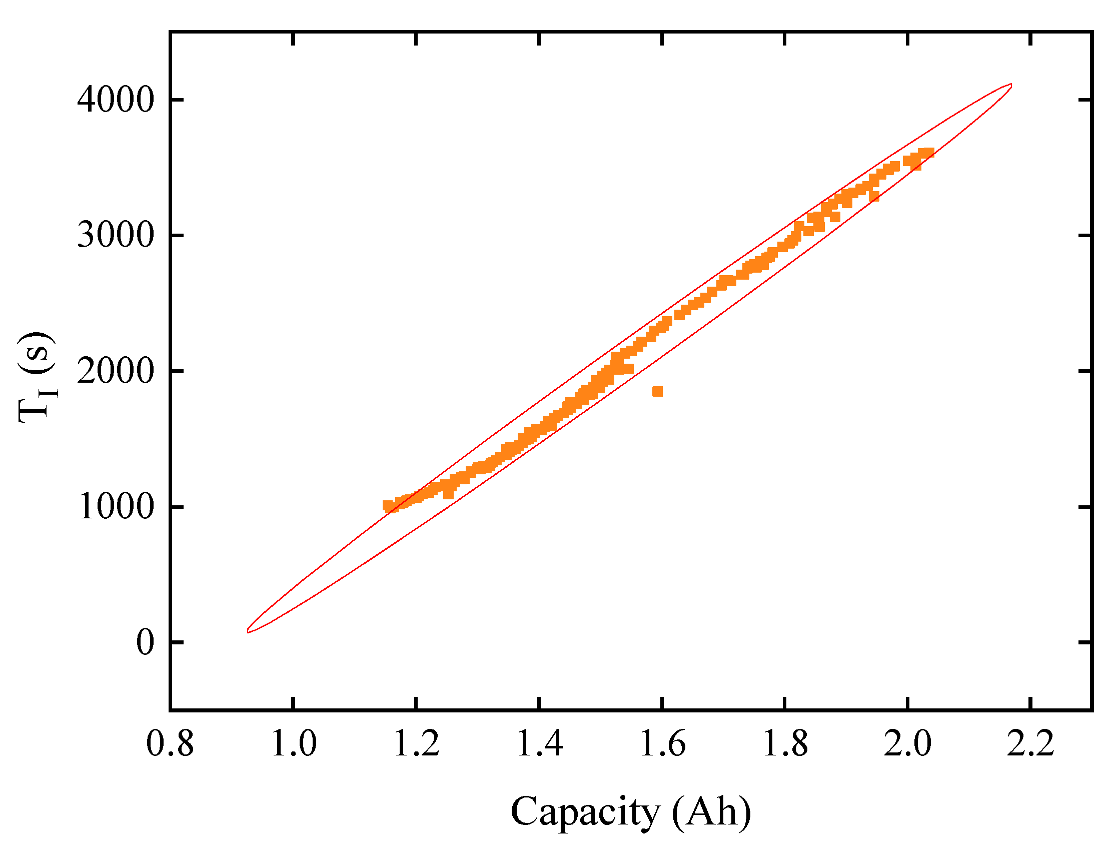
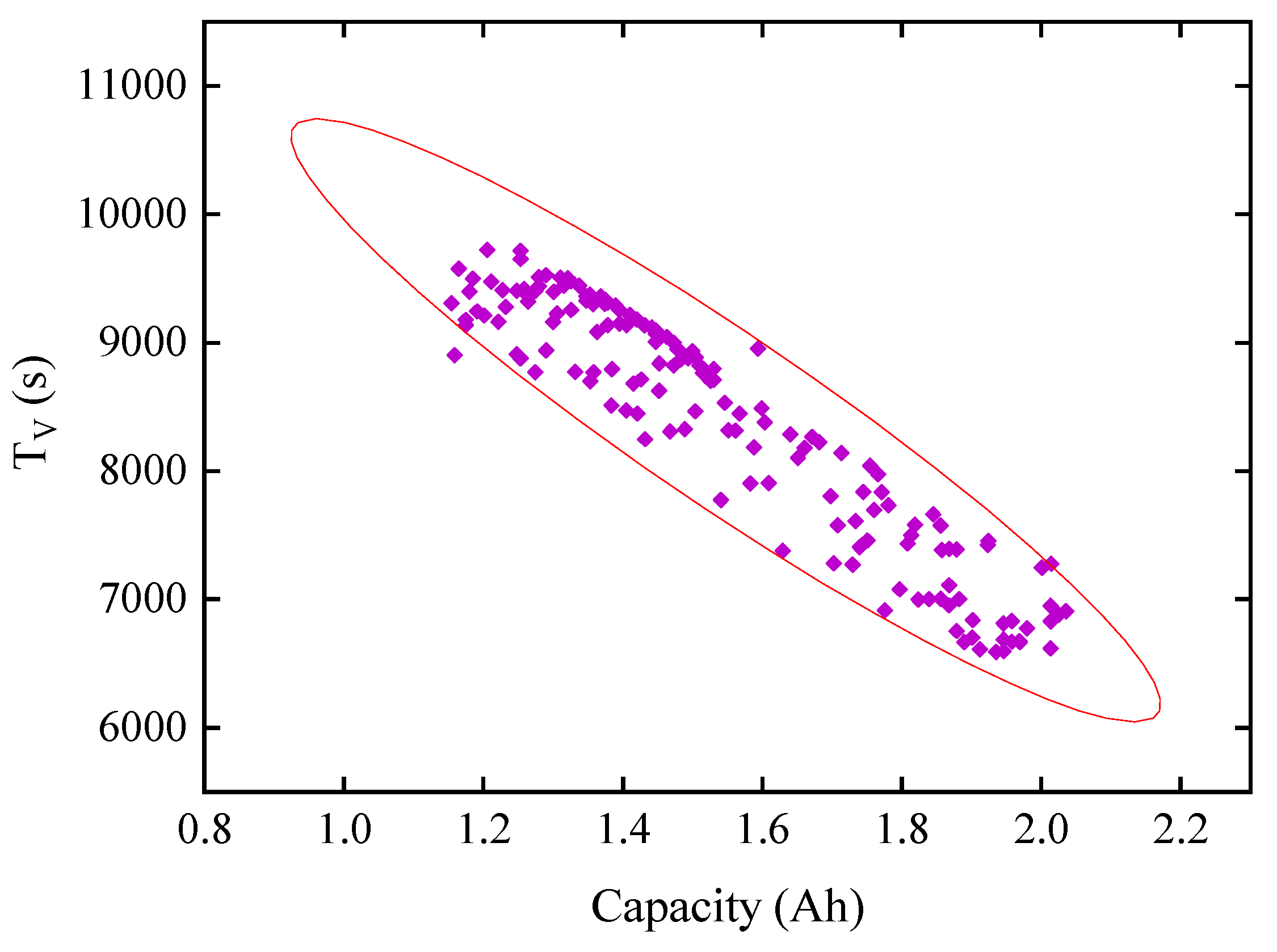
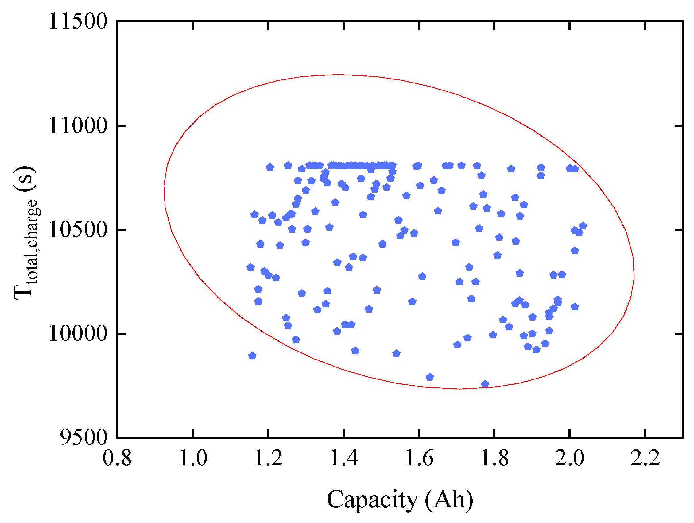
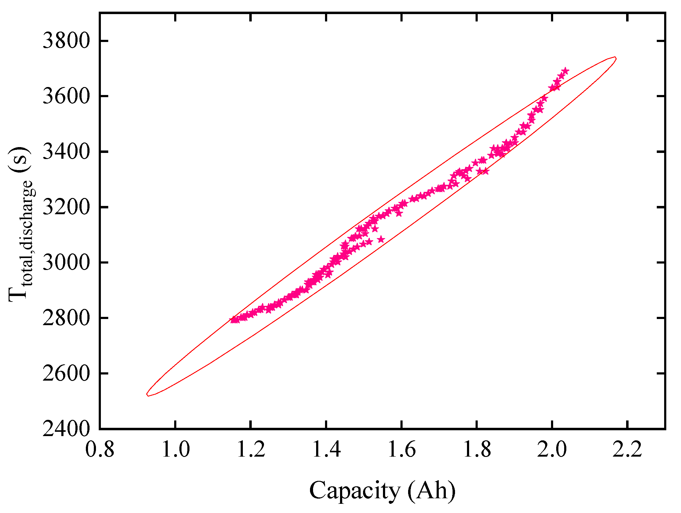
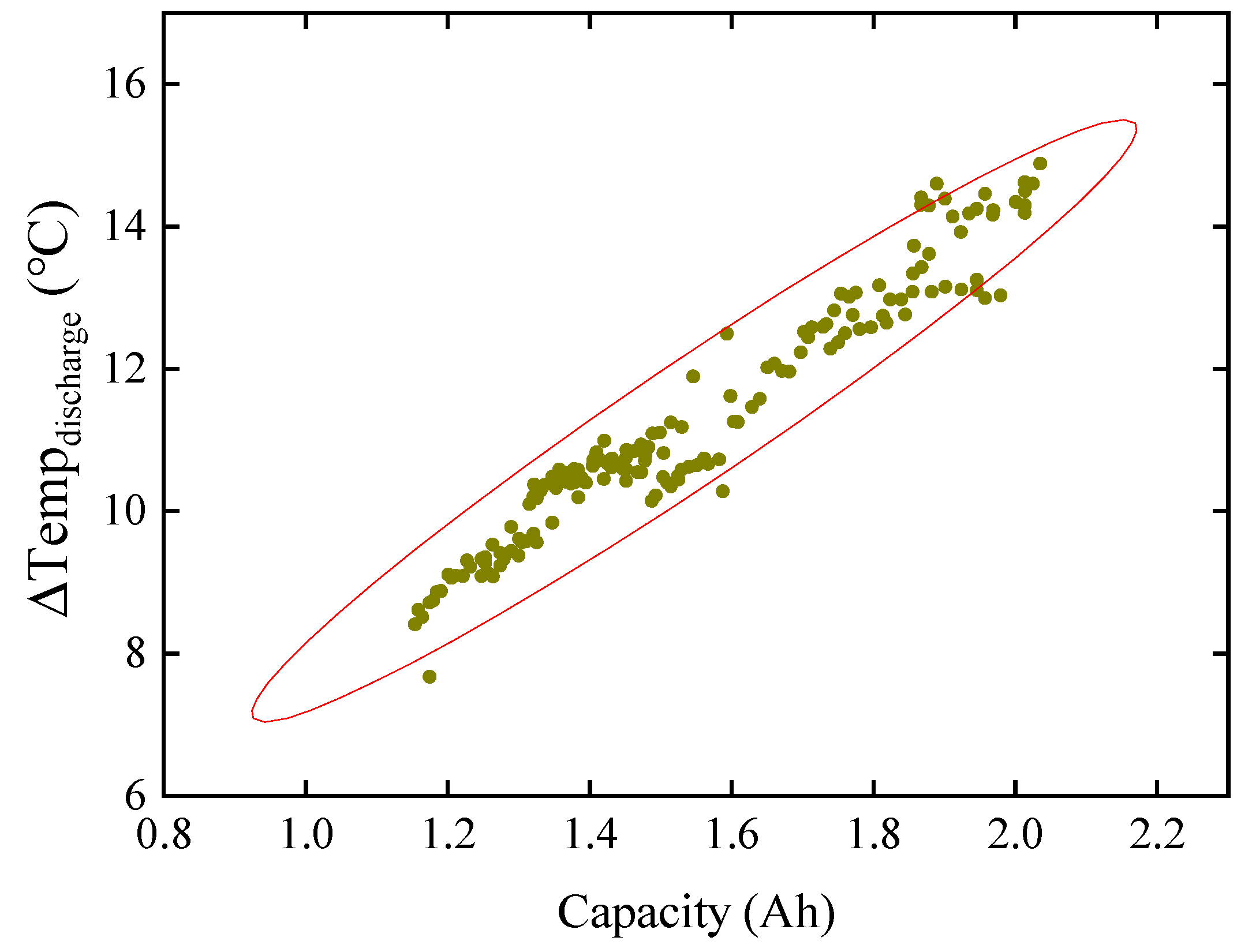
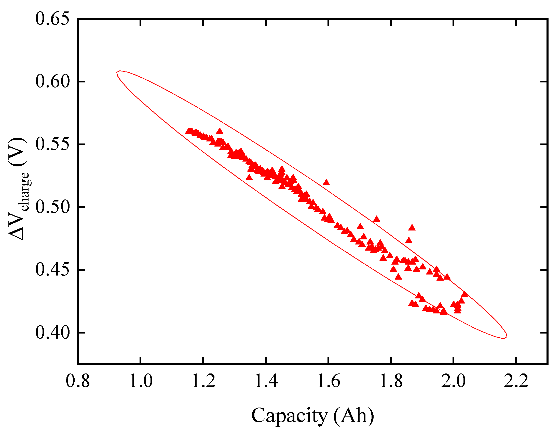
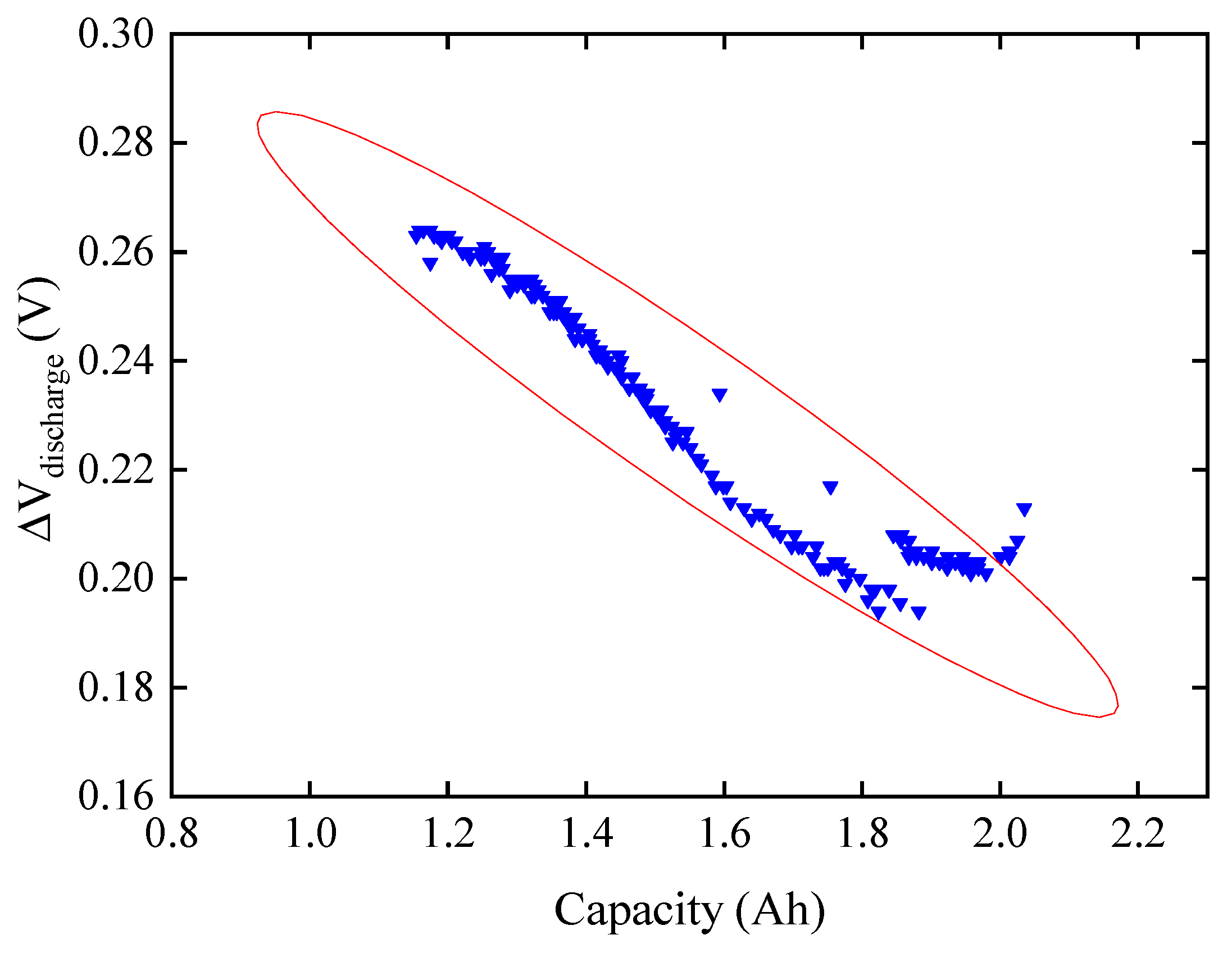
To determine the input data of the neural network more scientifically and reasonably, we first drew the scatter figures between the 7 variables of the battery and the actual remaining capacity, and added a confidence ellipse to the scatter figure, where the confidence level of the ellipse was 95%, as shown in Figure 4, Figure 5, Figure 6, Figure 7, Figure 8, Figure 9 and Figure 10. Then, the eight variables of the battery were analyzed for the Pearson and Spearman correlation analyses. The coefficient of Pearson assesses the linear correlation between two variables while the coefficient of Spearman assesses the monotonic relationship between two variables. Taking the two variables of X and Y as examples, the coefficient of Pearson could be obtained using Equation (14), and the coefficient of Spearman could be obtained using Equation (15), where di is the difference of the rank of the i-th data pair, and N is the number of samples. Table 3 shows the judgment criteria between the degree of correlation and the correlation coefficient. The results are shown in Table 4.
Analyzing Figure 4, Figure 5, Figure 6, Figure 7, Figure 8, Figure 9 and Figure 10 and Table 4, the coefficients of Spearman corresponding to TI, Ttotal,discharge, and ΔTempdischarge are all positive. This shows that the relationship between these three variables and the available remaining capacity monotonically increased. The coefficients of Spearman corresponding to TV, Ttotal,charge, ΔVcharge, and ΔVdischarge are all negative, indicating that the relationship between these four variables and the available remaining capacity monotonically decreased. In Figure 4, the ratio of the long axis to the short axis of the confidence ellipse corresponding to TI is the largest, and the coefficients of Pearson and Spearman are the largest. This indicates that the linear correlation between TI and the actual remaining capacity is the largest, and the monotonic correlation is the strongest. The absolute value of the Pearson and Spearman coefficients of Ttotal,charge is the smallest, and the ratio of the major axis to the minor axis of the confidence ellipse corresponding to Ttotal,charge is the smallest, indicating that the correlation between Ttotal,charge and the actual remaining capacity is the smallest.
According to the absolute value of Pearson’s correlation coefficient, the order of linear correlation can be expressed as follows:
TI > Ttotal,discharge > ΔVcharge > ΔTempdischarge > ΔVdischarge > TV > Ttotal,charge
According to the absolute value of Spearman’s correlation coefficient, the order of monotonic correlation is as follows:
TI > Ttotal,discharge > ΔVcharge > ΔVdischarge > ΔTempdischarge > TV > Ttotal,charge
Through a comparative analysis, the variable Ttotal,charge with the lowest correlation was eliminated. The constant current charging time TI, constant voltage charging time TV, battery voltage change at charging ΔVcharge, total discharge time Ttotal,discharge, battery temperature change during discharge ΔTempdischarge, and battery voltage change at discharge ΔVdischarge were determined as the input variables of the model. The actual remaining capacity of the battery Caged was determined as the output variable.
In this study, the values of the six input variables have different dimensional ranges. For example, the min value of ΔVdischarge is 0.2; the max value of TV is 9800; the difference between the two is 49,000 times. The large gap will oscillate the neural network model back and forth when the gradient is updated, and affect the final accuracy of the model. Therefore, Equation (16) was used to uniformly process the values of the 6 input variables and converted them into an interval of [−1, 1], where ymin and ymax are the minimum and maximum values of y. In all the samples, 70% of the data were randomly selected for training, and the remaining 30% for testing:
4. The Proposed Model
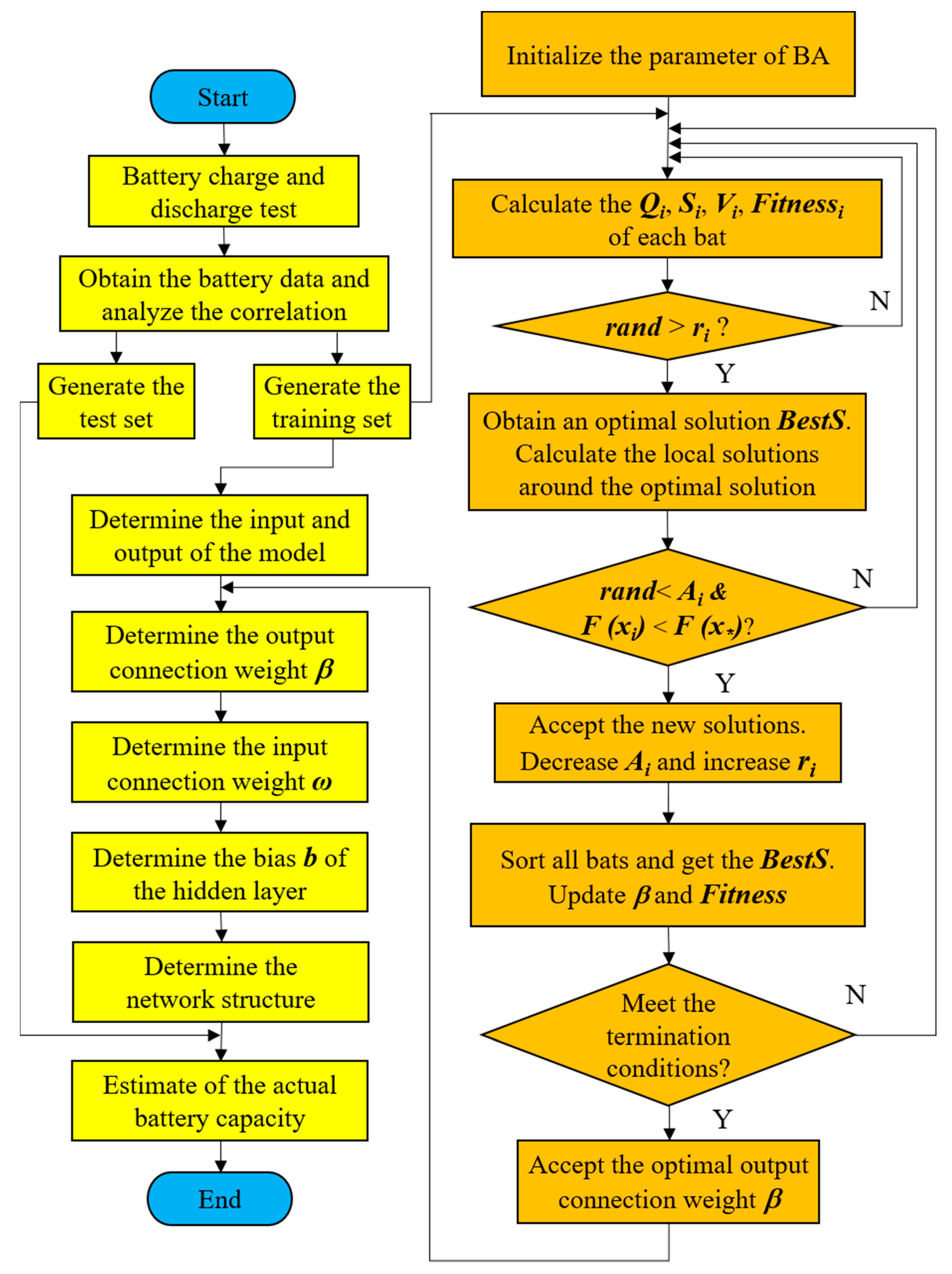
In this study, we proposed a BA-ELM model and applied it to estimate battery SOH for the first time. The process of SOH estimation based on the BA-ELM model is shown in Figure 11. The pseudo code of BA-ELM is shown in Table 5. The main steps are as follows:
S1: Battery charge and discharge test.
The lithium-ion battery was charged and discharged at room temperature. The specific test process is described in Section 3.1.
S2: Obtain the battery data and analyze the correlation.
- (1).
- The data of the eight variables in the test were sorted. The sample data were normalized to the same dimension range: 70% of the data were randomly selected for training, and the remaining 30% was tested.
- (2).
- Through Pearson and Spearman correlation analysis, TI, TV, Ttotal,discharge, ΔVcharge, ΔTempdischarge, and ΔVdischarge were determined as the input variables of the model, and Caged was determined as the output variable.
S3: The global exploring ability of the BA was used to optimize the output connection weight, input connection weight, and bias b of the hidden layer of the ELM.
- (1).
- Initialize the parameter of BA.
- (2).
- While t < the max number of iterations; calculate the frequency Qi, location Si, speed Vi, and fitness of each bat.
- (3).
- If rand > ri. Obtain an optimal solution BestS and calculate the local solutions around the optimal solution.
- (4).
- End if. Produce new solutions by change randomly.
- (5).
- If rand < Ai and Fitness (xi) < Fitness (x∗), accept the new solutions and decrease the impulse loudness Ai and increase the impulse emission rate ri.
- (6).
- End if. Sort all bats and obtain the optimal solution BestS in this iteration. Update β and Fitness.
- (7).
- End while. Accept the optimal output connection weight β.
S4: Determine the input connection weight ω.
S5: Determine the bias b of the hidden layer. Determine the network structure of BA-ELM.
S6: The test data set was tested in the BA-ELM to estimate the actual battery capacity.
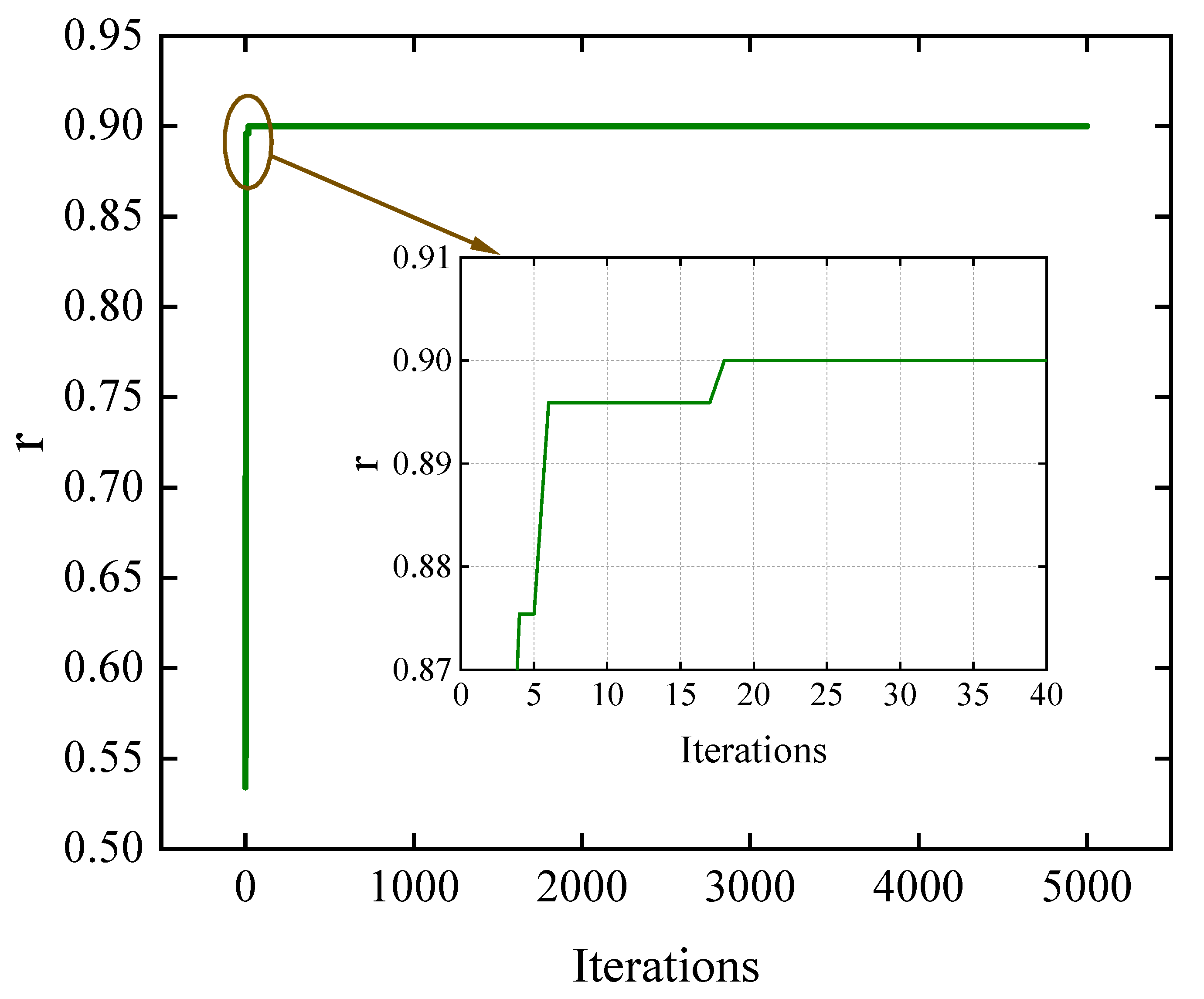
In the parameter initialization of BA, n = 10, A0 = 0.9, r0 = 0.9, Qmax = 1, Qmin = 0, α = 0.9, γ = 0.9, the max number of iterations N was 5000. The fitness function of the bat is the objective function, expressed by the root MSE (RMSE) of Equation (17), where T is the output of the training set, G is the sample size, and Y can be calculated using Equation (18):
5. Results and Discussion
5.1. Results
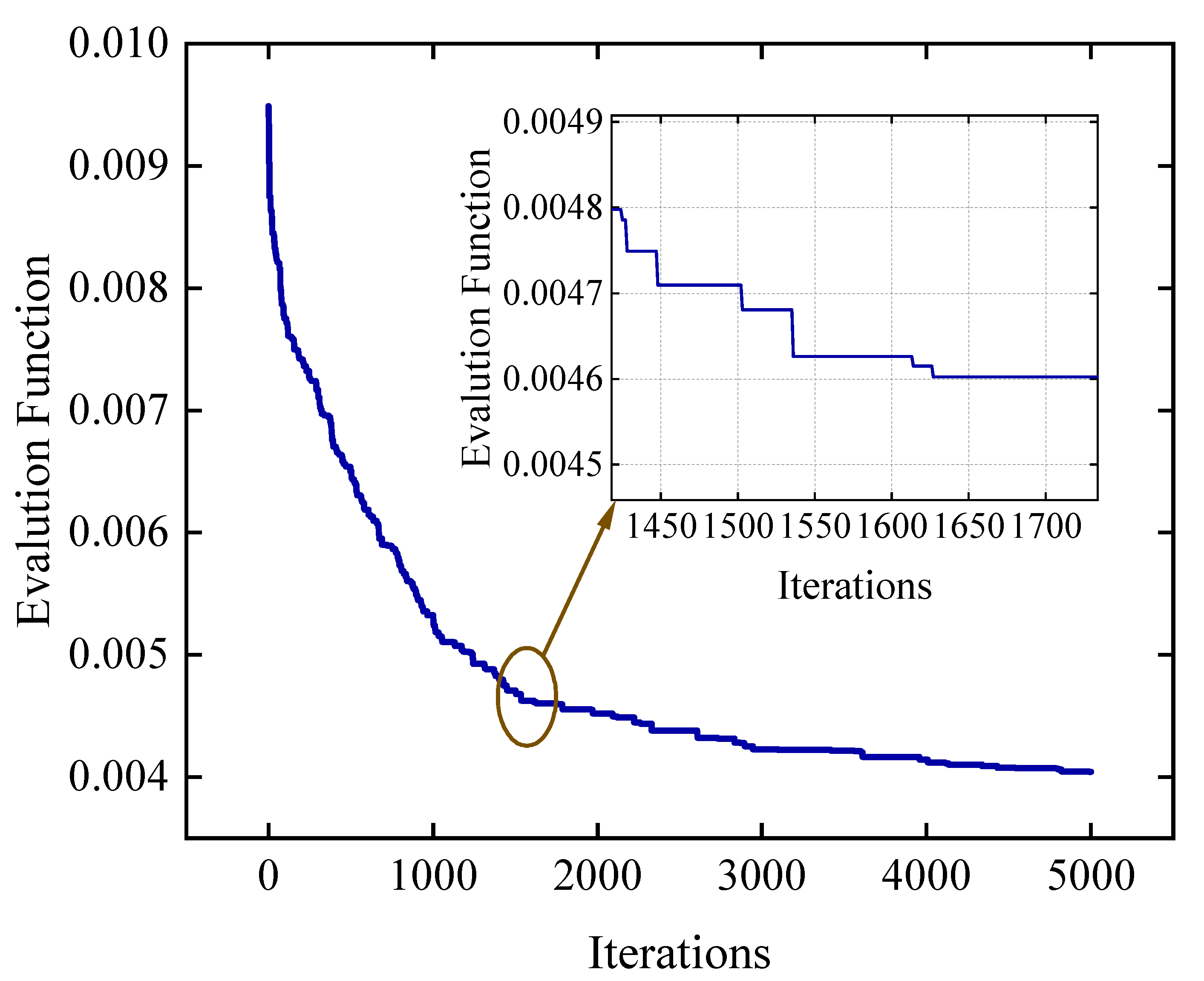
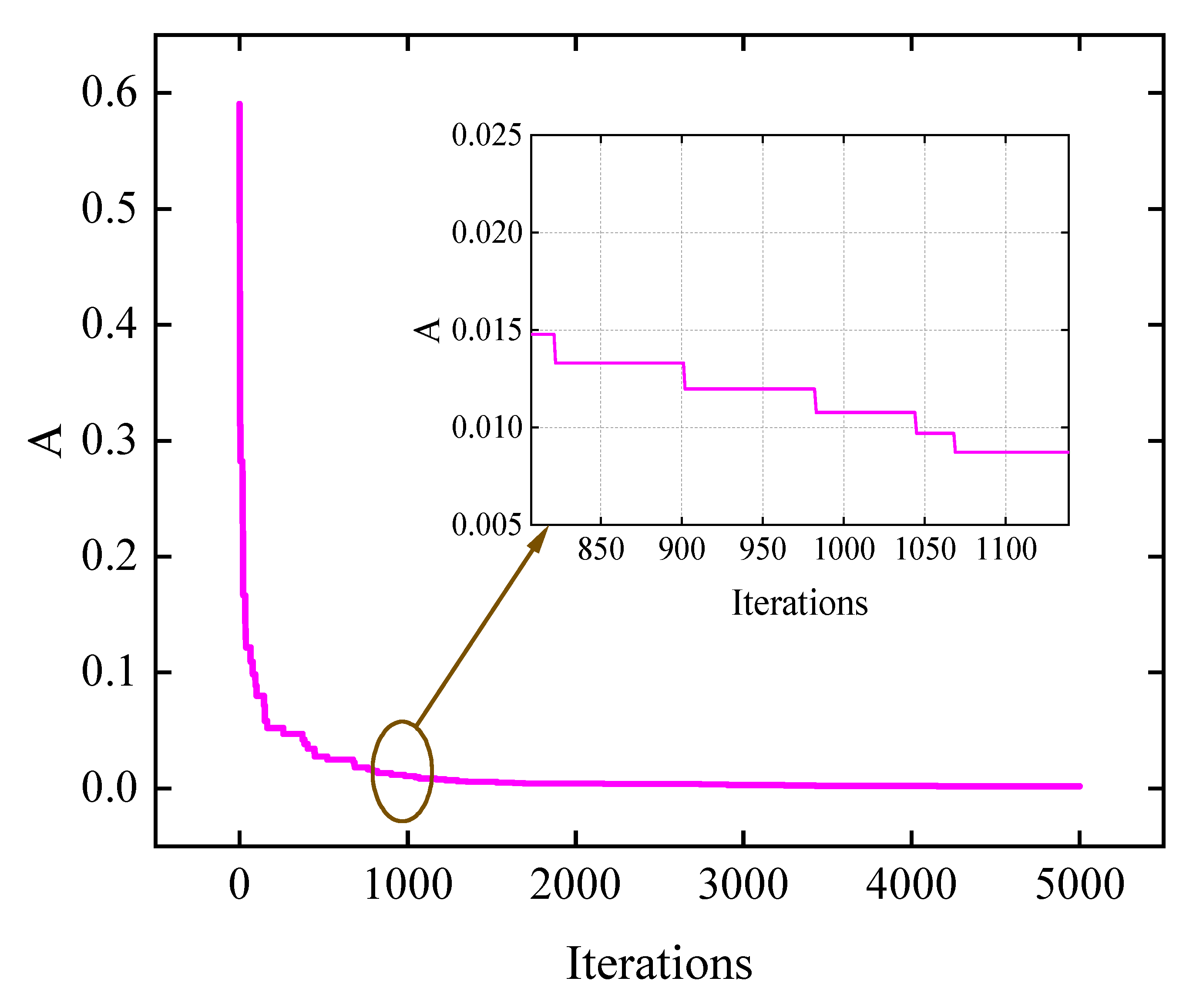
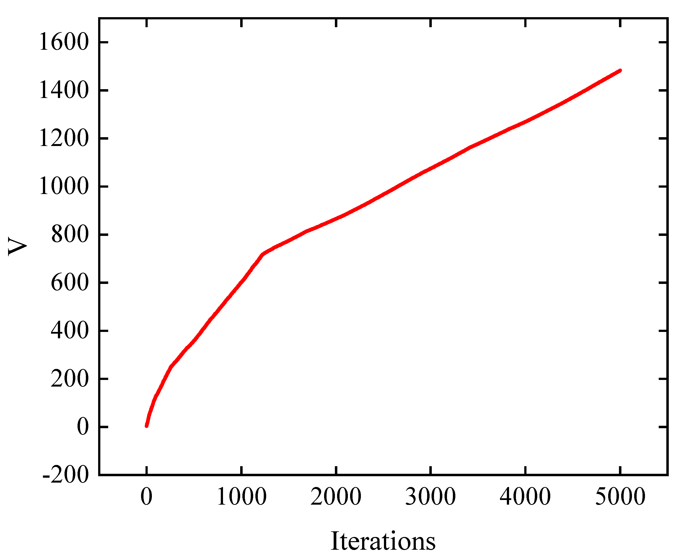
To analyze the optimization effect of the BA, we drew the evaluation function, impulse loudness, and impulse emission rate diagrams, as shown in Figure 12, Figure 13 and Figure 14. The evaluation function is fmin, representing the bat with the smallest current fitness level, and it was obtained using Equation (8). In this study, the bat’s velocity is a vector. Therefore, we propose a new concept, i.e., the average velocity modulus length . We first calculated the velocity modulus length of each bat, as shown in Equation (19), where D is the dimension of the vector. Then, the current average velocity modulus length of all the bats was calculated, as shown in Equation (20), where n is the number of bats. The relationship between the average velocity modulus length and number of iterations is shown in Figure 15.
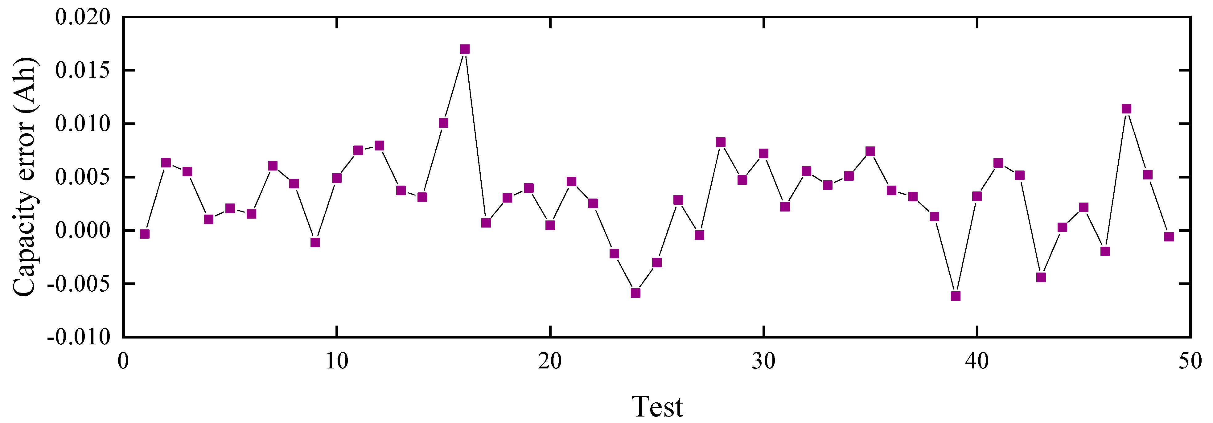
By analyzing Figure 12, we found that the value of the evaluation function dropped significantly. When the number of iterations was 1650, the evaluation function tended to converge, indicating that the BA achieved the expected effect of optimization. In Figure 13 and Figure 14, we can find that the impulse loudness Ai decreased during the iteration and reached the minimum at about 1100 iterations. The impulse emission rate ri increased and reached the maximum at about 18 iterations. Figure 15 shows that the average velocity modulus length of bats increased during the iteration. Combined with Figure 12, it can be concluded that the smaller the evaluation function, the better the position of the bat, and the closer the bat is to the position of the prey, the greater the bat’s velocity modulus. This is consistent with the fact that the closer the hunter is to the prey, the faster the hunter’s reaction speed is in nature. Figure 16 shows the test error result of the actual remaining capacity of the battery. The estimated error of the actual remaining capacity estimated by BA-ELM is less than 0.02 Ah, and the maximum error is less than 1%.
5.2. Discussion
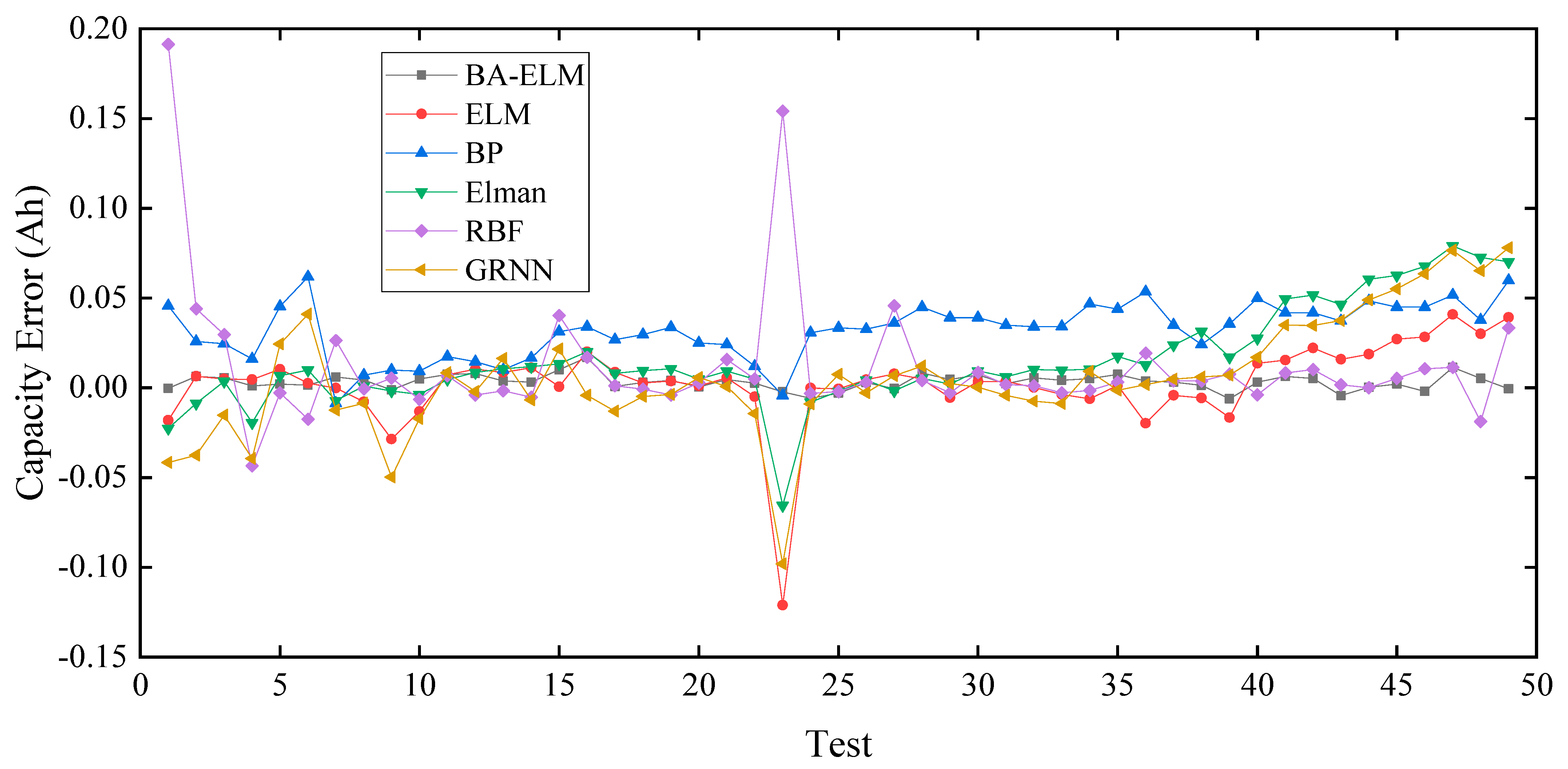
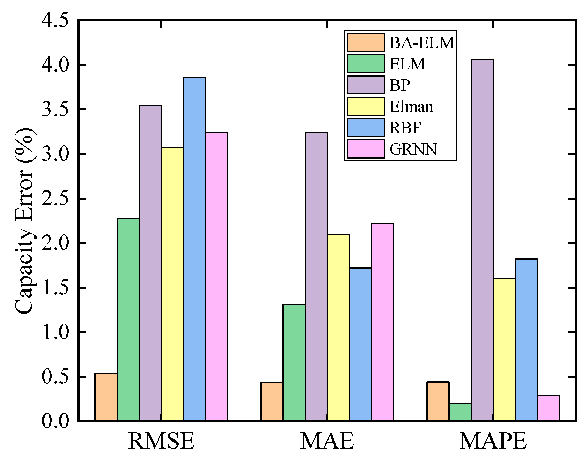
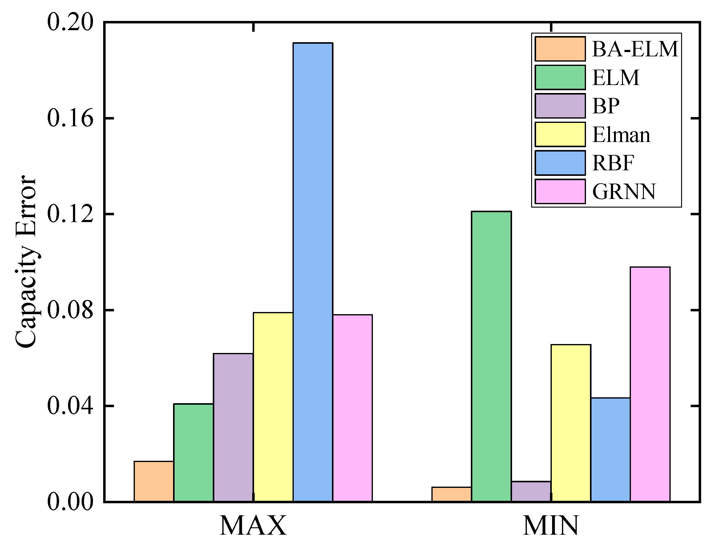
To further evaluate the estimation accuracy of the Caged of the BA-ELM model, we constructed neural network models of ELM, BP, Elman, RBF, and GRNN. The estimated error of the Caged, RMSE, mean absolute error (MAE), mean absolute percentage error (MAPE), MAX error (MAX), and MIN error (MIN) were used to compare the estimated accuracies of six models. The results are shown in Figure 17, Figure 18 and Figure 19 and Table 6 and Table 7.
The RMSE and MAE of the BA-ELM model are 0.5354% and 0.4326%, respectively. The RMSE of the other 5 models is between 2% and 4%, and the MAE is between 1% and 4%. The MAPE of the BP model is the largest, reaching 4.06%, and the MAPEs of BA-ELM, ELM, and GRNN are 0.44%, 0.20%, and 0.29%, respectively. The maximum error of the SOH result estimated by RBF is 0.1913 Ah, and the maximum error of the SOH result estimated by BA-ELM is only 0.017 Ah. The minimum error of the result of ELM estimation is 0.1212 Ah, and the minimum error of the result of BA-ELM estimation is only 0.062 Ah. Compared with the other five models, the results of the BA-ELM estimation show a smaller RMSE, MAE, MAX, and MIN.
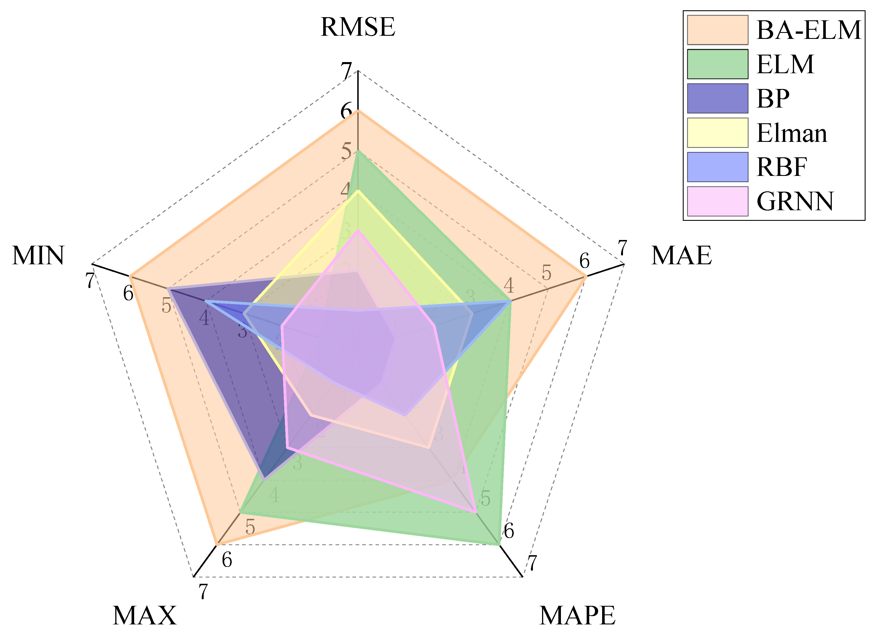
To further compare the performance of the six models on various error indicators, we sorted them according to the pros and cons of each indicator. Furthermore, we assigned 6 points for ranking first, 5 points for ranking second, and so on, with 1 point assigned for ranking sixth. The higher the score of a certain model on a certain error index, the better the performance of the algorithm on this error index. The results are shown in Table 8. We drew the radar chart of the 5 error indicators for the 6 models, and the results are shown in Figure 20. The shadow area covered by the BA-ELM model is the largest while the shadow area covered by BP and RBF is smaller. According to the total score of the five error indicators, the results of all models are as follows:
BA-ELM (28) > ELM (21) > Elman (15) = GRNN (15) > BP (13) > RBF (12).
Table 6.
Comprehensive comparison table of RMSE, MAE, and MAPE.
| Method | RMSE | MAE | MAPE |
|---|---|---|---|
| BA-ELM | 0.5354 | 0.4326 | 0.44 |
| ELM | 2.2713 | 1.3106 | 0.20 |
| BP | 3.5394 | 3.2429 | 4.06 |
| Elman | 3.0750 | 2.0936 | 1.60 |
| RBF | 3.8609 | 1.7217 | 1.82 |
| GRNN | 3.2439 | 2.2230 | 0.29 |
Table 7.
Comprehensive comparison table of MAX and MIN.
| Method | MAX | MIN |
|---|---|---|
| BA-ELM | 0.0170 | −0.0062 |
| ELM | 0.0409 | −0.1212 |
| BP | 0.0619 | −0.0086 |
| Elman | 0.0790 | −0.0656 |
| RBF | 0.1913 | −0.0434 |
| GRNN | 0.0780 | −0.0980 |
Table 8.
Scores of the six models.
| Method | RMSE | MAE | MAPE | MAX | MIN |
|---|---|---|---|---|---|
| BA-ELM | 6 | 6 | 4 | 6 | 6 |
| ELM | 5 | 4 | 6 | 5 | 1 |
| BP | 2 | 1 | 1 | 4 | 5 |
| Elman | 4 | 3 | 3 | 2 | 3 |
| RBF | 1 | 4 | 2 | 1 | 4 |
| GRNN | 3 | 2 | 5 | 3 | 2 |
Figure 20.
Radar chart of the statistical error of each model.

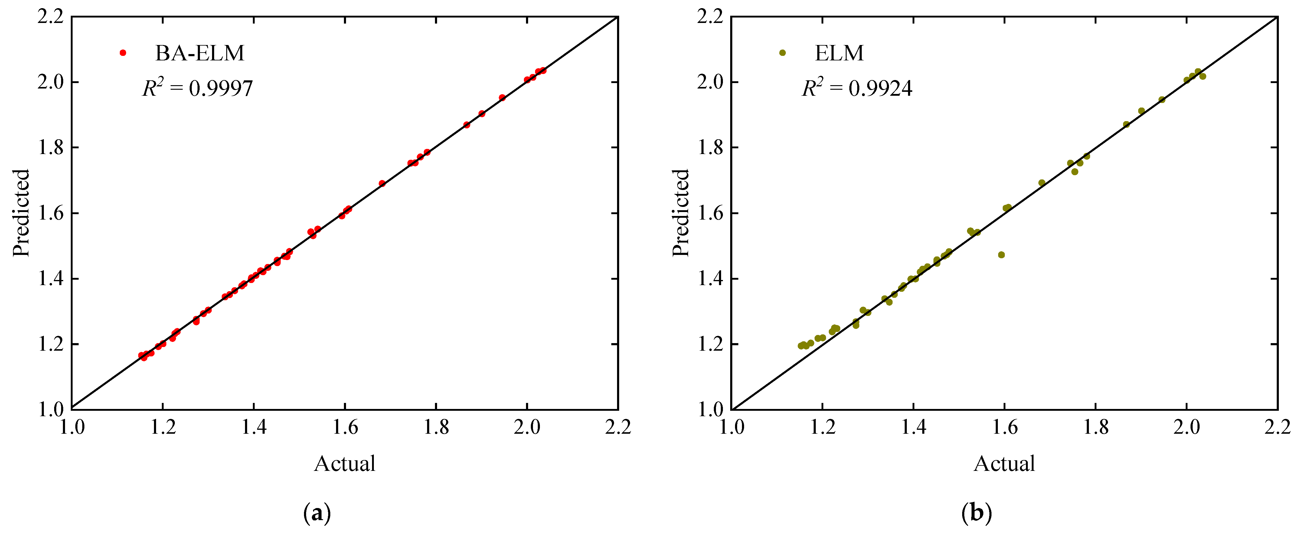
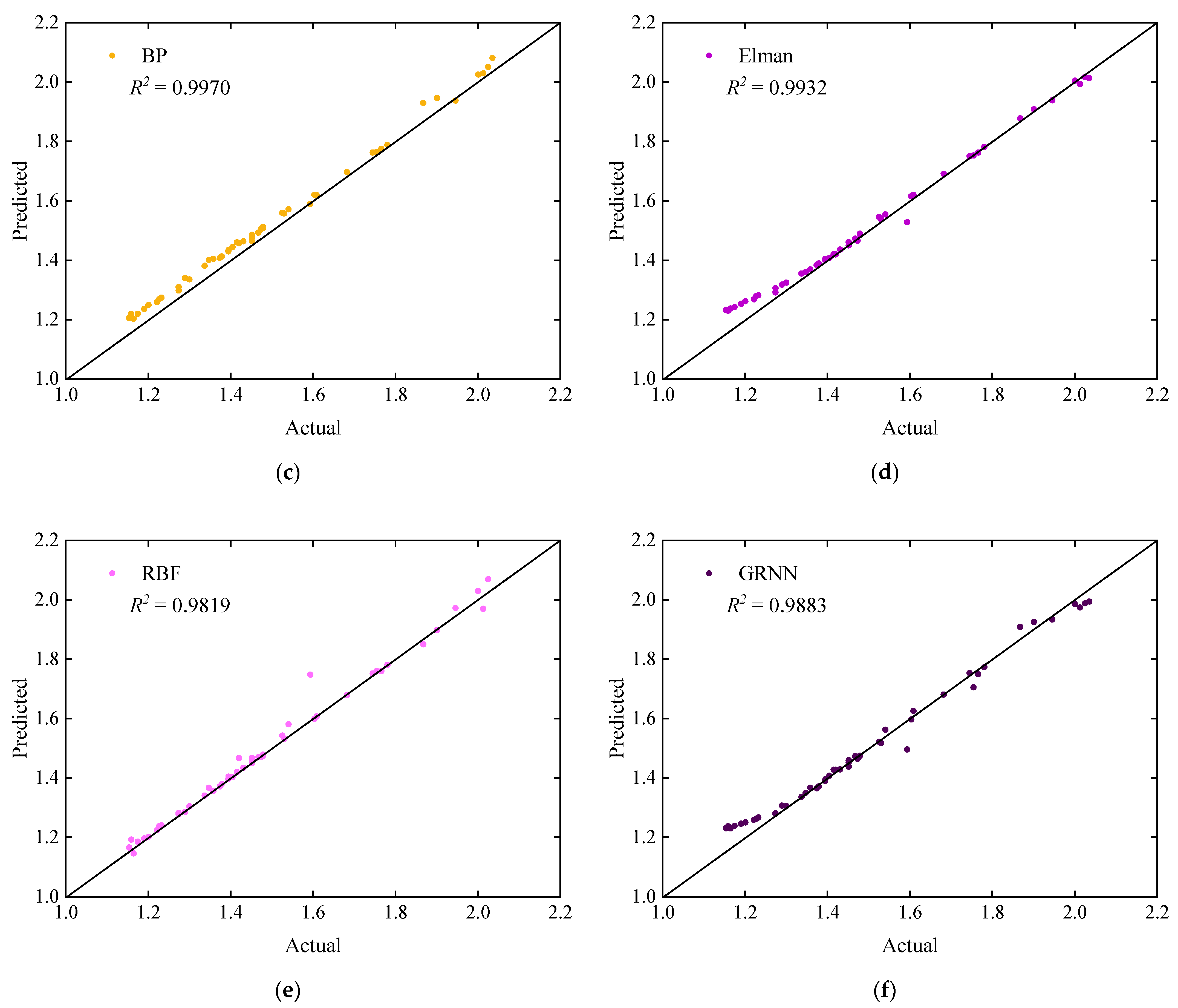
The predictive results of all models are illustrated in Figure 21a–f in the form of scatter plots and determination coefficients. It can be seen from the scatter plots that the BA-ELM provides less scattered estimates. Compared to other models, the fit line equation of BA-ELM is closer to the exact line (y = x), with a higher determination coefficient. It is followed by the ELM, BP, and Elman models. RBF and GRNN provide poor estimates while these two models also have lower determination coefficients of 0.9819 and 0.9883, respectively.
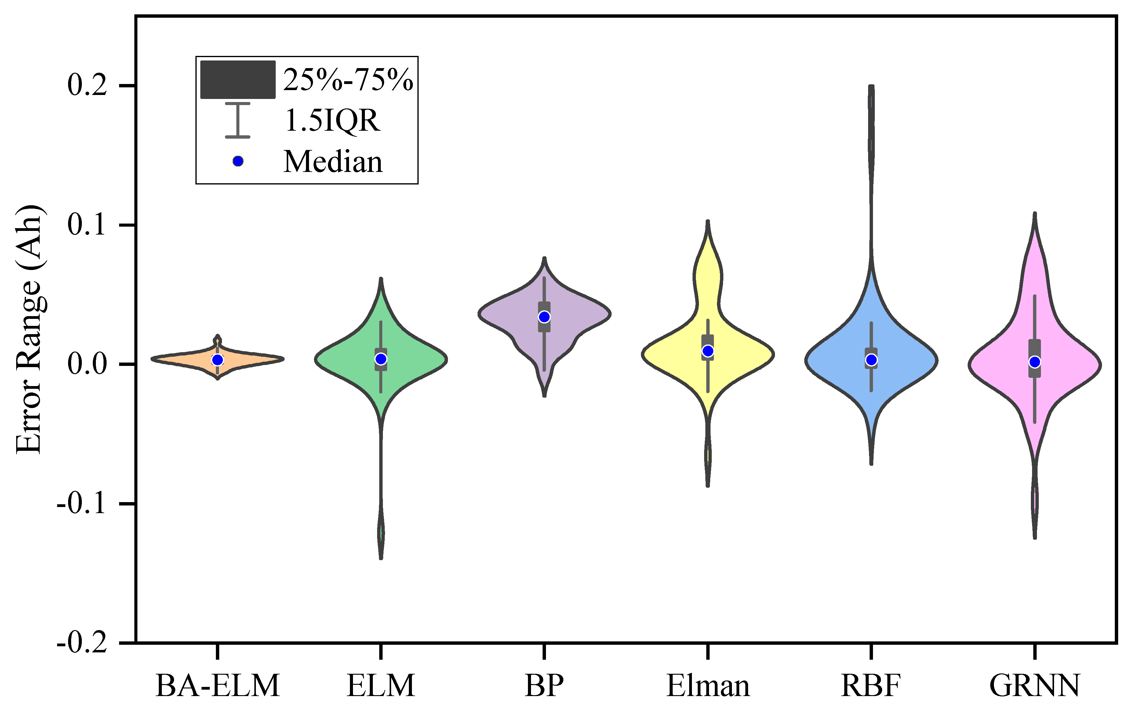
In Figure 22, from the violin diagrams, the BA-ELM model demonstrates its advantage by having a distribution that is a more similar distribution to the actual capacity as compared to other models. The data in the BA-ELM model is the most concentrated. A small amount of data in the ELM and RBF models, respectively, is far from the actual value. The median in the BP model is on the high side. A graphical comparison justifies the results obtained using the statistical indicators presented in the previous tables. Based on the above discussion, it can be concluded that compared with the other five models, the BA-ELM model has a better performance and can accurately estimate the actual remaining capacity and SOH of the battery.
6. Conclusions
This study creatively established the BA-ELM model, i.e., by simulating the echolocation hunting behavior of bats, searching for the global optimal solution, and optimizing the output connection weight, input connection weight, and value of bias of the ELM. This model was also used for the first time in the field of SOH estimation of lithium-ion batteries. Six neural network models of ELM, BP, Elman, RBF, GRNN, and BA-ELM were constructed, and the actual available capacity of the battery was estimated and compared through the test set.
The following conclusions can be derived based on the results and application:
- The relevant data of the battery can be analyzed by Pearson and Spearman correlation. The training time of the neural network model can be reduced by removing input variables with a low absolute value of Pearson’s and Spearman’s correlation coefficient.
- The value of the evaluation function dropped significantly using BA. The convergence speed was fast. The BA achieved the expected effect of optimization. We proposed a new concept, i.e., the average velocity modulus length. The bat’s velocity modulus became larger during the iteration. This is consistent with the fact in nature.
- The main advantages of the proposed BA-ELM model include a fast learning speed and high SOH estimation accuracy. The BA-ELM provided less scattered estimates, and its fit line equation was closer to the exact line (y = x) with a higher determination coefficient compared to other models. The connection weight and threshold of ELM were randomly set, which may cause the battery SOH estimation to be inaccurate. A globally optimized BA can be used to optimize the connection weights and bias of the ELM neural network.
- The RMSE of the BA-ELM model is 0.5354%, and the MAE is 0.4326%, which is the smallest among the 6 models. The RMSE values of the other model is 2.27%, 3.53%, 3.07%, 3.86%, and 3.24%, respectively. The estimated error of the actual battery capacity estimated using BA-ELM is less than 0.02 Ah, and the maximum error is less than 1%. Compared with the other five models, the results of BA-ELM estimation show a smaller RMSE, MAE, MAX, and MIN. It can be concluded that the estimation of the actual remaining capacity of the battery through the BA-ELM model has high accuracy and feasibility, which also makes the model have a good application prospect in the field of battery SOH.
Although the BA-ELM model provided promising results for estimating SOH of lithium-ion batteries, this study still has some limitations. The main limitations of this study and possible recommendations based on these limitations are listed below:
- In this study, the proposed model was only verified on a smaller dataset containing 165 cycles. Therefore, in the future, the performance of this model should be evaluated on larger data samples.
- The ELM model can be combined with other optimization algorithms to form a new hybrid model. Therefore, in the future, BA-ELM can be further validated and compared with other hybrid ELM models.
- Recently, some other variants of the ELM model have been successfully exploited, such as OSELM and OP-ELM. In the future, BA can be used with these advanced variants of ELM models.
- In this study, the impulse emission rate increased and reached the maximum at about 18 iterations. The change law of the loudness and pulse emission rate of the standard BA did not completely fit the actual application. The rates of pulse emission and loudness can be varied in a more sophisticated manner during the iteration. This also needs to be further studied in the future.
Author Contributions
Conceptualization, D.G., Z.Z. and Z.W.; methodology, D.G. and Z.Z.; software, D.G.; validation, D.G. and Z.Z.; formal analysis, D.G., X.K. and Z.Z.; investigation, D.G.; resources, D.G., Z.W. and Z.Z.; data curation, D.G.; writing—original draft preparation, D.G., X.K. and Z.Z.; writing—review and editing, D.G. and Z.Z.; supervision, Z.Z.; project administration, Z.Z. and Z.W.; funding acquisition, Z.W. and Z.Z. All authors have read and agreed to the published version of the manuscript.
Funding
This work is supported by the China Zhejiang Public Welfare Technology Application Research Project under Grant No. LGG19E070006, the National Natural Science Foundation of China under Grant No. 52107226, the China Postdoctoral Science Foundation under Grant No. 2020TQ0167, and the China Shaoxing Higher Education Teaching Reform Project under Grant No. SXSJG202120.
Institutional Review Board Statement
Not applicable.
Informed Consent Statement
Not applicable.
Data Availability Statement
Not applicable.
Acknowledgments
The authors would like to thank the reviewers for their comments and suggestions.
Conflicts of Interest
The authors declare no conflict of interest.
Nomenclature
| SOH | State of Health |
| ELM | Extreme Learning Machine |
| BA | Bat Algorithm |
| BA-ELM | Bat algorithm-Extreme Learning Machine |
| BP | Back Propagation |
| RBF | Radial Basis Function |
| GRNN | General Regression Neural Network |
| RMSE | Root Mean Square Error |
| MAE | Mean Absolute Error |
| SOC | State of Charge |
| OCV | Open-Circuit Voltage |
| EIS | Electrochemical Impedance Spectroscopy |
| ECM | Equivalent Circuit Model |
| SVM | Support Vector Machine |
| MAPE | Mean Absolute Percentage Error |
| MAX | MAX error |
| MIN | MIN error |
References
- Xuan, D.; Shi, Z.; Chen, J.; Zhang, C.; Wang, Y. Real-time estimation of state-of-charge in lithium-ion batteries using improved central difference transform method. J. Clean. Prod. 2020, 252, 787–797. [Google Scholar] [CrossRef]
- Lai, X.; He, L.; Wang, S.; Zhou, L.; Zhang, Y.; Sun, T. Co-estimation of state of charge and state of power for lithium-ion batteries based on fractional variable-order model. J. Clean. Prod. 2020, 255, 203–216. [Google Scholar] [CrossRef]
- Hsu, C.; Xiong, R.; Chen, N.; Li, J.; Tsou, N. Deep neural network battery life and voltage prediction by using data of one cycle only. Appl. Energy 2022, 306, 134–144. [Google Scholar] [CrossRef]
- He, H.; Xiong, R.; Guo, H. Online estimation of model parameters and state-of-charge of LiFePO4 batteries in electric vehicles. Appl. Energy 2012, 89, 413–420. [Google Scholar] [CrossRef]
- Zheng, Y.; Ouyang, M.; Li, X.; Lu, L.; Li, J.; Zhou, L.; Zhang, Z. Recording frequency optimization for massive battery data storage in battery management systems. Appl. Energy 2016, 183, 380–389. [Google Scholar] [CrossRef]
- Ge, D.; Zhang, Z.; Kong, X.; Wan, Z. Online SoC estimation of lithium-ion batteries using a new sigma points Kalman filter. Appl. Sci. 2021, 11, 11797. [Google Scholar] [CrossRef]
- Kong, X.; Plett, G.L.; Trimboli, M.S.; Zhang, Z.; Qiao, D.; Zhao, T.; Zheng, Y. Pseudo-two-dimensional model and impedance diagnosis of micro internal short circuit in lithium-ion cells. J. Energy Storage 2020, 27, 101085. [Google Scholar] [CrossRef]
- Weng, C.; Sun, J.; Peng, H. A unified open-circuit-voltage model of lithium-ion batteries for state-of-charge estimation and state-of-health monitoring. J. Power Sources 2014, 258, 228–237. [Google Scholar] [CrossRef]
- Galeotti, M.; Cina, L.; Giammanco, C.; Cordiner, S.; Di, C. Performance analysis and SOH (state of health) evaluation of lithium polymer batteries through electrochemical impedance spectroscopy. Energy 2015, 89, 678–686. [Google Scholar] [CrossRef]
- Swierczynski, M.; Stroe, D.; Stanciu, T.; Kær, S.K. Electrothermal impedance spectroscopy as a cost efficient method for determining thermal parameters of lithium ion batteries: Prospects, measurement methods and the state of knowledge. J. Clean. Prod. 2017, 155, 63–71. [Google Scholar] [CrossRef]
- Xiong, R.; Sun, F.; Chen, Z.; He, H. A data-driven multi-scale extended Kalman filtering based parameter and state estimation approach of lithium-ion polymer battery in electric vehicles. Appl. Energy 2014, 113, 463–476. [Google Scholar] [CrossRef]
- Saxena, S.; Xing, Y.; Kwon, D.; Pecht, M. Accelerated degradation model for C-rate loading of lithium-ion batteries. J. Electr. Power Energy Syst. 2019, 107, 438–445. [Google Scholar] [CrossRef]
- Mastali, M.; Farhad, S.; Farkhondeh, M.; Fraser, R.; Fowler, M. Simplified electrochemical multi-particle model for LiFePO4 cathodes in lithium-ion batteries. J. Power Sources 2015, 275, 633–643. [Google Scholar] [CrossRef]
- Li, J.; Cheng, Y.; Jia, M.; Tang, Y.; Lin, Y.; Zhang, Z.; Liu, Y. An electro chemical thermal model based on dynamic responses for lithium iron phosphate battery. J. Power Sources 2014, 255, 130–143. [Google Scholar] [CrossRef]
- Cheng, G.; Wang, X.; He, Y. Remaining useful life and state of health prediction for lithium batteries based on empirical mode decomposition and a long and short memory neural network. Energy 2021, 232, 22–32. [Google Scholar] [CrossRef]
- Kristen, A.; Peter, M. Data-driven prediction of battery cycle life before capacity degradation. Nat. Energy 2019, 4, 383–391. [Google Scholar]
- Deng, Y.; Ying, H.; Zhu, J.; Wei, K.; Chen, J.; Zhang, F.; Liao, G. Feature parameter extraction and intelligent estimation of the State-of-Health of lithium-ion batteries. Energy 2019, 176, 91–102. [Google Scholar] [CrossRef]
- Shen, S.; Sadoughi, M.; Chen, X.; Hong, M.; Hu, C. A deep learning method for online capacity estimation of lithium-ion batteries. J. Energy Storage 2019, 25, 100817. [Google Scholar] [CrossRef]
- Chen, Z.; Sun, M.; Shu, X.; Xiao, R.; Shen, J. Online state of health estimation for lithium-ion batteries based on support vector machine. Appl. Sci. 2018, 8, 925. [Google Scholar] [CrossRef] [Green Version]
- Tian, J.; Xiong, R.; Shen, W.; Wang, J.; Yang, R. Online simultaneous identification of parameters and order of a fractional order battery model. J. Clean. Prod. 2019, 247, 119147. [Google Scholar] [CrossRef]
- Yang, D.; Wang, Y.; Pan, R.; Chen, R.; Chen, Z. A neural network based state-of-health estimation of lithium-ion battery in electric vehicles. Energy Procedia 2017, 105, 2059–2064. [Google Scholar] [CrossRef]
- Li, P.; Zhang, Z.; Xiong, Q.; Ding, B.; Hou, J.; Luo, D. State-of-health estimation and remaining useful life prediction for the lithium-ion battery based on a variant long short term memory neural network. J. Power Sources 2020, 459, 228069. [Google Scholar] [CrossRef]
- Hossain, M.; Mahammad, A.; Hussain, A.; Mohamad, H.; Ayob, A.; Mohammad, N. Extreme learning machine model for state-of-charge estimation of lithium-ion battery using gravitational search algorithm. IEEE Trans. Ind. Appl. 2019, 55, 4225–4234. [Google Scholar] [CrossRef]
- Luo, X.; Sun, J.; Wang, L.; Wang, W.; Zhao, W.; Wu, J. Short-term wind speed forecasting via stacked extreme learning machine with generalized correntropy. IEEE Trans. Ind. Infor. 2018, 14, 4963–4971. [Google Scholar] [CrossRef] [Green Version]
- Liu, M.; Zhao, N.; Li, J.; Victor, C. Spectrum sensing based on maximum generalized correntropy under symmetric alpha stable noise. IEEE Trans. Veh. Technol. 2019, 68, 262–266. [Google Scholar] [CrossRef]
- Li, S.; He, H.; Li, J. Big data driven lithium-ion battery modeling method based on SDAE-ELM algorithm and data pre-processing technology. Appl. Energy 2019, 242, 1259–1273. [Google Scholar] [CrossRef]
- Wang, X.; Sun, Q.; Kou, X.; Ma, W.; Zhang, H.; Liu, R. Noise immune state of charge estimation of li-ion battery via the extreme learning machine with mixture generalized maximum correntropy criterion. Energy 2022, 239, 406–420. [Google Scholar] [CrossRef]
- Chen, L.; Wang, H.; Liu, B.; Wang, Y.; Ding, Y.; Pan, H. Battery state-of-health estimation based on a metabolic extreme learning machine combining degradation state model and error compensation. Energy 2021, 215, 78–88. [Google Scholar] [CrossRef]
- Ma, Y.; Wu, L.; Guan, Y.; Peng, Z. The capacity estimation and cycle life prediction of lithium-ion batteries using a new broad extreme learning machine approach. J. Power Sources 2020, 476, 228581. [Google Scholar] [CrossRef]
- Mariani, V.; Och, S.; Coelho, L.; Domingues, E. Pressure prediction of a spark ignition single cylinder engine using optimized extreme learning machine models. Appl. Energy 2019, 249, 204–221. [Google Scholar] [CrossRef]
- Adnan, R.; Mostafa, R.; Kisi, O.; Yaseen, Z.; Shahid, S.; Zounemat-Kermani, M. Improving streamflow prediction using a new hybrid ELM model combined with hybrid particle swarm optimization and grey wolf optimization. Knowl. Based Syst. 2021, 230, 10739. [Google Scholar] [CrossRef]
- Bardhan, A.; Samui, P.; Ghosh, K.; Gandomi, A.; Bhattacharyya, S. ELM-based adaptive neuro swarm intelligence techniques for predicting the California bearing ratio of soils in soaked conditions. Appl. Soft Comput. 2021, 110, 107595. [Google Scholar] [CrossRef]
- Hasançebi, O.; Teke, T.; Pekcan, O. A bat-inspired algorithm for structural optimization. Comput. Struct. 2013, 128, 77–90. [Google Scholar] [CrossRef]
- Bahmani-Firouzi, B.; Azizipanah-Abarghooee, R. Optimal sizing of battery energy storage for micro-grid operation management using a new improved bat algorithm. Electr. Power Energy Syst. 2014, 56, 42–54. [Google Scholar] [CrossRef]
- Pan, Z.; Quynh, N.; Ali, Z.; Dadfar, S.; Kashiwagi, T. Enhancement of maximum power point tracking technique based on PV-Battery system using hybrid BAT algorithm and fuzzy controller. J. Clean. Prod. 2020, 274, 719–734. [Google Scholar] [CrossRef]
- Yang, Q.; Dong, N.; Zhang, J. An enhanced adaptive bat algorithm for microgrid energy scheduling. Energy 2021, 232, 121014–121030. [Google Scholar] [CrossRef]
- Shivaie, M.; Mokhayeri, M.; Kiani-Moghaddam, M.; Ashouri-Zadeh, A. A reliability-constrained cost-effective model for optimal sizing of an autonomous hybrid solar/wind/diesel/battery energy system by a modified discrete bat search algorithm. Sol. Energy 2019, 189, 344–356. [Google Scholar] [CrossRef]
- Peddakapu, K.; Mohamed, M.; Srinivasarao, P.; Leung, P. Frequency stabilization in interconnected power system using bat and harmony search algorithm with coordinated controllers. Appl. Soft Comput. 2021, 113, 107986. [Google Scholar] [CrossRef]
- Huang, G.; Zhu, Q.; Siew, C. Extreme learning machine: Theory and applications. Neurocomputing 2006, 70, 489–501. [Google Scholar] [CrossRef]
- Yang, X. A new metaheuristic Bat-inspired Algorithm. Stud. Comput. Intell. 2010, 284, 65–74. [Google Scholar]
- NASA Prognostic Center of Excellence. Available online: https://ti.arc.nasa.gov/tech/dash/groups/pcoe/prognostic-data-repository/#algae (accessed on 1 March 2021).
Figure 1.
Neural network structure of ELM.

Figure 2.
Echolocation hunting of the bat.

Figure 3.
Relationship between the actual remaining capacity and cycles.

Figure 4.
Scatter figure of TI.

Figure 5.
Scatter figure of TV.

Figure 6.
Scatter figure of Ttotal,charge.

Figure 7.
Scatter figure of Ttotal,discharge.

Figure 8.
Scatter figure of ΔTempdischarge.

Figure 9.
Scatter figure of ΔVcharge.

Figure 10.
Scatter figure of ΔVcharge.

Figure 11.
Algorithmic process of BA-ELM.

Figure 12.
Evaluation function.

Figure 13.
Impulse loudness.

Figure 14.
Impulse emission rate.

Figure 15.
Average velocity modulus length.

Figure 16.
Test error of actual remaining capacity estimation.

Figure 17.
Comparison of estimation errors of Caged of each model.

Figure 18.
Comparison of RMSE MAE and MAPE.

Figure 19.
Comparison of MAX and MIN.

Figure 21.
Capacity of actual vs predicted in the form of scatter plot and R2, respectively for: (a) BA-ELM; (b) ELM; (c) BP; (d) Elman; (e) RBF; (f) GRNN.
Figure 21.
Capacity of actual vs predicted in the form of scatter plot and R2, respectively for: (a) BA-ELM; (b) ELM; (c) BP; (d) Elman; (e) RBF; (f) GRNN.


Figure 22.
Violin diagram of six models.

Table 2.
Algorithmic process of BA.
| The Pseudo Code of Bat Algorithm |
|---|
| Step 1: Initialize parameter settings, including the population size n, initial impulse loudness A0, initial impulse emission rate r0, maximum frequency Qmax, minimum frequency Qmin, max number of iterations N, and fitness evaluation function Fitness (x). |
| Step 2: While (t < the max number of iterations) Calculate the frequency Qi, location Si, speed Vi, and fitness value Fitnessi of each bat. |
| Step 3: If (rand > ri) 1. Obtain an optimal solution BestS in this iteration. 2. Calculate the local solutions around the optimal solution. |
| Step 4: End if Produce new solutions by change randomly |
| Step 5: if (rand < Ai and Fitness (xi) < Fitness (x∗)). 1. Accept the new solutions. 2. Decrease the impulse loudness Ai and increase the impulse emission rate ri. |
| Step 6: End if Sort all bats and obtain the optimal solution BestS in this iteration. |
| Step 7: End while |
Table 3.
Judgment criteria between the degree of correlation and the correlation coefficient.
| The absolute value of the correlation coefficient | 0.8–1.0 | 0.6–0.8 | 0.4–0.6 | 0.2–0.4 | 0.0–0.2 |
| The degree of correlation | Very strong | Strong | Medium | Weak | Very weak |
Table 4.
Coefficient of Pearson and Spearman.
| TI | TV | Ttotal,charge | Ttotal,discharge | ΔTempdischarge | ΔVcharge | ΔVdischarge | |
|---|---|---|---|---|---|---|---|
| Pearson | 0.9969 | −0.9412 | −0.2589 | 0.9931 | 0.9710 | −0.9828 | −0.9567 |
| Spearman | 0.9986 | −0.91615 | −0.2202 | 0.9979 | 0.9579 | −0.9889 | −0.9619 |
Table 5.
The pseudo code of the proposed model.
| The Pseudo Code of BA-ELM |
|---|
| Step 1: Data acquisition and data processing. |
| Step 2: Generate the training set and the test set. |
| Step 3: Initialize the parameters of BA, including the population size n, initial impulse loudness A0, initial impulse emission rate r0, maximum frequency Qmax, minimum frequency Qmin, the max number of iterations N, and fitness evaluation function Fitness (x). |
| Step 4: While (t < the max number of iterations) Calculate the frequency Qi, location Si, speed Vi, fitness value Fitnessi of each bat. |
| Step 5: If (rand > ri) 1. Obtain an optimal solution BestS in this iteration. 2. Calculate the local solutions around the optimal solution. |
| Step 6: End if Produce new solutions by change randomly |
| Step 7: If (rand < Ai and Fitness (xi) < Fitness (x∗)). 1. Accept the new solutions. 2. Decrease the impulse loudness Ai and increase the impulse emission rate ri. |
| Step 8: End if Sort all bats and obtain the optimal solution BestS in this iteration. |
| Step 9: End while and accept the optimal output connection weight β. |
| Step 10: Determine the input connection weight ω and the bias b. Obtain the network structure of BA-ELM |
| Step 11: Estimate the actual battery capacity using the BA-ELM model. |
Publisher’s Note: MDPI stays neutral with regard to jurisdictional claims in published maps and institutional affiliations. |
© 2022 by the authors. Licensee MDPI, Basel, Switzerland. This article is an open access article distributed under the terms and conditions of the Creative Commons Attribution (CC BY) license (https://creativecommons.org/licenses/by/4.0/).
Share and Cite
MDPI and ACS Style
Ge, D.; Zhang, Z.; Kong, X.; Wan, Z. Extreme Learning Machine Using Bat Optimization Algorithm for Estimating State of Health of Lithium-Ion Batteries. Appl. Sci. 2022, 12, 1398. https://doi.org/10.3390/app12031398
AMA Style
Ge D, Zhang Z, Kong X, Wan Z. Extreme Learning Machine Using Bat Optimization Algorithm for Estimating State of Health of Lithium-Ion Batteries. Applied Sciences. 2022; 12(3):1398. https://doi.org/10.3390/app12031398
Chicago/Turabian StyleGe, Dongdong, Zhendong Zhang, Xiangdong Kong, and Zhiping Wan. 2022. "Extreme Learning Machine Using Bat Optimization Algorithm for Estimating State of Health of Lithium-Ion Batteries" Applied Sciences 12, no. 3: 1398. https://doi.org/10.3390/app12031398
Note that from the first issue of 2016, this journal uses article numbers instead of page numbers. See further details here.