
Short-Term Prediction of Bike-Sharing Demand Using Multi-Source Data: A Spatial-Temporal Graph Attentional LSTM Approach


1
School of Civil and Transportation Engineering, Hebei University of Technology, Tianjin 300401, China
2
School of Architecture and the Built Environment, Royal Institute of Technology (KTH), 11428 Stockholm, Sweden
3
School of Transportation, Southeast University, Dongnandaxue Road 2, Nanjing 211189, China
4
School of Architecture and Art Design, Hebei University of Technology, Tianjin 300401, China
*
Author to whom correspondence should be addressed.
Appl. Sci. 2022, 12(3), 1161; https://doi.org/10.3390/app12031161
Submission received: 1 December 2021
/
Revised: 8 January 2022
/
Accepted: 20 January 2022
/
Published: 23 January 2022
(This article belongs to the Topic Intelligent Transportation Systems)
Abstract
:As a convenient, economical, and eco-friendly travel mode, bike-sharing greatly improved urban mobility. However, it is often very difficult to achieve a balanced utilization of shared bikes due to the asymmetric spatio-temporal user demand distribution and the insufficient numbers of shared bikes, docks, or parking areas. If we can predict the short-run bike-sharing demand, it will help operating agencies rebalance bike-sharing systems in a timely and efficient way. Compared to the statistical methods, deep learning methods can automatically learn the relationship between the inputs and outputs, requiring less assumptions and achieving higher accuracy. This study proposes a Spatial-Temporal Graph Attentional Long Short-Term Memory (STGA-LSTM) neural network framework to predict short-run bike-sharing demand at a station level using multi-source data sets. These data sets include historical bike-sharing trip data, historical weather data, users’ personal information, and land-use data. The proposed model can extract spatio-temporal information of bike-sharing systems and predict the short-term bike-sharing rental and return demand. We use a Graph Convolutional Network (GCN) to mine spatial information and adopt a Long Short-Term Memory (LSTM) network to mine temporal information. The attention mechanism is focused on both temporal and spatial dimensions to enhance the ability of learning temporal information in LSTM and spatial information in GCN. Results indicate that the proposed model is the most accurate compared with several baseline models, the attention mechanism can help improve the model performance, and models that include exogenous variables perform better than the models that only consider historical trip data. The proposed short-term prediction model can be used to help bike-sharing users better choose routes and to help operators implement dynamic redistribution strategies.
1. Introduction
As an economical, convenient, and eco-friendly travel mode, bike-sharing systems have grown dramatically worldwide during the last decade [1]. The systems can help relieve air pollution and traffic congestion, and bring health benefits by involving more physical activities [2]. A bike-sharing system is an access/egress mode service for public transport. It supports multimodal transport connections and increases the reachable areas of public transit [3]. By March 2021, 2012 bike-sharing programs have been put in operation and 300 others are under construction around the world [4].
Bike-sharing systems can be categorized into the following two types: a docked bike-sharing system and dockless bike-sharing system [5]. The docked bike-sharing system has stationary docking stations for users to rent and return bikes. For the dockless bike-sharing system, riders can use mobile phone applications (APPs) to rent and return bikes in the designated physical or electric-fencing areas [6,7].
These two bike-sharing systems help promote urban mobility. However, because user demand distribution is asymmetric from a spatial and temporal perspective, shared bike distribution is unbalanced. In order to better satisfy user demand and assist operators in scheduling the optimal routes and rebalancing the timetable, it is necessary to accurately predict the short-run bike-sharing demand in advance to improve the efficacy of bike-sharing systems [8]. Users could better plan travel strategies and change the origins/destinations in advance, which will eventually help balance the systems without rebalancing the shared bikes. Furthermore, short-term predictive models could also be applied to design a dynamic redistribution strategy and better balance the shared bikes distribution between saturated and non-saturated stations/regions [9].
Previous studies mainly focus on the predictions of shared-bike usage at the city level [10], station cluster level [11], and station/grid level [10]. Although the bike-sharing usage aggregating at the city level and cluster level does simplify the problem, it neglects the characteristics of and interactions among stations and fails to extract spatial effects under fine-grained content. Therefore, the generated prediction models are unsatisfactorily reliable [10,12]. Therefore, accurate station-level demand prediction for docked bike-sharing and the TAZ/grid-level demand prediction for dockless bike-sharing will be better for operators of bike-sharing systems to rebalance the imbalanced supply of shared bikes and recommend stations to passengers [13]. Classical spatial regression includes spatial effects in the demand prediction process; however, it can be limited by assumptions, accuracy, and computer power. The Spatial-Temporal Graph Attentional Long Short-Term Memory (STGA-LSTM) neural network model proposed in this study incorporates spatial and temporal usage patterns to predict the short-run demand for docked shared bikes. Moreover, the attention mechanism is useful to improve the accuracy and interpretability of a deep-learning neural network [14]. As far as we know, it is one of the first efforts to integrate the GC-LSTM model with the attention mechanism for the prediction of short-term bike-sharing demand, and this method can be generalized for the demand prediction of both docked and dockless bike-sharing systems. To facilitate the training and testing of the proposed model, this paper uses smart card data of docked bike-sharing provided by the Nanjing public bicycle company, points of interest (POIs) data obtained by calling the Amap API [15], road network data downloaded from OpenStreetMap [16], and historical hourly weather data extracted from Weather Underground [17]. By comparing the proposed model with the leading prediction methods, it is shown that the proposed method is effective in predicting the short-run demand for shared bikes.
The study makes contributions mainly in the following aspects:
- A novel GC-LSTM model with spatio-temporal attentional matrices is proposed to predict the short-term demand for bike-sharing rental and return at the station level.
- Exogenous factors (e.g., weather information, POIs data, and users’ personal information) are considered in the prediction model.
- Comprehensive performance comparisons are performed based on real-world datasets.
The sections of this paper are constructed as follows. In Section 2, the literature on the prediction models for short-term demand of shared bikes is reviewed. In Section 3, the framework of the novel GC-LSTM model and each component are illustrated. Section 4 conducts experiments and discusses the results. The final section concludes this paper and proposes future research directions.
2. Literature Review
Short-run bike-sharing prediction assists system operators in daily operations and improves the system reliability and accessibility [18]. During the past decades, how to predict the short-term demand of bike-sharing has been widely studied. The methods for bike-sharing prediction can be divided into parametric methods and non-parametric methods.
The parametric methods usually regard bike-sharing demand prediction as a time-series issue from multi-source and heterogeneous data [19]. Auto-Regressive Moving Average (ARMA) model-based models were adopted to predict the short-term bike-sharing demand. Kaltenbrunner et al. [20] applied an ARMA model to predict available shared bikes for stations with a some minutes/hours horizon window ahead. Yoon et al. [21] proposed a modified Auto-Regressive Integrated Moving Average (ARIMA) model to forecast the number of available shared bikes for each station considering temporal factors of and interactions among stations. Gallop et al. [22] applied a Seasonal Auto-Regressive Integrated Moving Average (SARIMA) model to analyze bike-sharing demand using hourly bike usage and the corresponding weather data. They found that weather-related factors, especially temperature and rain, significantly impacted bike-sharing usage. Previous ARMA-based models can use temporal information to predict the bike-sharing demand. However, these models cannot well extract the heterogeneous correlations among stations [3].
The non-parametric methods include machine learning approaches and deep learning approaches. Using machine learning methods, several researchers worked to establish nonlinear prediction model based on massive bike-sharing historical trip data. A few studies adopted Random Forest [23], Bayesian network [24], Gradient Boosted Tree [25], and Artificial Neural Networks (ANN) [26] to predict the bike-sharing demand at each station at any given time period in the future, without including the spatial or temporal correlations between stations.
In addition, recent studies used deep learning methods to predict the short-term station-level bike-sharing demand. Wang and Kim [27] applied Long Short-Term Memory (LSTM) neural networks and Gated Recurrent Unit (GRU) to predict the short-term availability of shared bikes at docking stations using historical data within one month. Chen et al. [28] proposed the Recurrent Neural Network (RNN) to predict both rental and return demand for every station in the system using time, weather, and station data. Zhang et al. [29] adopted the LSTM model to predict the short-term bike-sharing usage by considering the correlation between bike-sharing users and public transport passengers. To extract spatial-temporal dependencies, some studies combined both network structures and put forward a Convolutional LSTM network (Conv-LSTM). For example, Du et al. [12] combined irregular CNN and LSTM units and used historical passenger flows and external factors such as weather, traffic control, and social activities to explore the characteristic of spatial-temporal traffic flows and predict hourly road traffic flows. Ai et al. [30] proposed a Conv-LSTM model and predicted the dockless bike-sharing systems distribution within a short-run period by considering spatial-temporal variables. Xu et al. [31] constructed a Multi-Block Hybrid model by involving CNN and GRU to implement short-run dockless bike-sharing prediction. Furthermore, Graph Neural Network (GCN) could detect the complex heterogeneous spatio-temporal effects of bike-sharing ridership, by treating the bike station as the vertices. San Kim et al. [32] developed a Graph Neural Network (GCN) prediction model and estimated the bike-sharing demand in different hours of a day for each station by considering the temporal patterns, spatial characteristics, and global variables (weather and weekday/weekend). Pandya [33] applied spatio-temporal GCN (ST-GCN) to predict shared bike flows across all stations in the next hour. Guo et al. [34] built an ST-GCN to simulate bike-sharing demand at the city level. They used GCN to explore the spatial connection and GRU to explore the temporal dependency. Yoshida et al. [35] put forward a relational GCN-based method for the prediction of the station-level demand. Chai et al. [36] developed a multi-Graph Convolutional LSTM (GC-LSTM) network for prediction of bike-flow at the station level by catching the heterogeneous inter-station spatial relationships. Recently, attention mechanism has been incorporated in the convolutional network to predict bike-sharing demand, which has been proven to improve the accuracy and interpretability of deep learning algorithms [12,13,14]. Zhou et al. [37] divided the entire city into multiple regions and predicted the multi-step city-wide demand of Didi, taxi, and bike-sharing at the region level by applying attention mechanism in neural network models.
In conclusion, deep learning has proven to be an effective tool for bike-sharing prediction and numerous research studies have applied combined prediction methods of deep learning to improve the prediction outcome. However, insufficient research has been done regarding incorporating the advantages of GCN, LSTM, and the attention mechanism. Furthermore, none of the aforementioned studies established an attention-based GC-LSTM for the prediction of short-run docked bike-sharing demand at the station level. To fill the aforementioned research gaps, a novel GC-LSTM model with the attention mechanism has been proposed to predict short-run bike-sharing demand based on multi-source data. The station-level shared-bike demand is influenced by multiple complex factors [32,38,39,40]. The data sets considered the multi-source heterogeneous information, including weather conditions, land-use data around the bike station, and users’ personal information.
3. Methodology
This section elaborates every preliminary methodology covered by the proposed model, including the LSTM model, GCN model, and attention mechanism. Then, the proposed Spatial-Temporal Graph Attentional LSTM (STGA-LSTM) model is introduced.
3.1. Long Short-Term Memory (LSTM)
Recurrent Neural Network (RNN) is widely adopted in predicting sequence data. However, problems such as vanishing/exploding gradients may occur when RNN models are used to model long-time dependencies in time-series data [41]. Derivatives of the neural network will be multiplied together during layers. If the derivatives are small, then the gradient will decrease exponentially; if the derivatives are large, then the gradient will increase exponentially. These two cases will cause the vanishing/exploding gradient problem. As an extension to the basic RNN, LSTM captures long-range dependencies and can well solve vanishing/exploding gradient problems [42]. The most important modification is that LSTM imports one cell state and adds three gates at each recurrent unit. These structures help the model capture long-term relationships.
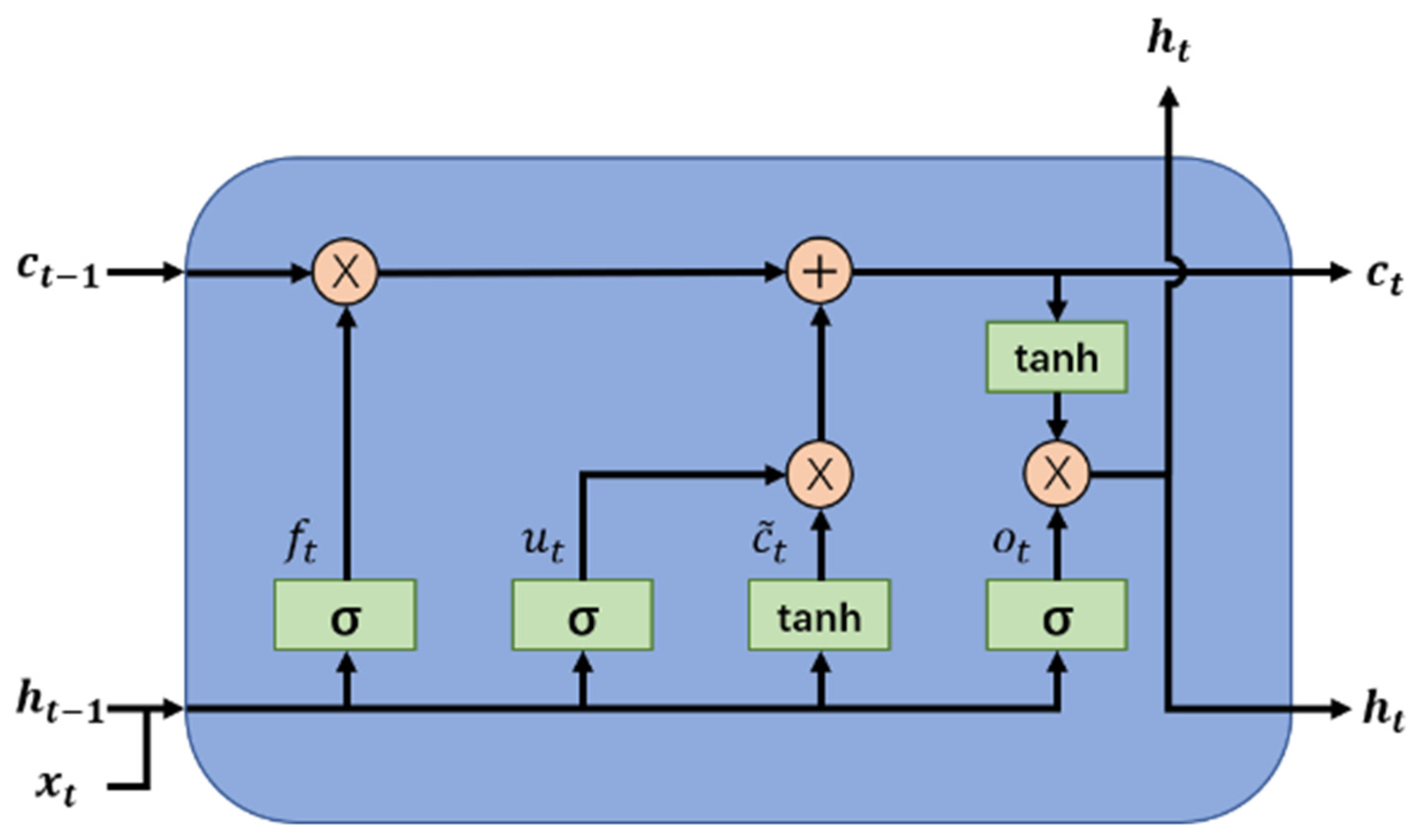
Figure 1 shows the updated cell (ct) in the LSTM model. The notations in Figure 1 are explained by following equations.
where represents the previous hidden state and represents the current time step input. refer to the forget gate, update gate, and output gate, respectively. represents the candidate cell state used to update the cell state. is the current cell state, represents the previous cell state, and represents the current hidden state. are weighted matrices while are bias terms. All these parameters are trainable. represents the Hadamard product. is the sigmoid function, and is the TanHyperbolic function. The two non-linear functions are defined in the following equations (more details related to LSTM can be found in [42]).
3.2. Graph Convolutional Network (GCN)
GCN is introduced to process graph-structured data, for example, a social network connection, road/public traffic network, etc. [43]. Graph structures consist of vertices and edges. We can abstract the passenger flows among bike-sharing stations into a graph to demonstrate the relationship among stations. In our study, stations are defined as vertices, and dependencies among stations are defined as edges. Therefore, a graph structure is constructed to demonstrate the passenger flows among stations.
Defining a graph, , where represents a set of vertices seized ; is a vector for every vertex, which contains one or more attributes about the vertex; represents a set of edges; and represents the adjacency matrix, where records the connection between the vertices.
We can define a computational efficiency formula to calculate the graph convolution:
where represents a diagonal degree matrix, with ; ; and the adjacency matrix does not contain the connection of the vertex itself. Therefore, the identity matrix will be summed to the adjacency matrix, ; . More details about deriving the graph convolution can be found in Xu et al. [44].
Generalizing the convolution calculation on the whole graph is represented with the symbol , where vertex has a feature vector and length of .
where is a parameter kernel that will be trained during the training process, is the convolved kernel, and is the number of hidden units in the neural network.
The adjacency matrix needs to be predefined before the training. Different predefinitions of adjacency will produce different results. The adjacency matrix can only contain 1 and 0 and is used to define the global adjacency relationship when it is predefined manually. In this case, it cannot well demonstrate the time-varied relations among the stations. To extract more precise relations, we use another learnable parameter to replace . This makes it easier to build a model than the adjacency matrix and improves the performance of the model. This replacement has been proved to be effective by Lin et al. [3]. The equation after the parameter replacement of Equation (10) is given as follows:
where is the learnable adjacency matrix. It is a symmetric matrix that consists of trainable kernel parameters, .
3.3. Attention Mechanism
Attention mechanism has been applied in many types of deep learning tasks and has shown good performance; for example, in image recognition, natural language processing, and voice recognition [45]. Basically, the attention function is pairing a query and multiple key-value pairs, and outputs a weighted sum of the values. The shape of the output varies depending on the level of the information you want to focus on, spatial information, temporal information, or any other parts. There are two kinds of attention mechanisms used in this paper. One is a temporal attention mechanism, and the other is a graph attention mechanism.
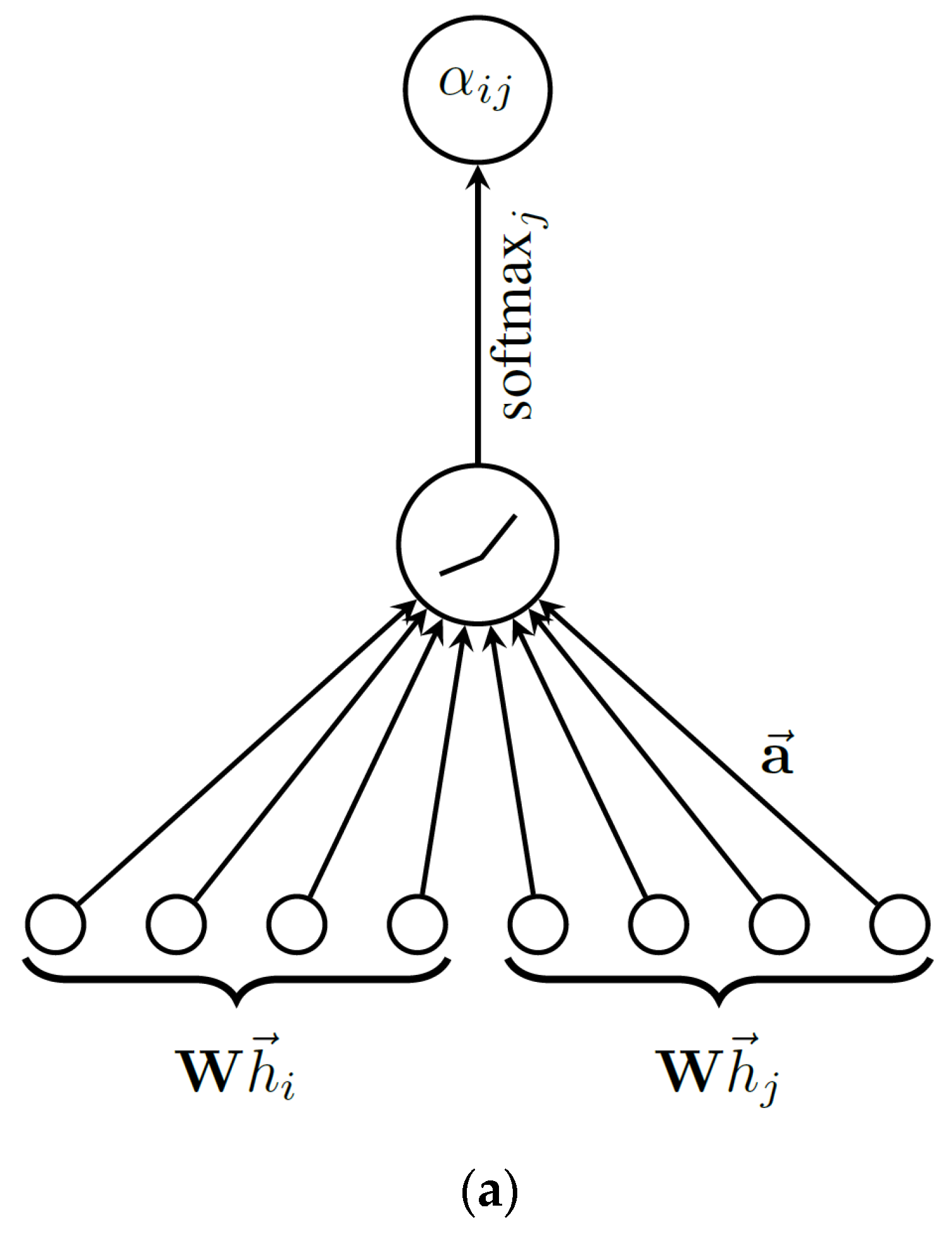
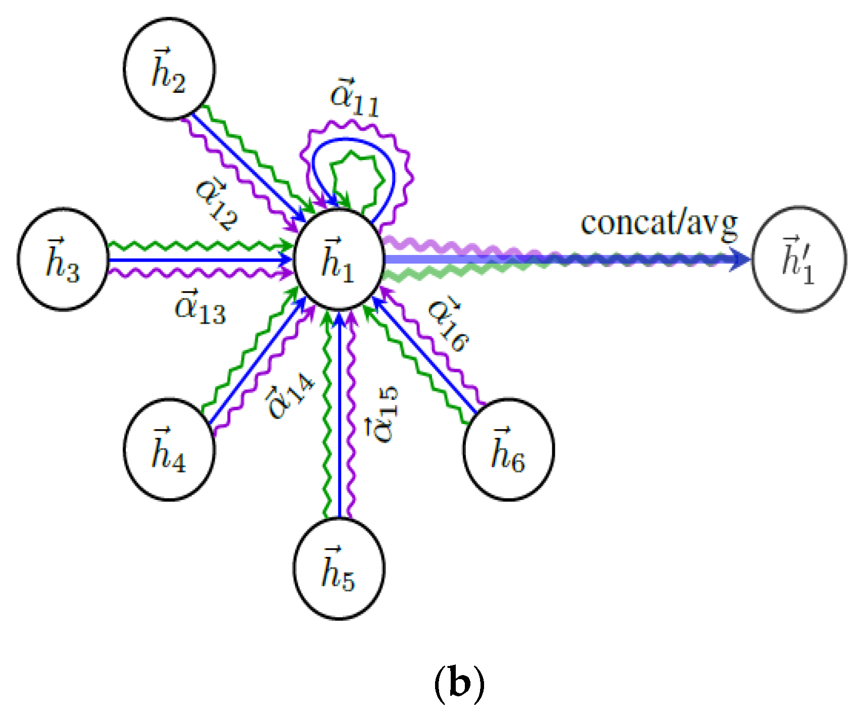
The graph attention mechanism is shown in Figure 2. Specifically, Figure 2a shows the feature transformation of vertices and gets the attention score. The features of the vertex itself, its neighbor vertices, and exogenous features are all transformed into the score. Figure 2b shows the multi-head attention method with a vertex on its neighborhood. The features aggregated from its neighbor vertices and itself are concatenated or averaged to obtain the attention vector.
The formulas of our attention mechanism are defined as follows:
where represents all neighborhood vertices of vertex is a weight matrix used for features transformation, signal represents the concatenation of vectors, is the weight of vertex calculated with function , represent the features of vertices , and refers to sigmoid function. The is defined as
where is a constant in .
After the attention scores are obtained, the attention enhanced hidden state can be represented as and be fed into the next GC-LSTM unit. The final output of each unit is shown as follows:
where is the spatial self-attention score tensor and is the current hidden state.
The temporal attention mechanism is a simplified graph attention mechanism; it only calculates the attention scores of the LSTM output sequence and gives the prediction with attention scores.
3.4. Spatial-Temporal Graph Attentional Long Short-Term Memory (STGA-LSTM)
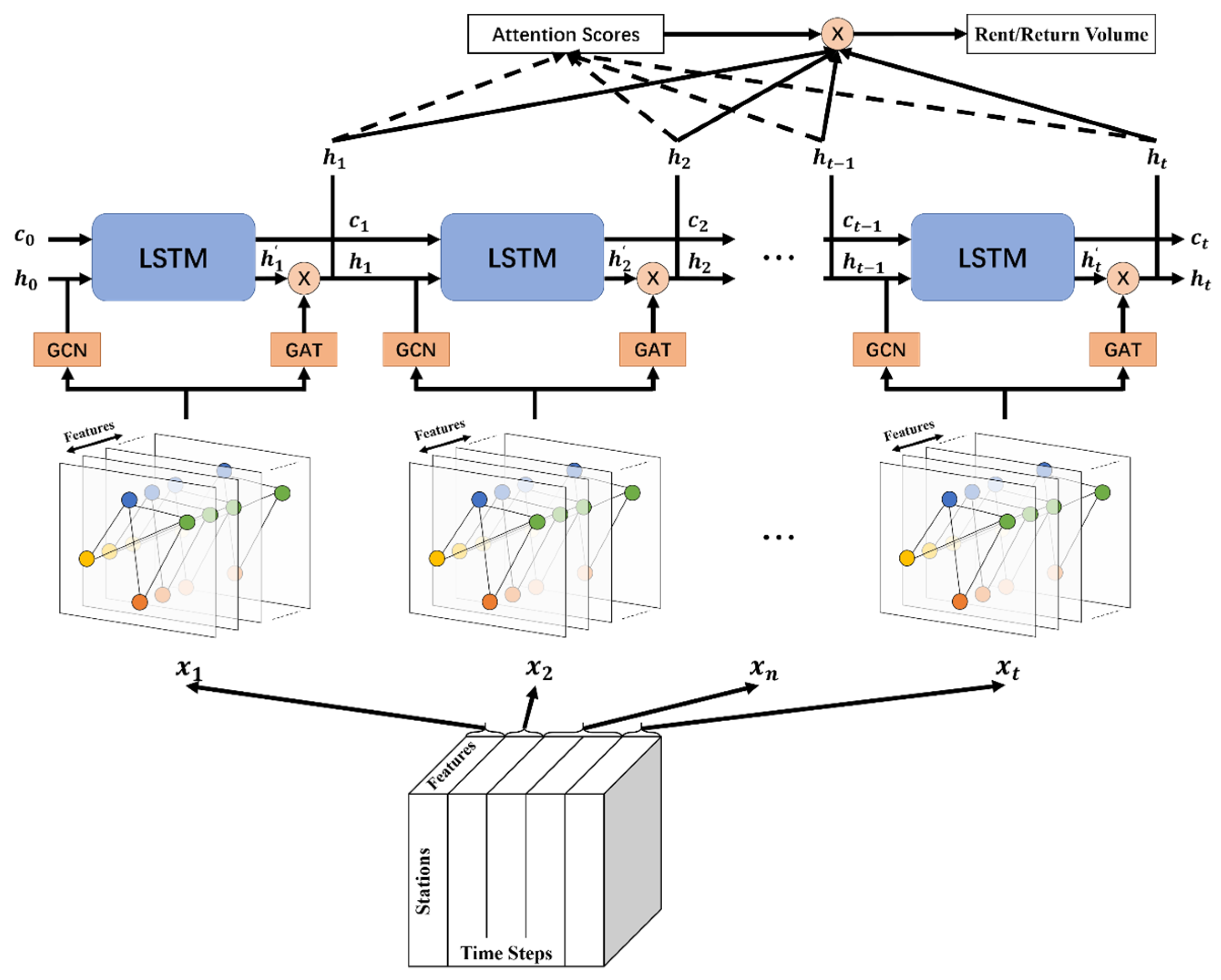
The three network components, namely, LSTM, GCN, and graph attention mechanism, are combined to establish the proposed neural network model structure STGA-LSTM.
The input data structure is a three-dimensional tensor that contains the features of each node at each time step. The exogenous variables can be concatenated at the dimension of features to demonstrate the information for each station.
Suppose the STGA-LSTM model contains several layers from input to output. Every vertex in the graph at layer has a feature vector with a length of , where . For each layer , the STGA-LSTM model propagates as follows:
where is the vector of the hidden state after implementing the temporal attention mechanism; , represents the convolved kernel at the layer; represents a weight parameter matrix for the layer; and is an activation function. In this paper, Rectified Linear Activation Unit (ReLU) is applied as the activation function, as shown in the following Formula (17). The ReLU function will retain a positive value and convert a negative value into zero; it allows faster and effective training of deep neural network architectures on large datasets [47]. is the output of the layer and the input of the layer, and , is the number of time steps.
The product of and can be replaced by one matrix during the training process. Therefore, Equation (16) can be simplified as follows:
where is the weight parameter matrix to be learned, and is the prediction sequence; e.g., the prediction of rental and return demand of the shared bikes in stations for the next hour. Figure 3 shows the whole process from input to output of the STGA-LSTM model. It visualizes the details of the connections between the different modules in the model. After the calculation by the input and hidden layer, the sequence is generated. It mines features from the input data. Then the sequence is fed into the output layer to obtain the final prediction; the last element in the sequence will be regarded as the final prediction in general. The output is the rental and return demand at each bike-sharing station. This proposed model auto-learns the spatial and temporal information among stations due to the combination of the graph convolution and LSTM structure.
4. Experiment
In this section, we compare several baseline models with our proposed STGA-LSTM model by using the bike-sharing dataset. First, the dataset and the data preprocessing are described. Second, the experimental settings, results, and discussion are described, and the effect of the exogenous variables on the prediction precision is explored. Then, the temporal and spatial scores at different prediction horizons are discussed.
4.1. Dataset Description
Data from multiple sources were obtained to predict the short-run bike-sharing demand. Nanjing Public Bicycle Company provided the bike-sharing trip dataset. The dataset involves 43,211 shared bikes and includes 3,230,204 bike-sharing transactions within the period of 1 September–30 September 2017. Each transaction records the rental station and time, return station and time, user ID, bike ID and, user personal information (gender, age, and birth place). The personal information is aggregated into stations at each prediction horizon.
Land-use data contain the POI number and road density within a radius of 300 m of each bike-sharing station [48]. POIs are obtained by calling the Amap API and are categorized into four groups, including working POIs, residential POIs, transport POIs, and other POIs [49]. The road shapefiles were obtained from OpenStreetMap [16] and the road density obtained by using ArcGIS.
4.2. Data Pre-Processing
This study focuses on the weekday period because the weekday demand for shared bikes is much heavier than weekend demand, and the bike-sharing rebalancing problem on weekdays is more serious than that on weekends. The bike-sharing transactions generated during weekdays were used to train the proposed model and test the performance. The dataset involved 21 weekdays. Data in the first 12 days were taken as the training dataset, the next 4 days were taken as the validation dataset, and the last 5 days were used as the testing dataset.
The origin dataset was processed into a matrix format, which contains the rental and return demand at each station. Then, the time-series data were generated based on the demand matrix in different prediction horizons, which can be fed into LSTM-based neuronal network models. represents bike-sharing demands of all stations at prediction horizon . Then, the time-series data were constructed with the demand from the previous time steps, , . The target vector is the bike-sharing demand at the next prediction horizon, . Therefore, the input data structure could be , where is the max time step at different prediction horizons. Ke et al. [51] showed that the demand information in recent time steps can help us build good models and yield satisfactory performance. Almannaa et al. [9] used 120-min data before the target prediction time to help prediction task. Therefore, the demand information in the previous two hours was used for predicting the demand at the next time step. The length of depends on the prediction horizon. For example, if the prediction horizon is 15 min, the length of is . We used the min and max normalization to scale the historical bike-sharing demand data between 0 and 1. The equation is shown as follows:
The land-use data, hourly weather data and personal information data were also normalized to (0, 1) based on Equation (19).
This study also considers the periodicity as an important attribute in historical bike-sharing demand. There were two differences made to the demand series data, namely, the first order difference and the seasonal difference. The step of the first order difference is 1 and the step of the seasonal difference was calculated based on the prediction horizon. The first order difference was used to eliminate the trend in the time-series data and seasonal difference was used to eliminate the time-series periodicity. The periodicity of bike-sharing demand was 1 day; therefore, the step of the seasonal difference was prediction horizon.
4.3. Experimental Setting
The following section lists the baseline models that we compared with the proposed model:
- (1)
- HA: Historical average prediction method. Using the average demand at the given location of the same related prediction horizon (i.e., the same time of the day) as the prediction value;
- (2)
- SVR: The radial basis function kernel-based Support Vector Regression (SVR). Fitting the curves by mapping the feature vectors into a high-dimension space. The cross validation is used to learn the kernel function and hyper parameters;
- (3)
- XGBoost: An implementation of Gradient Boosting Decision Trees (XGBoost), which is a scalable end-to-end tree boosting system. Compared with other tree boosting system, it uses fewer resources to scale beyond billions of datasets;
- (4)
- ANN: An artificial neural network that has two hidden layers. The hidden layers have the same number of dimensions as that of bike-sharing stations.
- (5)
- GCN: The number of dimensions of hidden layers and output layer is same as the ANN setting. The number of vertices in the graph equals that of bike-sharing stations.
- (6)
- LSTM: The number of dimensions of the hidden layers and output layer is same as the ANN setting. The number of LSTM units equals the number of time steps in different prediction horizon.
- (7)
- GC-LSTM: A Long Short-Term Memory neural network combined with a graph convolution operator. The number of dimensions of the hidden layers and output layer is same as the ANN setting. The number of vertices in the graph is equal to the number of bike-sharing stations. The number of LSTM units equals that of time steps in different prediction horizon.
All these baseline models were implemented or imported from existing packages by using Python 3.7. The neural network models including the baseline models and proposed model were all implemented based on TensorFlow 2.1.0. All the neural network models have an input layer, hidden layer, and output layer. The configurations of the computer on which these baseline models were trained and tested are as follows: OS: Windows 10; CPU: (Intel(R) Core(TM) i7-8700 CPU @ 3.20 GHz); RAM: 16 GB; plus one NVIDIA RTX 2060 GPU with 6 GB memory.
Hyper-parameters: In machine learning, hyper-parameters are predefined before the training process. Grid search, which is a traditional hyper-parameter optimization method, was used to find the optimized hyper-parameters. Three hyper-parameters were found out by using grid search, which are the learning rate, batch size, and the number of hidden units. Based on empirical tuning, the learning rate increases from 0.001 and stops at 0.01, and the step is 0.001. The batch size and the number of hidden units increase from 32 and stop at 128, and the step is 32. Time step selection is defined in Section 4.2, whose length depends on the prediction horizon.
We also set the criterion for the early stop process to prevent overfitting: When the mean absolute error (MAE) on validation does not decline by more than 0.00001 for over 10 training epochs, the training process stops.
Evaluation metrics: Root Mean Square Error (RMSE) and Mean Absolute Error (MAE) were used to assess the performance of the baseline models and proposed model, as Du et al. [12] and Li et al. [19] used:
where represents the observed value, represents the predicted value, and represents the amounts of testing samples.
4.4. Experimental Results and Discussion
As shown in Table 1, the evaluation criteria among the different models were compared to predict the bike-sharing rental and return demand. The RMSE and MAE of each model at various prediction horizons are the average of 10 times the training results. The smaller the value of the MAE and RMSE, the better the performance of the model. ANN, XGBoost, and SVR have worse performance than the GCN- and LSTM-based neural networks in each prediction horizon, because these three models cannot capture the hidden temporal information and hidden spatial relationships among stations.
LSTM and GCN have better performance than those three models, because LSTM can capture the hidden temporal information from the data and GCN has good ability to capture spatial attributes among data, especially for graph structure data. Besides, the comparison between GCN and LSTM can tell that the influence of spatial information contributes more to prediction accuracy than temporal information at a large time granularity. At a small time granularity, LSTM have more temporal information to capture, which makes the LSTM performance better than GCN at this situation. Combining GCN and LSTM, GC-LSTM performs better than GCN and LSTM because it integrates the attribute of those two models. STGA-LSTM has the best performance in each prediction horizon and under all criteria, followed by GC-LSTM in all the prediction models. After adding the attention mechanism with GC-LSTM, STGA-LSTM enhances the ability of capturing temporal and spatial information. When comparing STGA-LSTM with GC-LSTM, among the four different prediction horizons, the largest improvement occurs in the 15-min interval, with an increase of 4.49% in RMSE and 6.43% in MAE for rental demand prediction and an increase of 4.49% in RMSE and 6.43% in MAE for return demand prediction, respectively. This is because, given the total amount of data, the shorter the prediction horizon is, the longer the length of time sequence demand data will be. It will contain more detail when having a longer sequence demand data, which can help to improve the performance. The results explain why the RMSE and MAE grow larger as the prediction horizon turns larger.
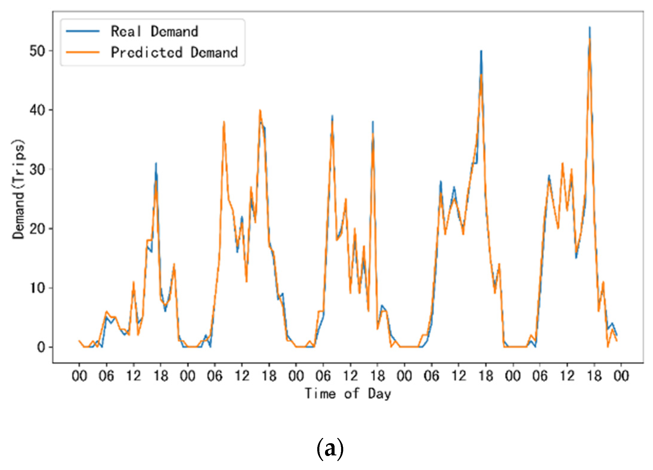
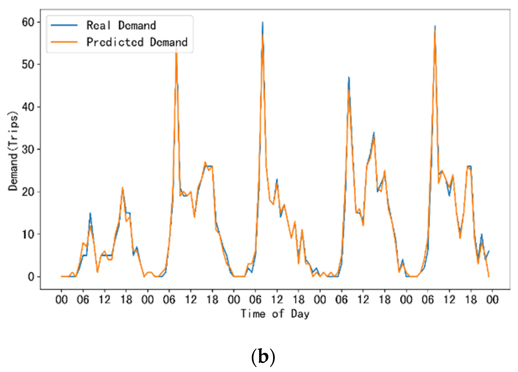
Figure 4 shows the comparison between the real demand curve and predicted demand curve in the 60-min prediction horizon at station No. 125. The datasets were drawn based on the training in the 60-min prediction horizon. This prediction horizon is a reasonable value for bike rebalancing [52]. We chose this station because it recorded the largest passenger flows among all stations, as the work in Pandya [33] did. The prediction is implemented by using the STGA-LSTM model with the test dataset. The test dataset has a time span of five days, consisting of 120 intervals. The predictions of rental demand and return demand are shown in Figure 4a and Figure 4b, respectively. We can see that both the rental and return demand prediction fit the real demand well, with very small offsets at the peak point. When predicting the peak demand, especially for those time that the demand suddenly raises up, the model loses some accuracy compared with the prediction accuracy in other periods. As for demand valleys, the proposed model performs well on both types of demand. In summary, the proposed STGA-LSTM model, as demonstrated in Figure 4, is able to produce reliable predictions on rental and return demand.
4.5. Efficiency Comparison
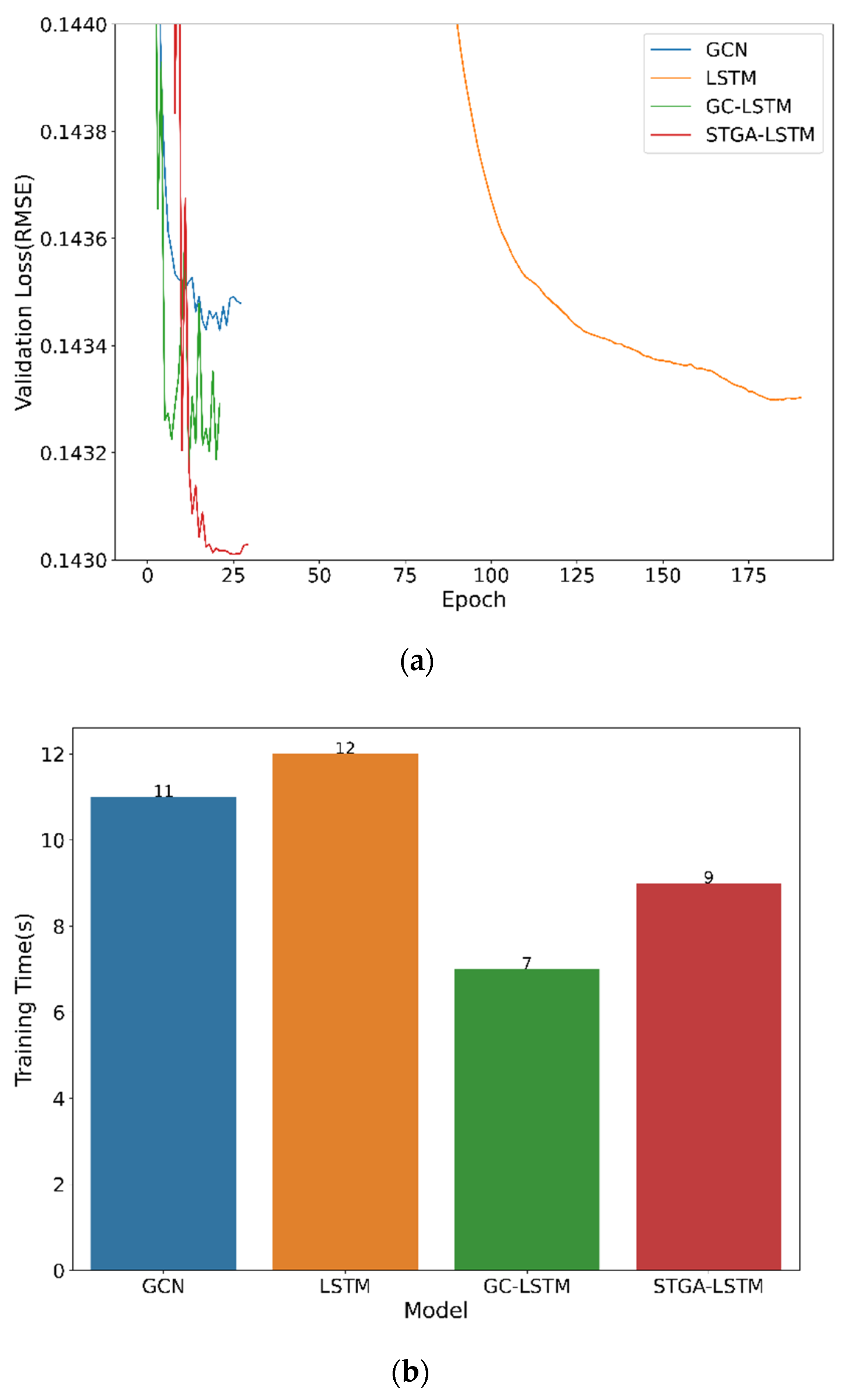
This section describes the training efficiency of the deep learning models, including GCN, and all the LSTM-based neural networks from the perspective of training epoch and training time. Figure 5a shows the validation loss along with training epoch and Figure 5b illustrates the total training time of each model. Figure 5 reflects the general pattern of how the validation loss changes during the training process and the time consumed for each model. LSTM performs the poorest among these four models. The convergence of the model is slow though it seems that it can be trained without overfitting with many training epochs. This may be because the maximum training epoch of 200 in this study makes the model unable to deliver its best possible performance. However, when the number of epochs increases, the time consumption will also be increased. The total training time consumed by GCN, GC-LSTM, and STGA-LSTM is similar, all around 10 s. These three models converge quickly at around 25 epochs. This shows that the three models learn pretty well on this dataset. However, GCN cannot extract the temporal information from the data, which makes it perform worse than GC-LSTM and STGA-LSTM on both the validation and test dataset. The total training time of GC-LSTM is shorter than the STGA-LSTM models because it does not use the attention mechanism to consider the hidden temporal information and spatial relationships among stations. STGA-LSTM converges faster than GC-LSTM, which proves the attention mechanism improves the model learning ability on the spatial information. The testing loss of STGA-LSTM is lower than GC-LSTM, which indicates that the attention mechanism helps the model find the hidden information from data and improve the accuracy.
4.6. Models with Exogenous Variables
The data of POIs, hourly weather, and personal information were included as the exogenous variables. The results are shown in Table 2. STGA-LSTM is used for testing the impact of the variables on the prediction accuracy in the 60-min interval. The inclusion of POIs, hourly weather, and personal information for the 60-min interval can slightly promote the prediction accuracy of the STGA-LSTMs in the 60-min interval. This is in line with the research of El-Assi et al. [53], which suggested that POIs and hourly weather contribute to the demand of docked shared bikes. We can see that the RMSE for the model with the full data is 0.8919, which has the best performance among all the models. Among all the exogenous factors, personal data contributes most to improve the prediction accuracy independently. This is reasonable because user groups are varying over time. For example, commuters are the main group who use shared bikes at the morning and afternoon peak for commuting purposes.
4.7. Temporal and Spatial Attention Mechanism
This section discusses the temporal and spatial attention scores at different prediction horizons.
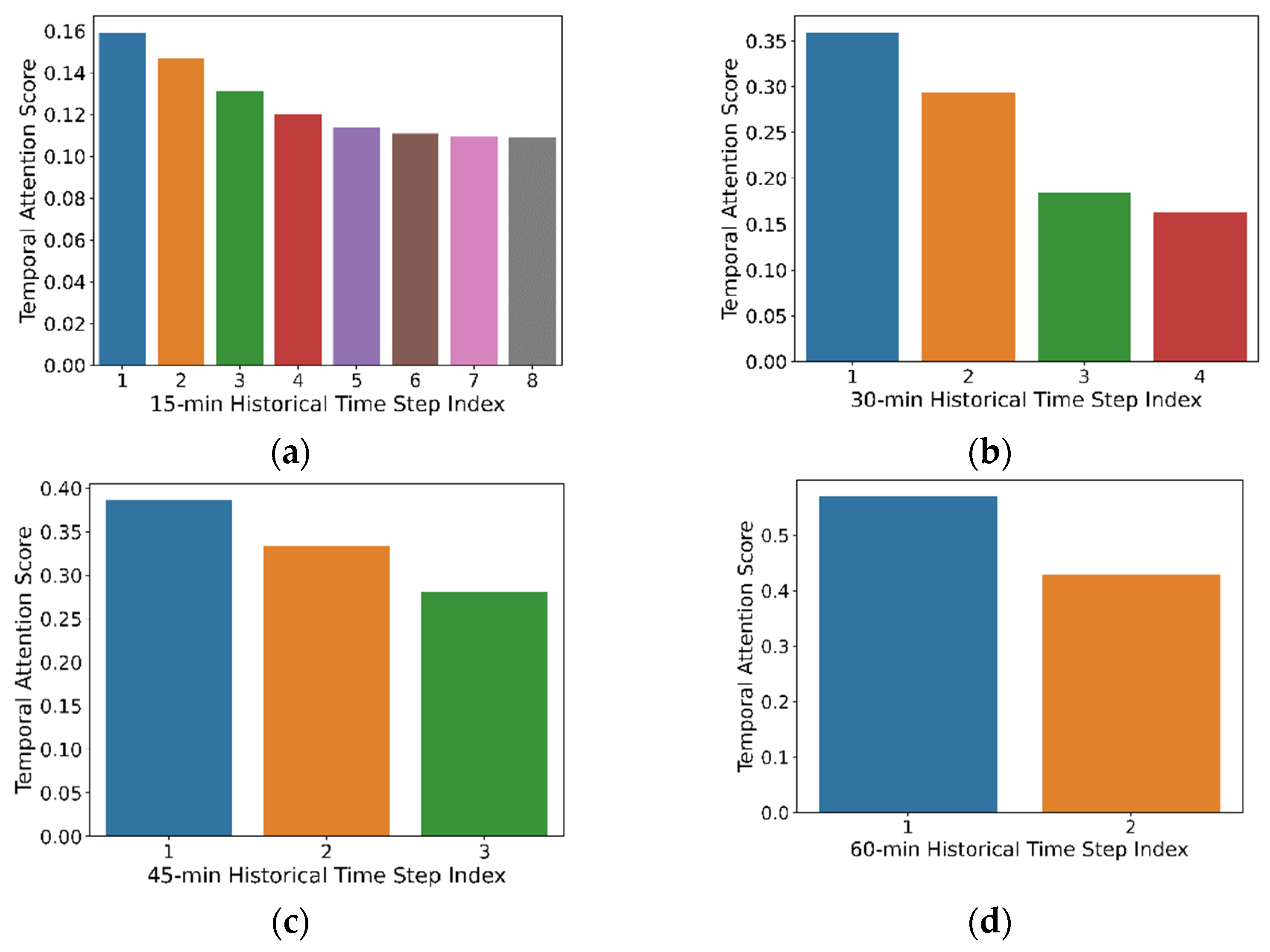
The temporal attention score for the prediction of shared-bike rental demand in the test dataset is visualized in Figure 6. Specially, Figure 6a–d represent the 15-min, 30-min, 45-min, and 60-min prediction horizon, respectively, and they all use two-hour history demand ahead of the target prediction time. The temporal attention mechanism can capture the important time-dimensional bike-sharing usage information. For example, the bike-sharing usage demand in the previous hour may have a certain influence on that in the next hour. The smaller time granularity can identify the time-dimensional bike-sharing usage information better and give a clearer overall picture. The historical time step index represents the time steps that the model looks back on from the historical time period. A smaller index means a closer time step to the prediction time. The temporal attention score represents the importance of bike-sharing usage demand in the corresponding time steps. The attention score will sum to 1 at different prediction horizons, respectively. For each prediction horizon, the temporal attention scores visualized in the figure is the average value of each time step from all the bike-sharing stations. From Figure 6a–d, all prediction horizons demonstrate that the closest historical data will always give the largest contribution to the prediction results. It is reasonable because the travel of bike-sharing will not last for a very long time; 90% bike-sharing travel takes less than 30 min [54]. It makes the usage of bike-sharing from the closest time period have the highest temporal correlation with the prediction period.
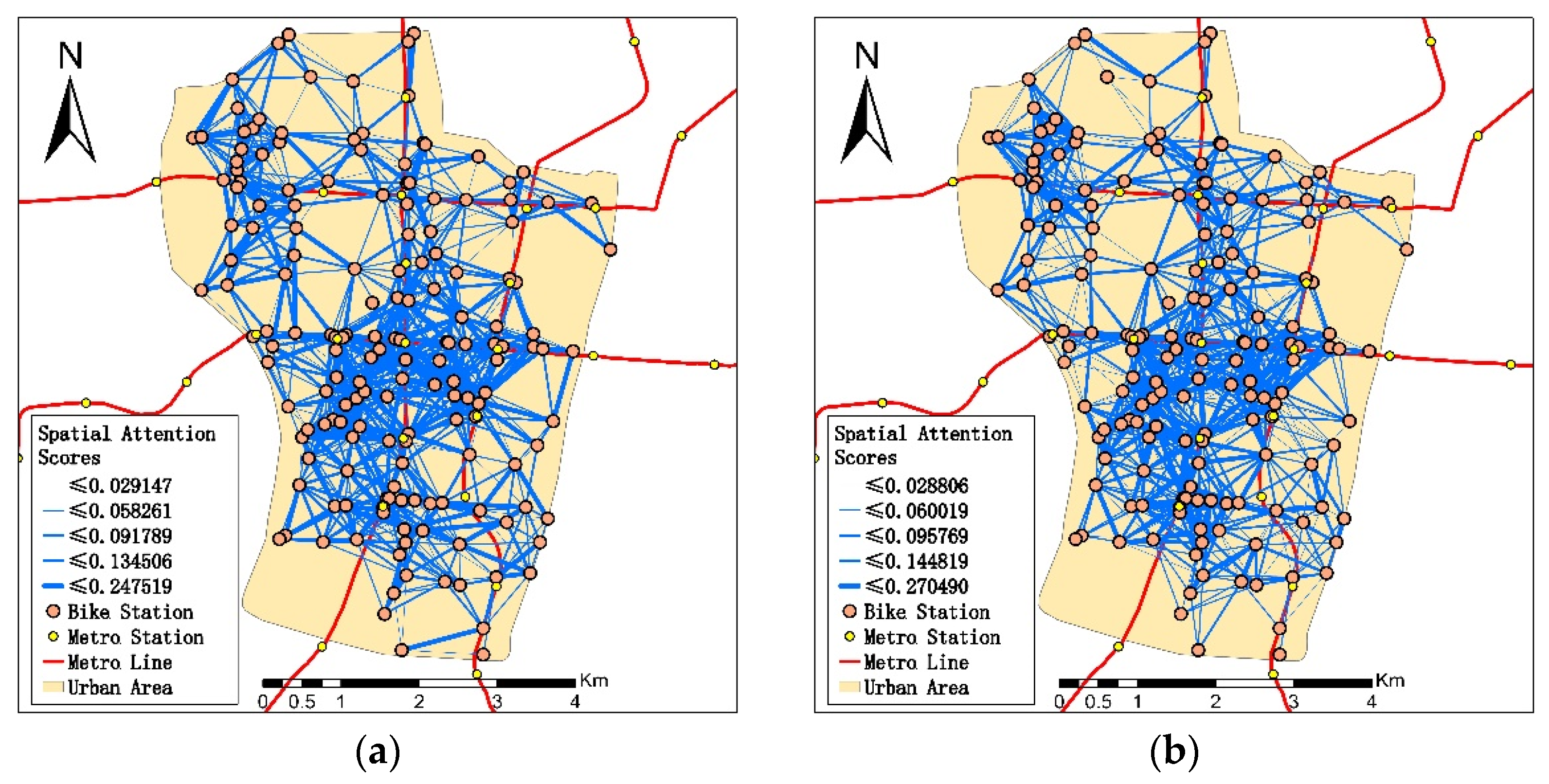
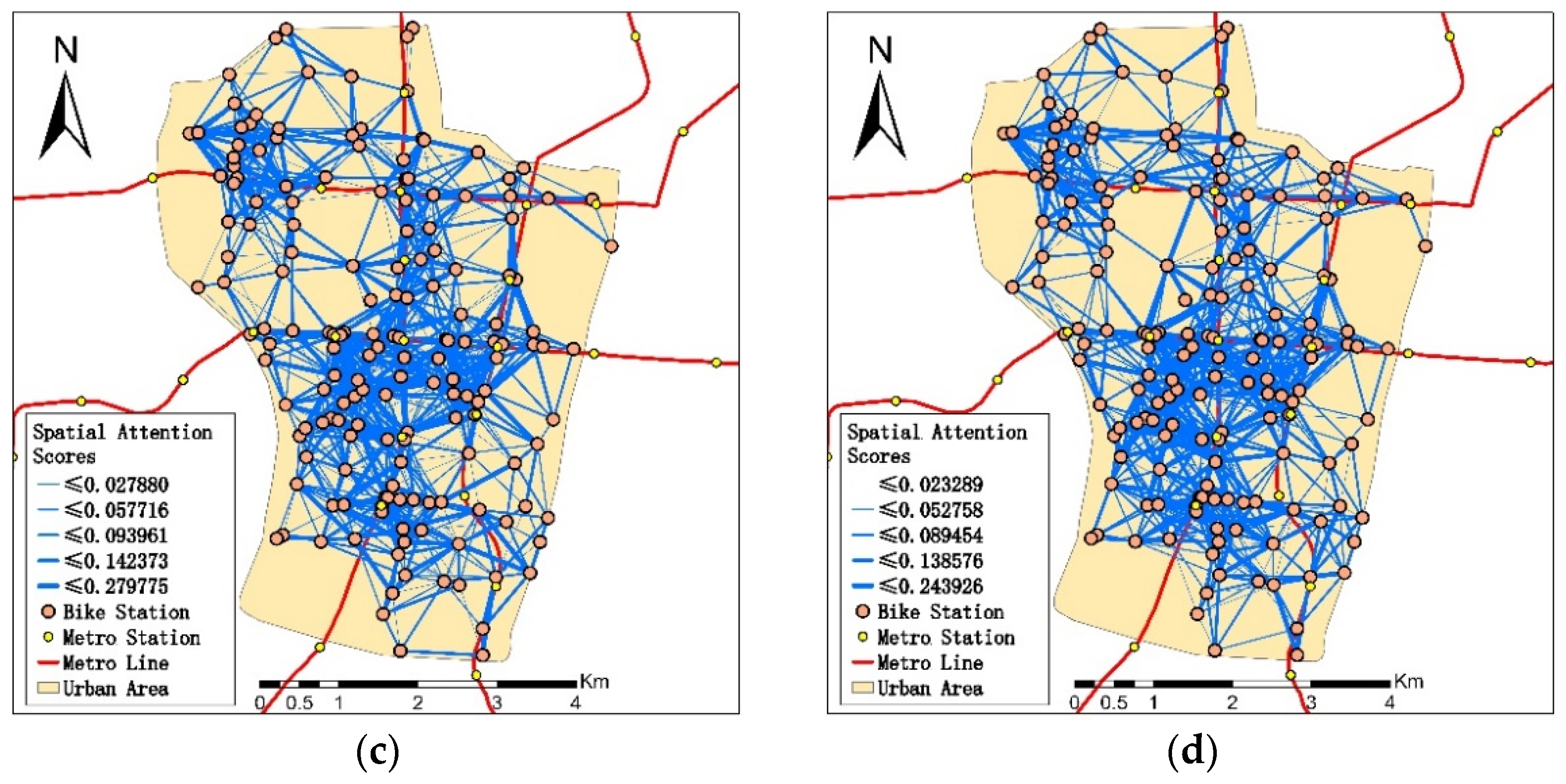
A visualization map of the spatial attention score can be found in Figure 7. Specially, Figure 7a–d represent the 15-min, 30-min, 45-min, and 60-min prediction horizon, respectively, and the line between the two stations represents the interaction between these two stations. The width of the blue line shows the value of the attention score among stations. The wider the line is, the stronger the interaction they have between two stations. The spatial attention mechanism could find the important space-dimensional bike-sharing usage information that can influence the usage demand of the bike-sharing stations. The bike-sharing usage demand is not only related to usage pattern of the rent/return bike-sharing stations, but also may be related to the stations around them. In Figure 7a–d, all the prediction horizons demonstrate that the density of the bike-sharing stations is an important factor that influences the correlation among stations. Stations always have a wider line connecting to those stations close to them, which means they have a stronger spatial connection to these stations. We can also see more connections among stations at a higher density area, and the usage of bike-sharing is higher in this area because of the convenience. When an area has a high density of bike-sharing stations, users can have multiple station choices when renting or returning the shared bikes. The walking distance among those stations is acceptable for users to switch from one station to another, which makes these stations more closely correlated [55]. When the high density of bike-sharing stations is low, the distance between the adjacent stations is large. It makes users more willing to travel by bus or metro instead of traveling by bike sharing [56]. The spatial weight among stations is not significantly influenced by time granularity, and a similar pattern can be found for different time granularities. Using a different time horizon from 15 to 60 min will not differentiate the spatial correlations.
5. Conclusions
This paper proposes an STGA-LSTM framework to predict the station-level short-term demand of a bike-sharing system by adopting multi-source data, including historical bike-sharing trip data, land-use data, weather data, and users’ personal information.
We used GCN to dig for spatial information and used LSTM to mine the temporal information from the data. The attention mechanism was applied to the spatio-temporal dimension simultaneously to deliver a more accurate prediction. We formulate the rental demand and return demand of shared bikes with a graph structure with our proposed STGA-LSTM model. The graph of the bike-sharing stations was constructed based on the demand connection among stations. In order to describe the relationship between stations and simplify the construction process, a learnable adjacency matrix was used in the model.
Experimental results of the real datasets obtained from the Nanjing bike-sharing systems validated that the proposed model is effective. The proposed model is more accurate and efficient than the baseline models, and exogenous variables can only slightly promote the prediction accuracy. Furthermore, we discuss the impact of the temporal and spatial attention mechanism. Temporal attention scores illustrate that, compared to other time steps, the closest historical time step influences the prediction result the most. Spatial attention scores indicate that a higher density of bike-sharing stations causes a stronger interaction among stations.
Further studies can be implemented from the following directions. First, the findings in this research are limited because the data used in this study only cover one-month docked bike-sharing data. Larger spatio-temporal datasets, such as metro passenger and dockless bike-sharing, can be used to conduct further investigations. Second, other types of external effects, such as metro passenger data and socioeconomic factors, should be considered to improve the prediction accuracy. In addition, the data for users’ personal characteristics can be limited, as indicated by previous research [57,58]. How to obtain the various and accurate personal data for research is worth investigating in future work. Finally, building a deeper network with our proposed model may promote accuracy, and maintaining a better balance between the cost of building a deeper network and the performance of the model should be considered during its implementation in the real world.
Author Contributions
The authors confirm their contributions to this paper as follows: X.M. and Y.J.: conceptualization, methodology, software; Y.Y., M.Z. and M.H.: investigation, writing—original draft preparation, writing—reviewing and editing. All authors checked the results and finalized the manuscript. All authors have read and agreed to the published version of the manuscript.
Funding
This research was funded by National Natural Science Foundation of China, grant number 52172304 and 51908187, and The APC was funded by National Natural Science Foundation of China, grant number 52172304.
Institutional Review Board Statement
Not applicable.
Informed Consent Statement
Not applicable.
Data Availability Statement
Not applicable.
Conflicts of Interest
The authors declare no conflict of interest.
References
- Yang, Z.; Chen, J.; Hu, J.; Shu, Y.; Cheng, P. Mobility Modeling and Data-Driven Closed-Loop Prediction in Bike-Sharing Systems. IEEE Trans. Intell. Transp. Syst. 2019, 20, 4488–4499. [Google Scholar] [CrossRef]
- Yang, M.; Liu, X.; Wang, W.; Li, Z.; Zhao, J. Empirical Analysis of a Mode Shift to Using Public Bicycles to Access the Suburban Metro: Survey of Nanjing, China. J. Urban Plan. Dev. 2016, 142, 05015011. [Google Scholar] [CrossRef]
- Lin, L.; He, Z.; Peeta, S. Predicting station-level hourly demand in a large-scale bike-sharing network: A graph convolutional neural network approach. Transp. Res. Part C Emerg. Technol. 2018, 97, 258–276. [Google Scholar] [CrossRef] [Green Version]
- The Meddin Bike-Sharing World Map. Available online: https://bikesharingworldmap.com/ (accessed on 23 April 2021).
- Gu, T.; Kim, I.; Currie, G. To be or not to be dockless: Empirical analysis of dockless bikeshare development in China. Transp. Res. Part A Policy Pract. 2019, 119, 122–147. [Google Scholar] [CrossRef]
- Pal, A.; Zhang, Y. Free-floating bike sharing: Solving real-life large-scale static rebalancing problems. Transp. Res. Part C Emerg. Technol. 2017, 80, 92–116. [Google Scholar] [CrossRef]
- Lazarus, J.; Pourquier, J.C.; Feng, F.; Hammel, H.; Shaheen, S. Micromobility evolution and expansion: Understanding how docked and dockless bikesharing models complement and compete—A case study of San Francisco. J. Transp. Geogr. 2020, 84, 102620. [Google Scholar] [CrossRef]
- Szeto, W.; Shui, C. Exact loading and unloading strategies for the static multi-vehicle bike repositioning problem. Transp. Res. Part B Methodol. 2018, 109, 176–211. [Google Scholar] [CrossRef]
- Almannaa, M.H.; Elhenawy, M.; Rakha, H.A. Dynamic linear models to predict bike availability in a bike sharing system. Int. J. Sustain. Transp. 2020, 14, 232–242. [Google Scholar] [CrossRef]
- Yang, H.; Xie, K.; Ozbay, K.; Ma, Y.; Wang, Z. Use of Deep Learning to Predict Daily Usage of Bike Sharing Systems. Transp. Res. Rec. J. Transp. Res. Board 2018, 2672, 92–102. [Google Scholar] [CrossRef]
- Chen, L.; Zhang, D.; Wang, L.; Yang, D.; Ma, X.; Li, S.; Wu, Z.; Pan, G.; Nguyen, T.M.T.; Jakubowicz, J. Dynamic cluster-based over-demand prediction in bike sharing systems. In Proceedings of the 2016 ACM International Joint Conference on Pervasive and Ubiquitous Computing, Heidelberg, Germany, 12–16 September 2016; pp. 841–852. [Google Scholar]
- Du, B.; Peng, H.; Wang, S.; Alam Bhuiyan, Z.; Wang, L.; Gong, Q.; Liu, L.; Li, J. Deep Irregular Convolutional Residual LSTM for Urban Traffic Passenger Flows Prediction. IEEE Trans. Intell. Transp. Syst. 2020, 21, 972–985. [Google Scholar] [CrossRef]
- Lin, F.; Jiang, J.; Fan, J.; Wang, S. A stacking model for variation prediction of public bicycle traffic flow. Intell. Data Anal. 2018, 22, 911–933. [Google Scholar] [CrossRef]
- Do, L.N.; Vu, H.L.; Vo, B.Q.; Liu, Z.; Phung, D. An effective spatial-temporal attention based neural network for traffic flow prediction. Transp. Res. Part C Emerg. Technol. 2019, 108, 12–28. [Google Scholar] [CrossRef]
- Amap. Available online: https://lbs.amap.com (accessed on 27 June 2020).
- OpenStreetMap. Available online: https://www.openstreetmap.org (accessed on 13 July 2020).
- Weather Underground. TWC Product and Technology LLC. Available online: https://www.wunderground.com/ (accessed on 20 July 2020).
- Sohrabi, S.; Paleti, R.; Balan, L.; Cetin, M. Real-time prediction of public bike sharing system demand using generalized extreme value count model. Transp. Res. Part A Policy Pr. 2020, 133, 325–336. [Google Scholar] [CrossRef]
- Li, Y.; Zhu, Z.; Kong, D.; Xu, M.; Zhao, Y. Learning Heterogeneous Spatial-Temporal Representation for Bike-Sharing Demand Prediction. In Proceedings of the AAAI Conference on Artificial Intelligence; Association for the Advancement of Artificial Intelligence (AAAI), Honolulu, HI, USA, 27 January–1 February 2019; Volume 33, pp. 1004–1011. [Google Scholar]
- Kaltenbrunner, A.; Meza, R.; Grivolla, J.; Codina, J.; Banchs, R. Urban cycles and mobility patterns: Exploring and predicting trends in a bicycle-based public transport system. Pervasive Mob. Comput. 2010, 6, 455–466. [Google Scholar] [CrossRef]
- Yoon, J.W.; Pinelli, F.; Calabrese, F. Cityride: A predictive bike sharing journey advisor. In Proceedings of the 2012 IEEE 13th International Conference on Mobile Data Management, Bengaluru, India, 2–26 July 2012; pp. 306–311. [Google Scholar]
- Gallop, C.; Tse, C.; Zhao, J. A Seasonal Autoregressive Model of Vancouver Bicycle Traffic Using Weather Variables. i-Manager’s J. Civ. Eng. 2011, 1, 9–18. [Google Scholar] [CrossRef]
- Wang, W. Forecasting Bike Rental Demand Using New York Citi Bike Data. Master’s Thesis, Dublin Institute of Technology, Dublin, Ireland, 2016. [Google Scholar]
- Froehlich, J.E.; Neumann, J.; Oliver, N. Sensing and predicting the pulse of the city through shared bicycling. In Proceedings of the Twenty-First International Joint Conference on Artificial Intelligence, Los Angeles, CA, USA, 12–17 July 2009; pp. 1420–1426. [Google Scholar]
- Hulot, P.; Aloise, D.; Jena, S.D. Towards station-level demand prediction for effective rebalancing in bike-sharing systems. In Proceedings of the 24th ACM SIGKDD International Conference on Knowledge Discovery & Data Mining, London, UK, 19–23 August 2018; pp. 378–386. [Google Scholar]
- Liu, J.; Li, Q.; Qu, M.; Chen, W.; Yang, J.; Xiong, H.; Zhong, H.; Fu, Y. Station site optimization in bike sharing systems. In Proceedings of the 2015 IEEE International Conference on Data Mining, Atlantic City, NJ, USA, 14–17 November 2015; pp. 883–888. [Google Scholar]
- Wang, B.; Kim, I. Short-term prediction for bike-sharing service using machine learning. Transp. Res. Procedia 2018, 34, 171–178. [Google Scholar] [CrossRef]
- Chen, P.; Hsieh, H.; Su, K.; Sigalingging, X.K.; Chen, Y.; Leu, J. Predicting station level demand in a bike-sharing system using recurrent neural networks. IET Intell. Transp. Syst. 2020, 14, 554–561. [Google Scholar] [CrossRef]
- Zhang, C.; Zhang, L.; Liu, Y.; Yang, X. Short-term prediction of bike-sharing usage considering public transport: A LSTM approach. In Proceedings of the 2018 21st International Conference on Intelligent Transportation Systems (ITSC), Maui, HI, USA, 4–7 November 2018; pp. 1564–1571. [Google Scholar]
- Ai, Y.; Li, Z.; Gan, M.; Zhang, Y.; Yu, D.; Chen, W.; Ju, Y. A deep learning approach on short-term spatiotemporal distribution forecasting of dockless bike-sharing system. Neural Comput. Appl. 2019, 31, 1665–1677. [Google Scholar] [CrossRef]
- Xu, M.; Liu, H.; Yang, H. A Deep Learning Based Multi-Block Hybrid Model for Bike-Sharing Supply-Demand Prediction. IEEE Access 2020, 8, 85826–85838. [Google Scholar] [CrossRef]
- Kim, T.S.; Lee, W.K.; Sohn, S.Y. Graph convolutional network approach applied to predict hourly bike-sharing demands considering spatial, temporal, and global effects. PLoS ONE 2019, 14, e0220782. [Google Scholar] [CrossRef]
- Pandya, D.A. Station-Graph: Bike Flow Prediction Using Spatio-Temporal Graph Convolutional Network. Master’s Thesis, California State University, California, CA, USA, 2020. [Google Scholar]
- Guo, R.; Jiang, Z.; Huang, J.; Tao, J.; Wang, C.; Li, J.; Chen, L. BikeNet: Accurate Bike Demand Prediction Using Graph Neural Networks for Station Rebalancing. In Proceedings of the 2019 IEEE Smart World, Ubiquitous Intelligence & Computing, Advanced & Trusted Computing, Scalable Computing & Communications, Cloud & Big Data Computing, Internet of People and Smart City Innovation (SmartWorld/SCALCOM/UIC/ATC/CBDCom/IOP/SCI), Leicester, UK, 19–23 August 2019; pp. 686–693. [Google Scholar]
- Yoshida, A.; Yatsushiro, Y.; Hata, N.; Higurashi, T.; Tateiwa, N.; Wakamatsu, T.; Tanaka, A.; Nagamatsu, K.; Fujisawa, K. Practical End-to-End Repositioning Algorithm for Managing Bike-Sharing System. In Proceedings of the 2019 IEEE International Conference on Big Data (Big Data), Los Angeles, CA, USA, 9–12 December 2019; pp. 1251–1258. [Google Scholar]
- Chai, D.; Wang, L.; Yang, Q. Bike flow prediction with multi-graph convolutional networks. In Proceedings of the 26th ACM SIGSPATIAL International Conference on Advances in Geographic Information Systems, Washington, DC, USA, 6–9 November 2018; pp. 397–400. [Google Scholar]
- Zhou, X.; Shen, Y.; Zhu, Y.; Huang, L. Predicting multi-step citywide passenger demands using attention-based neural networks. In Proceedings of the Eleventh ACM International Conference on Web Search and Data Mining, Los Angeles, CA, USA, 5–9 February 2018; pp. 736–744. [Google Scholar]
- Useche, S.A.; Esteban, C.; Alonso, F.; Montoro, L. Are Latin American cycling commuters “at risk”? A comparative study on cycling patterns, behaviors, and crashes with non-commuter cyclists. Accid. Anal. Prev. 2021, 150, 105915. [Google Scholar] [CrossRef] [PubMed]
- Lock, O. Cycling Behaviour Changes as a Result of COVID-19: A Survey of Users in Sydney, Australia. Transp. Find. 2020, 13405. [Google Scholar] [CrossRef]
- Li, X.; Useche, S.A.; Zhang, Y.; Wang, Y.; Oviedo-Trespalacios, O.; Haworth, N. Comparing the cycling behaviours of Australian, Chinese and Colombian cyclists using a behavioural questionnaire paradigm. Accid. Anal. Prev. 2021, 164, 106471. [Google Scholar] [CrossRef] [PubMed]
- Bengio, Y.; Simard, P.; Frasconi, P. Learning long-term dependencies with gradient descent is difficult. IEEE Trans. Neural Netw. 1994, 5, 157–166. [Google Scholar] [CrossRef] [PubMed]
- Hochreiter, S.; Schmidhuber, J. Long short-term memory. Neural Comput. 1997, 9, 1735–1780. [Google Scholar] [CrossRef] [PubMed]
- Bruna, J.; Zaremba, W.; Szlam, A.; LeCun, Y. Spectral networks and locally connected networks on graphs. arXiv 2013, arXiv:1312.6203. [Google Scholar]
- Xu, K.; Hu, W.; Leskovec, J.; Jegelka, S. How powerful are graph neural networks? arXiv 2018, arXiv:1810.00826. [Google Scholar]
- Luo, Y.; Liu, Q.; Zhu, H.; Fan, H.; Song, T.; Yu, C.W.; Du, B. Multistep Flow Prediction on Car-Sharing Systems: A Multi-Graph Convolutional Neural Network with Attention Mechanism. Int. J. Softw. Eng. Knowl. Eng. 2019, 29, 1727–1740. [Google Scholar]
- Veličković, P.; Cucurull, G.; Casanova, A.; Romero, A.; Liò, P.; Bengio, Y. Graph Attention Networks. arXiv 2017, arXiv:1710.10903. [Google Scholar]
- Krizhevsky, A.; Sutskeve, I.; Hinton, G.E. Imagenet classification with deep convolutional neural networks. Adv. Neural Inf. Process. Syst. 2017, 60, 84–90. [Google Scholar] [CrossRef]
- Zhao, D.; Ong, G.P.; Wang, W.; Hu, X.J. Effect of built environment on shared bicycle reallocation: A case study on Nanjing, China. Transp. Res. Part A Policy Pr. 2019, 128, 73–88. [Google Scholar] [CrossRef]
- Ji, Y.; Ma, X.; He, M.; Jin, Y.; Yuan, Y. Comparison of usage regularity and its determinants between docked and dockless bike-sharing systems: A case study in Nanjing, China. J. Clean. Prod. 2020, 255, 120110. [Google Scholar] [CrossRef]
- Xu, C.; Ji, J.; Liu, P. The station-free sharing bike demand forecasting with a deep learning approach and large-scale datasets. Transp. Res. Part C Emerg. Technol. 2018, 95, 47–60. [Google Scholar] [CrossRef]
- Ke, J.; Zheng, H.; Yang, H.; Chen, X.M. Short-term forecasting of passenger demand under on-demand ride services: A spatio-temporal deep learning approach. Transp. Res. Part C Emerg. Technol. 2017, 85, 591–608. [Google Scholar] [CrossRef] [Green Version]
- Elhenawy, M.; Bichiou, Y.; Rakha, H. A heuristic algorithm for rebalancing large-scale bike sharing systems using multiple trucks. In Proceedings of the Transportation Research Board 98th Annual Meeting, Washington, DC, USA, 13–17 January 2019. [Google Scholar]
- El-Assi, W.; Mahmoud, M.S.; Habib, K.N. Effects of built environment and weather on bike sharing demand: A station level analysis of commercial bike sharing in Toronto. Transportation 2017, 44, 589–613. [Google Scholar] [CrossRef]
- Ma, X.; Yuan, Y.; Oort, N.; Ji, Y.; Hoogendoorn, S. Understanding the difference in travel patterns between docked and dockless bike-sharing systems: A case study in Nanjing, China. In Proceedings of the 98th Transportation Research Board Annual Meeting, Washington, DC, USA, 13–17 January 2019; pp. 13–17. [Google Scholar]
- Ma, X.; Zhang, J.; Ding, C.; Wang, Y. A geographically and temporally weighted regression model to explore the spatiotemporal influence of built environment on transit ridership. Comput. Environ. Urban Syst. 2018, 70, 113–124. [Google Scholar] [CrossRef]
- Li, J.; Guo, X.; Zhang, X.; Lv, F. Operation Characteristics of Free-Floating Bike Sharing System as a Feeder Mode to Rail Transit Based on GPS Data: A case study in Beijing. In Proceedings of the Transportation Research Board 98st Annual Meeting, Washington, DC, USA, 13–17 January 2019. [Google Scholar]
- Vidotto, G.; Anselmi, P.; Filipponi, L.; Tommasi, M.; Saggino, A. Using Overt and Covert Items in Self-Report Personality Tests: Susceptibility to Faking and Identifiability of Possible Fakers. Front. Psychol. 2018, 9, 1100. [Google Scholar] [CrossRef]
- Alonso, F.; Faus, M.; Esteban, C.; Useche, S. Is There a Predisposition towards the Use of New Technologies within the Traffic Field of Emerging Countries? The Case of the Dominican Republic. Electronics 2021, 10, 1208. [Google Scholar] [CrossRef]
Figure 1.
Structure of the LSTM unit.

Figure 2.
Graphic illustration of the attention mechanism [46]. (a) Extracting features from neighborhood vertices; (b) Multi-head attention method.
Figure 2.
Graphic illustration of the attention mechanism [46]. (a) Extracting features from neighborhood vertices; (b) Multi-head attention method.


Figure 3.
The whole process of the STGA-LSTM model.

Figure 4.
Performance of the rental and return demand prediction. (a) Real rental demand and predicted rental demand at station No. 125; (b) Real return demand and predicted return demand at station No. 125.
Figure 4.
Performance of the rental and return demand prediction. (a) Real rental demand and predicted rental demand at station No. 125; (b) Real return demand and predicted return demand at station No. 125.


Figure 5.
Model performance comparison of GCN and all the LSTM-based models. (a) Validation loss along with training epoch; (b) Total training time.
Figure 5.
Model performance comparison of GCN and all the LSTM-based models. (a) Validation loss along with training epoch; (b) Total training time.

Figure 6.
Temporal attention score for each time step of the different prediction horizons. (a) 15-min horizon; (b) 30-min horizon; (c) 45-min horizon; (d) 60-min horizon.
Figure 6.
Temporal attention score for each time step of the different prediction horizons. (a) 15-min horizon; (b) 30-min horizon; (c) 45-min horizon; (d) 60-min horizon.

Figure 7.
Spatial attention score among stations of the different prediction horizons. (a) 15-min horizon; (b) 30-min horizon; (c) 45-min horizon; (d) 60-min horizon.
Figure 7.
Spatial attention score among stations of the different prediction horizons. (a) 15-min horizon; (b) 30-min horizon; (c) 45-min horizon; (d) 60-min horizon.


Table 1.
Predictive performance of different models on the test dataset.
| Model | Rental Volume | Return Volume | Rental Volume | Rental Volume | ||||
|---|---|---|---|---|---|---|---|---|
| RMSE | MAE | RMSE | MAE | RMSE | MAE | RMSE | MAE | |
| 15 min | 45 min | |||||||
| HA | 1.2370 | 0.7269 | 1.2204 | 0.7194 | 2.5817 | 1.4848 | 2.5270 | 1.4594 |
| ANN | 0.8637 | 0.4951 | 0.8660 | 0.4976 | 0.9865 | 0.6190 | 1.1461 | 0.7451 |
| XGBoost | 0.8737 | 0.4953 | 0.8754 | 0.4986 | 1.0827 | 0.6738 | 1.0857 | 0.6803 |
| SVR | 0.9649 | 0.5635 | 0.9706 | 0.5663 | 1.1277 | 0.7307 | 0.9800 | 0.6106 |
| LSTM | 0.7139 | 0.3843 | 0.7397 | 0.4034 | 0.8513 | 0.5140 | 0.8509 | 0.5084 |
| GCN | 0.7600 | 0.4196 | 0.6815 | 0.3585 | 0.8477 | 0.5066 | 0.8475 | 0.5109 |
| GC-LSTM | 0.6415 | 0.3314 | 0.6735 | 0.3551 | 0.8410 | 0.5040 | 0.8452 | 0.5071 |
| STGA-LSTM | 0.6127 | 0.3101 | 0.6107 | 0.3088 | 0.7912 | 0.4663 | 0.7930 | 0.4690 |
| 30 min | 60 min | |||||||
| HA | 1.9530 | 1.1399 | 1.9087 | 1.1155 | 3.2052 | 1.8228 | 3.1310 | 1.7844 |
| ANN | 0.9450 | 0.5740 | 1.0903 | 0.6852 | 1.0845 | 0.6910 | 1.2304 | 0.8218 |
| XGBoost | 0.9848 | 0.5999 | 0.9917 | 0.6035 | 1.1825 | 0.7602 | 1.1700 | 0.7547 |
| SVR | 1.1041 | 0.6949 | 0.9454 | 0.5747 | 1.2613 | 0.8383 | 1.0775 | 0.6886 |
| LSTM | 0.7912 | 0.4573 | 0.8001 | 0.4651 | 0.9484 | 0.5839 | 0.9972 | 0.6218 |
| GCN | 0.8014 | 0.4651 | 0.7784 | 0.4480 | 1.0230 | 0.6414 | 0.9406 | 0.5834 |
| GC-LSTM | 0.7266 | 0.4078 | 0.7332 | 0.4134 | 0.9126 | 0.5527 | 0.9137 | 0.5586 |
| STGA-LSTM | 0.7098 | 0.3952 | 0.7118 | 0.3978 | 0.8979 | 0.5418 | 0.8998 | 0.5440 |
Table 2.
Predictive performance of the different exogenous variables.
| Variables | RMSE | MAE |
|---|---|---|
| STGA-LSTM (historical data only) | 0.8979 | 0.5418 |
| STGA-LSTM (POIs and road density data) | 0.8966 | 0.5407 |
| STGA-LSTM (hourly weather data) | 0.8969 | 0.5413 |
| STGA-LSTM (personal data) | 0.8956 | 0.5395 |
| STGA-LSTM (full data) | 0.8919 | 0.5415 |
Publisher’s Note: MDPI stays neutral with regard to jurisdictional claims in published maps and institutional affiliations. |
© 2022 by the authors. Licensee MDPI, Basel, Switzerland. This article is an open access article distributed under the terms and conditions of the Creative Commons Attribution (CC BY) license (https://creativecommons.org/licenses/by/4.0/).
Share and Cite
MDPI and ACS Style
Ma, X.; Yin, Y.; Jin, Y.; He, M.; Zhu, M. Short-Term Prediction of Bike-Sharing Demand Using Multi-Source Data: A Spatial-Temporal Graph Attentional LSTM Approach. Appl. Sci. 2022, 12, 1161. https://doi.org/10.3390/app12031161
AMA Style
Ma X, Yin Y, Jin Y, He M, Zhu M. Short-Term Prediction of Bike-Sharing Demand Using Multi-Source Data: A Spatial-Temporal Graph Attentional LSTM Approach. Applied Sciences. 2022; 12(3):1161. https://doi.org/10.3390/app12031161
Chicago/Turabian StyleMa, Xinwei, Yurui Yin, Yuchuan Jin, Mingjia He, and Minqing Zhu. 2022. "Short-Term Prediction of Bike-Sharing Demand Using Multi-Source Data: A Spatial-Temporal Graph Attentional LSTM Approach" Applied Sciences 12, no. 3: 1161. https://doi.org/10.3390/app12031161
Note that from the first issue of 2016, this journal uses article numbers instead of page numbers. See further details here.