Article

Modeling and Validation of a Passive Truss-Link Mechanism for Deployable Structures Considering Friction Compensation with Response Surface Methods

1
Department of Mechanical Engineering, Jeonbuk National University, 567 Baekje-daero, Deokjin-gu, Jeonju-si 54896, Jeollabuk-do, Korea
2
Hanwha System, 491-23, Gyeonggidong-ro, Namsa-eup, Cheoin-gu, Yongin-si 17121, Gyeonggi-do, Korea
3
SaTReC (Satellite Technology Research Center), KAIST, 291, Daehak-ro, Yuseong-gu, Daejeon 34141, Korea
*
Author to whom correspondence should be addressed.
Appl. Sci. 2022, 12(1), 451; https://doi.org/10.3390/app12010451
Submission received: 13 November 2021 / Revised: 30 December 2021 / Accepted: 1 January 2022 / Published: 4 January 2022

Abstract

:
In this study, a passive truss-link mechanism applicable to large-scale deployable structures was designed to achieve successful deployment in space. First, we simplified the selected truss-link mechanisms to the two-dimensional geometry and calculated the degrees of freedom (DOF) to determine whether a kinematic over-constraint occurs. The dimensions of the truss-link structure were determined through a deployment kinematic analysis. Second, a deployment simulation with the truss-link was conducted using multibody dynamics (MBD) software. Finally, a deployment test was performed considering gravity compensation, and the results were compared with those of MBD simulation. The results of the deployment simulations were confirmed to be slightly faster than those of the deployment test due to friction effects existing in the joints and gravity compensation devices. To address this issue, inverse identification of the equivalent frictional torque (EFT) at the revolute joints in the deployment test was conducted through response surface methods (RSM) combined with the central composite design technique. As a result, we confirmed that the deployment angle history of the deployment simulation was similar to that of the deployment test.

1. Introduction

Synthetic aperture radar (SAR), which can provide high-resolution earth images regardless of weather conditions or time of day has recently been used in various fields of domestic and international observation satellites [1,2]. In the case of SAR antennas, to maximize resolution and power gain in acquiring high-resolution images, a large deployable panel is accommodated. However, to deploy such a large space deployment structure in orbit, it is essential to use specific mechanisms that allow the structure to be appropriately folded and stored inside the launch-vehicle fairing and fully deployed in orbit [1,2,3,4,5,6].
Furthermore, when a satellite performs a mission, line-of-sight (LOS) pointing stability must be secured. During ground imaging, if the relatively large antenna is shaken by external or internal disturbances, the quality of the captured images will be degraded. Therefore, the stiffness of the rotational spring hinges of deployable panels is often increased in order to obtain high deployment stability. This mechanism shortens the deployment time but leads to a high impact load when fully deployed and latched. This deployment impact load could cause damage to structures, payloads, and solar cells. By contrast, decreased stiffness of the rotational spring hinges reduces the deployment impact load by increasing the deployment time, but cannot guarantee successful full deployment due to harness resistance and mechanical friction of deployment devices at low temperatures [7].
In response to these issues, a variety of methods have been proposed to allow stable deployment and reduce deployment impact loads, such as a torsion spring-latching hinge [8], tape spring hinge [9], and shape memory alloy (SMA)-based hinge [10]. However, these deployment mechanisms still have limitations including low deployment stiffness of the relatively large deployable structures. To address this, truss-link mechanisms [11] have been applied to many satellite missions to increase the deployment stiffness: ERS-1 [12], RADARSAT-1 [13], RADARSAT-2 [14], RADARSAT-Constellation [15], ALOS-2 [16], SEASAT [17], WorldView-4 [18], and Sentinel-5P [19]. Among these, the RADARSAT mission employed the truss-link mechanism to increase deployment stiffness and attempted to reduce the number of truss-links as the follow-up mission progressed to reduce weight. Comparing the number of truss-links in satellites, RADARSAT-1 (1995) has 30 links, RADARSAT-2 (2007) has 22 links, and RADARSAT-Constellation (2019) has four links. The reduction in the number of links is the result of a trend to build up small satellites for constellation missions. In addition, the applications of the truss-link mechanisms have been diversified. Wang et al. proposed a pyramid deployable truss structure (PDTS) design for deployable SAR antennas through an analytical approach based on weighted graphs and kinematic chain techniques [20]. They also proposed a modular deployable truss structure (MDTS) for large SAR antennas [13] with a scaled model. A difference was found between the deployment test and the simulation, however, due to uneven and indeterminate ground friction as well as joint friction. Furthermore, to eliminate interference during the deployment process of the truss structure, the optimal motor driving torque was determined through the design of experiments (DOE) method. Han et al. proposed a large-scale deployable ring truss that composes a space antenna by complementing a rope-based actuation and cable net system [21]. Based on the absolute node coordinate formulation (ANCF), a method for simulating the rigid body motion of the antenna support arm was proposed, and the friction and motion equations of the flexible cable net were presented using the Lagrange equation.
Most of the aforementioned works essentially assume that an active driving mechanism such as motors with cables is employed for large-scale SAR antenna structures. However, such an active mechanism is hardly employed for small satellites due to deployment costs and complexity. In addition, the friction effects cannot be neglected as they generate a difference between deployment tests and simulations.
The goal of this work is to propose a passive truss-link mechanism for large deployable structures of small satellites. In contrast to the many truss-link mechanisms [11,12,13,14,15,16,17], we do not accommodate any active driving mechanisms because they are not simple and not sufficiently reliable. As driving mechanisms, only conventional torsion spring hinges with proper latching mechanisms were employed in this work. To achieve successful deployment, an inverse identification technique for equivalent friction torque (EFT) was proposed based on the results of the response surface method combined with the central composite design technique. Finally, a torque margin analysis was conducted to predict whether the deployment would be successful.
This works consisted of three sections: first, we discussed the configuration design from conceptual design to detailed modeling considering deployment kinematics. Second, deployment dynamics simulations and tests were conducted. To minimize the discrepancy between the test and simulation, the friction-compensation technique was introduced, and results were verified by a torque margin analysis. Finally, we provided concluding remarks.

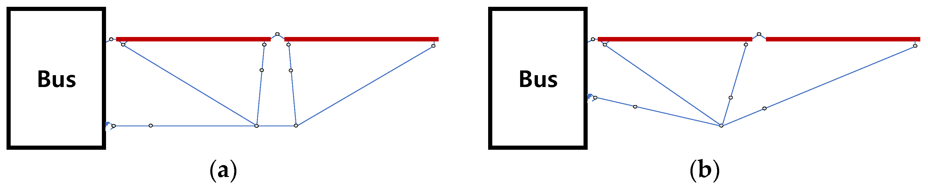
2. Configuration Design of Truss-Link Mechanism

2.1. Concept Design

For full deployment of deployable structures with truss-links, the total degrees of freedom (DOF) has to be checked to determine whether the structure is over-constrained. If the DOF of the deployable structure becomes negative, the deployment will fail due to over-constraint problems. First, we analyzed the DOF by referring to RADARSAT-1 and RADARSAT-2 satellites using truss-links [13,14]. Two-dimensional (2D) designs of one payload wing of the satellite were considered, Type 1 (RADARSAT-1) and Type 2 (RADARSAT-2), to analyze the DOF, as seen in Figure 1. We employed Gruebler’s equation, as shown in Equation (1) to evaluate the total DOF [22].
S y s D O F = 3 ( L 1 ) 2 J 1 J 2
Here, SysDOF represents the total DOF of the system, L represents the number of bodies, J1 represents the number of joints with 1 DOF such as a revolute joint, and J2 represents the number of joints with 2 DOF such as a universal joint. As a result, Type 1 has nine DOF, and Type 2 has seven DOF. The greater number of DOF in Type 1 compared with Type 2 is advantageous for preventing over-constraint but has the disadvantage of making the structure heavier owing to a greater number of links than Type 2. Thus, the deployment simulation model is designed based on Type 2 because it is lightweight due to the small number of truss-links and short total length. The total DOF calculation results are summarized in Table 1.

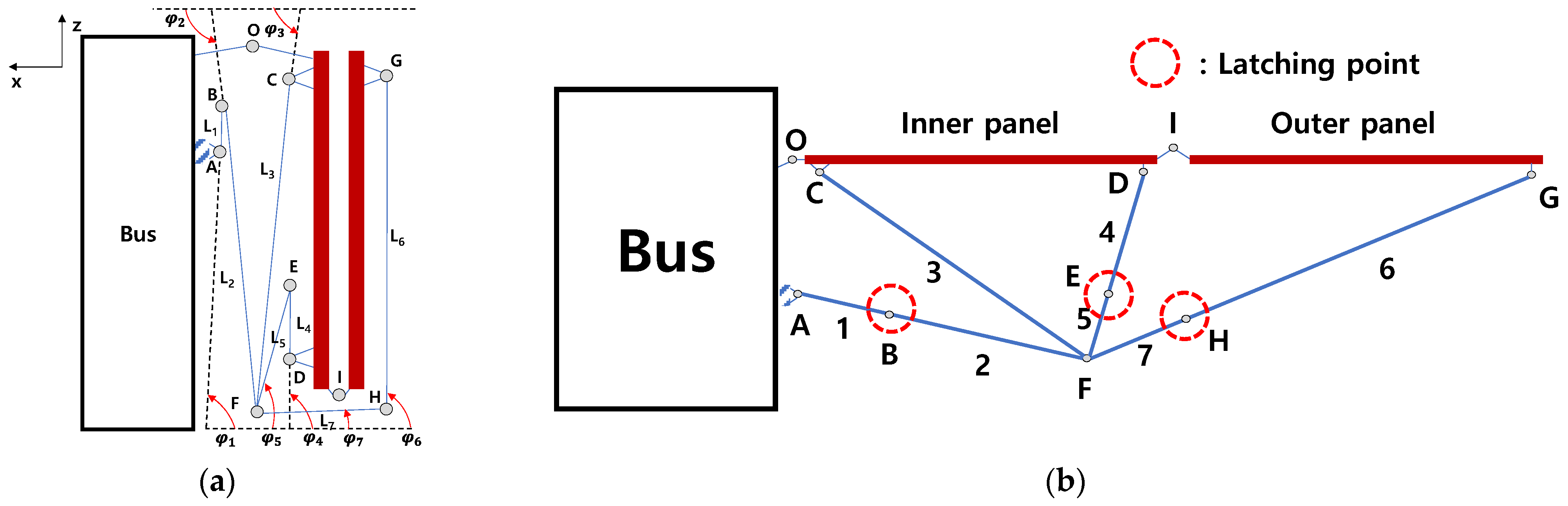
2.2. Configuration Design

The configuration is simplified to a two-dimensional domain to obtain the truss-link’s dimensions in the stowed configuration (Figure 2). By simplifying to a two-dimensional geometry, it is possible to reduce the DOF and variables used to obtain dimensions and coordinates of the body compared to traditional three-dimensional (3D) methods. The dimensions and coordinates were defined in the formula in the reference [23], which was derived using geometric construction methods and bar-groups methods. Upon verification of the formula’s results, it was found that there were some errors, which were fixed accordingly in this study as presented in Equations (2)–(10).
With the panel folded, the length and angle of each truss-link are derived from input variables in Table 2 and Table 3. Input variables including φ1, φ4, φ6, L1, L4, L6, XA, XC, XD, XF, and XG are defined by the mechanical designer considering the size of the panel according to the design requirements. Through Equations (2)–(10), output variables, including φ2, φ3, φ5, φ7, L2, L3, L5, L7, XB, XE, and XH, were determined.
Joint O corresponds to the origin of absolute coordinates as the rotation center of the hinge installed between the bus and the inner panel; Joint I is the rotation center between the inner panel and outer panel; Joint F is the intersection point of all truss-links. Furthermore, to keep the deployment state, three latching points, B, E, and H, were considered, as shown in Figure 2b.
L 3 = ( x F x C ) 2 + ( z F z C ) 2 2
( x H , z H ) = ( x G + L 6 cos φ 6 , z G L 6 sin φ 6 )
L 7 = ( x F ( x G + L 6 cos φ 6 ) ) 2 + ( z F ( z G L 6 sin φ 6 ) ) 2 2
( x B , z B ) = ( x A L 1 cos φ 1 , z A + L 1 sin φ 1 )
L 2 = ( x A L 1 cos φ 1 ) x F ) 2 + ( z A + L 1 sin φ 1 ) z F ) 2 2
φ 2 = cos 1 ( x B x F L 2 )
( x E , z E ) = ( x D L 4 cos φ 4 , z D + L 4 sin φ 4 )
L 5 = ( x D L 4 cos φ 4 ) x F ) 2 + ( z D + L 4 sin φ 4 ) z F ) 2 2
φ 3 = cos 1 ( x F x C L 3 )
φ 5 = cos 1 ( x F x E L 5 )
φ 7 = cos 1 ( x F x H L 7 )
For practical design, a 3D configuration design was conducted by CATIA. The 3D model consists of an inner panel, an outer panel, and 12 truss-links, with dimensions of 1620 mm × 800 mm in the fully deployed configuration (see Figure 3) and a total mass of 11.45 kg as shown in Table 4. The mass of hinges is included in the mass of the panel, and the mass of the bracket is included in the mass of each link. The truss-links connection was finally realized as illustrated in Figure 4a, with several connection angles, as shown in Figure 4b. The connection angles according to the truss-links are summarized in Table 5. The material of the truss-link is aluminum 6061, which has a Young’s modulus of 68.9 GPa, a Poisson’s ratio of 0.33, and density of 2700 kg/m3 [24]. The cross-section of the truss was assumed as a tube-type with an outer diameter of 10 mm and an inner diameter of 8 mm.

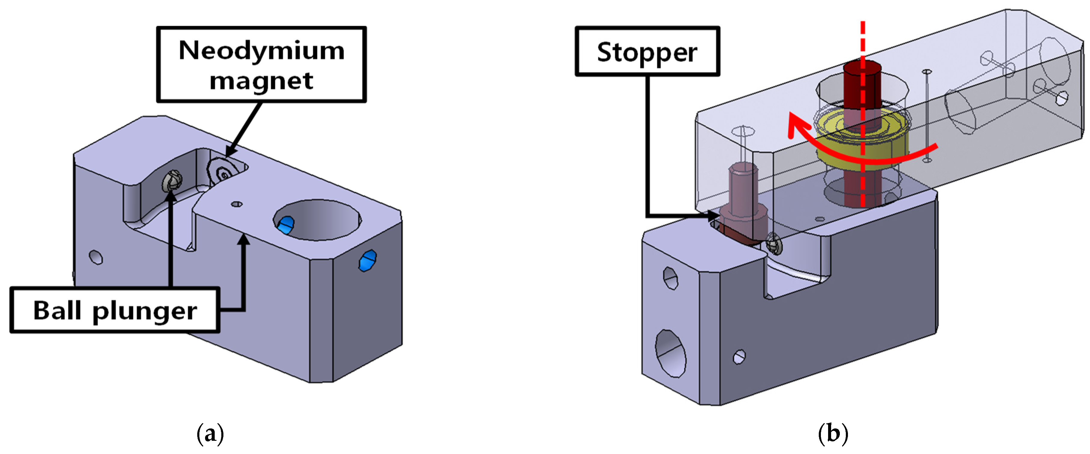
2.3. Latching Mechanism

Once the truss-links are deployed, they must keep their positions and angles through proper latching mechanisms, which are the most critical factors in maintaining the deployment configuration. As shown in Figure 5, the latching structure consists of a neodymium magnet, a ball plunger, and a stopping protrusion. The neodymium magnet and the ball plunger are installed on the lower bracket, and the stopping protrusion is installed on the upper bracket. If the truss-links rotate, the stopping protrusion meets the ball plunger, slides over the ball plunger and locks. In addition, neodymium magnets were installed on the wall to prevent the stopping protrusion from bouncing by the reaction force.

3. Deployment Dynamics

3.1. Modeling of Kinematic Joints and Latching Mechanism

To present the deployment motion, dynamic modeling was conducted with the aid of commercial multibody dynamics (MBD) software, RecurDyn. There were three kinds of joints: revolute joints for one-axis revolution, fixed joints to eliminate rigid-body motion, and on-off joints for latching truss-links. In contrast to the two-dimensional type-2 design, in the actual 3D design, when many truss-links were connected at a rotation joint (see Figure 4a) such as joint F, the over-constrained mechanisms cannot be avoided according to Equation (1). To address this problem, we used the bushing force function of RecurDyn instead of the revolute joint [25]. The bushing force can model any joint with 6 DOF by adjusting the stiffness of six springs independently. In the case of a revolute joint with the bushing force, the translation stiffness was set to be sufficiently high that the translation motion would be constrained; one of the rotational stiffnesses was set to zero for the revolution while the other rotation stiffness was set high. The proposed truss-link mechanism must be latched on each joint, B, E, and H, in a fully deployed state at the end of the deployment process. The on/off joints provided by RecurDyn are used to address these problems, which allows operation when certain conditions are met [26], as shown in Table 6. Using this, we modeled the two links connected to the joint to be fixed without generating additional motion when they are aligned.

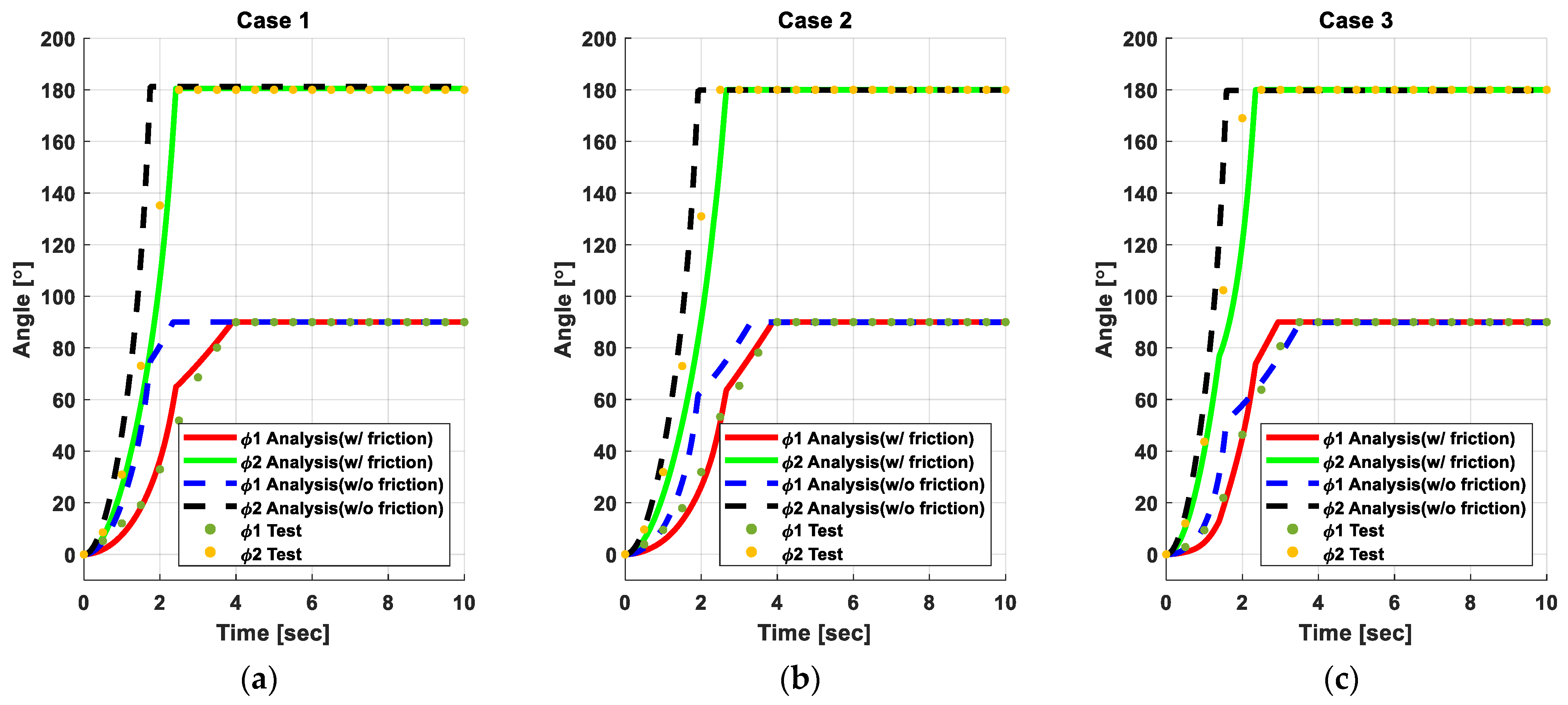
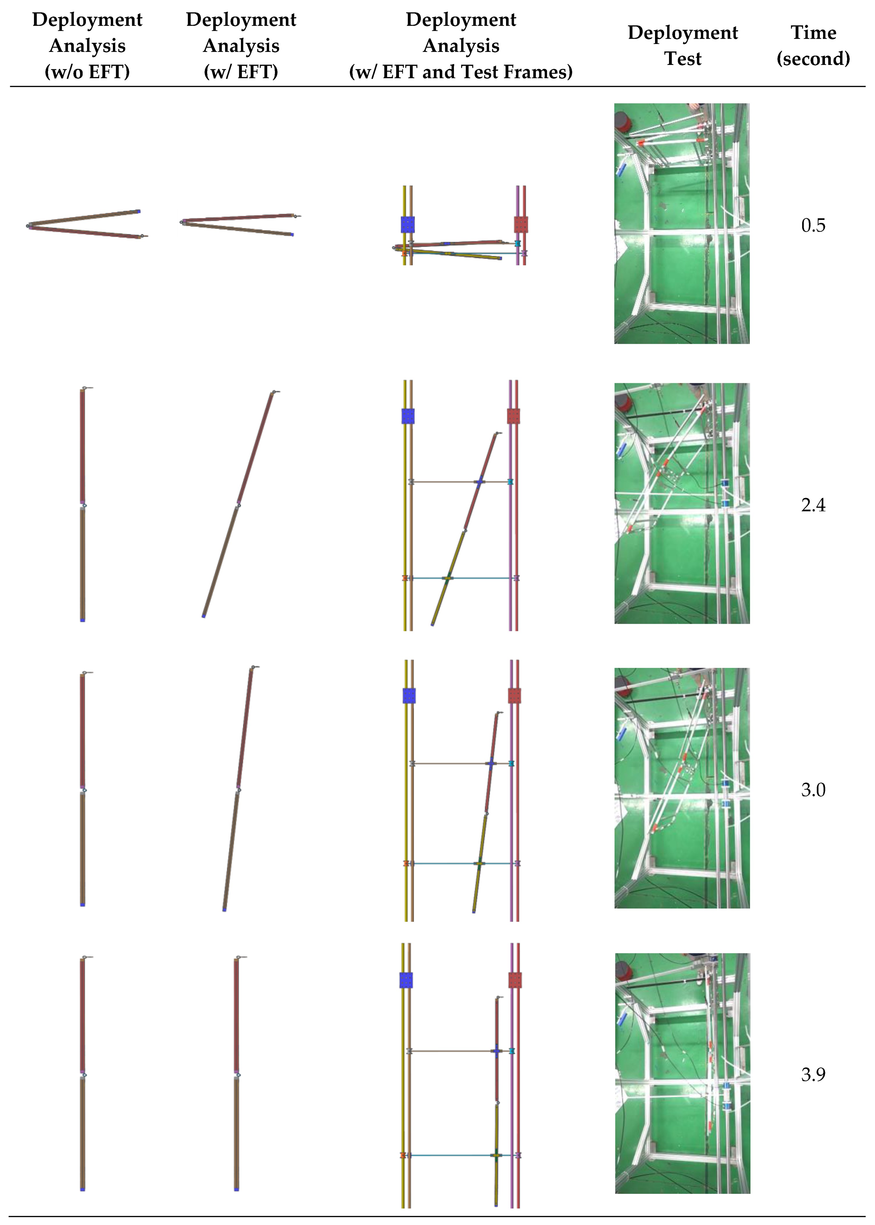
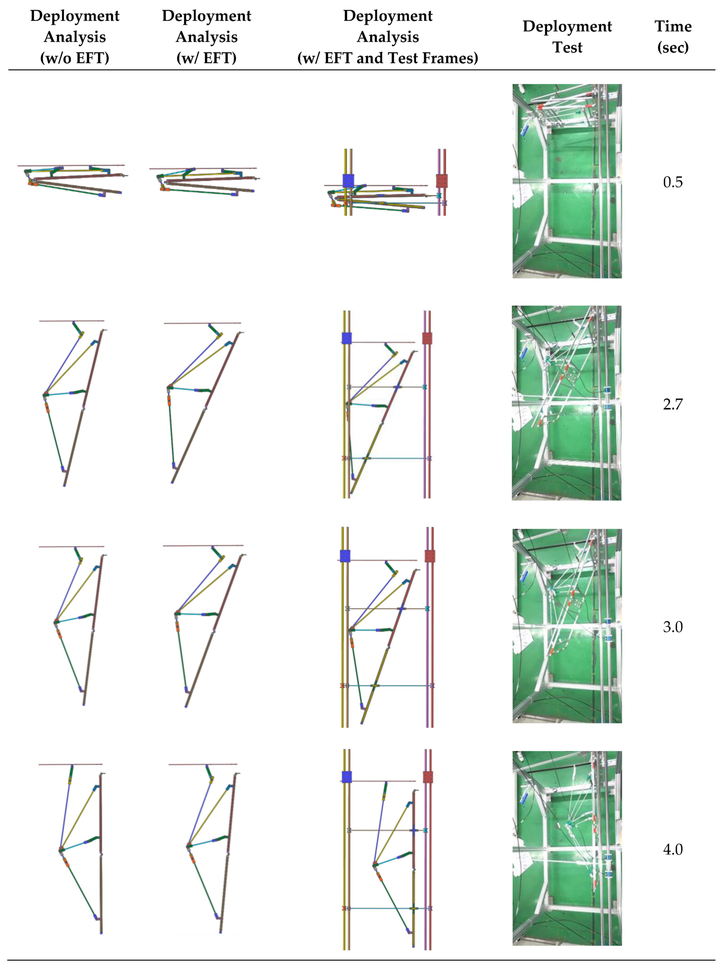
3.2. Deployment Dynamics Analysis
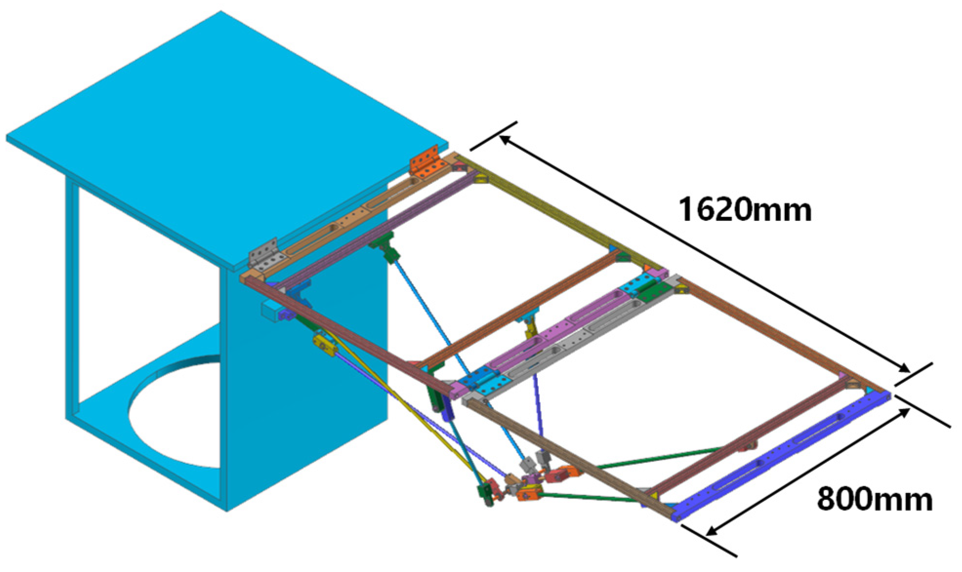
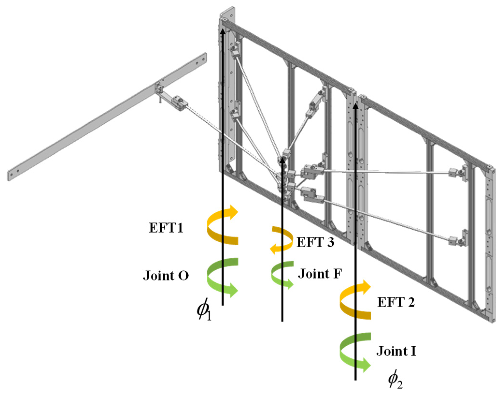
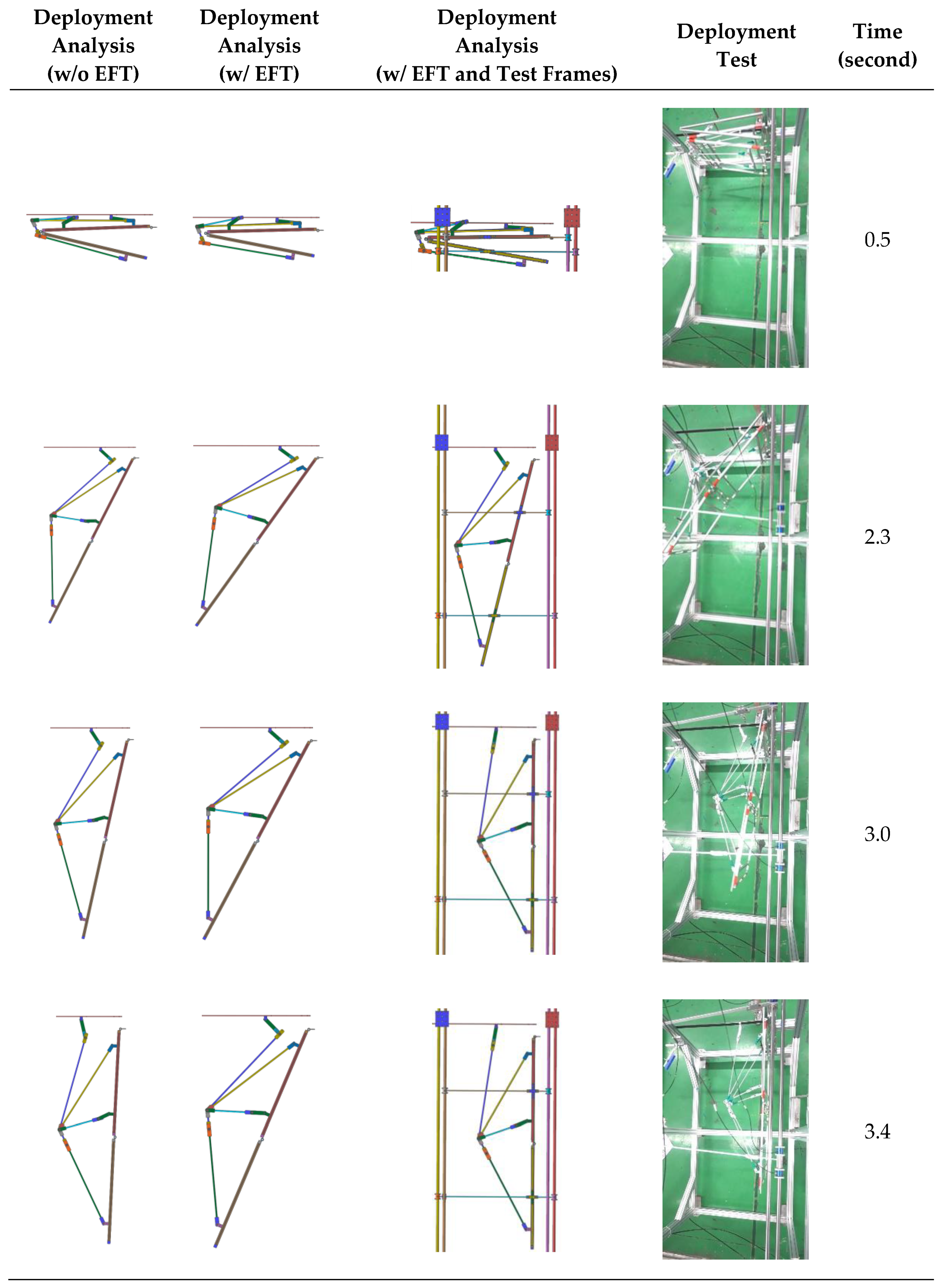
Deployment behavior was analyzed by RecurDyn. Table 7 shows the mass properties of the two panels, and Figure 6 shows the rotational stiffness of the 90° and 180° torsional spring hinges, which were measured and realized through the spline function of RecurDyn [23]. The initial rotation angles were set to 90° and 180°, respectively, forcing the rotation joints to have driving torques in the stowed configuration.

4. Deployment Test

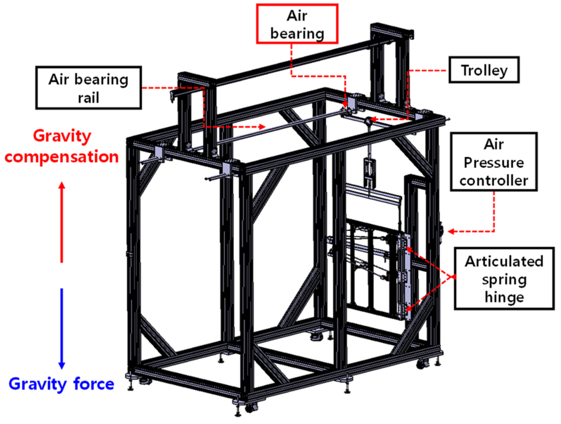
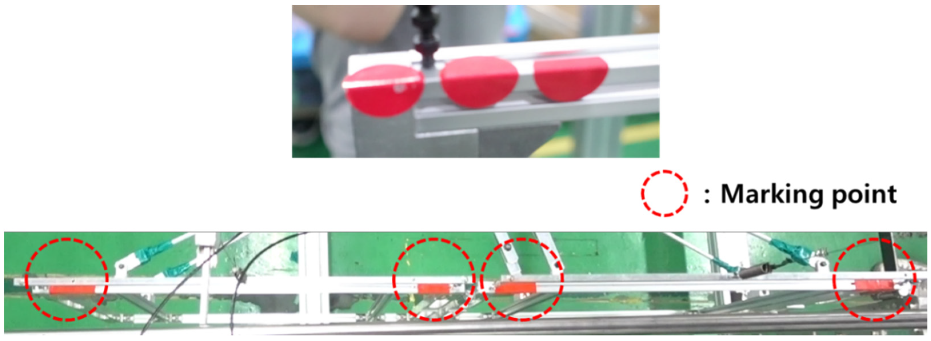
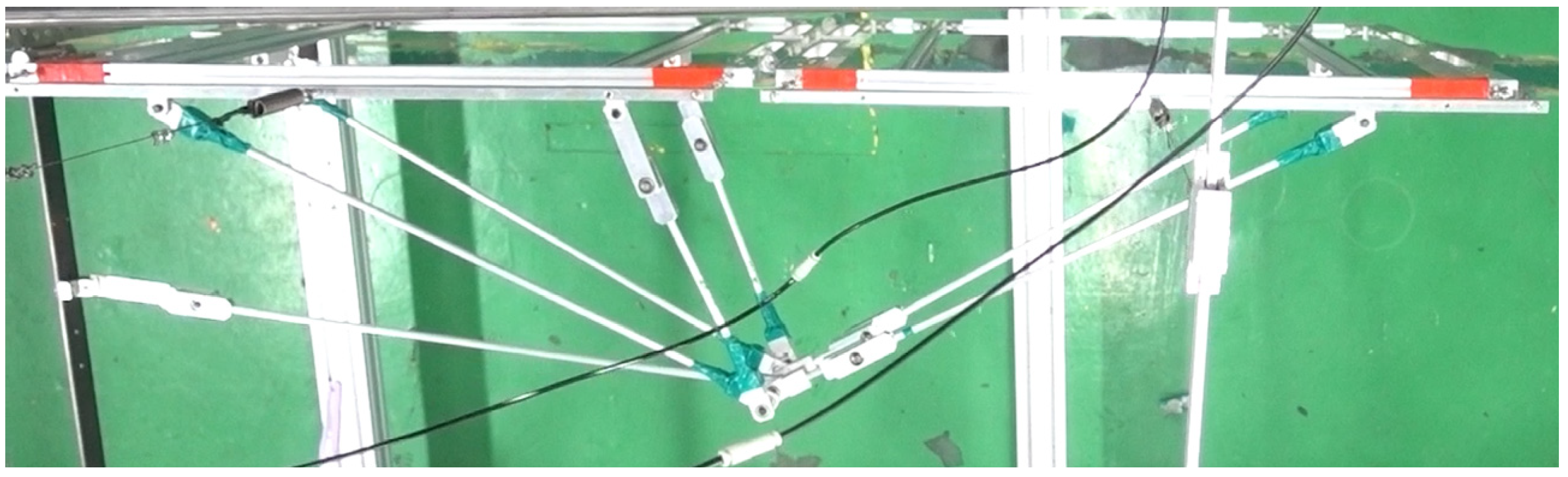
4.1. Test Configuration and Test Cases

Dummy panels accommodating rotational torsion spring hinges between panels were established to verify the design of the deployment performance. To make a weightless environment for structures, a zero-G device was used [27] by hanging the structure with spring-loaded wires to minimize deflection and friction against gravity on the air bearings (Figure 7). Before the test, alignment of the test fixture was adjusted within 0.01° using a two-axis digital protractor, to place the panel close to horizontal from the ground. As shown in Table 8, three test cases were chosen to determine whether the panel was fully deployed according to changes of the driving torque. The video camera was installed at the ceiling of the test facility. During the tests, we employed a set of red markers on top of the frames to record the deployment angle history of the inner and outer panels using the MATLAB color extraction algorithm (see Figure 8). Finally, the locations of color were used to evaluate the angles of panels using inverse kinematics from the position history. The deployment test showed the dummy panels were fully deployed with the joints of each truss-link latched successfully (see Figure 9).

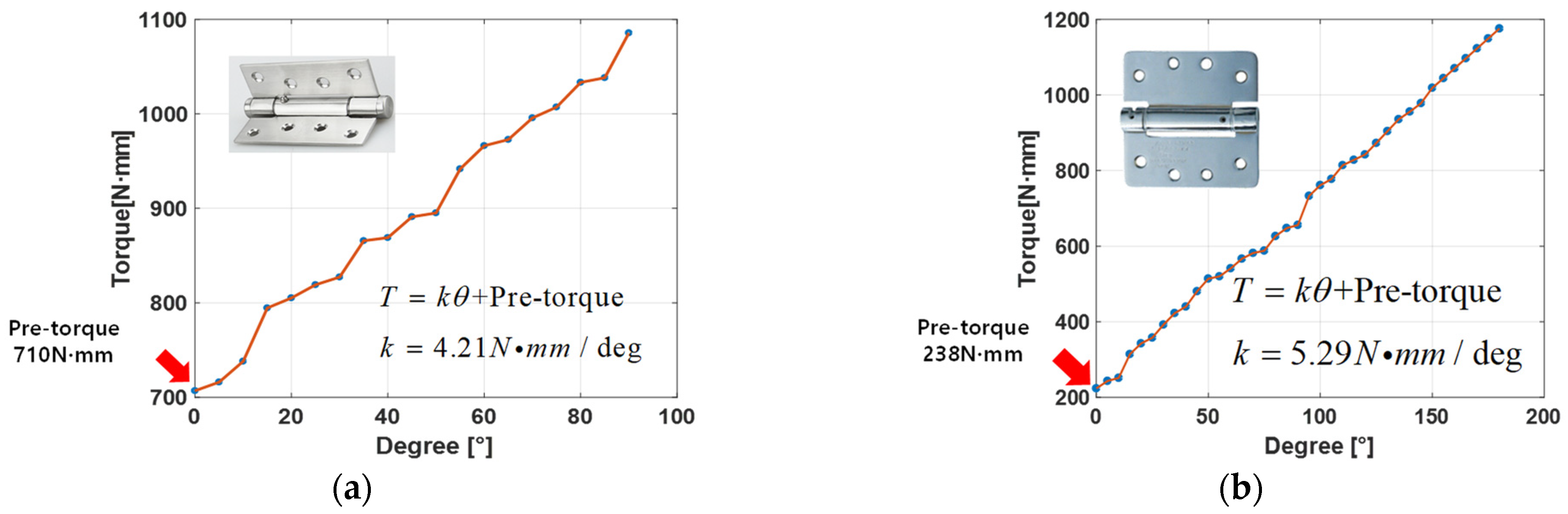
4.2. Modeling of Friction and Trajectory Error

For friction compensation, a rotational friction model considering the Coulomb friction torque was employed as given below [27,28]:
E F T T C tanh ( ω ω c o u l )
where T C , ω and ω C o u l are the Coulomb friction torque, relative angular velocity, and Coulomb threshold velocity, respectively; ω C o u l is a parameter used to alleviate numerical instability caused by Coulomb friction. In this work, 0.01 rad/s was used as the reference value [28]. As seen in Figure 10, EFT1, EFT2, and EFT3 are the equivalent friction torques at joints O, I, and F; ϕ 1 and ϕ 2 indicate the rotation angles of joint O and I; trajectory error was defined and computed using Equation (14) as follows:
T r a j e c t o r y   e r r o r ( ϕ a ) = 1 n t = 0 n ( ϕ e ( t i ) ϕ a ( t i ) ϕ e ( t i ) × 100 )
where ϕ a = ϕ a ( E F T 1 , E F T 2 , E F T 3 , t ) in degrees are the rotation angles according to the time evolution; the initial time was t 0 = 0   s and the time step Δ t = 0.05   s ; n , a , e denote the number of time data used, analysis, and experiment, respectively. The data were compared for four seconds until all panels were fully deployed in the test. We added the test frames in the MBD model to consider the effect of test fixture. Contact stiffness of 37,000 N/mm1.5 and contact damping of 3.7 N∙s/mm1.25 were applied based on Hertz contact theory [29] between panel to panel and between truss-links to panels to allow for movement within a limited area in case of contact.

4.3. Response Surface Methodology for Friction Identification

From comparison results between the test and simulation, as shown in Figure 11, it was observed that all simulations deployed earlier than those of the test. This is believed to be caused by a slight misalignment of the test frame, friction at the joints, and air drag from the panels and truss-links during the deployment test. Therefore, we attempted to adjust the deployment simulation model by adding the equivalent friction torques (EFT) at the three revolute joints defined as EFT1, EFT2, and EFT3, including those from all sources of friction, as defined in Figure 10. The EFT values can be easily determined by solving an optimization problem with the response surface method (RSM), making the rotation angle history of the analysis results similar to that of the test. The response surface y was generated with three design parameters, as in Equation (15). It is a polynomial function having ten terms corresponding to unknown coefficients, and the optimal response is found through the response function.
y = β 0 + β 1 x 1 + β 2 x 2 + β 3 x 3 + β 12 x 1 x 2 + β 13 x 1 x 3 + β 23 x 2 x 3 + β 11 x 1 2 + β 22 x 2 2 + β 33 x 3 2
where x i , β i and β i j are the values of the design variables and the coefficients of the polynomials of design variables, respectively. Here, the design variables indicate the equivalent friction torques: EFT1, EFT2, and EFT3. To determine the coefficients of the polynomials, 15 design cases were determined by the central composite design, popularly adopted in the design of experiments (DOE). The response variables were assigned to the trajectory error of the angles history of the inner panel (90°) at joint O and the outer panel (180°) at joint I. After deployment simulation for 15 design cases for test case 2, two output responses were computed and summarized, shown in Table 9. Finally, the coefficients of the polynomials of design variables were determined by regression analysis. To check the suitability of the derived response surface, R 2 (coefficient of determination) was obtained as 0.978, indicating a high correlation between the design variables and response variables. By determining the minimum point of the response surface, it was found that EFT1, EFT2, and EFT3 were 0.54 N∙m, 0.472 N∙m, and 0.065 N∙m, respectively, showing an excellent correlation between the test and analysis for test case 2 with the corresponding trajectory error 1 and 2 as 7.69%, 6.62%, respectively, as presented in Figure 11b. The coefficients of the polynomials were obtained in the Equation (16).
β = [ β 0 , β 1 , β 2 , β 3 , β 12 , β 13 , β 23 , β 11 , β 22 , β 33 ] = [ 16.329 ,   3.713 ,   1.703 ,   1.107 ,   0.823 ,   1.290 ,   0.658 ,   2.040 ,   1.529 ,   1.262 ]
Although there remains a slight gap between the analysis and the test after friction compensation, this is explained by all the sources of friction occurring in the test which cannot be considered. In addition, these EFT values were applied in test case 1 and test case 3, which additionally produce a good correlation between the test and analysis, as shown in Figure 11a,c. A detailed comparison is summarized in Figure 12, Figure 13 and Figure 14.

4.4. Torque Margin Evaluation

From the deployment test result, for all test cases the deployment of the truss-link mechanism was successful. However, we re-validated the EFTs with torque margin analysis [30]. If the torque margin was negative, the deployment would fail due to inadequate driving torque. If the torque margin was positive, the selected driving torque would be appropriate and completely deployed. To analyze this phenomenon, the torque margin was calculated as
E D 90 ° = 0 π 2 T D d θ
E D 180 ° = 0 π T D d θ
E R 90 ° = 0 π 2 T R d θ
E R 180 ° = 0 π T R d θ
T o r q u e M a r g i n = ( E D E R 1 ) × 100 ( % )
where T D , T R are the driving torque and the resistance torque of Joint O (90°) and Joint I (180°), respectively. Moreover, E D , E R are the driving torque energy and the resistance torque energy value of Joint O and Joint I. The torque margin calculation results for Joint O and I are summarized in Table 10 and Table 11. If the torque margin value was negative, then the deployment of panels at the corresponding joints would not be achieved. For the test cases, all torque margin values were positive. As seen in Figure 12, Figure 13 and Figure 14, all the test cases were fully deployed. Through this evaluation, it can be predicted that the worst case cannot be deployed in advance. Therefore, the EFT estimation method developed in this work was verified with excellent reliability.

5. Conclusions

In this paper, the modeling and validation of a passive truss-link mechanism applicable to a large-scale deployable structure for small satellites were designed to achieve a successful deployment. To design the truss-link mechanism, we referred to the truss-link structure of RADARSAT-2 satellites. A detailed design of the 3D truss-link structure followed based on the 2D configuration defined by the equations consisting of geometric construction methods and bar-groups methods.
Note that in contrast to the many truss-link mechanisms [11,12,13,14,15,16,17], we do not accommodate any active driving mechanisms as they lack simplicity, are not highly reliable, and are expensive. As driving mechanisms, only conventional torsion spring hinges with proper latching mechanisms were employed in this work.
To demonstrate the performance of the deployable structure with truss-links, a deployment simulation with the MBD model was conducted with proper joint modeling and rotational spring stiffness. Furthermore, a deployment test was conducted to check the correlation between the test and analysis. The results revealed that the time history of the deployment test was slightly behind that of the deployment analysis. To compensate for this, an inverse identification technique for equivalent friction torque (EFT) was proposed based on the results of the response surface method combined with the central composite design technique. Finally, with the EFTs, the angular rotation history in the deployment analysis was much closer to that of the deployment test with a trajectory error of less than 8%. Therefore, the adequacy of the proposed design of the deployable structure with truss-links was verified. This kind of truss-links mechanism has strong potential to extend a multi-modular deployable structure for small satellites. It will be further discussed in our future works.

Author Contributions

Conceptualization, J.H.L.; methodology, H.-S.C., T.S.J.; software, J.-H.P., H.-S.C.; validation, H.-S.C., J.-H.P.; investigation, D.-Y.K., H.-S.C.; data curation, H.-S.C.; writing—original draft preparation, J.H.L.; writing—review and editing, T.S.J.; supervision, J.H.L. All authors have read and agreed to the published version of the manuscript.

Funding

This research was supported by the National Research Foundation of Korea (NRF) funded by the Ministry of Science and ICT (NRF-2018M1A3A02065478).

Institutional Review Board Statement

Not applicable.

Informed Consent Statement

Not applicable.

Data Availability Statement

Not applicable.

Conflicts of Interest

The authors declare no conflict of interest.

References

  1. Kim, S.-Y. SAR Antenna Technology. In Proceedings of the Korea Electromagnetic Engineering Society, Ilsan, Korea, 25 November 2011. [Google Scholar]
  2. Park, T.-Y.; Kim, S.-Y.; Yi, D.-W.; Jung, H.-Y.; Lee, J.-E.; Yun, J.-H.; Oh, H.-U. Thermal Design and Analysis of Unfurlable CFRP Skin-Based Parabolic Reflector for Spaceborne SAR Antenna. Int. J. Aeronaut. Space Sci. 2021, 22, 433–444. [Google Scholar] [CrossRef]
  3. Kim, D.-Y.; Lim, J.H.; Jang, T.-S.; Cha, W.H.; Lee, S.-J.; Oh, H.-U.; Kim, K.-W. Optimal design of stiffness of torsion spring hinge considering the deployment performance of large scale sar antenna. J. Aerosp. Syst. Eng. 2019, 13, 78–86. [Google Scholar]
  4. Hoffait, S.; Brüls, O.; Granville, D.; Cugnon, F.; Kerschen, G. Dynamic analysis of the self-locking phenomenon in tape-spring hinges. Acta Astronaut. 2010, 66, 1125–1132. [Google Scholar] [CrossRef]
  5. Kim, K.-W.; Park, Y. Systematic design of tape spring hinges for solar array by optimization method considering deploy-ment performances. Aerosp. Sci. Technol. 2015, 46, 124–136. [Google Scholar] [CrossRef]
  6. Lee, Y.; Lee, J.E.; Kim, M.-G.; Jung, S.Y. A Study of a Mobile Launch Platform Effect on Bi-folded Wing Deployment. Int. J. Aeronaut. Space Sci. 2021, 22, 560–566. [Google Scholar] [CrossRef]
  7. Calassa, M.C.; Kackley, R. Solar Array Deployment Mechanism. In Proceedings of the 29th Aerospace Mechanisms Symposium, Pasadena, CA, USA, 17–19 May 1995. [Google Scholar]
  8. Cha, W.-H.; Seo, J.-K.; Jang, T.-S.; Lee, S.Y.; Chae, J.-S.; Shin, G.-H.; Lee, S.-H.; Ryu, K.-S.; Kim, D.-K. NEXTSat-1 Solar Panel Deployment Device Test. In Proceedings of the Korean Society for Aeronautical and Space Sciences, Jeju-si, Korea, 18–20 November 2015. [Google Scholar]
  9. Kim, K.-W.; Park, Y. Solar array deployment analysis considering path-dependent behavior of a tape spring hinge. J. Mech. Sci. Technol. 2015, 29, 1921–1929. [Google Scholar] [CrossRef]
  10. Jeong, J.W.; Yoo, Y.I.; Shin, D.K.; Lim, J.H.; Kim, K.W.; Lee, J.J. A novel tape spring hinge mechanism for quasi-static deployment of a satellite deployable using shape memory alloy. Rev. Sci. Instrum. 2014, 85, 025001. [Google Scholar] [CrossRef] [PubMed]
  11. Lin, F.; Chen, C.; Chen, J.; Chen, M. Dimensional synthesis of antenna-deployable support structure. Int. J. Aeronaut. Space Sci. 2020, 21, 404–417. [Google Scholar] [CrossRef]
  12. Francis, R.; Graf, G.; Edwards, P.G.; McCaig, M.; McCarthy, C. The ers-1 spacecraft and its payload. ESA Bull. 1991, 65, 26–48. [Google Scholar]
  13. Ahmed, S.; Parashar, S.; Langham, E.; McNally, J. RADARSAT Mission Requirements and Concept. Can. J. Remote Sens. 1993, 19, 280–288. [Google Scholar]
  14. Thomas, W.D.R. RADARSAT-2 extendible support structure. Can. J. Remote Sens. 2004, 30, 282–286. [Google Scholar] [CrossRef]
  15. Thompson, A.A. Overview of the RADARSAT Constellation Mission. Can. J. Remote Sens. 2015, 41, 401–407. [Google Scholar] [CrossRef]
  16. Kankaku, Y.; Suzuki, S.; Osawa, Y. ALOS-2 mission and development status. In Proceedings of the 2013 IEEE International Geoscience and Remote Sensing Symposium—IGARSS, Melbourne, Australia, 21–26 July 2013. [Google Scholar]
  17. Born, G.H.; Dunne, J.A.; Lame, D.B. Seasat Mission Overview. Science 1979, 204, 1405–1406. [Google Scholar] [CrossRef] [PubMed]
  18. The European Space Agency. Earth Online. Available online: https://earth.esa.int/eogateway/missions/worldview-4 (accessed on 11 November 2021).
  19. The European Space Agency. Sentinel-5p. Available online: https://www.esa.int/Applications/Observing_the_Earth/Copernicus/Sentinel-5P (accessed on 11 November 2021).
  20. Wang, Y.; Deng, Z.; Liu, R.; Yang, H.; Guo, H. Topology Structure Synthesis and Analysis of Spatial Pyramid Deployable Truss Structures for Satellite SAR Antenna. Chin. J. Mech. Eng. 2014, 27, 2014. [Google Scholar] [CrossRef]
  21. Han, B.; Xu, Y.; Yao, J.; Zheng, D.; Guo, L.; Zhao, Y. Type synthesis of deployable mechanisms for ring truss antenna based on constraint-synthesis method. Chin. J. Aeronaut. 2020, 33, 2445–2460. [Google Scholar] [CrossRef]
  22. Uicker, J.J. Theory of Machines and Mechanisms, 5th ed.; OXFORD University Press: New York, NY, USA, 2017; pp. 12–17. [Google Scholar]
  23. Xu, Y.; Lin, Q.; Wang, X.; Li, L.; Cong, Q.; Pan, B. Mechanism Design and Dynamic Analysis of a Large-Scale Spatial Deployable Structure for Space Mission. In Proceedings of the Seventh International Conference on Electronics and Information Engineering, Nanjing, China, 17–18 September 2017. [Google Scholar]
  24. ASTM B209M, Standard Specification for Aluminum and Aluminum-Alloy Sheet and Plate (Metric); ASTM International: West Conshohocken, PA, USA, 21 November 2014.
  25. Available online: https://support.functionbay.com/ko/faq/single/79/revolute-joint-modeling-using-bushing-force (accessed on 8 October 2021).
  26. FunctionBay, Recurdyn/Solver Theoretical Manual. Available online: https://functionbay.com/documentation/onlinehelp/default.htm#!Documents/introduction.htm (accessed on 8 October 2021).
  27. Kim, D.-Y.; Choi, H.-S.; Lim, J.H.; Kim, K.-W.; Jeong, J. Experimental and Numerical Investigation of Solar Panels Deploy-ment with Tape Spring Hinges Having Nonlinear Hysteresis with Friction Compensation. Appl. Sci. 2020, 10, 7902. [Google Scholar] [CrossRef]
  28. Armstrong, B.; De Wit, C.C. Friction modeling and compensation. Control. Handb. 1996, 77, 1369–1382. [Google Scholar]
  29. Barber, J.R. Contact Mechanics; Springer: Cham, Switzerland, 2018; pp. 29–40. [Google Scholar]
  30. Postma, R.W. Force and Torque Margins for Complex Mechanical Systems. In Proceedings of the 37th Aerospace Mechanisms Symposium, Galveston, TX, USA, 18–21 May 2014; pp. 107–118. [Google Scholar]
Figure 1. Configuration of 2-D truss-link mechanism: (a) Type 1 (RADARSAT-1) (b) Type 2 (RADARSAT-2).
Applsci 12 00451 g001
Figure 2. Configuration design of truss-link mechanism in (a) stowed configuration (b) deployed configuration with latching points: B, E, H.
Applsci 12 00451 g002
Figure 3. Configuration of a deployment analysis model.
Applsci 12 00451 g003
Figure 4. Configuration of truss-link mechanism: (a) 3-D truss, (b) truss-links with connection angles θ.
Applsci 12 00451 g004
Figure 5. Configuration of latching mechanism: (a) Neodymium magnet, ball plungers (b) Latching system.
Applsci 12 00451 g005
Figure 6. Configuration of rotational spring hinges and the relationship between torque and rotation angles: (a) 90° hinge (Joint O), (b) 180° hinge (Joint I).
Applsci 12 00451 g006
Figure 7. Test configuration of panels with truss-link mechanism [27].
Applsci 12 00451 g007
Figure 8. Configuration of red markers on dummy panels.
Applsci 12 00451 g008
Figure 9. Fully deployed configuration (case 2 and case 3).
Applsci 12 00451 g009
Figure 10. Definition of the equivalent friction torques.
Applsci 12 00451 g010
Figure 11. Comparison of the rotation angle history between test and analysis before/after friction compensation: (a) case 1, (b) case 2, (c) case 3.
Applsci 12 00451 g011
Figure 12. Comparison of the deployed motion history for case 1.
Applsci 12 00451 g012
Figure 13. Comparison of the deployed motion history for case 2.
Applsci 12 00451 g013
Figure 14. Comparison of the deployed motion history for case 3.
Applsci 12 00451 g014
Table 1. Evaluation of total DOF.
Type 1
(RADARSAT-1)
Type 2
(RADARSAT-2)
Body (L)Bus (1) + Links (11) = 12Bus (1) + Links (9) = 10
J1, J2J1 = 12, J2 = 0J1 = 10, J2 = 0
Degrees of freedom3 × (12 − 1) − 2 × (12) = 93 × (10 − 1) − 2 × (10) = 7
Table 2. Design variables of the truss-link mechanism.
InputOutput
Angle variablesφ1, φ4, φ6φ2, φ3, φ5, φ7
Length variablesL1, L4, L6L2, L3, L5, L7
Absolute coordinate variablesA, C, D, F, GB, E, H
Table 3. Values of the input and output design variables of truss-link mechanism.
Input VariablesValueOutput VariablesValue
φ191.55°φ293.11°
φ4129.18°φ391.64°
φ692.06°φ5104.20°
L1140.00 mmφ727.77°
L486.00 mmL2726.28 mm
L6661.34 mmL3753.58 mm
XA(57.00, −288.00) L5309.38 mm
XC(43.00, −120.00)L7129.54 mm
XD(43.00, −640.00)XB(60.79, −148.05)
XF(21.44, −873.27)XE(97.34, −573.34)
XG(−69.40, −152.00)XH(−93.18, −812.91)
XO(−13.00, 11.00)XI(−13.20, −813.00)
Table 4. Length and weight of truss-link mechanism.
IDQuantity [ea]Length [mm]Mass [g]
Link 11140.00173.60
Link 21726.28176.86
Link 32753.58370.41
Link 4286.00321.96
Link 52309.38379.38
Link 62661.34437.19
Link 72129.54342.14
Panel2800 × 8008505.47
Panel joints7-447.99
Shaft10-291.31
Total--11,446.31
Table 5. Connection angle of truss-links.
LinkConnection
Angle [°]
LinkConnection
Angle [°]
Link 1180Link 5168
Link 2180Link 6170
Link 3170.5Link 7170
Link 4168
Table 6. Expression function for latching mechanism.
TypeExpression
Applsci 12 00451 i001
On/Off joint
Expression: [AZ(1,2) × RTOD > 180°]
AZ(1,2): Angle between 1 and 2
(1: body 1, 2: body 2)
RTOD: Radian to degree
180°: Latching angle
Table 7. Dimensions and mass properties of inner and outer panels.
Panel 1Panel 2
Mass [kg]4.234.28
Moment of inertia
[kg∙mm2]
w.r.t. C.G.
I x x = 0.81 × 10 6 I x x = 0.81 × 10 6
I y y = 0.36 × 10 6 I y y = 0.36 × 10 6
I z z = 0.45 × 10 6 I z z = 0.45 × 10 6
I x y = 9.18 × 10 3 I x y = 9.52 × 10 3
I y z = 0.52 × 10 1 I y z = 0.21 × 10 1
I z x = 0.99 × 10 1 I z x = 0.45 × 10 1
Dimension800 mm × 800 mm × 20 mm
Table 8. Test cases.
Test-IDJoint OJoint ITruss-Links
Case 12.17 N·m
(2ea)
2.38 N·m
(2ea)
×
Case 22.17 N·m
(2ea)
2.38 N·m
(2ea)
O
Case 32.17 N·m
(2ea)
3.57 N·m
(3ea)
O
Table 9. Design cases of central composite design.
No.Design VariablesResponse Variables
EFT1EFT2EFT3Trajectory Error 1
(%)
Trajectory Error 2
(%)
11.170.600.1028.6520.75
20.751.100.1015.9028.03
30.750.600.1016.3213.07
41.000.300.1525.6915.20
50.330.600.1015.4913.32
60.750.0950.1025.353.66
70.500.900.0511.1022.03
81.000.300.0523.988.73
91.000.900.0524.6421.46
100.500.300.0518.076.70
110.750.600.01619.4613.29
120.500.300.1520.6010.84
131.000.900.1524.6425.36
140.750.600.1820.2815.88
150.500.900.1513.7128.34
Table 10. Driving and resistance torque energy according to the test cases.
Test-IDDriving Torque Energy
[N∙m]
Resistance Torque Energy
[N∙m]
Case 12.8180.848
4.4841.473
Case 22.8180.848
4.4841.476
Case 32.8180.848
6.7261.476
Table 11. Torque margin calculation for all test cases.
Test-IDJointDriving Torque
[N∙m]
Friction Torque
[N∙m]
Torque Margin
[%]
Test
(Pass/Fail)
Analysis
(Pass/Fail)
Case 1Joint O2.170.54232.31PassPass
Joint I2.380.47204.41PassPass
Case 2Joint O2.170.54232.31PassPass
Joint I2.380.47203.80PassPass
Case 3Joint O2.170.54232.31PassPass
Joint I3.570.47355.69PassPass
Publisher’s Note: MDPI stays neutral with regard to jurisdictional claims in published maps and institutional affiliations.

