
Prediction of Compressive Strength of Fly-Ash-Based Concrete Using Ensemble and Non-Ensemble Supervised Machine-Learning Approaches

 , , , , and
Abstract
:1. Introduction
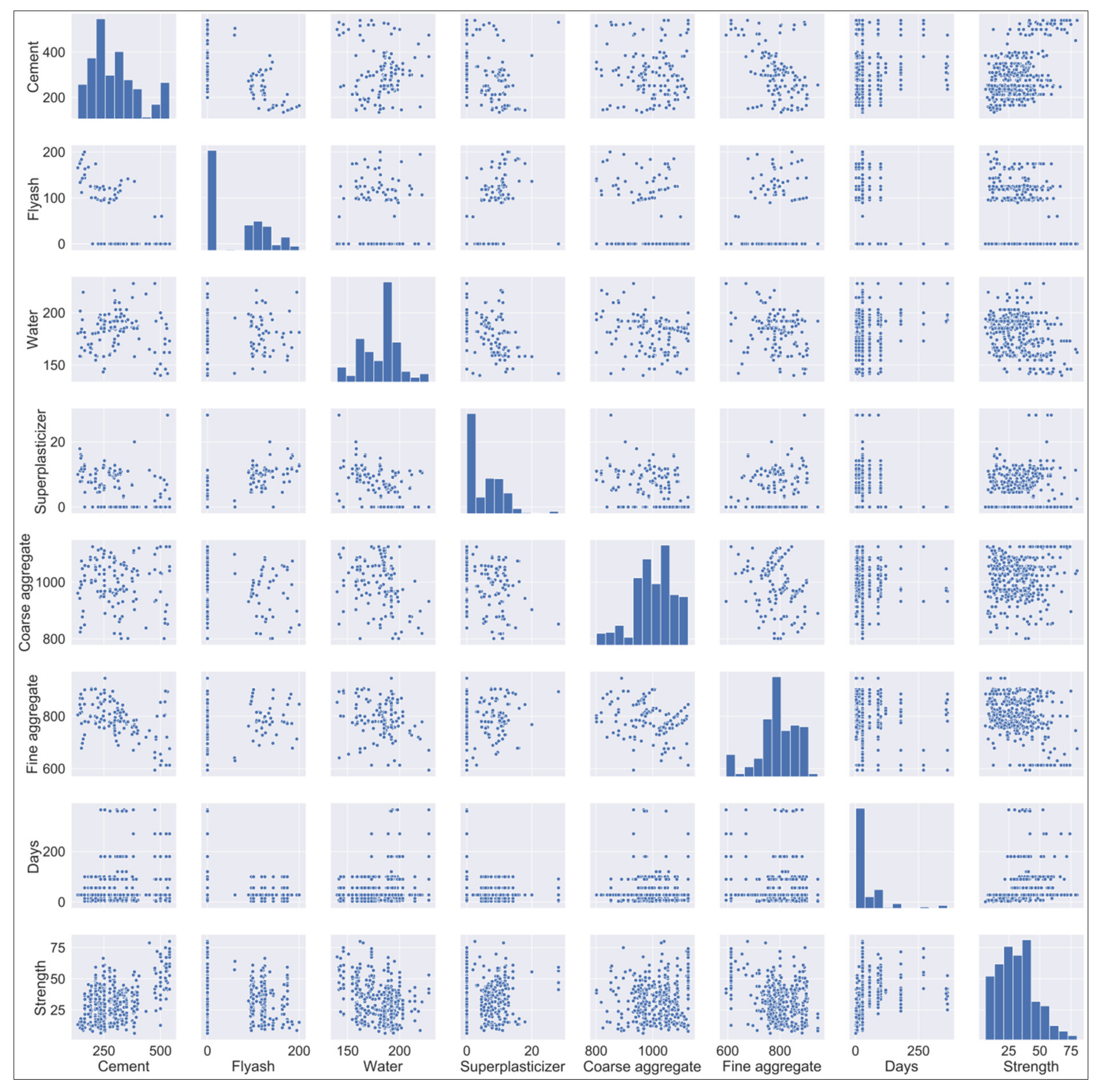
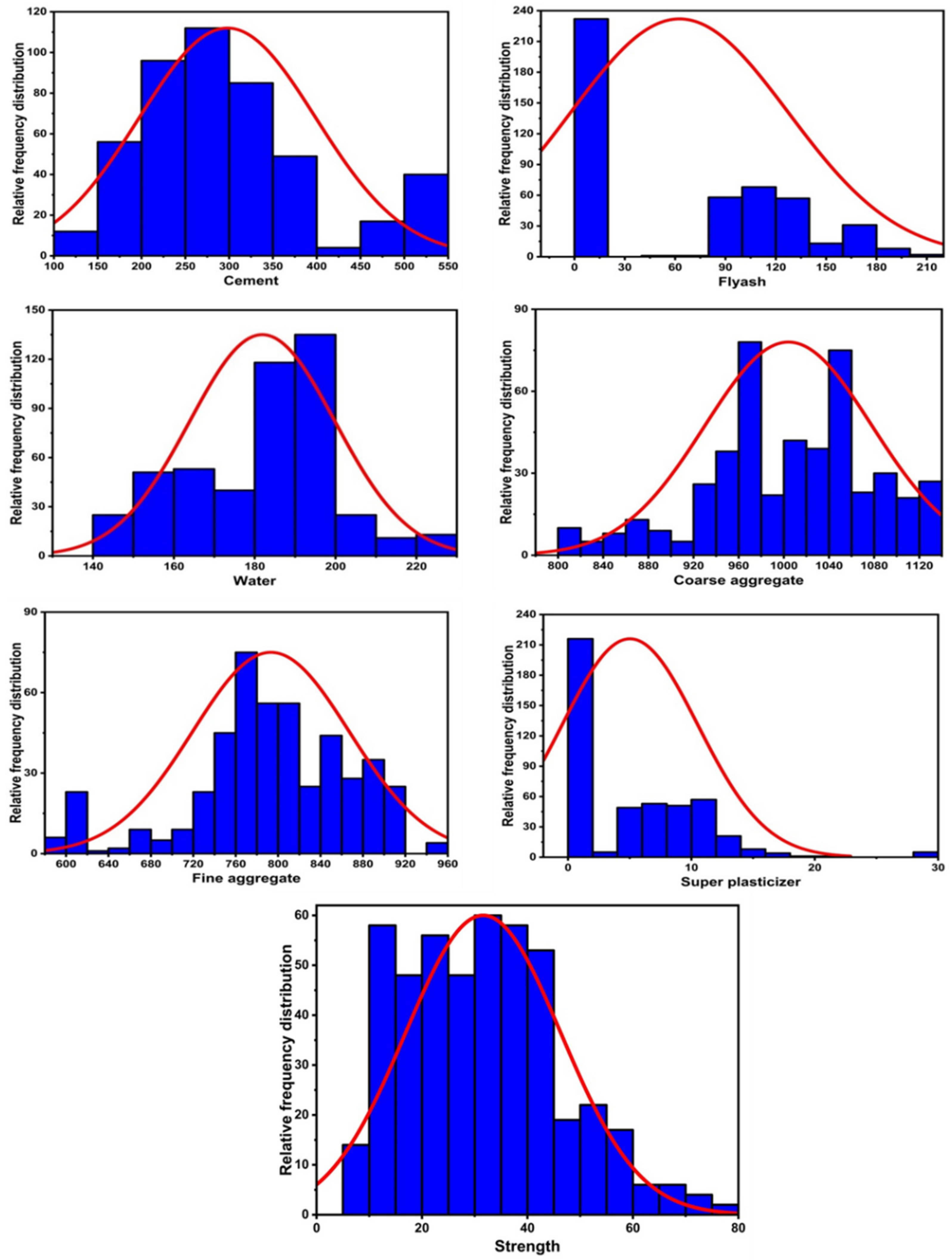
2. Database Description
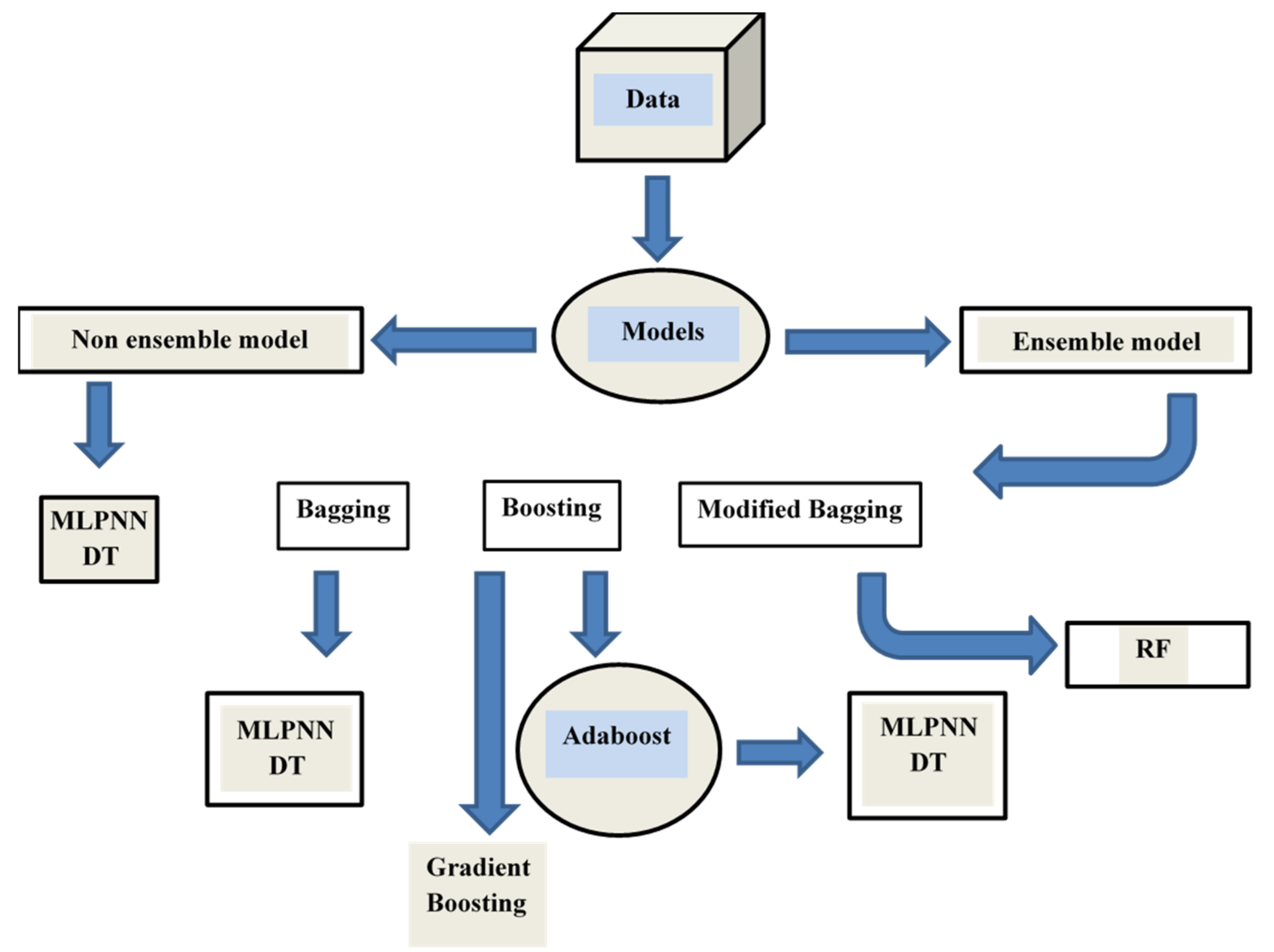
3. Machine Learning Methods
3.1. Overview of Machine Learning Algorithms
3.1.1. DT Algorithm
3.1.2. Random Forest (RF) Regressor
- The frame of the given data is two-thirds of the total data collected randomly for each tree. This is referred to as bagging. Forecasted parameters are chosen freely and the node-splitting algorithm uses the finest split on these parameters.
- For each tree, the out-of-bag error is determined using the remaining data. Additionally, errors from each tree are accumulated to determine the ultimate out-of-bag error rate.
- Each tree displays a regression, and the model chooses the prediction with the most votes out of all the trees in the forest. These can be zeroes or ones. Forecasting probability is defined as the proportion of 1’s obtained.
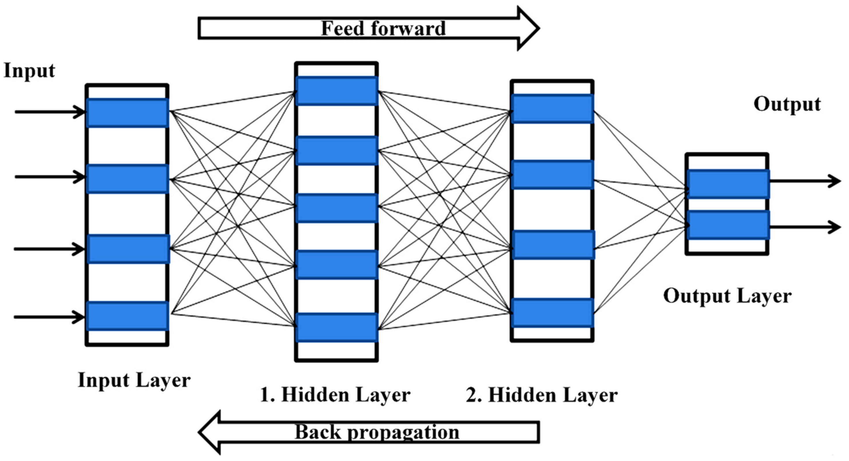
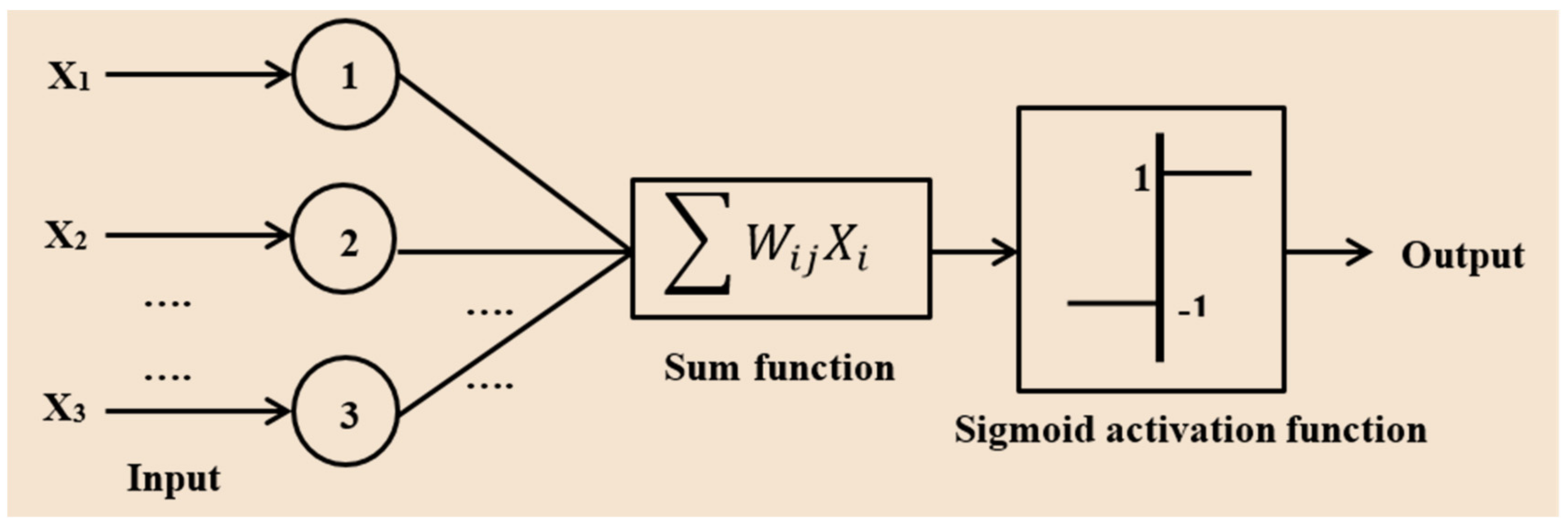
3.1.3. ANN Approach
3.1.4. Gradient Boosting Algorithm
- normal management of mixed form data,
- high predictive control,
- output space robustness (via robust loss functions)
- supports various loss functions.
3.2. Bagging and Bossing Approaches
Parameter Tuning for Ensemble Learner
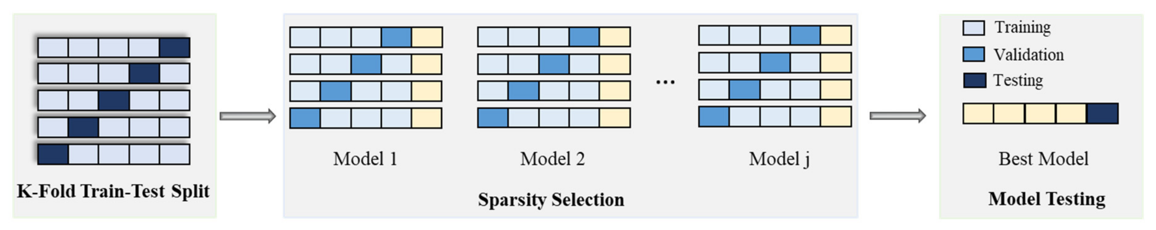
3.3. 10 K-Fold Cross-Validation Using 10 K-Fold Method
3.4. Evaluation of Models Using a Statistical Measure
4. Model Result
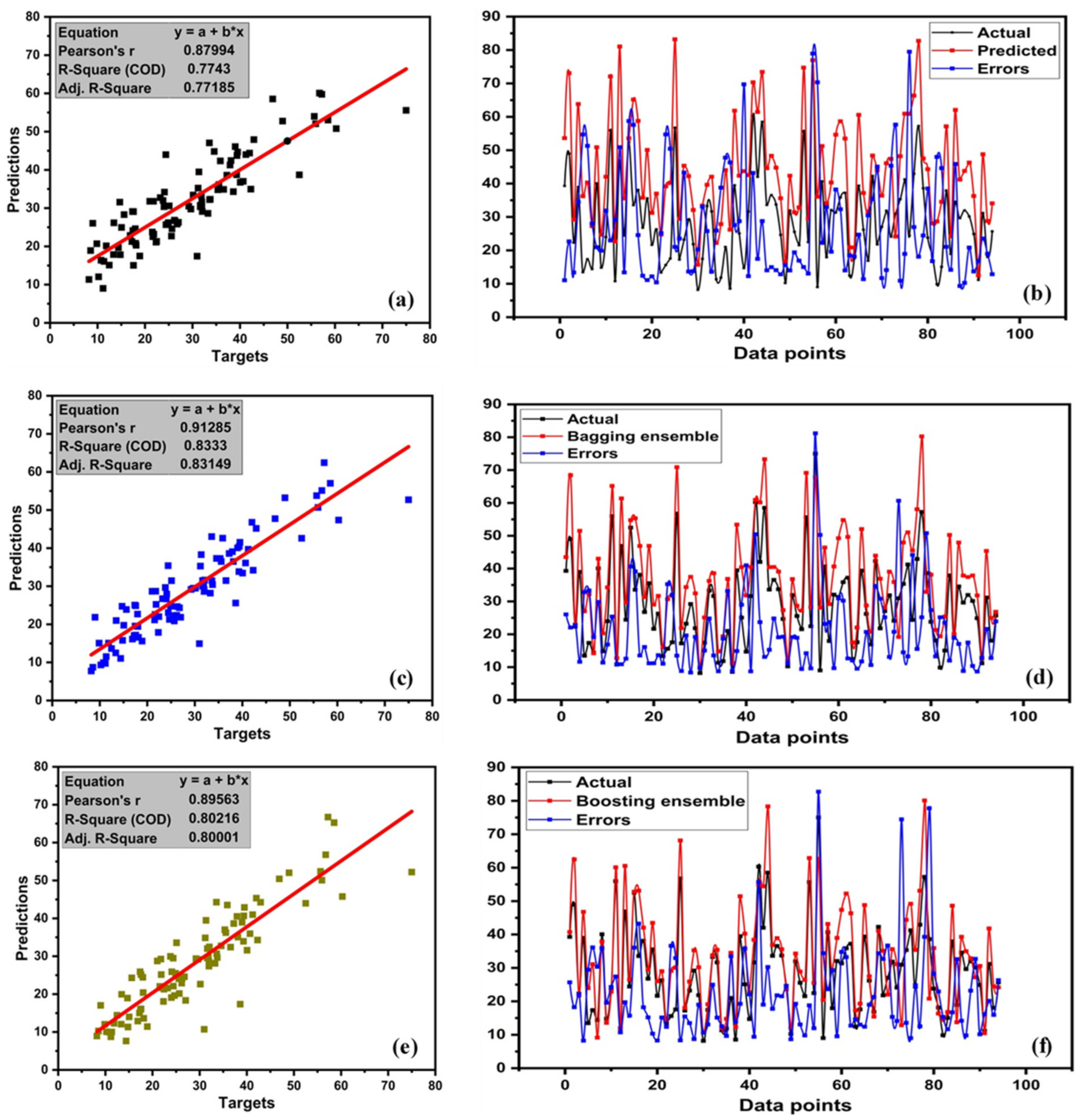
4.1. The Outcome of the DT Model
4.2. MLPNN Model Outcomes
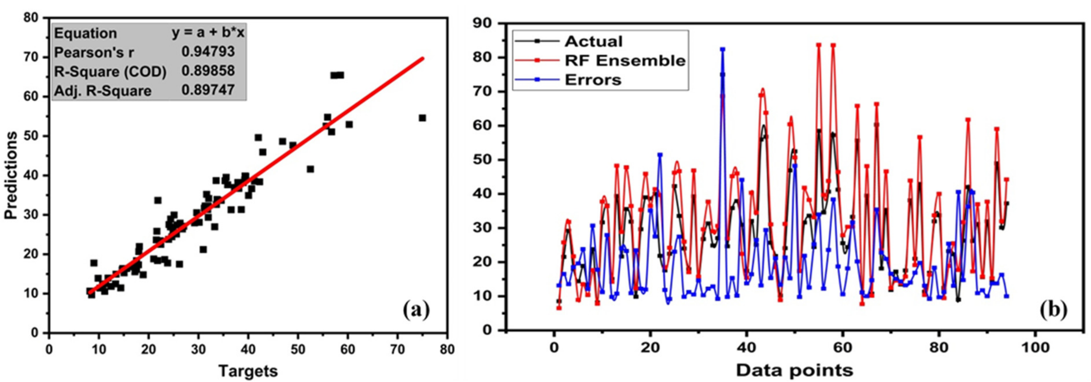
4.3. RF Model Outcome
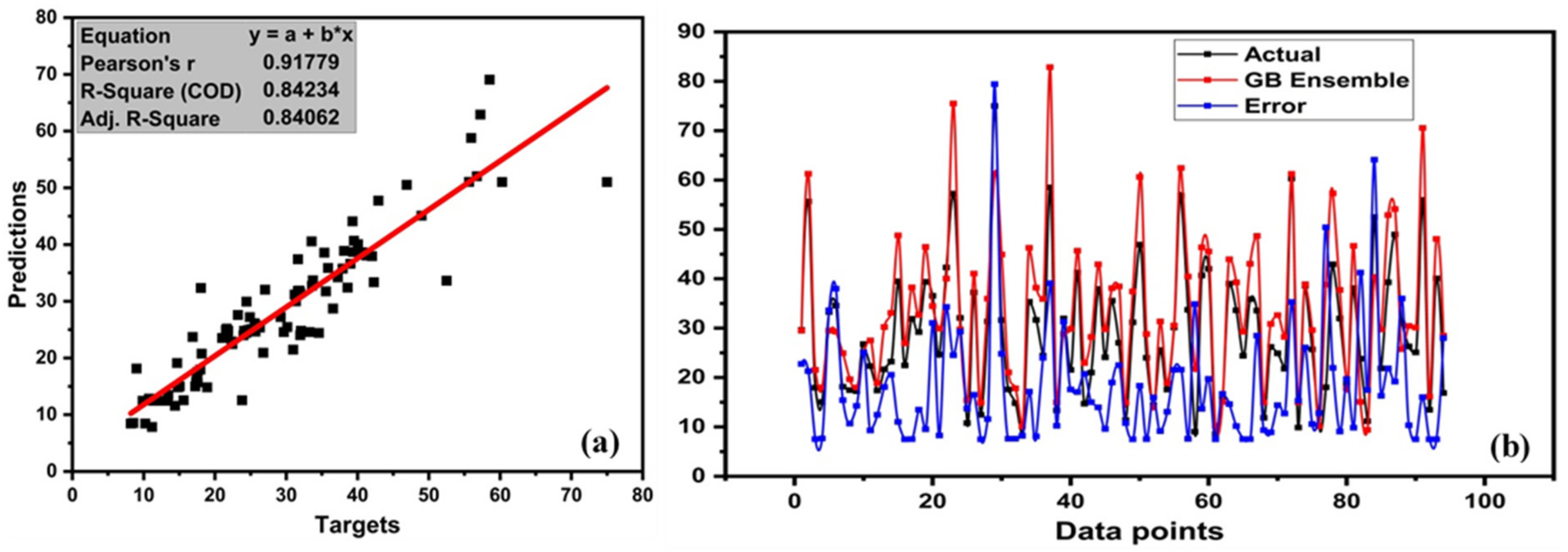
4.4. GB Model Outcome
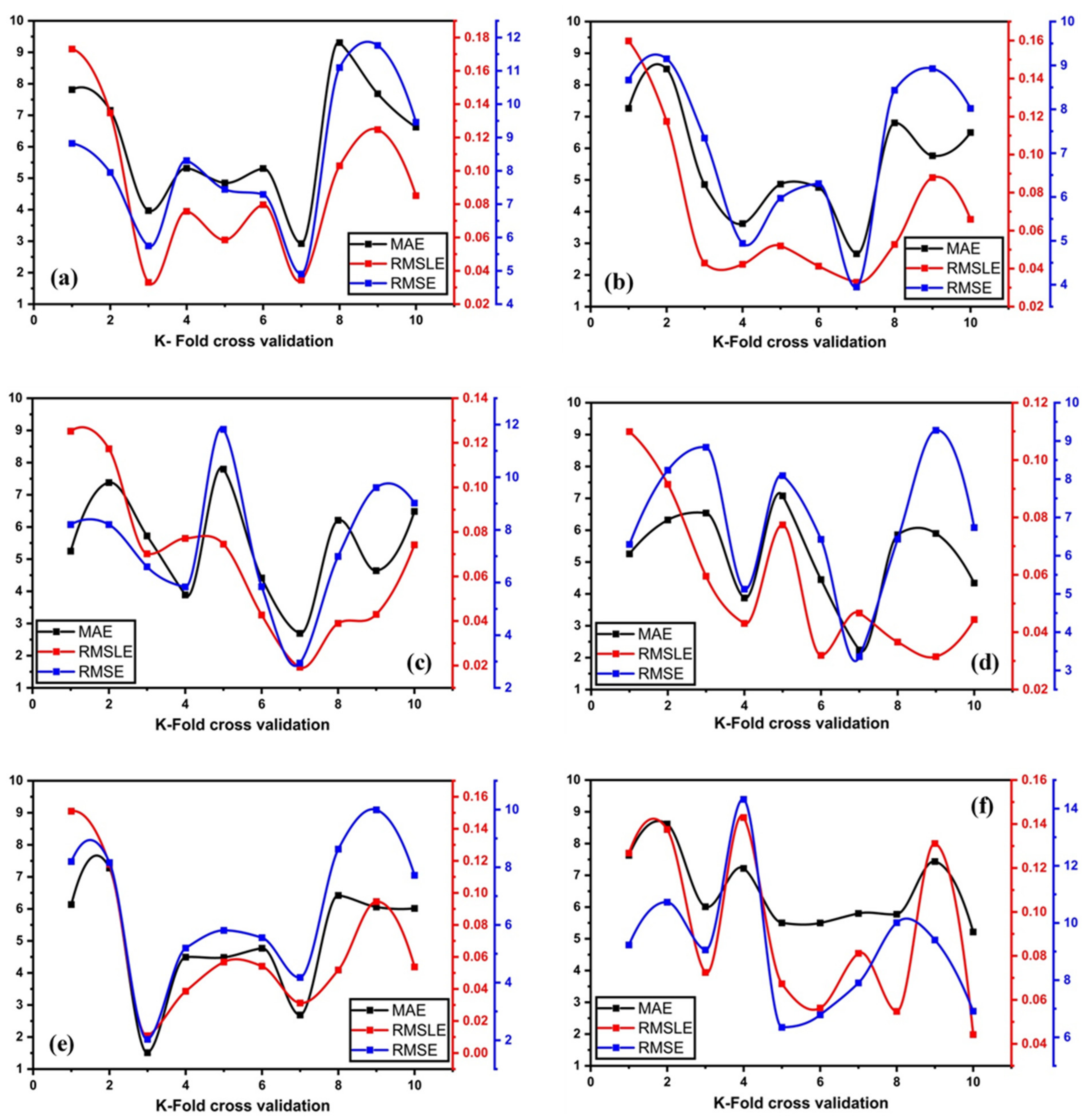
4.5. K-Fold Cross-Validation Approach
4.6. Results Evaluation of the Employed Models
5. Limitations and Future Work
6. Conclusions
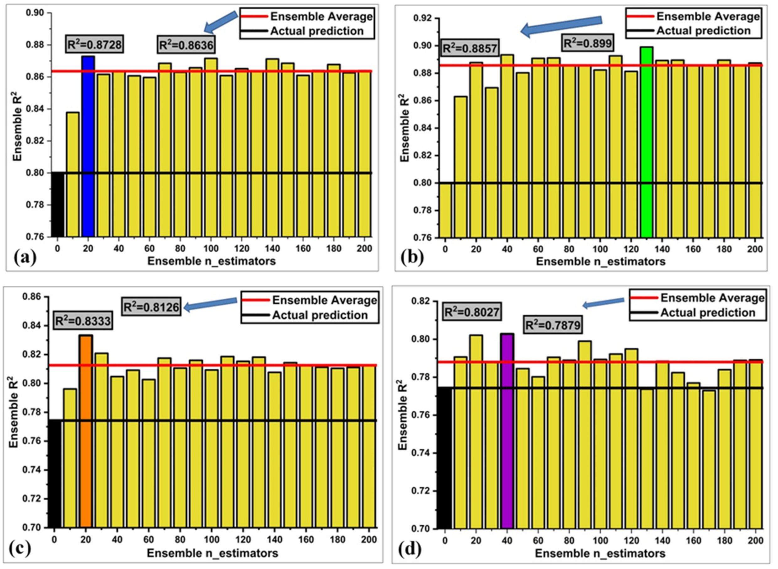
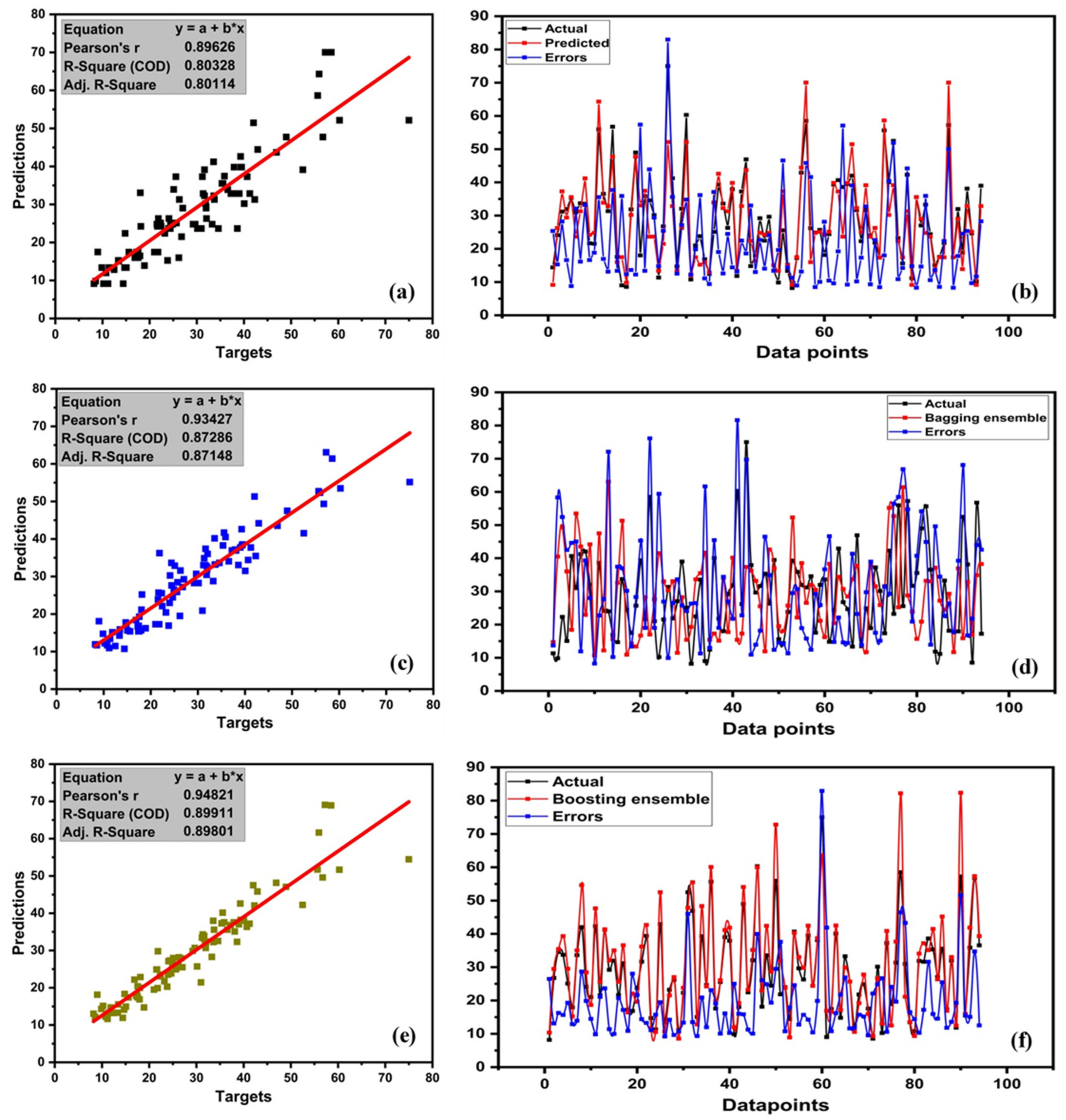
- The result of individual learners, DT and ANN, showed a strong correlation between predictions and targets with R2 = 0.80 and R2 = 0.77, respectively. However, ensemble learner with bagging and boosting and mostly boosting with Adaboost for DT outburst from the individual learner produced a stronger correlation R2 = 0.899, and ANN with bagging also produced a stronger correlation R2 = 0.833.
- Optimization of ensemble models was conducted with 20 models ranging from 10 to 200 estimators (sub-models). A decision tree with boosting (ensemble = 130) and random forest (ensemble = 130) provided a robust strong correlation with R2 = 0.89.
- It is evident that using ensemble learner with a weak learner showed less average error compared to the individual learner. Furthermore, K-fold cross-validation was used to validate models with coefficients of correlation, mean square error, and root mean square error. All the models had low MAE and RMSE errors and a high correlation R2. Fluctuations in validation were noticed, using K-fold validation to acquire data in steps and then performing validation on unknown data.
- Statistical analysis was also performed by means of MAE, MSE, RMSE, and MSLE. All ensemble learners produced less error compared to the individual learner, with random forest bagging giving a lesser error compared with MAE, MSE, RMSE, and MSLE. RF and AdaBoost are supervised learning algorithms that yielded strong relationships between prediction and targets.
Author Contributions
Funding
Institutional Review Board Statement
Informed Consent Statement
Data Availability Statement
Conflicts of Interest
Nomenclature
| HPC | High performance concrete |
| SRMs | Supplementary raw materials |
| GEP | Genetic engineering programming |
| GGBS | Ground granulated blast slag |
| GPC | Geopolymer concrete |
| GBA | Ground bottom ash |
| CFST | Concrete-filled steel tube |
| ANN | Artificial neuron network |
| ML | Machine learning |
| HPC | High-performance concrete |
| DL | Deep learning |
| DT | Decision tree |
| MLPNN | Multilayer perceptron neural network |
| DM | Deep machine |
| RF | Random forest |
| GB | Gradient boosting |
Appendix A
| S.No | Cement (kg/m3) | Fly Ash (kg/m3) | Water (kg/m3) | Superplasticizer (kg/m3) | Coarse Aggregate (kg/m3) | Fine Aggregate (kg/m3) | Age (Day) | Compressive Strength (MPa) |
| 1 | 540 | 0 | 162 | 2.5 | 1040 | 676 | 28 | 79.99 |
| 2 | 540 | 0 | 162 | 2.5 | 1055 | 676 | 28 | 61.89 |
| 3 | 475 | 0 | 228 | 0 | 932 | 594 | 28 | 39.29 |
| 4 | 380 | 0 | 228 | 0 | 932 | 670 | 90 | 52.91 |
| 5 | 475 | 0 | 228 | 0 | 932 | 594 | 180 | 42.62 |
| 6 | 380 | 0 | 228 | 0 | 932 | 670 | 365 | 52.52 |
| 7 | 380 | 0 | 228 | 0 | 932 | 670 | 270 | 53.3 |
| 8 | 475 | 0 | 228 | 0 | 932 | 594 | 7 | 38.6 |
| 9 | 475 | 0 | 228 | 0 | 932 | 594 | 270 | 42.13 |
| 10 | 475 | 0 | 228 | 0 | 932 | 594 | 90 | 42.23 |
| 11 | 380 | 0 | 228 | 0 | 932 | 670 | 180 | 53.1 |
| 12 | 349 | 0 | 192 | 0 | 1047 | 806.9 | 3 | 15.05 |
| 13 | 475 | 0 | 228 | 0 | 932 | 594 | 365 | 41.93 |
| 14 | 310 | 0 | 192 | 0 | 971 | 850.6 | 3 | 9.87 |
| 15 | 485 | 0 | 146 | 0 | 1120 | 800 | 28 | 71.99 |
| 16 | 531.3 | 0 | 141.8 | 28.2 | 852.1 | 893.7 | 3 | 41.3 |
| 17 | 531.3 | 0 | 141.8 | 28.2 | 852.1 | 893.7 | 7 | 46.9 |
| 18 | 531.3 | 0 | 141.8 | 28.2 | 852.1 | 893.7 | 28 | 56.4 |
| 19 | 531.3 | 0 | 141.8 | 28.2 | 852.1 | 893.7 | 56 | 58.8 |
| 20 | 531.3 | 0 | 141.8 | 28.2 | 852.1 | 893.7 | 91 | 59.2 |
| 21 | 222.4 | 96.7 | 189.3 | 4.5 | 967.1 | 870.3 | 3 | 11.58 |
| 22 | 222.4 | 96.7 | 189.3 | 4.5 | 967.1 | 870.3 | 14 | 24.45 |
| 23 | 222.4 | 96.7 | 189.3 | 4.5 | 967.1 | 870.3 | 28 | 24.89 |
| 24 | 222.4 | 96.7 | 189.3 | 4.5 | 967.1 | 870.3 | 56 | 29.45 |
| 25 | 222.4 | 96.7 | 189.3 | 4.5 | 967.1 | 870.3 | 100 | 40.71 |
| 26 | 233.8 | 94.6 | 197.9 | 4.6 | 947 | 852.2 | 3 | 10.38 |
| 27 | 233.8 | 94.6 | 197.9 | 4.6 | 947 | 852.2 | 14 | 22.14 |
| 28 | 233.8 | 94.6 | 197.9 | 4.6 | 947 | 852.2 | 28 | 22.84 |
| 29 | 233.8 | 94.6 | 197.9 | 4.6 | 947 | 852.2 | 56 | 27.66 |
| 30 | 233.8 | 94.6 | 197.9 | 4.6 | 947 | 852.2 | 100 | 34.56 |
| 31 | 194.7 | 100.5 | 165.6 | 7.5 | 1006.4 | 905.9 | 3 | 12.45 |
| 32 | 194.7 | 100.5 | 165.6 | 7.5 | 1006.4 | 905.9 | 14 | 24.99 |
| 33 | 194.7 | 100.5 | 165.6 | 7.5 | 1006.4 | 905.9 | 28 | 25.72 |
| 34 | 194.7 | 100.5 | 165.6 | 7.5 | 1006.4 | 905.9 | 56 | 33.96 |
| 35 | 194.7 | 100.5 | 165.6 | 7.5 | 1006.4 | 905.9 | 100 | 37.34 |
| 36 | 190.7 | 125.4 | 162.1 | 7.8 | 1090 | 804 | 3 | 15.04 |
| 37 | 190.7 | 125.4 | 162.1 | 7.8 | 1090 | 804 | 14 | 21.06 |
| 38 | 190.7 | 125.4 | 162.1 | 7.8 | 1090 | 804 | 28 | 26.4 |
| 39 | 190.7 | 125.4 | 162.1 | 7.8 | 1090 | 804 | 56 | 35.34 |
| 40 | 190.7 | 125.4 | 162.1 | 7.8 | 1090 | 804 | 100 | 40.57 |
| 41 | 212.1 | 121.6 | 180.3 | 5.7 | 1057.6 | 779.3 | 3 | 12.47 |
| 42 | 212.1 | 121.6 | 180.3 | 5.7 | 1057.6 | 779.3 | 14 | 20.92 |
| 43 | 212.1 | 121.6 | 180.3 | 5.7 | 1057.6 | 779.3 | 28 | 24.9 |
| 44 | 212.1 | 121.6 | 180.3 | 5.7 | 1057.6 | 779.3 | 56 | 34.2 |
| 45 | 212.1 | 121.6 | 180.3 | 5.7 | 1057.6 | 779.3 | 100 | 39.61 |
| 46 | 230 | 118.3 | 195.5 | 4.6 | 1029.4 | 758.6 | 3 | 10.03 |
| 47 | 230 | 118.3 | 195.5 | 4.6 | 1029.4 | 758.6 | 14 | 20.08 |
| 48 | 230 | 118.3 | 195.5 | 4.6 | 1029.4 | 758.6 | 28 | 24.48 |
| 49 | 230 | 118.3 | 195.5 | 4.6 | 1029.4 | 758.6 | 56 | 31.54 |
| 50 | 230 | 118.3 | 195.5 | 4.6 | 1029.4 | 758.6 | 100 | 35.34 |
| 51 | 190.3 | 125.2 | 161.9 | 9.9 | 1088.1 | 802.6 | 3 | 9.45 |
| 52 | 190.3 | 125.2 | 161.9 | 9.9 | 1088.1 | 802.6 | 14 | 22.72 |
| 53 | 190.3 | 125.2 | 161.9 | 9.9 | 1088.1 | 802.6 | 28 | 28.47 |
| 54 | 190.3 | 125.2 | 161.9 | 9.9 | 1088.1 | 802.6 | 56 | 38.56 |
| 55 | 190.3 | 125.2 | 161.9 | 9.9 | 1088.1 | 802.6 | 100 | 40.39 |
| 56 | 166.1 | 163.3 | 176.5 | 4.5 | 1058.6 | 780.1 | 3 | 10.76 |
| 57 | 166.1 | 163.3 | 176.5 | 4.5 | 1058.6 | 780.1 | 14 | 25.48 |
| 58 | 166.1 | 163.3 | 176.5 | 4.5 | 1058.6 | 780.1 | 28 | 21.54 |
| 59 | 166.1 | 163.3 | 176.5 | 4.5 | 1058.6 | 780.1 | 56 | 28.63 |
| 60 | 166.1 | 163.3 | 176.5 | 4.5 | 1058.6 | 780.1 | 100 | 33.54 |
| 61 | 229.7 | 118.2 | 195.2 | 6.1 | 1028.1 | 757.6 | 3 | 13.36 |
| 62 | 229.7 | 118.2 | 195.2 | 6.1 | 1028.1 | 757.6 | 14 | 22.32 |
| 63 | 229.7 | 118.2 | 195.2 | 6.1 | 1028.1 | 757.6 | 28 | 24.54 |
| 64 | 229.7 | 118.2 | 195.2 | 6.1 | 1028.1 | 757.6 | 56 | 31.35 |
| 65 | 229.7 | 118.2 | 195.2 | 6.1 | 1028.1 | 757.6 | 100 | 40.86 |
| 66 | 238.1 | 94.1 | 186.7 | 7 | 949.9 | 847 | 3 | 19.93 |
| 67 | 238.1 | 94.1 | 186.7 | 7 | 949.9 | 847 | 14 | 25.69 |
| 68 | 238.1 | 94.1 | 186.7 | 7 | 949.9 | 847 | 28 | 30.23 |
| 69 | 238.1 | 94.1 | 186.7 | 7 | 949.9 | 847 | 56 | 39.59 |
| 70 | 238.1 | 94.1 | 186.7 | 7 | 949.9 | 847 | 100 | 44.3 |
| 71 | 250 | 95.7 | 187.4 | 5.5 | 956.9 | 861.2 | 3 | 13.82 |
| 72 | 250 | 95.7 | 187.4 | 5.5 | 956.9 | 861.2 | 14 | 24.92 |
| 73 | 250 | 95.7 | 187.4 | 5.5 | 956.9 | 861.2 | 28 | 29.22 |
| 74 | 250 | 95.7 | 187.4 | 5.5 | 956.9 | 861.2 | 56 | 38.33 |
| 75 | 250 | 95.7 | 187.4 | 5.5 | 956.9 | 861.2 | 100 | 42.35 |
| 76 | 212.5 | 100.4 | 159.3 | 8.7 | 1007.8 | 903.6 | 3 | 13.54 |
| 77 | 212.5 | 100.4 | 159.3 | 8.7 | 1007.8 | 903.6 | 14 | 26.31 |
| 78 | 212.5 | 100.4 | 159.3 | 8.7 | 1007.8 | 903.6 | 28 | 31.64 |
| 79 | 212.5 | 100.4 | 159.3 | 8.7 | 1007.8 | 903.6 | 56 | 42.55 |
| 80 | 212.5 | 100.4 | 159.3 | 8.7 | 1007.8 | 903.6 | 100 | 42.92 |
| 81 | 212.6 | 100.4 | 159.4 | 10.4 | 1003.8 | 903.8 | 3 | 13.33 |
| 82 | 212.6 | 100.4 | 159.4 | 10.4 | 1003.8 | 903.8 | 14 | 25.37 |
| 83 | 212.6 | 100.4 | 159.4 | 10.4 | 1003.8 | 903.8 | 28 | 37.4 |
| 84 | 212.6 | 100.4 | 159.4 | 10.4 | 1003.8 | 903.8 | 56 | 44.4 |
| 85 | 212.6 | 100.4 | 159.4 | 10.4 | 1003.8 | 903.8 | 100 | 47.74 |
| 86 | 212 | 124.8 | 159 | 7.8 | 1085.4 | 799.5 | 3 | 19.52 |
| 87 | 212 | 124.8 | 159 | 7.8 | 1085.4 | 799.5 | 14 | 31.35 |
| 88 | 212 | 124.8 | 159 | 7.8 | 1085.4 | 799.5 | 28 | 38.5 |
| 89 | 212 | 124.8 | 159 | 7.8 | 1085.4 | 799.5 | 56 | 45.08 |
| 90 | 212 | 124.8 | 159 | 7.8 | 1085.4 | 799.5 | 100 | 47.82 |
| 91 | 231.8 | 121.6 | 174 | 6.7 | 1056.4 | 778.5 | 3 | 15.44 |
| 92 | 231.8 | 121.6 | 174 | 6.7 | 1056.4 | 778.5 | 14 | 26.77 |
| 93 | 231.8 | 121.6 | 174 | 6.7 | 1056.4 | 778.5 | 28 | 33.73 |
| 94 | 231.8 | 121.6 | 174 | 6.7 | 1056.4 | 778.5 | 56 | 42.7 |
| 95 | 231.8 | 121.6 | 174 | 6.7 | 1056.4 | 778.5 | 100 | 45.84 |
| 96 | 251.4 | 118.3 | 188.5 | 5.8 | 1028.4 | 757.7 | 3 | 17.22 |
| 97 | 251.4 | 118.3 | 188.5 | 5.8 | 1028.4 | 757.7 | 14 | 29.93 |
| 98 | 251.4 | 118.3 | 188.5 | 5.8 | 1028.4 | 757.7 | 28 | 29.65 |
| 99 | 251.4 | 118.3 | 188.5 | 5.8 | 1028.4 | 757.7 | 56 | 36.97 |
| 100 | 251.4 | 118.3 | 188.5 | 5.8 | 1028.4 | 757.7 | 100 | 43.58 |
| 101 | 251.4 | 118.3 | 188.5 | 6.4 | 1028.4 | 757.7 | 3 | 13.12 |
| 102 | 251.4 | 118.3 | 188.5 | 6.4 | 1028.4 | 757.7 | 14 | 24.43 |
| 103 | 251.4 | 118.3 | 188.5 | 6.4 | 1028.4 | 757.7 | 28 | 32.66 |
| 104 | 251.4 | 118.3 | 188.5 | 6.4 | 1028.4 | 757.7 | 56 | 36.64 |
| 105 | 251.4 | 118.3 | 188.5 | 6.4 | 1028.4 | 757.7 | 100 | 44.21 |
| 106 | 181.4 | 167 | 169.6 | 7.6 | 1055.6 | 777.8 | 3 | 13.62 |
| 107 | 181.4 | 167 | 169.6 | 7.6 | 1055.6 | 777.8 | 14 | 21.6 |
| 108 | 181.4 | 167 | 169.6 | 7.6 | 1055.6 | 777.8 | 28 | 27.77 |
| 109 | 181.4 | 167 | 169.6 | 7.6 | 1055.6 | 777.8 | 56 | 35.57 |
| 110 | 181.4 | 167 | 169.6 | 7.6 | 1055.6 | 777.8 | 100 | 45.37 |
| 111 | 290.4 | 96.2 | 168.1 | 9.4 | 961.2 | 865 | 3 | 22.5 |
| 112 | 290.4 | 96.2 | 168.1 | 9.4 | 961.2 | 865 | 14 | 34.67 |
| 113 | 290.4 | 96.2 | 168.1 | 9.4 | 961.2 | 865 | 28 | 34.74 |
| 114 | 290.4 | 96.2 | 168.1 | 9.4 | 961.2 | 865 | 56 | 45.08 |
| 115 | 290.4 | 96.2 | 168.1 | 9.4 | 961.2 | 865 | 100 | 48.97 |
| 116 | 277.1 | 97.4 | 160.6 | 11.8 | 973.9 | 875.6 | 3 | 23.14 |
| 117 | 277.1 | 97.4 | 160.6 | 11.8 | 973.9 | 875.6 | 14 | 41.89 |
| 118 | 277.1 | 97.4 | 160.6 | 11.8 | 973.9 | 875.6 | 28 | 48.28 |
| 119 | 277.1 | 97.4 | 160.6 | 11.8 | 973.9 | 875.6 | 56 | 51.04 |
| 120 | 277.1 | 97.4 | 160.6 | 11.8 | 973.9 | 875.6 | 100 | 55.64 |
| 121 | 295.7 | 95.6 | 171.5 | 8.9 | 955.1 | 859.2 | 3 | 22.95 |
| 122 | 295.7 | 95.6 | 171.5 | 8.9 | 955.1 | 859.2 | 14 | 35.23 |
| 123 | 295.7 | 95.6 | 171.5 | 8.9 | 955.1 | 859.2 | 28 | 39.94 |
| 124 | 295.7 | 95.6 | 171.5 | 8.9 | 955.1 | 859.2 | 56 | 48.72 |
| 125 | 295.7 | 95.6 | 171.5 | 8.9 | 955.1 | 859.2 | 100 | 52.04 |
| 126 | 251.8 | 99.9 | 146.1 | 12.4 | 1006 | 899.8 | 3 | 21.02 |
| 127 | 251.8 | 99.9 | 146.1 | 12.4 | 1006 | 899.8 | 14 | 33.36 |
| 128 | 251.8 | 99.9 | 146.1 | 12.4 | 1006 | 899.8 | 28 | 33.94 |
| 129 | 251.8 | 99.9 | 146.1 | 12.4 | 1006 | 899.8 | 56 | 44.14 |
| 130 | 251.8 | 99.9 | 146.1 | 12.4 | 1006 | 899.8 | 100 | 45.37 |
| 131 | 249.1 | 98.8 | 158.1 | 12.8 | 987.8 | 889 | 3 | 15.36 |
| 132 | 249.1 | 98.8 | 158.1 | 12.8 | 987.8 | 889 | 14 | 28.68 |
| 133 | 249.1 | 98.8 | 158.1 | 12.8 | 987.8 | 889 | 28 | 30.85 |
| 134 | 249.1 | 98.8 | 158.1 | 12.8 | 987.8 | 889 | 56 | 42.03 |
| 135 | 249.1 | 98.8 | 158.1 | 12.8 | 987.8 | 889 | 100 | 51.06 |
| 136 | 252.3 | 98.8 | 146.3 | 14.2 | 987.8 | 889 | 3 | 21.78 |
| 137 | 252.3 | 98.8 | 146.3 | 14.2 | 987.8 | 889 | 14 | 42.29 |
| 138 | 252.3 | 98.8 | 146.3 | 14.2 | 987.8 | 889 | 28 | 50.6 |
| 139 | 252.3 | 98.8 | 146.3 | 14.2 | 987.8 | 889 | 56 | 55.83 |
| 140 | 252.3 | 98.8 | 146.3 | 14.2 | 987.8 | 889 | 100 | 60.95 |
| 141 | 246.8 | 125.1 | 143.3 | 12 | 1086.8 | 800.9 | 3 | 23.52 |
| 142 | 246.8 | 125.1 | 143.3 | 12 | 1086.8 | 800.9 | 14 | 42.22 |
| 143 | 246.8 | 125.1 | 143.3 | 12 | 1086.8 | 800.9 | 28 | 52.5 |
| 144 | 246.8 | 125.1 | 143.3 | 12 | 1086.8 | 800.9 | 56 | 60.32 |
| 145 | 246.8 | 125.1 | 143.3 | 12 | 1086.8 | 800.9 | 100 | 66.42 |
| 146 | 275.1 | 121.4 | 159.5 | 9.9 | 1053.6 | 777.5 | 3 | 23.8 |
| 147 | 275.1 | 121.4 | 159.5 | 9.9 | 1053.6 | 777.5 | 14 | 38.77 |
| 148 | 275.1 | 121.4 | 159.5 | 9.9 | 1053.6 | 777.5 | 28 | 51.33 |
| 149 | 275.1 | 121.4 | 159.5 | 9.9 | 1053.6 | 777.5 | 56 | 56.85 |
| 150 | 275.1 | 121.4 | 159.5 | 9.9 | 1053.6 | 777.5 | 100 | 58.61 |
| 151 | 297.2 | 117.5 | 174.8 | 9.5 | 1022.8 | 753.5 | 3 | 21.91 |
| 152 | 297.2 | 117.5 | 174.8 | 9.5 | 1022.8 | 753.5 | 14 | 36.99 |
| 153 | 297.2 | 117.5 | 174.8 | 9.5 | 1022.8 | 753.5 | 28 | 47.4 |
| 154 | 297.2 | 117.5 | 174.8 | 9.5 | 1022.8 | 753.5 | 56 | 51.96 |
| 155 | 297.2 | 117.5 | 174.8 | 9.5 | 1022.8 | 753.5 | 100 | 56.74 |
| 156 | 213.7 | 174.7 | 154.8 | 10.2 | 1053.5 | 776.4 | 3 | 17.57 |
| 157 | 213.7 | 174.7 | 154.8 | 10.2 | 1053.5 | 776.4 | 14 | 33.73 |
| 158 | 213.7 | 174.7 | 154.8 | 10.2 | 1053.5 | 776.4 | 28 | 40.15 |
| 159 | 213.7 | 174.7 | 154.8 | 10.2 | 1053.5 | 776.4 | 56 | 46.64 |
| 160 | 213.7 | 174.7 | 154.8 | 10.2 | 1053.5 | 776.4 | 100 | 50.08 |
| 161 | 213.5 | 174.2 | 154.6 | 11.7 | 1052.3 | 775.5 | 3 | 17.37 |
| 162 | 213.5 | 174.2 | 154.6 | 11.7 | 1052.3 | 775.5 | 14 | 33.7 |
| 163 | 213.5 | 174.2 | 154.6 | 11.7 | 1052.3 | 775.5 | 28 | 45.94 |
| 164 | 213.5 | 174.2 | 154.6 | 11.7 | 1052.3 | 775.5 | 56 | 51.43 |
| 165 | 213.5 | 174.2 | 154.6 | 11.7 | 1052.3 | 775.5 | 100 | 59.3 |
| 166 | 218.9 | 124.1 | 158.5 | 11.3 | 1078.7 | 794.9 | 3 | 15.34 |
| 167 | 218.9 | 124.1 | 158.5 | 11.3 | 1078.7 | 794.9 | 14 | 26.05 |
| 168 | 218.9 | 124.1 | 158.5 | 11.3 | 1078.7 | 794.9 | 28 | 30.22 |
| 169 | 218.9 | 124.1 | 158.5 | 11.3 | 1078.7 | 794.9 | 56 | 37.27 |
| 170 | 218.9 | 124.1 | 158.5 | 11.3 | 1078.7 | 794.9 | 100 | 46.23 |
| 171 | 376 | 0 | 214.6 | 0 | 1003.5 | 762.4 | 3 | 16.28 |
| 172 | 376 | 0 | 214.6 | 0 | 1003.5 | 762.4 | 14 | 25.62 |
| 173 | 376 | 0 | 214.6 | 0 | 1003.5 | 762.4 | 28 | 31.97 |
| 174 | 376 | 0 | 214.6 | 0 | 1003.5 | 762.4 | 56 | 36.3 |
| 175 | 376 | 0 | 214.6 | 0 | 1003.5 | 762.4 | 100 | 43.06 |
| 176 | 500 | 0 | 140 | 4 | 966 | 853 | 28 | 67.57 |
| 177 | 475 | 59 | 142 | 1.9 | 1098 | 641 | 28 | 57.23 |
| 178 | 505 | 60 | 195 | 0 | 1030 | 630 | 28 | 64.02 |
| 179 | 451 | 0 | 165 | 11.3 | 1030 | 745 | 28 | 78.8 |
| 180 | 516 | 0 | 162 | 8.2 | 801 | 802 | 28 | 41.37 |
| 181 | 520 | 0 | 170 | 5.2 | 855 | 855 | 28 | 60.28 |
| 182 | 528 | 0 | 185 | 6.9 | 920 | 720 | 28 | 56.83 |
| 183 | 520 | 0 | 175 | 5.2 | 870 | 805 | 28 | 51.02 |
| 184 | 385 | 136 | 158 | 20 | 903 | 768 | 28 | 55.55 |
| 185 | 500.1 | 0 | 200 | 3 | 1124.4 | 613.2 | 28 | 44.13 |
| 186 | 405 | 0 | 175 | 0 | 1120 | 695 | 28 | 52.3 |
| 187 | 516 | 0 | 162 | 8.3 | 801 | 802 | 28 | 41.37 |
| 188 | 475 | 0 | 162 | 9.5 | 1044 | 662 | 28 | 58.52 |
| 189 | 500 | 0 | 151 | 9 | 1033 | 655 | 28 | 69.84 |
| 190 | 165 | 143.6 | 163.8 | 0 | 1005.6 | 900.9 | 3 | 14.4 |
| 191 | 190.3 | 125.2 | 166.6 | 9.9 | 1079 | 798.9 | 3 | 12.55 |
| 192 | 250 | 95.7 | 191.8 | 5.3 | 948.9 | 857.2 | 3 | 8.49 |
| 193 | 213.5 | 174.2 | 159.2 | 11.7 | 1043.6 | 771.9 | 3 | 15.61 |
| 194 | 194.7 | 100.5 | 170.2 | 7.5 | 998 | 901.8 | 3 | 12.18 |
| 195 | 251.4 | 118.3 | 192.9 | 5.8 | 1043.6 | 754.3 | 3 | 11.98 |
| 196 | 165 | 143.6 | 163.8 | 0 | 1005.6 | 900.9 | 14 | 16.88 |
| 197 | 190.3 | 125.2 | 166.6 | 9.9 | 1079 | 798.9 | 14 | 19.42 |
| 198 | 250 | 95.7 | 191.8 | 5.3 | 948.9 | 857.2 | 14 | 24.66 |
| 199 | 213.5 | 174.2 | 159.2 | 11.7 | 1043.6 | 771.9 | 14 | 29.59 |
| 200 | 194.7 | 100.5 | 170.2 | 7.5 | 998 | 901.8 | 14 | 24.28 |
| 201 | 251.4 | 118.3 | 192.9 | 5.8 | 1043.6 | 754.3 | 14 | 20.73 |
| 202 | 165 | 143.6 | 163.8 | 0 | 1005.6 | 900.9 | 28 | 26.2 |
| 203 | 190.3 | 125.2 | 166.6 | 9.9 | 1079 | 798.9 | 28 | 24.85 |
| 204 | 250 | 95.7 | 191.8 | 5.3 | 948.9 | 857.2 | 28 | 27.22 |
| 205 | 213.5 | 174.2 | 159.2 | 11.7 | 1043.6 | 771.9 | 28 | 44.64 |
| 206 | 194.7 | 100.5 | 170.2 | 7.5 | 998 | 901.8 | 28 | 37.27 |
| 207 | 251.4 | 118.3 | 192.9 | 5.8 | 1043.6 | 754.3 | 28 | 33.27 |
| 208 | 165 | 143.6 | 163.8 | 0 | 1005.6 | 900.9 | 56 | 36.56 |
| 209 | 190.3 | 125.2 | 166.6 | 9.9 | 1079 | 798.9 | 56 | 31.72 |
| 210 | 250 | 95.7 | 191.8 | 5.3 | 948.9 | 857.2 | 56 | 39.64 |
| 211 | 213.5 | 174.2 | 159.2 | 11.7 | 1043.6 | 771.9 | 56 | 51.26 |
| 212 | 194.7 | 100.5 | 170.2 | 7.5 | 998 | 901.8 | 56 | 43.39 |
| 213 | 251.4 | 118.3 | 192.9 | 5.8 | 1043.6 | 754.3 | 56 | 39.27 |
| 214 | 165 | 143.6 | 163.8 | 0 | 1005.6 | 900.9 | 100 | 37.96 |
| 215 | 190.3 | 125.2 | 166.6 | 9.9 | 1079 | 798.9 | 100 | 33.56 |
| 216 | 250 | 95.7 | 191.8 | 5.3 | 948.9 | 857.2 | 100 | 41.16 |
| 217 | 213.5 | 174.2 | 159.2 | 11.7 | 1043.6 | 771.9 | 100 | 52.96 |
| 218 | 194.7 | 100.5 | 170.2 | 7.5 | 998 | 901.8 | 100 | 44.28 |
| 219 | 251.4 | 118.3 | 192.9 | 5.8 | 1043.6 | 754.3 | 100 | 40.15 |
| 220 | 436 | 0 | 218 | 0 | 838.4 | 719.7 | 28 | 23.85 |
| 221 | 289 | 0 | 192 | 0 | 913.2 | 895.3 | 90 | 32.07 |
| 222 | 289 | 0 | 192 | 0 | 913.2 | 895.3 | 3 | 11.65 |
| 223 | 393 | 0 | 192 | 0 | 940.6 | 785.6 | 3 | 19.2 |
| 224 | 393 | 0 | 192 | 0 | 940.6 | 785.6 | 90 | 48.85 |
| 225 | 393 | 0 | 192 | 0 | 940.6 | 785.6 | 28 | 39.6 |
| 226 | 480 | 0 | 192 | 0 | 936.2 | 712.2 | 28 | 43.94 |
| 227 | 480 | 0 | 192 | 0 | 936.2 | 712.2 | 7 | 34.57 |
| 228 | 480 | 0 | 192 | 0 | 936.2 | 712.2 | 90 | 54.32 |
| 229 | 480 | 0 | 192 | 0 | 936.2 | 712.2 | 3 | 24.4 |
| 230 | 333 | 0 | 192 | 0 | 931.2 | 842.6 | 3 | 15.62 |
| 231 | 255 | 0 | 192 | 0 | 889.8 | 945 | 90 | 21.86 |
| 232 | 255 | 0 | 192 | 0 | 889.8 | 945 | 7 | 10.22 |
| 233 | 289 | 0 | 192 | 0 | 913.2 | 895.3 | 7 | 14.6 |
| 234 | 255 | 0 | 192 | 0 | 889.8 | 945 | 28 | 18.75 |
| 235 | 333 | 0 | 192 | 0 | 931.2 | 842.6 | 28 | 31.97 |
| 236 | 333 | 0 | 192 | 0 | 931.2 | 842.6 | 7 | 23.4 |
| 237 | 289 | 0 | 192 | 0 | 913.2 | 895.3 | 28 | 25.57 |
| 238 | 333 | 0 | 192 | 0 | 931.2 | 842.6 | 90 | 41.68 |
| 239 | 393 | 0 | 192 | 0 | 940.6 | 785.6 | 7 | 27.74 |
| 240 | 255 | 0 | 192 | 0 | 889.8 | 945 | 3 | 8.2 |
| 241 | 397 | 0 | 185.7 | 0 | 1040.6 | 734.3 | 28 | 33.08 |
| 242 | 382.5 | 0 | 185.7 | 0 | 1047.8 | 739.3 | 7 | 24.07 |
| 243 | 295.8 | 0 | 185.7 | 0 | 1091.4 | 769.3 | 7 | 14.84 |
| 244 | 397 | 0 | 185.7 | 0 | 1040.6 | 734.3 | 7 | 25.45 |
| 245 | 381.4 | 0 | 185.7 | 0 | 1104.6 | 784.3 | 28 | 22.49 |
| 246 | 295.8 | 0 | 185.7 | 0 | 1091.4 | 769.3 | 28 | 25.22 |
| 247 | 238.1 | 0 | 185.7 | 0 | 1118.8 | 789.3 | 28 | 17.58 |
| 248 | 339.2 | 0 | 185.7 | 0 | 1069.2 | 754.3 | 7 | 21.18 |
| 249 | 381.4 | 0 | 185.7 | 0 | 1104.6 | 784.3 | 7 | 14.54 |
| 250 | 339.2 | 0 | 185.7 | 0 | 1069.2 | 754.3 | 28 | 31.9 |
| 251 | 238.1 | 0 | 185.7 | 0 | 1118.8 | 789.3 | 7 | 10.34 |
| 252 | 252.5 | 0 | 185.7 | 0 | 1111.6 | 784.3 | 28 | 19.77 |
| 253 | 382.5 | 0 | 185.7 | 0 | 1047.8 | 739.3 | 28 | 37.44 |
| 254 | 252.5 | 0 | 185.7 | 0 | 1111.6 | 784.3 | 7 | 11.48 |
| 255 | 339 | 0 | 197 | 0 | 968 | 781 | 3 | 13.22 |
| 256 | 339 | 0 | 197 | 0 | 968 | 781 | 7 | 20.97 |
| 257 | 339 | 0 | 197 | 0 | 968 | 781 | 14 | 27.04 |
| 258 | 339 | 0 | 197 | 0 | 968 | 781 | 28 | 32.04 |
| 259 | 339 | 0 | 197 | 0 | 968 | 781 | 90 | 35.17 |
| 260 | 339 | 0 | 197 | 0 | 968 | 781 | 180 | 36.45 |
| 261 | 339 | 0 | 197 | 0 | 968 | 781 | 365 | 38.89 |
| 262 | 236 | 0 | 194 | 0 | 968 | 885 | 3 | 6.47 |
| 263 | 236 | 0 | 194 | 0 | 968 | 885 | 14 | 12.84 |
| 264 | 236 | 0 | 194 | 0 | 968 | 885 | 28 | 18.42 |
| 265 | 236 | 0 | 194 | 0 | 968 | 885 | 90 | 21.95 |
| 266 | 236 | 0 | 193 | 0 | 968 | 885 | 180 | 24.1 |
| 267 | 236 | 0 | 193 | 0 | 968 | 885 | 365 | 25.08 |
| 268 | 277 | 0 | 191 | 0 | 968 | 856 | 14 | 21.26 |
| 269 | 277 | 0 | 191 | 0 | 968 | 856 | 28 | 25.97 |
| 270 | 277 | 0 | 191 | 0 | 968 | 856 | 3 | 11.36 |
| 271 | 277 | 0 | 191 | 0 | 968 | 856 | 90 | 31.25 |
| 272 | 277 | 0 | 191 | 0 | 968 | 856 | 180 | 32.33 |
| 273 | 277 | 0 | 191 | 0 | 968 | 856 | 360 | 33.7 |
| 274 | 254 | 0 | 198 | 0 | 968 | 863 | 3 | 9.31 |
| 275 | 254 | 0 | 198 | 0 | 968 | 863 | 90 | 26.94 |
| 276 | 254 | 0 | 198 | 0 | 968 | 863 | 180 | 27.63 |
| 277 | 254 | 0 | 198 | 0 | 968 | 863 | 365 | 29.79 |
| 278 | 307 | 0 | 193 | 0 | 968 | 812 | 180 | 34.49 |
| 279 | 307 | 0 | 193 | 0 | 968 | 812 | 365 | 36.15 |
| 280 | 307 | 0 | 193 | 0 | 968 | 812 | 3 | 12.54 |
| 281 | 307 | 0 | 193 | 0 | 968 | 812 | 28 | 27.53 |
| 282 | 307 | 0 | 193 | 0 | 968 | 812 | 90 | 32.92 |
| 283 | 236 | 0 | 193 | 0 | 968 | 885 | 7 | 9.99 |
| 284 | 200 | 0 | 180 | 0 | 1125 | 845 | 7 | 7.84 |
| 285 | 200 | 0 | 180 | 0 | 1125 | 845 | 28 | 12.25 |
| 286 | 225 | 0 | 181 | 0 | 1113 | 833 | 7 | 11.17 |
| 287 | 225 | 0 | 181 | 0 | 1113 | 833 | 28 | 17.34 |
| 288 | 325 | 0 | 184 | 0 | 1063 | 783 | 7 | 17.54 |
| 289 | 325 | 0 | 184 | 0 | 1063 | 783 | 28 | 30.57 |
| 290 | 275 | 0 | 183 | 0 | 1088 | 808 | 7 | 14.2 |
| 291 | 275 | 0 | 183 | 0 | 1088 | 808 | 28 | 24.5 |
| 292 | 300 | 0 | 184 | 0 | 1075 | 795 | 7 | 15.58 |
| 293 | 300 | 0 | 184 | 0 | 1075 | 795 | 28 | 26.85 |
| 294 | 375 | 0 | 186 | 0 | 1038 | 758 | 7 | 26.06 |
| 295 | 375 | 0 | 186 | 0 | 1038 | 758 | 28 | 38.21 |
| 296 | 400 | 0 | 187 | 0 | 1025 | 745 | 28 | 43.7 |
| 297 | 400 | 0 | 187 | 0 | 1025 | 745 | 7 | 30.14 |
| 298 | 250 | 0 | 182 | 0 | 1100 | 820 | 7 | 12.73 |
| 299 | 250 | 0 | 182 | 0 | 1100 | 820 | 28 | 20.87 |
| 300 | 350 | 0 | 186 | 0 | 1050 | 770 | 7 | 20.28 |
| 301 | 350 | 0 | 186 | 0 | 1050 | 770 | 28 | 34.29 |
| 302 | 310 | 0 | 192 | 0 | 1012 | 830 | 3 | 11.85 |
| 303 | 310 | 0 | 192 | 0 | 1012 | 830 | 7 | 17.24 |
| 304 | 310 | 0 | 192 | 0 | 1012 | 830 | 28 | 27.83 |
| 305 | 310 | 0 | 192 | 0 | 1012 | 830 | 90 | 35.76 |
| 306 | 310 | 0 | 192 | 0 | 1012 | 830 | 120 | 38.7 |
| 307 | 331 | 0 | 192 | 0 | 1025 | 821 | 3 | 14.31 |
| 308 | 331 | 0 | 192 | 0 | 1025 | 821 | 7 | 17.44 |
| 309 | 331 | 0 | 192 | 0 | 1025 | 821 | 28 | 31.74 |
| 310 | 331 | 0 | 192 | 0 | 1025 | 821 | 90 | 37.91 |
| 311 | 331 | 0 | 192 | 0 | 1025 | 821 | 120 | 39.38 |
| 312 | 349 | 0 | 192 | 0 | 1056 | 809 | 3 | 15.87 |
| 313 | 349 | 0 | 192 | 0 | 1056 | 809 | 7 | 9.01 |
| 314 | 349 | 0 | 192 | 0 | 1056 | 809 | 28 | 33.61 |
| 315 | 349 | 0 | 192 | 0 | 1056 | 809 | 90 | 40.66 |
| 316 | 349 | 0 | 192 | 0 | 1056 | 809 | 120 | 40.86 |
| 317 | 238 | 0 | 186 | 0 | 1119 | 789 | 7 | 12.05 |
| 318 | 238 | 0 | 186 | 0 | 1119 | 789 | 28 | 17.54 |
| 319 | 296 | 0 | 186 | 0 | 1090 | 769 | 7 | 18.91 |
| 320 | 296 | 0 | 186 | 0 | 1090 | 769 | 28 | 25.18 |
| 321 | 297 | 0 | 186 | 0 | 1040 | 734 | 7 | 30.96 |
| 322 | 480 | 0 | 192 | 0 | 936 | 721 | 28 | 43.89 |
| 323 | 480 | 0 | 192 | 0 | 936 | 721 | 90 | 54.28 |
| 324 | 397 | 0 | 186 | 0 | 1040 | 734 | 28 | 36.94 |
| 325 | 281 | 0 | 186 | 0 | 1104 | 774 | 7 | 14.5 |
| 326 | 281 | 0 | 185 | 0 | 1104 | 774 | 28 | 22.44 |
| 327 | 500 | 0 | 200 | 0 | 1125 | 613 | 1 | 12.64 |
| 328 | 500 | 0 | 200 | 0 | 1125 | 613 | 3 | 26.06 |
| 329 | 500 | 0 | 200 | 0 | 1125 | 613 | 7 | 33.21 |
| 330 | 500 | 0 | 200 | 0 | 1125 | 613 | 14 | 36.94 |
| 331 | 500 | 0 | 200 | 0 | 1125 | 613 | 28 | 44.09 |
| 332 | 540 | 0 | 173 | 0 | 1125 | 613 | 7 | 52.61 |
| 333 | 540 | 0 | 173 | 0 | 1125 | 613 | 14 | 59.76 |
| 334 | 540 | 0 | 173 | 0 | 1125 | 613 | 28 | 67.31 |
| 335 | 540 | 0 | 173 | 0 | 1125 | 613 | 90 | 69.66 |
| 336 | 540 | 0 | 173 | 0 | 1125 | 613 | 180 | 71.62 |
| 337 | 540 | 0 | 173 | 0 | 1125 | 613 | 270 | 74.17 |
| 338 | 350 | 0 | 203 | 0 | 974 | 775 | 7 | 18.13 |
| 339 | 350 | 0 | 203 | 0 | 974 | 775 | 14 | 22.53 |
| 340 | 350 | 0 | 203 | 0 | 974 | 775 | 28 | 27.34 |
| 341 | 350 | 0 | 203 | 0 | 974 | 775 | 56 | 29.98 |
| 342 | 350 | 0 | 203 | 0 | 974 | 775 | 90 | 31.35 |
| 343 | 350 | 0 | 203 | 0 | 974 | 775 | 180 | 32.72 |
| 344 | 385 | 0 | 186 | 0 | 966 | 763 | 1 | 6.27 |
| 345 | 385 | 0 | 186 | 0 | 966 | 763 | 3 | 14.7 |
| 346 | 385 | 0 | 186 | 0 | 966 | 763 | 7 | 23.22 |
| 347 | 385 | 0 | 186 | 0 | 966 | 763 | 14 | 27.92 |
| 348 | 385 | 0 | 186 | 0 | 966 | 763 | 28 | 31.35 |
| 349 | 331 | 0 | 192 | 0 | 978 | 825 | 180 | 39 |
| 350 | 331 | 0 | 192 | 0 | 978 | 825 | 360 | 41.24 |
| 351 | 349 | 0 | 192 | 0 | 1047 | 806 | 3 | 14.99 |
| 352 | 331 | 0 | 192 | 0 | 978 | 825 | 3 | 13.52 |
| 353 | 382 | 0 | 186 | 0 | 1047 | 739 | 7 | 24 |
| 354 | 382 | 0 | 186 | 0 | 1047 | 739 | 28 | 37.42 |
| 355 | 382 | 0 | 186 | 0 | 1111 | 784 | 7 | 11.47 |
| 356 | 281 | 0 | 186 | 0 | 1104 | 774 | 28 | 22.44 |
| 357 | 339 | 0 | 185 | 0 | 1069 | 754 | 7 | 21.16 |
| 358 | 339 | 0 | 185 | 0 | 1069 | 754 | 28 | 31.84 |
| 359 | 295 | 0 | 185 | 0 | 1069 | 769 | 7 | 14.8 |
| 360 | 295 | 0 | 185 | 0 | 1069 | 769 | 28 | 25.18 |
| 361 | 238 | 0 | 185 | 0 | 1118 | 789 | 28 | 17.54 |
| 362 | 296 | 0 | 192 | 0 | 1085 | 765 | 7 | 14.2 |
| 363 | 296 | 0 | 192 | 0 | 1085 | 765 | 28 | 21.65 |
| 364 | 296 | 0 | 192 | 0 | 1085 | 765 | 90 | 29.39 |
| 365 | 331 | 0 | 192 | 0 | 879 | 825 | 3 | 13.52 |
| 366 | 331 | 0 | 192 | 0 | 978 | 825 | 7 | 16.26 |
| 367 | 331 | 0 | 192 | 0 | 978 | 825 | 28 | 31.45 |
| 368 | 331 | 0 | 192 | 0 | 978 | 825 | 90 | 37.23 |
| 369 | 349 | 0 | 192 | 0 | 1047 | 806 | 7 | 18.13 |
| 370 | 349 | 0 | 192 | 0 | 1047 | 806 | 28 | 32.72 |
| 371 | 349 | 0 | 192 | 0 | 1047 | 806 | 90 | 39.49 |
| 372 | 349 | 0 | 192 | 0 | 1047 | 806 | 180 | 41.05 |
| 373 | 349 | 0 | 192 | 0 | 1047 | 806 | 360 | 42.13 |
| 374 | 302 | 0 | 203 | 0 | 974 | 817 | 14 | 18.13 |
| 375 | 302 | 0 | 203 | 0 | 974 | 817 | 180 | 26.74 |
| 376 | 525 | 0 | 189 | 0 | 1125 | 613 | 180 | 61.92 |
| 377 | 500 | 0 | 200 | 0 | 1125 | 613 | 90 | 47.22 |
| 378 | 500 | 0 | 200 | 0 | 1125 | 613 | 180 | 51.04 |
| 379 | 500 | 0 | 200 | 0 | 1125 | 613 | 270 | 55.16 |
| 380 | 540 | 0 | 173 | 0 | 1125 | 613 | 3 | 41.64 |
| 381 | 252 | 0 | 185 | 0 | 1111 | 784 | 7 | 13.71 |
| 382 | 252 | 0 | 185 | 0 | 1111 | 784 | 28 | 19.69 |
| 383 | 339 | 0 | 185 | 0 | 1060 | 754 | 28 | 31.65 |
| 384 | 393 | 0 | 192 | 0 | 940 | 758 | 3 | 19.11 |
| 385 | 393 | 0 | 192 | 0 | 940 | 758 | 28 | 39.58 |
| 386 | 393 | 0 | 192 | 0 | 940 | 758 | 90 | 48.79 |
| 387 | 382 | 0 | 185 | 0 | 1047 | 739 | 7 | 24 |
| 388 | 382 | 0 | 185 | 0 | 1047 | 739 | 28 | 37.42 |
| 389 | 252 | 0 | 186 | 0 | 1111 | 784 | 7 | 11.47 |
| 390 | 252 | 0 | 185 | 0 | 1111 | 784 | 28 | 19.69 |
| 391 | 310 | 0 | 192 | 0 | 970 | 850 | 7 | 14.99 |
| 392 | 310 | 0 | 192 | 0 | 970 | 850 | 28 | 27.92 |
| 393 | 310 | 0 | 192 | 0 | 970 | 850 | 90 | 34.68 |
| 394 | 310 | 0 | 192 | 0 | 970 | 850 | 180 | 37.33 |
| 395 | 310 | 0 | 192 | 0 | 970 | 850 | 360 | 38.11 |
| 396 | 525 | 0 | 189 | 0 | 1125 | 613 | 3 | 33.8 |
| 397 | 525 | 0 | 189 | 0 | 1125 | 613 | 7 | 42.42 |
| 398 | 525 | 0 | 189 | 0 | 1125 | 613 | 14 | 48.4 |
| 399 | 525 | 0 | 189 | 0 | 1125 | 613 | 28 | 55.94 |
| 400 | 525 | 0 | 189 | 0 | 1125 | 613 | 90 | 58.78 |
| 401 | 525 | 0 | 189 | 0 | 1125 | 613 | 270 | 67.11 |
| 402 | 322 | 0 | 203 | 0 | 974 | 800 | 14 | 20.77 |
| 403 | 322 | 0 | 203 | 0 | 974 | 800 | 28 | 25.18 |
| 404 | 322 | 0 | 203 | 0 | 974 | 800 | 180 | 29.59 |
| 405 | 302 | 0 | 203 | 0 | 974 | 817 | 28 | 21.75 |
| 406 | 397 | 0 | 185 | 0 | 1040 | 734 | 28 | 39.09 |
| 407 | 480 | 0 | 192 | 0 | 936 | 721 | 3 | 24.39 |
| 408 | 522 | 0 | 146 | 0 | 896 | 896 | 7 | 50.51 |
| 409 | 522 | 0 | 146 | 0 | 896 | 896 | 28 | 74.99 |
| 410 | 144 | 175 | 158 | 18 | 943 | 844 | 28 | 15.42 |
| 411 | 374 | 0 | 190 | 7 | 1013 | 730 | 28 | 39.05 |
| 412 | 305 | 100 | 196 | 10 | 959 | 705 | 28 | 30.12 |
| 413 | 151 | 184 | 167 | 12 | 991 | 772 | 28 | 15.57 |
| 414 | 165 | 150 | 182 | 12 | 1023 | 729 | 28 | 18.03 |
| 415 | 298 | 107 | 186 | 6 | 879 | 815 | 28 | 42.64 |
| 416 | 318 | 126 | 210 | 6 | 861 | 737 | 28 | 40.06 |
| 417 | 356 | 142 | 193 | 11 | 801 | 778 | 28 | 40.87 |
| 418 | 164 | 200 | 181 | 13 | 849 | 846 | 28 | 15.09 |
| 419 | 314 | 113 | 170 | 10 | 925 | 783 | 28 | 38.46 |
| 420 | 321 | 128 | 182 | 11 | 870 | 780 | 28 | 37.26 |
| 421 | 298 | 107 | 210 | 11 | 880 | 744 | 28 | 31.87 |
| 422 | 322 | 116 | 196 | 10 | 818 | 813 | 28 | 31.18 |
| 423 | 313 | 113 | 178 | 8 | 1002 | 689 | 28 | 36.8 |
| 424 | 296 | 107 | 221 | 11 | 819 | 778 | 28 | 31.42 |
| 425 | 152 | 112 | 184 | 8 | 992 | 816 | 28 | 12.18 |
| 426 | 300 | 120 | 212 | 10 | 878 | 728 | 28 | 23.84 |
| 427 | 148 | 137 | 158 | 16 | 1002 | 830 | 28 | 17.95 |
| 428 | 326 | 138 | 199 | 11 | 801 | 792 | 28 | 40.68 |
| 429 | 158 | 195 | 220 | 11 | 898 | 713 | 28 | 8.54 |
| 430 | 151 | 185 | 167 | 16 | 1074 | 678 | 28 | 13.46 |
| 431 | 273 | 90 | 199 | 11 | 931 | 762 | 28 | 32.24 |
| 432 | 336 | 0 | 182 | 3 | 986 | 817 | 28 | 44.86 |
| 433 | 145 | 134 | 181 | 11 | 979 | 812 | 28 | 13.2 |
| 434 | 155 | 143 | 193 | 9 | 1047 | 697 | 28 | 12.46 |
| 435 | 135 | 166 | 180 | 10 | 961 | 805 | 28 | 13.29 |
| 436 | 148 | 182 | 181 | 15 | 839 | 884 | 28 | 15.52 |
| 437 | 298 | 107 | 164 | 13 | 953 | 784 | 28 | 35.86 |
| 438 | 145 | 179 | 202 | 8 | 824 | 869 | 28 | 10.54 |
| 439 | 313 | 0 | 178 | 8 | 1000 | 822 | 28 | 25.1 |
| 440 | 155 | 143 | 193 | 9 | 877 | 868 | 28 | 9.74 |
| 441 | 313.3 | 113 | 178.5 | 8 | 1001.9 | 688.7 | 28 | 36.8 |
| 442 | 296 | 106.7 | 221.4 | 10.5 | 819.2 | 778.4 | 28 | 31.42 |
| 443 | 151.6 | 111.9 | 184.4 | 7.9 | 992 | 815.9 | 28 | 12.18 |
| 444 | 299.8 | 119.8 | 211.5 | 9.9 | 878.2 | 727.6 | 28 | 23.84 |
| 445 | 148.1 | 136.6 | 158.1 | 16.1 | 1001.8 | 830.1 | 28 | 17.96 |
| 446 | 326.5 | 137.9 | 199 | 10.8 | 801.1 | 792.5 | 28 | 38.63 |
| 447 | 158.4 | 194.9 | 219.7 | 11 | 897.7 | 712.9 | 28 | 8.54 |
| 448 | 150.7 | 185.3 | 166.7 | 15.6 | 1074.5 | 678 | 28 | 13.46 |
| 449 | 272.6 | 89.6 | 198.7 | 10.6 | 931.3 | 762.2 | 28 | 32.25 |
| 450 | 336.5 | 0 | 181.9 | 3.4 | 985.8 | 816.8 | 28 | 44.87 |
| 451 | 144.8 | 133.6 | 180.8 | 11.1 | 979.5 | 811.5 | 28 | 13.2 |
| 452 | 154.8 | 142.8 | 193.3 | 9.1 | 1047.4 | 696.7 | 28 | 12.46 |
| 453 | 134.7 | 165.7 | 180.2 | 10 | 961 | 804.9 | 28 | 13.29 |
| 454 | 148.1 | 182.1 | 181.4 | 15 | 838.9 | 884.3 | 28 | 15.53 |
| 455 | 298.1 | 107.5 | 163.6 | 12.8 | 953.2 | 784 | 28 | 35.87 |
| 456 | 145.4 | 178.9 | 201.7 | 7.8 | 824 | 868.7 | 28 | 10.54 |
| 457 | 312.7 | 0 | 178.1 | 8 | 999.7 | 822.2 | 28 | 25.1 |
| 458 | 154.8 | 142.8 | 193.3 | 9.1 | 877.2 | 867.7 | 28 | 9.74 |
| 459 | 143.6 | 174.9 | 158.4 | 17.9 | 942.7 | 844.5 | 28 | 15.42 |
| 460 | 374.3 | 0 | 190.2 | 6.7 | 1013.2 | 730.4 | 28 | 39.06 |
| 461 | 304.8 | 99.6 | 196 | 9.8 | 959.4 | 705.2 | 28 | 30.12 |
| 462 | 150.9 | 183.9 | 166.6 | 11.6 | 991.2 | 772.2 | 28 | 15.57 |
| 463 | 164.6 | 150.4 | 181.6 | 11.7 | 1023.3 | 728.9 | 28 | 18.03 |
| 464 | 298.1 | 107 | 186.4 | 6.1 | 879 | 815.2 | 28 | 42.64 |
| 465 | 317.9 | 126.5 | 209.7 | 5.7 | 860.5 | 736.6 | 28 | 40.06 |
| 466 | 355.9 | 141.6 | 193.3 | 11 | 801.4 | 778.4 | 28 | 40.87 |
| 467 | 164.2 | 200.1 | 181.2 | 12.6 | 849.3 | 846 | 28 | 15.09 |
| 468 | 313.8 | 112.6 | 169.9 | 10.1 | 925.3 | 782.9 | 28 | 38.46 |
| 469 | 321.4 | 127.9 | 182.5 | 11.5 | 870.1 | 779.7 | 28 | 37.27 |
| 470 | 298.2 | 107 | 209.7 | 11.1 | 879.6 | 744.2 | 28 | 31.88 |
| 471 | 322.2 | 115.6 | 196 | 10.4 | 817.9 | 813.4 | 28 | 31.18 |
References
- Akbar, A.; Farooq, F.; Shafique, M.; Aslam, F.; Alyousef, R.; Alabduljabbar, H. Sugarcane bagasse ash-based engineered geopolymer mortar incorporating propylene fibers. J. Build. Eng. 2021, 33, 101492. [Google Scholar] [CrossRef]
- Visintin, P.; Xie, T.; Bennett, B. A large-scale life-cycle assessment of recycled aggregate concrete: The influence of functional unit, emissions allocation and carbon dioxide uptake. J. Clean. Prod. 2020, 248, 119243. [Google Scholar] [CrossRef]
- Cang, Y.; Yang, L.; Luo, Z.; Zhang, N. Prediction of embodied carbon emissions from residential buildings with different structural forms. Sustain. Cities Soc. 2020, 54, 101946. [Google Scholar] [CrossRef]
- Thilakarathna, P.S.M.; Seo, S.; Baduge, K.S.K.; Lee, H.; Mendis, P.; Foliente, G. Embodied carbon analysis and benchmarking emissions of high and ultra-high strength concrete using machine learning algorithms. J. Clean. Prod. 2020, 262, 121281. [Google Scholar] [CrossRef]
- Farooq, F.; Akbar, A.; Khushnood, R.A.; Muhammad, W.L.B.; Rehman, S.K.U.; Javed, M.F. Experimental investigation of hybrid carbon nanotubes and graphite nanoplatelets on rheology, shrinkage, mechanical, and microstructure of SCCM. Materials 2020, 13, 230. [Google Scholar] [CrossRef] [Green Version]
- Farooq, F.; Jin, X.; Javed, M.F.; Akbar, A.; Shah, M.I.; Aslam, F.; Alyousef, R. Geopolymer concrete as sustainable material: A state of the art review. Constr. Build. Mater. 2021, 306, 124762. [Google Scholar] [CrossRef]
- Ahmad, A.; Chaiyasarn, K.; Farooq, F.; Ahmad, W.; Suparp, S.; Aslam, F. Compressive Strength Prediction via Gene Expression Programming (GEP) and Artificial Neural Network (ANN) for Concrete Containing RCA. Buildings 2021, 11, 324. [Google Scholar] [CrossRef]
- Lu, Z.; Su, L.; Xian, G.; Lu, B.; Xie, J. Durability study of concrete-covered basalt fiber-reinforced polymer (BFRP) bars in marine environment. Compos. Struct. 2020, 234, 111650. [Google Scholar] [CrossRef]
- Liu, T.; Wei, H.; Zou, D.; Zhou, A.; Jian, H. Utilization of waste cathode ray tube funnel glass for ultra-high performance concrete. J. Clean. Prod. 2020, 249, 119333. [Google Scholar] [CrossRef]
- Shen, D.; Jiao, Y.; Gao, Y.; Zhu, S.; Jiang, G. Influence of ground granulated blast furnace slag on cracking potential of high performance concrete at early age. Constr. Build. Mater. 2020, 241, 117839. [Google Scholar] [CrossRef]
- Li, J.; Wu, Z.; Shi, C.; Yuan, Q.; Zhang, Z. Durability of ultra-high performance concrete—A review. Constr. Build. Mater. 2020, 255, 119296. [Google Scholar] [CrossRef]
- Biskri, Y.; Achoura, D.; Chelghoum, N.; Mouret, M. Mechanical and durability characteristics of High Performance Concrete containing steel slag and crystalized slag as aggregates. Constr. Build. Mater. 2017, 150, 167–178. [Google Scholar] [CrossRef]
- Zhang, J.; Zhao, Y.; Li, H. Experimental Investigation and Prediction of Compressive Strength of Ultra-High Performance Concrete Containing Supplementary Cementitious Materials. Adv. Mater. Sci. Eng. 2017, 2017, 4563164. [Google Scholar] [CrossRef] [Green Version]
- Ahmad, W.; Farooq, S.H.; Usman, M.; Khan, M.; Ahmad, A.; Aslam, F.; Yousef, R.A.; Abduljabbar, H.A.; Sufian, M. Effect of coconut fiber length and content on properties of high strength concrete. Materials 2020, 13, 1075. [Google Scholar] [CrossRef] [PubMed] [Green Version]
- Kaloop, M.R.; Kumar, D.; Samui, P.; Hu, J.W.; Kim, D. Compressive strength prediction of high-performance concrete using gradient tree boosting machine. Constr. Build. Mater. 2020, 264, 120198. [Google Scholar] [CrossRef]
- Naderpour, H.; Rafiean, A.H.; Fakharian, P. Compressive strength prediction of environmentally friendly concrete using artificial neural networks. J. Build. Eng. 2018, 16, 213–219. [Google Scholar] [CrossRef]
- Azim, I.; Yang, J.; Javed, M.F.; Iqbal, M.F.; Mahmood, Z.; Wang, F.; Liu, Q.F. Prediction model for compressive arch action capacity of RC frame structures under column removal scenario using gene expression programming. Structures 2020, 25, 212–228. [Google Scholar] [CrossRef]
- Javed, M.F.; Farooq, F.; Memon, S.A.; Akbar, A.; Khan, M.A.; Aslam, F.; Alyousef, R.; Alabduljabbar, H.; Rehman, S.K.U.; Rehman, S.K.U.; et al. New prediction model for the ultimate axial capacity of concrete-filled steel tubes: An evolutionary approach. Crystals 2020, 10, 741. [Google Scholar] [CrossRef]
- Javed, M.F.; Amin, M.N.; Shah, M.I.; Khan, K.; Iftikhar, B.; Farooq, F.; Aslam, F.; Alyousef, R.; Alabduljabbar, H. Applications of gene expression programming and regression techniques for estimating compressive strength of bagasse ash based concrete. Crystals 2020, 10, 737. [Google Scholar] [CrossRef]
- Shahmansouri, A.A.; Bengar, H.A.; Ghanbari, S. Compressive strength prediction of eco-efficient GGBS-based geopolymer concrete using GEP method. J. Build. Eng. 2020, 31, 101326. [Google Scholar] [CrossRef]
- Awoyera, P.O.; Kirgiz, M.S.; Viloria, A.; Ovallos-Gazabon, D. Estimating strength properties of geopolymer self-compacting concrete using machine learning techniques. J. Mater. Res. Technol. 2020, 9, 9016–9028. [Google Scholar] [CrossRef]
- Dantas, A.T.A.; Leite, M.B.; Nagahama, K.D. Prediction of compressive strength of concrete containing construction and demolition waste using artificial neural networks. Constr. Build. Mater. 2013, 38, 717–722. [Google Scholar] [CrossRef]
- Duan, Z.H.; Kou, S.C.; Poon, C.S. Prediction of compressive strength of recycled aggregate concrete using artificial neural networks. Constr. Build. Mater. 2013, 40, 1200–1206. [Google Scholar] [CrossRef]
- Nguyen, T.D.; Tran, T.H.; Hoang, N.D. Prediction of interface yield stress and plastic viscosity of fresh concrete using a hybrid machine learning approach. Adv. Eng. Inform. 2020, 44, 101057. [Google Scholar] [CrossRef]
- Zhang, J.; Li, D.; Wang, Y. Toward intelligent construction: Prediction of mechanical properties of manufactured-sand concrete using tree-based models. J. Clean. Prod. 2020, 258, 120665. [Google Scholar] [CrossRef]
- Siddique, R.; Aggarwal, P.; Aggarwal, Y. Prediction of compressive strength of self-compacting concrete containing bottom ash using artificial neural networks. Adv. Eng. Softw. 2011, 42, 780–786. [Google Scholar] [CrossRef]
- Tran, V.L.; Thai, D.K.; Nguyen, D.D. Practical artificial neural network tool for predicting the axial compression capacity of circular concrete-filled steel tube columns with ultra-high-strength concrete. Thin-Walled Struct. 2020, 151, 106720. [Google Scholar] [CrossRef]
- Iqbal, M.F.; Liu, Q.f.; Azim, I.; Zhu, X.; Yang, J.; Javed, M.F.; Rauf, M. Prediction of mechanical properties of green concrete incorporating waste foundry sand based on gene expression programming. J. Hazard. Mater. 2020, 384, 121322. [Google Scholar] [CrossRef]
- Congro, M.; Monteiro, V.M.D.; Brandão, A.L.T.; Santos, B.F.D.; Roehl, D.; Silva, F.D. Prediction of the residual flexural strength of fiber reinforced concrete using artificial neural networks. Constr. Build. Mater. 2021, 303, 124502. [Google Scholar] [CrossRef]
- Babanajad, S.K.; Gandomi, A.H.; Mohammadzadeh, D.; Alavi, A.H. Numerical modeling of concrete strength under multiaxial confinement pressures using linear genetic programming. Autom. Constr. 2013, 36, 136–144. [Google Scholar] [CrossRef]
- Nikoo, M.; Torabian Moghadam, F.; Sadowski, Ł. Prediction of concrete compressive strength by evolutionary artificial neural networks. Adv. Mater. Sci. Eng. 2015, 2015, 849126. [Google Scholar] [CrossRef]
- Han, Q.; Gui, C.; Xu, J.; Lacidogna, G. A generalized method to predict the compressive strength of high-performance concrete by improved random forest algorithm. Constr. Build. Mater. 2019, 226, 734–742. [Google Scholar] [CrossRef]
- Golafshani, E.M.; Behnood, A.; Arashpour, M. Predicting the compressive strength of normal and High-Performance Concretes using ANN and ANFIS hybridized with Grey Wolf Optimizer. Constr. Build. Mater. 2020, 232, 117266. [Google Scholar] [CrossRef]
- Bilim, C.; Atiş, C.D.; Tanyildizi, H.; Karahan, O. Predicting the compressive strength of ground granulated blast furnace slag concrete using artificial neural network. Adv. Eng. Softw. 2009, 40, 334–340. [Google Scholar] [CrossRef]
- Öztaş, A.; Pala, M.; Özbay, E.; Kanca, E.; Caglar, N.; Bhatti, M.A. Predicting the compressive strength and slump of high strength concrete using neural network. Constr. Build. Mater. 2006, 20, 769–775. [Google Scholar] [CrossRef]
- Behnood, A.; Behnood, V.; Gharehveran, M.M.; Alyamac, K.E. Prediction of the compressive strength of normal and high-performance concretes using M5P model tree algorithm. Constr. Build. Mater. 2017, 142, 199–207. [Google Scholar] [CrossRef]
- Mousavi, S.M.; Aminian, P.; Gandomi, A.H.; Alavi, A.H.; Bolandi, H. A new predictive model for compressive strength of HPC using gene expression programming. Adv. Eng. Softw. 2012, 45, 105–114. [Google Scholar] [CrossRef]
- Cheng, M.Y.; Chou, J.S.; Roy, A.F.; Wu, Y.W. High-performance concrete compressive strength prediction using time-weighted evolutionary fuzzy support vector machines inference model. Autom. Constr. 2012, 28, 106–115. [Google Scholar] [CrossRef]
- Ashrafian, A.; Shokri, F.; Amiri, M.J.T.; Yaseen, Z.M.; Rezaie-Balf, M. Compressive strength of Foamed Cellular Lightweight Concrete simulation: New development of hybrid artificial intelligence model. Constr. Build. Mater. 2020, 230, 117048. [Google Scholar] [CrossRef]
- Behnood, A.; Golafshani, E.M. Predicting the compressive strength of silica fume concrete using hybrid artificial neural network with multi-objective grey wolves. J. Clean. Prod. 2018, 202, 54–64. [Google Scholar] [CrossRef]
- Golafshani, E.M.; Behnood, A. Estimating the optimal mix design of silica fume concrete using biogeography-based programming. Cem. Concr. Compos. 2019, 96, 95–105. [Google Scholar] [CrossRef]
- Özcan, F.; Atiş, C.D.; Karahan, O.; Uncuoğlu, E.; Tanyildizi, H. Comparison of artificial neural network and fuzzy logic models for prediction of long-term compressive strength of silica fume concrete. Adv. Eng. Softw. 2009, 40, 856–863. [Google Scholar] [CrossRef]
- Golafshani, E.M.; Ashour, A. Prediction of self-compacting concrete elastic modulus using two symbolic regression techniques. Autom. Constr. 2016, 64, 7–19. [Google Scholar] [CrossRef] [Green Version]
- Behnood, A.; Olek, J.; Glinicki, M.A. Predicting modulus elasticity of recycled aggregate concrete using M5′ model tree algorithm. Constr. Build. Mater. 2015, 94, 137–147. [Google Scholar] [CrossRef]
- Sun, W.; Li, Z. Hourly PM2.5 concentration forecasting based on mode decomposition-recombination technique and ensemble learning approach in severe haze episodes of China. J. Clean. Prod. 2020, 263, 121442. [Google Scholar] [CrossRef]
- Ahani, I.K.; Salari, M.; Shadman, A. An ensemble multi-step-ahead forecasting system for fine particulate matter in urban areas. J. Clean. Prod. 2020, 263, 120983. [Google Scholar] [CrossRef]
- Ahmad, M.R.; Chen, B.; Yu, J. A comprehensive study of basalt fiber reinforced magnesium phosphate cement incorporating ultrafine fly ash. Compos. Part B Eng. 2019, 168, 204–217. [Google Scholar] [CrossRef]
- Erdal, H.I.; Karakurt, O.; Namli, E. High performance concrete compressive strength forecasting using ensemble models based on discrete wavelet transform. Eng. Appl. Artif. Intell. 2013, 26, 1246–1254. [Google Scholar] [CrossRef]
- Feng, D.C.; Liu, Z.T.; Wang, X.D.; Chen, Y.; Chang, J.Q.; Wei, D.F.; Jiang, Z.M. Machine learning-based compressive strength prediction for concrete: An adaptive boosting approach. Constr. Build. Mater. 2020, 230, 117000. [Google Scholar] [CrossRef]
- Han, T.; Siddique, A.; Khayat, K.; Huang, J.; Kumar, A. An ensemble machine learning approach for prediction and optimization of modulus of elasticity of recycled aggregate concrete. Constr. Build. Mater. 2020, 244, 118271. [Google Scholar] [CrossRef]
- Zounemat-Kermani, M.; Stephan, D.; Barjenbruch, M.; Hinkelmann, R. Ensemble data mining modeling in corrosion of concrete sewer: A comparative study of network-based (MLPNN & RBFNN) and tree-based (RF, CHAID, & CART) models. Adv. Eng. Inform. 2020, 43, 101030. [Google Scholar] [CrossRef]
- Thai, D.K.; Tu, T.M.; Bui, T.Q.; Bui, T.T. Gradient tree boosting machine learning on predicting the failure modes of the RC panels under impact loads. Eng. Comput. 2021, 37, 597–608. [Google Scholar] [CrossRef]
- Zhang, J.; Ma, G.; Huang, Y.; Sun, J.; Aslani, F.; Nener, B. Modelling uniaxial compressive strength of lightweight self-compacting concrete using random forest regression. Constr. Build. Mater. 2019, 210, 713–719. [Google Scholar] [CrossRef]
- Frank, A.; Asuncion, A. {UCI} Machine Learning Repository. 2010. Available online: https://archive.ics.uci.edu/ml/index.php (accessed on 2 January 2021).
- Shaqadan, A. Prediction of concrete mix strength using random forest model. Int. J. Appl. Eng. Res. 2016, 11, 11024–11029. [Google Scholar]
- Mining, W.I.D. Data mining: Concepts and techniques. Morgan Kaufinann. 2006, 10, 559–569. [Google Scholar]
- Auret, L.; Aldrich, C. Interpretation of nonlinear relationships between process variables by use of random forests. Miner. Eng. 2012, 35, 27–42. [Google Scholar] [CrossRef]
- Breiman, L. Random forests. Mach. Learn. 2001, 45, 5–32. [Google Scholar] [CrossRef] [Green Version]
- Svetnik, V.; Liaw, A.; Tong, C.; Wang, T. Application of Breiman’s Random Forest to modeling structure-activity relationships of pharmaceutical molecules. Lect. Notes Comput. Sci. 2004, 3077, 334–343. [Google Scholar] [CrossRef]
- Dubeau, P.; King, D.J.; Unbushe, D.G.; Rebelo, L.M. Mapping the Dabus Wetlands, Ethiopia, using random forest classification of Landsat, PALSAR and topographic data. Remote Sens. 2017, 9, 1056. [Google Scholar] [CrossRef] [Green Version]
- Krkač, M.; Špoljarić, D.; Bernat, S.; Arbanas, S.M. Method for prediction of landslide movements based on random forests. Landslides 2017, 14, 947–960. [Google Scholar] [CrossRef]
- Fu, B.; Wang, Y.; Campbell, A.; Li, Y.; Zhang, B.; Yin, S.; Jin, X. Comparison of object-based and pixel-based Random Forest algorithm for wetland vegetation mapping using high spatial resolution GF-1 and SAR data. Ecol. Indic. 2017, 73, 105–117. [Google Scholar] [CrossRef]
- Hanselmann, M.; Köthe, U.; Kirchner, M.; Renard, B.Y.; Amstalden, E.R.; Glunde, K.; Heeren, R.M.A.; Hamprecht, F.A. Toward digital staining using imaging mass spectrometry and random forests. J. Proteome Res. 2009, 8, 3558–3567. [Google Scholar] [CrossRef] [PubMed] [Green Version]
- Schwarz, D.F.; König, I.R.; Ziegler, A. On safari to Random Jungle: A fast implementation of Random Forests for high-dimensional data. Bioinformatics 2010, 26, 1752–1758. [Google Scholar] [CrossRef] [Green Version]
- Boulesteix, A.L.; Janitza, S.; Kruppa, J.; König, I.R. Overview of random forest methodology and practical guidance with emphasis on computational biology and bioinformatics. Wiley Interdiscip. Rev. Data Min. Knowl. Discov. 2012, 2, 493–507. [Google Scholar] [CrossRef] [Green Version]
- Maghrebi, M.; Waller, T.; Sammut, C. Matching experts’ decisions in concrete delivery dispatching centers by ensemble learning algorithms: Tactical level. Autom. Constr. 2016, 68, 146–155. [Google Scholar] [CrossRef]
- Abidoye, L.K.; Mahdi, F.M.; Idris, M.O.; Alabi, O.O.; Wahab, A.A. ANN-derived equation and ITS application in the prediction of dielectric properties of pure and impure CO2. J. Clean. Prod. 2018, 175, 123–132. [Google Scholar] [CrossRef]
- Oliveira, V.; Sousa, V.; Dias-Ferreira, C. Artificial neural network modelling of the amount of separately-collected household packaging waste. J. Clean. Prod. 2019, 210, 401–409. [Google Scholar] [CrossRef]
- Hoque, M.M.; Rahman, M.T.U. Landfill area estimation based on solid waste collection prediction using ANN model and final waste disposal options. J. Clean. Prod. 2020, 256, 120387. [Google Scholar] [CrossRef]
- Xu, L.; Huang, C.; Li, C.; Wang, J.; Liu, H.; Wang, X. A novel intelligent reasoning system to estimate energy consumption and optimize cutting parameters toward sustainable machining. J. Clean. Prod. 2020, 261, 121160. [Google Scholar] [CrossRef]
- Ozoegwu, C.G. Artificial neural network forecast of monthly mean daily global solar radiation of selected locations based on time series and month number. J. Clean. Prod. 2019, 216, 1–13. [Google Scholar] [CrossRef]
- Hafeez, A.; Taqvi, S.A.A.; Fazal, T.; Javed, F.; Khan, Z.; Amjad, U.S.; Bokhari, A.; Shehzad, N.; Rashid, N.; Rehman, S.; et al. Optimization on cleaner intensification of ozone production using Artificial Neural Network and Response Surface Methodology: Parametric and comparative study. J. Clean. Prod. 2020, 252, 119833. [Google Scholar] [CrossRef]
- Ahmad, A.; Farooq, F.; Ostrowski, K.A.; Śliwa-Wieczorek, K.; Czarnecki, S. Application of novel machine learning techniques for predicting the surface chloride concentration in concrete containing waste material. Materials 2021, 14, 2297. [Google Scholar] [CrossRef]
- Asteris, P.G.; Mokos, V.G. Concrete compressive strength using artificial neural networks. Neural Comput. Appl. 2020, 32, 11807–11826. [Google Scholar] [CrossRef]
- Czarnecki, S.; Sadowski, Ł.; Hoła, J. Artificial neural networks for non-destructive identification of the interlayer bonding between repair overlay and concrete substrate. Adv. Eng. Softw. 2020, 141, 102769. [Google Scholar] [CrossRef]
- Zhou, G.; Moayedi, H.; Bahiraei, M.; Lyu, Z. Employing artificial bee colony and particle swarm techniques for optimizing a neural network in prediction of heating and cooling loads of residential buildings. J. Clean. Prod. 2020, 254, 120082. [Google Scholar] [CrossRef]
- Shahin, M.A.; Maier, H.R.; Jaksa, M.B. Data division for developing neural networks applied to geotechnical engineering. J. Comput. Civ. Eng. 2004, 18, 105–114. [Google Scholar] [CrossRef]
- Braga-Neto, U. Fundamentals of Pattern Recognition and Machine Learning; Springer: Berlin/Heidelberg, Germany, 2020. [Google Scholar]
- Keprate, A.; Ratnayake, R.C. Using gradient boosting regressor to predict stress intensity factor of a crack propagating in small bore piping. In Proceedings of the 2017 IEEE International Conference on Industrial Engineering and Engineering Management (IEEM), Singapore, 10–13 December 2017. [Google Scholar]
- Li, C. A Gentle Introduction to Gradient Boosting. 2016. Available online: http://www.ccs.neu.edu/home/vip/teach/MLcourse/4_boosting/slides/gradient_boosting.pdf (accessed on 20 December 2021).
- Kohavi, R. A Study of Cross-Validation and Bootstrap for Accuracy Estimation and Model Selection. Int. Jt. Conf. Artif. Intell. 1995, 14, 1137–1145. Available online: http://robotics.stanford.edu/~ronnyk (accessed on 2 January 2021).
- Song, H.; Ahmad, A.; Farooq, F.; Ostrowski, K.A.; Maślak, M.; Czarnecki, S.; Aslam, F. Predicting the compressive strength of concrete with fly ash admixture using machine learning algorithms. Constr. Build. Mater. 2021, 308, 125021. [Google Scholar] [CrossRef]
- Farooq, F.; Amin, M.N.; Khan, K.; Sadiq, M.R.; Javed, M.F.; Aslam, F.; Alyousef, R. A comparative study of random forest and genetic engineering programming for the prediction of compressive strength of high strength concrete (HSC). Appl. Sci. 2020, 10, 7330. [Google Scholar] [CrossRef]


| Concrete Type | Properties | Techniques | References |
|---|---|---|---|
| Normal concrete | Compressive strength | Genetic programming | [30] |
| ANN | [31] | ||
| High-performance concrete | Compressive strength | Random forest | [32] |
| ANN | [33,34,35] | ||
| M5P | [36] | ||
| GEP | [37] | ||
| Genetic weighted pyramid operation tree | [38] | ||
| Foamed cellular lightweight concrete | Compressive strength | ANN | [39] |
| Silica fume concrete | Compressive strength | Hybrid ANN | [40] |
| Biogeography-based programming (BBP) | [41] | ||
| ANN and ANFIS | [42] | ||
| Self-compacting concrete | Modulus of Elasticity | Biogeography-based programming (BBP) | [43] |
| Recycled aggregate concrete | Modulus of Elasticity | M5P | [44] |
| Concrete-filled steel tube | Compressive strength | GEP | [18] |
| Concrete Type | Properties | Techniques | References |
|---|---|---|---|
| High-performance concrete | Compressive strength | BANN | [48] |
| GBANN | |||
| Adaptive boosting | [49] | ||
| RF | [32] | ||
| Gradient tree boosting | [15] | ||
| Recycled aggregate concrete | Modulus of Elasticity | RF + SVM | [50] |
| Corrosion of concrete sewer | Microbially induced concrete corrosion | Bagging/BoostingMLPNN/RBFNN/CHAID/CART | [51] |
| Corrosion of concrete sewer | Microbially induced concrete corrosion | Ensemble RF | [51] |
| High-performance concrete | Compressive strength | Adaptive boosting | |
| RC panels | Failure modes | GBML | [52] |
| Lightweight self-compacting concrete | Compressive strength | RF | [53] |
| Variables Used | Abbreviation Used | Minimum Value | Maximum Value |
|---|---|---|---|
| Input variables | |||
| Binder | CEM | 134.7 | 540 |
| Fine aggregate Coarse aggregate | FA CA | 594 801 | 945 1125 |
| Fly ash | FA | 0 | 200.1 |
| Water | W | 140 | 228 |
| Superplasticizer Age | SP AG | 0 1 | 28.2 365 |
| Output variable | |||
| Compressive strength | Fc | 6.27 | 79.99 |
| Statistics | Cement | Fly Ash | Water | Superplasticizer | Coarse Aggregate | Fine Aggregate | Days | Strength |
|---|---|---|---|---|---|---|---|---|
| Count | 471 | 471 | 471 | 471 | 471 | 471 | 471 | 471 |
| Mean | 298.08 | 62.59 | 181.88 | 5.02 | 1004.04 | 793.17 | 47.84 | 31.60 |
| Std | 100.69 | 64.88 | 18.01 | 5.49 | 74.17 | 73.86 | 65.53 | 14.74 |
| Min | 134.7 | 0 | 140 | 0 | 801 | 594 | 1 | 6.27 |
| 25% | 229.7 | 0 | 167.55 | 0 | 961.2 | 758.3 | 14 | 19.73 |
| 50% | 281 | 90 | 186 | 4.6 | 1006 | 792 | 28 | 31.35 |
| 75% | 349 | 118.3 | 192 | 9.5 | 1056 | 850 | 56 | 40.87 |
| Max | 540 | 200.1 | 228 | 28.2 | 1125 | 945 | 365 | 79.99 |
| Approaches Used | Ensemble Techniques | Machine Learning Methods | Ensemble Models | Optimum Estimator | R-Value |
|---|---|---|---|---|---|
| Individual | - | DT | - | - | 0.80 |
| - | MLPNN | - | - | 0.77 | |
| Ensemble | Bagging | Decision tree- bagging | (10, 20, 30…200) | 20 | 0.87 |
| Multilayer perceptron neuron network- bagging | (10, 20, 30…200) | 20 | 0.83 | ||
| Ensemble | Boosting | Decision tree- Adaboost | (10, 20, 30…200) | 130 | 0.89 |
| Multilayer perceptron neuron network- Adaboost | (10, 20, 30…200) | 40 | 0.80 | ||
| Modified learner | Random forest | (10, 20, 30…200) | 130 | 0.89 | |
| Boosting regressor | Gradient boosting regressor | (10, 20,…30.200) | 50 | 0.84 |
| Analysis | DT | DT-Bagging | DT-AdaBoost |
|---|---|---|---|
| Average EDT | 4.41 | 3.54 | 2.96 |
| Minimum EDT | 0.036 | 0.006 | 0.057 |
| Maximum EDT | 22.84 | 19.82 | 20.53 |
| Results lies below 10 MPa | 84 | 90 | 90 |
| Results between 10 MPa and 15 MPa | 8 | 3 | 1 |
| Results between 15 MPa and 20 MPa | 1 | 1 | 1 |
| Results between 20 MPa and 25 MPa | 1 | 0 | 0 |
| Total data in testing data | 94 | 94 | 94 |
| Average below 10 MPa | 89.36 | 95.74 | 95.74 |
| Results between 10 MPa and 15 MPa | 8.51 | 3.19 | 3.19 |
| Results between 15 MPa and 20 MPa | 1.06 | 1.06 | 1.06 |
| Results between 20 MPa and 25 MPa | 1.06 | 0 | 0 |
| Analysis | MLPNN | MLPNN-Bagging | MLPNN-Adaboost |
|---|---|---|---|
| Average of EMLPNN | 5.24 | 3.94 | 4.42 |
| Minimum of EMLPNN | 0.09 | 0.05 | 0.02 |
| Maximum of EMLPNN | 19.57 | 22.30 | 22.77 |
| Result lies below 10 MPa | 76 | 87 | 89 |
| Result lies between 10 MPa and 15 MPa | 14 | 5 | 2 |
| Result lies between 15 MPa and 20 MPa | 4 | 1 | 1 |
| Result lies between 20 MPa and 25 MPa | 0 | 1 | 2 |
| Total data in testing data | 94 | 94 | 94 |
| Average result below 10 MPa | 80.85 | 92.55 | 94.68 |
| Average result between 10 MPa and 15 MPa | 14.89 | 5.31 | 2.11 |
| Average result between 15 MPa and 20 MPa | 4.25 | 1.06 | 47.34 |
| Average result between 20 MPa and 25 MPa | 0 | 1.06 | 4.22 |
| Statistical Analysis | RF |
|---|---|
| Average EMLPNN | 2.89 |
| Minimum EMLPNN | 0.06 |
| Maximum EMLPNN | 20.39 |
| Entries lies below 10 MPa | 91 |
| Entries lies between 10 MPa and 15 MPa | 2 |
| Entries lies between 15 MPa and 20 MPa | 1 |
| Entries lies between 20 MPa and 25 MPa | 0 |
| Total data in testing data | 94 |
| Average below 10 MPa | 96.80 |
| Average between 10 MPa and 15 MPa | 2.12 |
| Average between 15 MPa and 20 MPa | 1.06 |
| Average between 20 MPa and 25 MPa | 0 |
| Statistical Analysis | GB |
|---|---|
| Average EMLPNN | 3.59 |
| Minimum EMLPNN | 0.00 |
| Maximum EMLPNN | 23.97 |
| Entries lies below 10 MPa | 88 |
| Entries lies between 10 MPa and 15 MPa | 4 |
| Entries lies between 15 MPa and 20 MPa | 1 |
| Entries lies between 20 MPa and 25 MPa | 1 |
| Total data in testing data | 94 |
| Average below 10 MPa | 93.61 |
| Average between 10 MPa and 15 MPa | 4.25 |
| Average between 15 MPa and 20 MPa | 1.06 |
| Average between 20 MPa and 25 MPa | 1.06 |
| Folds | DT-Bagging | DT-Boosting | ||||
|---|---|---|---|---|---|---|
| MAE | RMSLE | RMSE | MAE | RMSLE | RMSE | |
| 1 | 7.812 | 0.173 | 8.822 | 7.259 | 0.159 | 8.665 |
| 2 | 7.156 | 0.134 | 7.950 | 8.502 | 0.117 | 9.150 |
| 3 | 3.970 | 0.033 | 5.746 | 4.854 | 0.0429 | 7.342 |
| 4 | 5.316 | 0.075 | 8.306 | 3.620 | 0.0422 | 4.943 |
| 5 | 4.850 | 0.058 | 7.441 | 4.865 | 0.0519 | 5.970 |
| 6 | 5.308 | 0.079 | 7.289 | 4.761 | 0.0413 | 6.305 |
| 7 | 2.924 | 0.034 | 4.906 | 2.667 | 0.0328 | 3.946 |
| 8 | 9.307 | 0.103 | 11.095 | 6.800 | 0.0526 | 8.433 |
| 9 | 7.684 | 0.124 | 11.759 | 5.761 | 0.0878 | 8.926 |
| 10 | 6.622 | 0.085 | 9.458 | 6.495 | 0.0659 | 8.018 |
| Folds | MLPNN-Bagging | MLPNN-Boosting | ||||
|---|---|---|---|---|---|---|
| MAE | RMSLE | RMSE | MAE | RMSLE | RMSE | |
| 1 | 5.249 | 0.125 | 8.200 | 5.255 | 0.109 | 6.294 |
| 2 | 7.378 | 0.117 | 8.200 | 6.319 | 0.091 | 8.234 |
| 3 | 5.721 | 0.070 | 6.598 | 6.537 | 0.059 | 8.834 |
| 4 | 3.888 | 0.077 | 5.832 | 3.872 | 0.043 | 5.124 |
| 5 | 7.794 | 0.074 | 11.817 | 7.075 | 0.077 | 8.093 |
| 6 | 4.412 | 0.042 | 5.840 | 4.45 | 0.031 | 6.428 |
| 7 | 2.693 | 0.019 | 2.940 | 2.242 | 0.046 | 3.358 |
| Folds | RF-Bagging | GBR-Boosting | ||||
|---|---|---|---|---|---|---|
| MAE | RMSLE | RMSE | MAE | RMSLE | RMSE | |
| 1 | 6.136 | 0.151 | 8.197 | 7.628 | 0.126 | 9.229 |
| 2 | 7.274 | 0.117 | 8.158 | 8.614 | 0.137 | 10.723 |
| 3 | 1.511 | 0.010 | 2.032 | 6.008 | 0.072 | 9.055 |
| 4 | 4.492 | 0.038 | 5.196 | 7.217 | 0.142 | 14.321 |
| 5 | 4.483 | 0.056 | 5.807 | 5.500 | 0.067 | 6.347 |
| 6 | 4.769 | 0.054 | 5.555 | 5.497 | 0.056 | 6.783 |
| 7 | 2.688 | 0.031 | 4.175 | 5.799 | 0.081 | 7.901 |
| 8 | 6.420 | 0.051 | 8.628 | 5.774 | 0.054 | 10.006 |
| 9 | 6.059 | 0.094 | 9.990 | 7.432 | 0.131 | 9.404 |
| 10 | 6.016 | 0.053 | 7.719 | 5.215 | 0.044 | 6.912 |
| Approaches Use | ML Methods | MAE | MSE | RMSE | MSLE |
|---|---|---|---|---|---|
| Individual learner | Decision tree | 5.40 | 55.70 | 7.46 | 0.052 |
| Multilayer perceptron neuron network | 4.57 | 37.34 | 6.11 | 0.049 | |
| Decision tree-bagging | 4.19 | 34.51 | 5.87 | 0.034 | |
| Ensemble learning bagging | Multilayer perceptron neuron network- bagging | 4.41 | 33.49 | 5.78 | 0.043 |
| Decision tree-Adaboost | 3.53 | 24.28 | 4.92 | 0.029 | |
| Ensemble learning boosting | Multilayer perceptron neuron network- Adaboost | 4.39 | 39.29 | 6.26 | 0.045 |
| Modified Ensemble | Random forest | 3.26 | 22.26 | 4.71 | 0.026 |
| Boosting ensemble | Gradient boosting | 4.11 | 33.60 | 5.79 | 0.042 |
Publisher’s Note: MDPI stays neutral with regard to jurisdictional claims in published maps and institutional affiliations. |
© 2021 by the authors. Licensee MDPI, Basel, Switzerland. This article is an open access article distributed under the terms and conditions of the Creative Commons Attribution (CC BY) license (https://creativecommons.org/licenses/by/4.0/).
Share and Cite
Song, Y.; Zhao, J.; Ostrowski, K.A.; Javed, M.F.; Ahmad, A.; Khan, M.I.; Aslam, F.; Kinasz, R. Prediction of Compressive Strength of Fly-Ash-Based Concrete Using Ensemble and Non-Ensemble Supervised Machine-Learning Approaches. Appl. Sci. 2022, 12, 361. https://doi.org/10.3390/app12010361
Song Y, Zhao J, Ostrowski KA, Javed MF, Ahmad A, Khan MI, Aslam F, Kinasz R. Prediction of Compressive Strength of Fly-Ash-Based Concrete Using Ensemble and Non-Ensemble Supervised Machine-Learning Approaches. Applied Sciences. 2022; 12(1):361. https://doi.org/10.3390/app12010361
Chicago/Turabian StyleSong, Yang, Jun Zhao, Krzysztof Adam Ostrowski, Muhammad Faisal Javed, Ayaz Ahmad, Muhammad Ijaz Khan, Fahid Aslam, and Roman Kinasz. 2022. "Prediction of Compressive Strength of Fly-Ash-Based Concrete Using Ensemble and Non-Ensemble Supervised Machine-Learning Approaches" Applied Sciences 12, no. 1: 361. https://doi.org/10.3390/app12010361