
CoSiWiNeT: A Clock Synchronization Algorithm for Wide Area IIoT Network


Division of Networked and Embedded Systems, Mälardalen University, 72220 Västerås, Sweden
*
Author to whom correspondence should be addressed.
Appl. Sci. 2021, 11(24), 11985; https://doi.org/10.3390/app112411985
Submission received: 23 October 2021
/
Revised: 10 December 2021
/
Accepted: 12 December 2021
/
Published: 16 December 2021
(This article belongs to the Special Issue IoT-Enhancing the Industrial World)
Abstract
:Recent advances in the industrial internet of things (IIoT) and cyber–physical systems drive Industry 4.0 and have led to remote monitoring and control applications that require factories to be connected to remote sites over wide area networks (WAN). The adequate performance of remote applications depends on the use of a clock synchronization scheme. Packet delay variations adversely impact the clock synchronization performance. This impact is significant in WAN as it comprises wired and wireless segments belonging to public and private networks, and such heterogeneity results in inconsistent delays. Highly accurate, hardware–based time synchronization solutions, global positioning system (GPS), and precision time protocol (PTP) are not preferred in WAN due to cost, environmental effects, hardware failure modes, and reliability issues. As a software–based network time protocol (NTP) overcomes these challenges but lacks accuracy, the authors propose a software–based clock synchronization method, called CoSiWiNeT, based on the random sample consensus (RANSAC) algorithm that uses an iterative technique to estimate a correct offset from observed noisy data. To evaluate the algorithm’s performance, measurements captured in a WAN deployed within two cities were used in the simulation. The results show that the performance of the new algorithm matches well with NTP and state–of–the–art methods in good network conditions; however, it outperforms them in degrading network scenarios.
1. Introduction
Due to the market and business evolution, industrial automation systems are evolving from the rigid automation pyramid to a flexible and reconfigurable architecture. The advances in cyber–physical systems (CPSs) and the industrial internet of things (IIoT) are enabling this evolution [1]. The future industrial automation systems envision using service–oriented architectures (SOAs) to deal with flexibility and reconfiguration issues. This paradigm shift in the architecture of future industrial automation systems opens doors for implementing advanced and futuristic applications that are difficult to realize with existing automation systems [2]. The growing presence of distributed resources makes their management complex and thus requiring efficient monitoring and controlling. Numerous applications based on remote monitoring and control such as remotely controlling a valve in a factory, predicting or preventing maintenance of factory assets based on periodic collection and analysis of factory sensor data by third–party vendors, controlling the production schedules in a factory based on the current inventory status of another raw material–producing factory, are grabbing the attention of plant owners, industries, and research institutes.
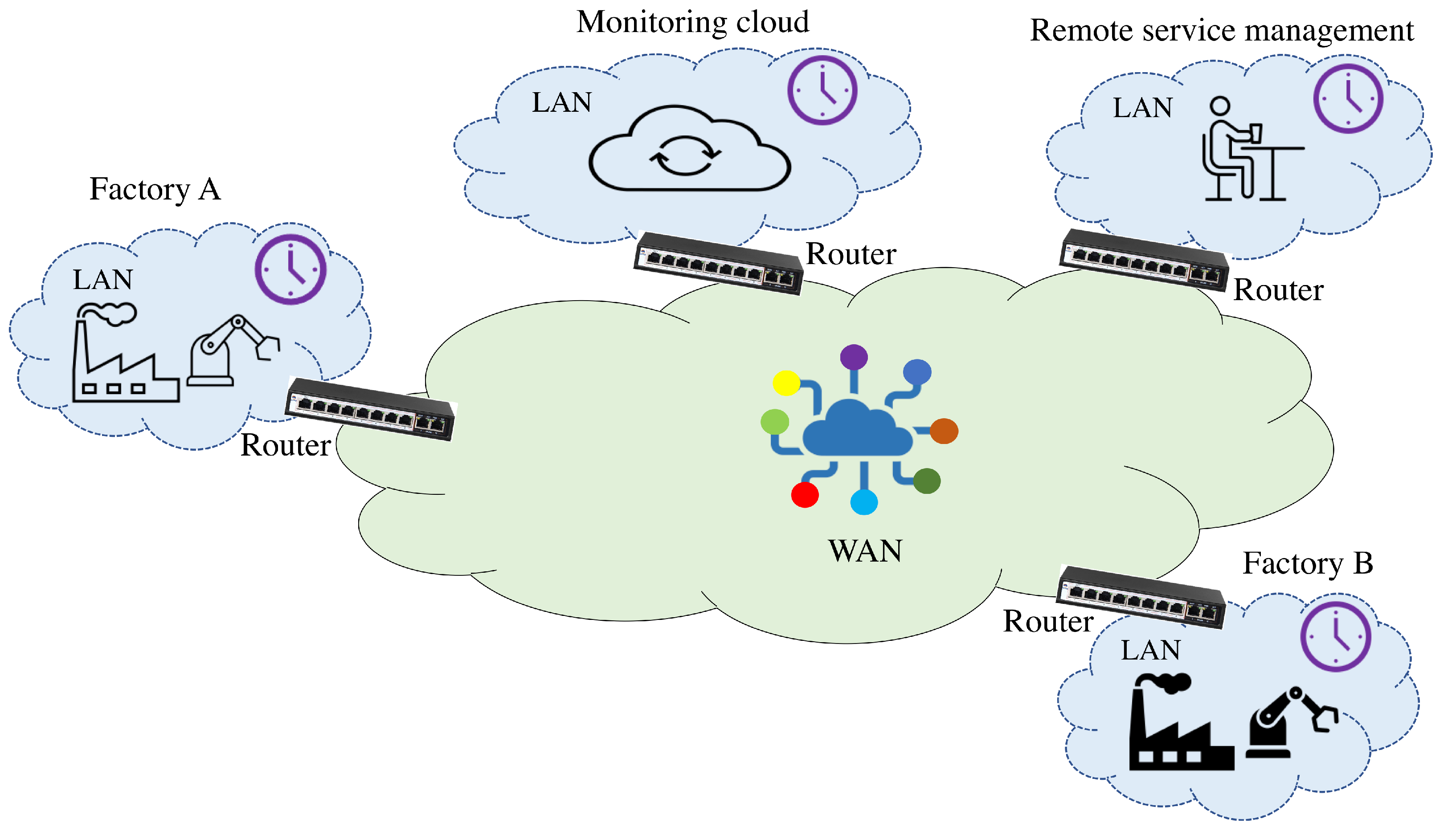
All such remote applications require factories to be connected to a remote site or another factory over a wide area network (WAN), as shown in Figure 1. A WAN is a geographically distributed heterogeneous communication network that interconnects wired and wireless segments from public and private networks, in which several communication technologies such as fiber optic link, Wi–Fi, Bluetooth, and Power Line Communication (PLC) are adopted.
Remote monitoring and control applications need a common notion of time for data consistency and coordination of activities among the factory and remote sites. A common notion of time is achieved by a clock or time synchronization service that aligns the clocks of all the devices on the network by distributing a common time to all nodes. The level of time accuracy and precision varies by application requirements, whereas remote maintenance of factory assets typically requires a second–level accuracy, while remotely controlling the factory valves will require a microsecond–level accuracy. Thus, the success of remote applications depends on the level of accuracy and precision of synchronization between a factory and remote site. Network packet delay variation or jitter adversely affects the clock synchronization accuracy. This effect is prominent in WAN as the different network segments contribute differently to end–to–end packet delays, e.g., the jitter of a fiber optics link is much less than the wireless links, resulting in variable end–to–end packet delays over time. The interference and noise levels over a WAN are significantly high. The unreliable communication networks result in higher events of missing packets and packet delay variation (PDV) than factory LANs such as wireless sensor networks (WSN). Thus, the heterogeneous nature and significant interference make it challenging to achieve an adequate synchronization over a WAN [3] compared to LANs.
Hardware–based and highly accurate clock synchronization solutions such as global positioning system (GPS) and precision time protocol (PTP) are prominent candidates for WAN. GPS is a satellite–based system that provides timing information to receivers on Earth; however, signal stability cannot be guaranteed for GPS. Having GPS at all distributed resources is also a costly solution. In addition, GPS is vulnerable to environmental conditions such as radio jams, resulting in signal loss and errors in synchronization. PTP is a network packet–based synchronization method that uses hardware time–stamps to compute delays. PTP requires hardware support to all the nodes to achieve a higher accuracy. Thus, it is not a cost–effective solution. Moreover, the management of PTP in a giant network such as WAN is challenging due to the complexity of the network structure, the difference of regional environments, the numerous and dispersed nodes, and limited fiber coverage. A software–based network time protocol (NTP) [4,5] is another network packet–based clock synchronization technique that uses software time–stamps to compute delays. NTP is easy to implement, deploy, and cost–effective compared to GPS and PTP. NTP is a promising clock synchronization solution for WAN, but it lacks in accuracy required for emerging remote monitoring and control applications.
In order to address these challenges, this paper proposes a software–based, scalable, yet accurate and precise clock synchronization algorithm for WAN called CoSiWiNeT based on Random sample consensus (RANSAC) algorithm to effectively deal with outliers in noisy offset data and predict correct clock offsets. For the evaluation of CoSiWiNeT, data measurements in a real WAN connecting two cities separated by 107 km were conducted. The results demonstrated that CoSiWiNeT outperforms NTP and state–of–the–art methods by achieving around 40% improved performance.
The contributions of this paper are as follows:
- (1)
- A scalable and precise clock synchronization algorithm based on RANSAC for heterogeneous WAN that provides improved synchronization over a degrading network condition has been proposed.
- (2)
- state–of–the–art methods typically use simulated network data or data from controlled environments, e.g., laboratories. The proposed algorithm is evaluated by means of simulation based on the data from real WAN with different degrees of network qualities—from good to degrading networks.
- (3)
- The algorithms’ performance was benchmarked against widely used in–practice time synchronization protocols such as NTP as well as state–of–the–art methods based on Kalman filter (KF) [6,7] and windowed least square (LS) [8] available in the literature. The proposed algorithm’s greatly improved performance with methods from practice and literature strengthens the new algorithm’s positioning.
The paper is organized as follows. First, related work is presented in Section 2. Section 3 describes the measurements from WAN and characterizes them. Section 4 introduces the CoSiWiNeT algorithm, and Section 5 evaluates its performance based on the measured network data. The conclusions have been provided at the end.
2. Related Work
Performance of software–based clock synchronization in terms of accuracy and precision fails to match their hardware–based counterparts due to device–level inaccuracies and unpredictable network conditions. Many methods have been described in the literature focusing on the performance improvement of software–based clock synchronization.
A large section of literature lists clock synchronization methods for wireless sensor networks divided into centralized and distributed synchronization. The centralized category uses the receiver–to–receiver principle, where one reference sender broadcasts packets and synchronizes a group of receivers with each other. They include Reference Broadcast Synchronization (RBS) described by J. Elson et al. [9] and S. Ganeriwal et al. [10] and Flooding Time Synchronization Protocol (FTSP) outlined by PulseSync [11] and several other works [12,13]. In contrast to centralized approaches, distributed time synchronization protocols rely on consensus algorithms to coordinate independent clocks in the network. They include Gradient Time Synchronization Protocol (GTSP) proposed by P. Sommer et al [14] and Average TimeSynch (ATS) described by L. Schenato et al [15]. F. Tirado-Andrés et al [16] present a methodology and a tool to choose an adequate time–synchronization strategy for wireless IoT end devices. L. Tavares Bruscato et al [17] proposed low–energy algorithms to converge the clocks of wireless sensor nodes quickly. More explicitly in the IoT domain, Sridhar et al. describe the CheepSync time synchronization protocol [18] for Bluetooth Low Energy (BLE) platforms. S. K. Mani et al. [19] developed a synchronization system, including a lightweight client, a new packet exchange protocol called SPoT. In another work, R. Gore et al. [20] proposed a lightweight clock synchronization algorithm called CoSiNeT for IIoT field devices. Recently, low–power Bluetooth or Wi–Fi beacons [21] have been proposed for synchronizing all the nodes of the network. All the above–listed methods are suitable for LANs where the field devices, e.g., temperature and pressure sensors, actuators, and low–end controllers, are resource–constrained and require a lightweight clock synchronization method in terms of memory and computation power.
In the case of WAN, remote systems that need to be synchronized are typically not resource–constrained in terms of computation power and memory. The higher noise and interference levels in WAN result in higher PDV compared to field IoT LANs. To deal with higher PDV, a computationally heavy clock synchronization algorithm can be realized for WAN. Several methods [22,23,24,25,26] have been proposed that extensively use the Kalman filter–based clock filter algorithm to estimate the server clock state (phase and frequency) from time offset measurements. The Kalman filter is ideal for random Gaussian errors in offset; however, it is sensitive towards packet delay outliers and occasional large spikes in offset. P. Jia et al. [27] proposed a digital–twin–enabled model–based scheme to achieve clock synchronization in IIoT environments. The success of this scheme depends on accurate clock modeling so that its behavior under dynamic operating environments is predictable. A batch least square (LS) based estimator to minimize the clock skew has been described by many works [28,29,30]. However, in LS, when the skew changes as a result of the ignored frequency drift term, its time offset estimates quickly deviate from the true values.
3. WANs: Time Data Measurement and Analysis
Delay and offset measurements in a WAN connecting two cities apart by 67 miles physical distance and 15 hops in network distance were conducted. The heterogeneous communication network includes mainly fiber–optics–based networks and various wireless networks such as Wi–Fi towards the endpoints. Four different network traces that represented different network conditions ranging from good to fair were selected. In this paper, the detailed measurement and analysis of the first two traces depicting deteriorating network conditions have been showcased, skipping traces from good network conditions. However, the results for all four traces have been summarized.
3.1. Network Data Capture Method
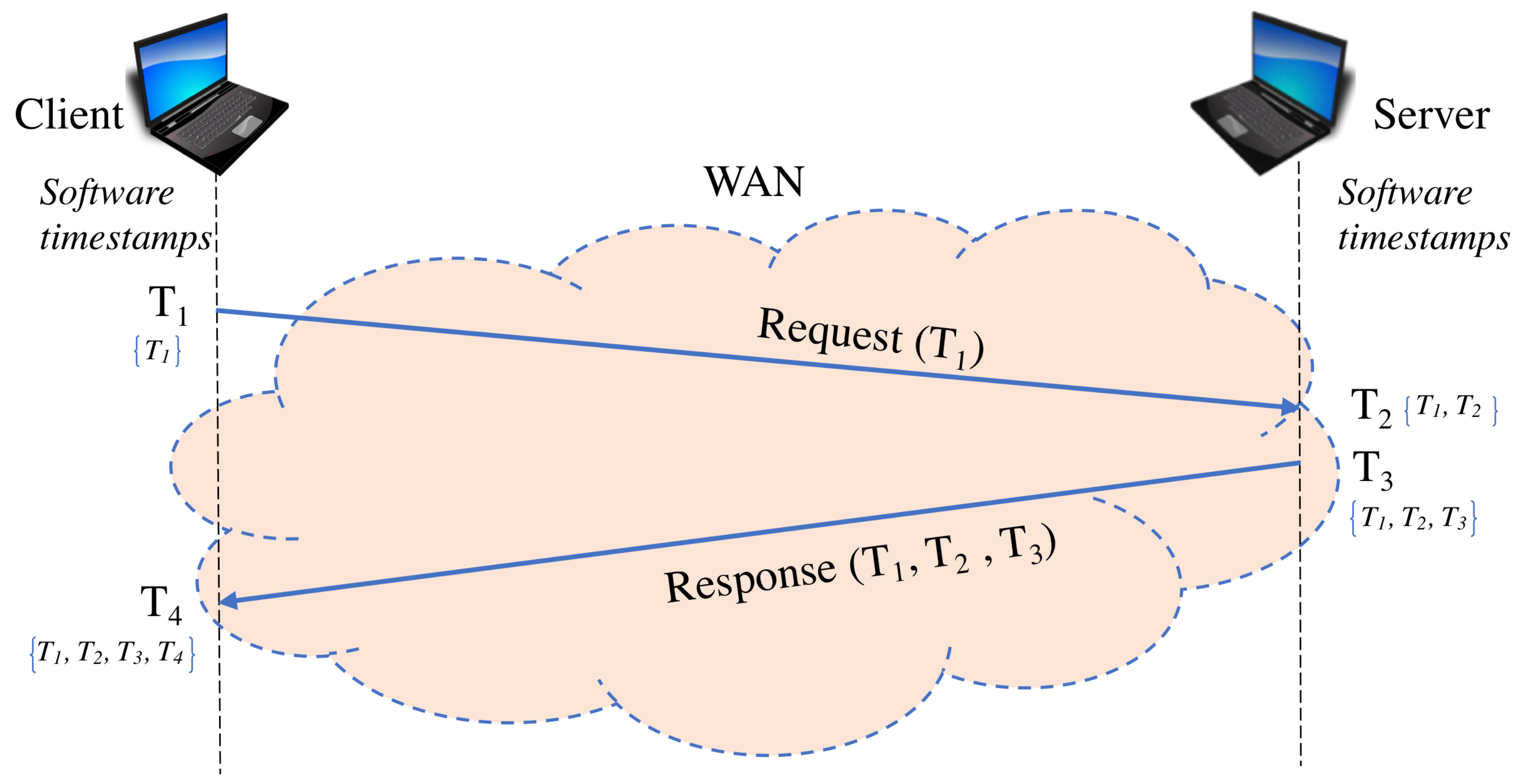
A client/server–based software application and two computers as depicted in Figure 2 to capture time–related network data were used.
The software tool running on the static host or client computer sends periodic timing requests containing the start time , to the static server computer via a communication network. The server acknowledges the request at the local time . The server then sends a reply at the time using the same timing packet with timestamps and . The host receives the timing packet back at time . Thus, the host machine accumulates , , , and timestamps corresponding to all periodic timing requests and responses over the same network for a particular period in a log file. The timestamps were used to calculate uncorrected time offset and round trip delays (RTD) between host and server machines using the formulas below.
This study did not consider the effect of coding languages and operating systems in software tool implementation on measurements as these factors are estimated to introduce a negligible difference in measurements.
3.2. Trace 1: Wide Area Network
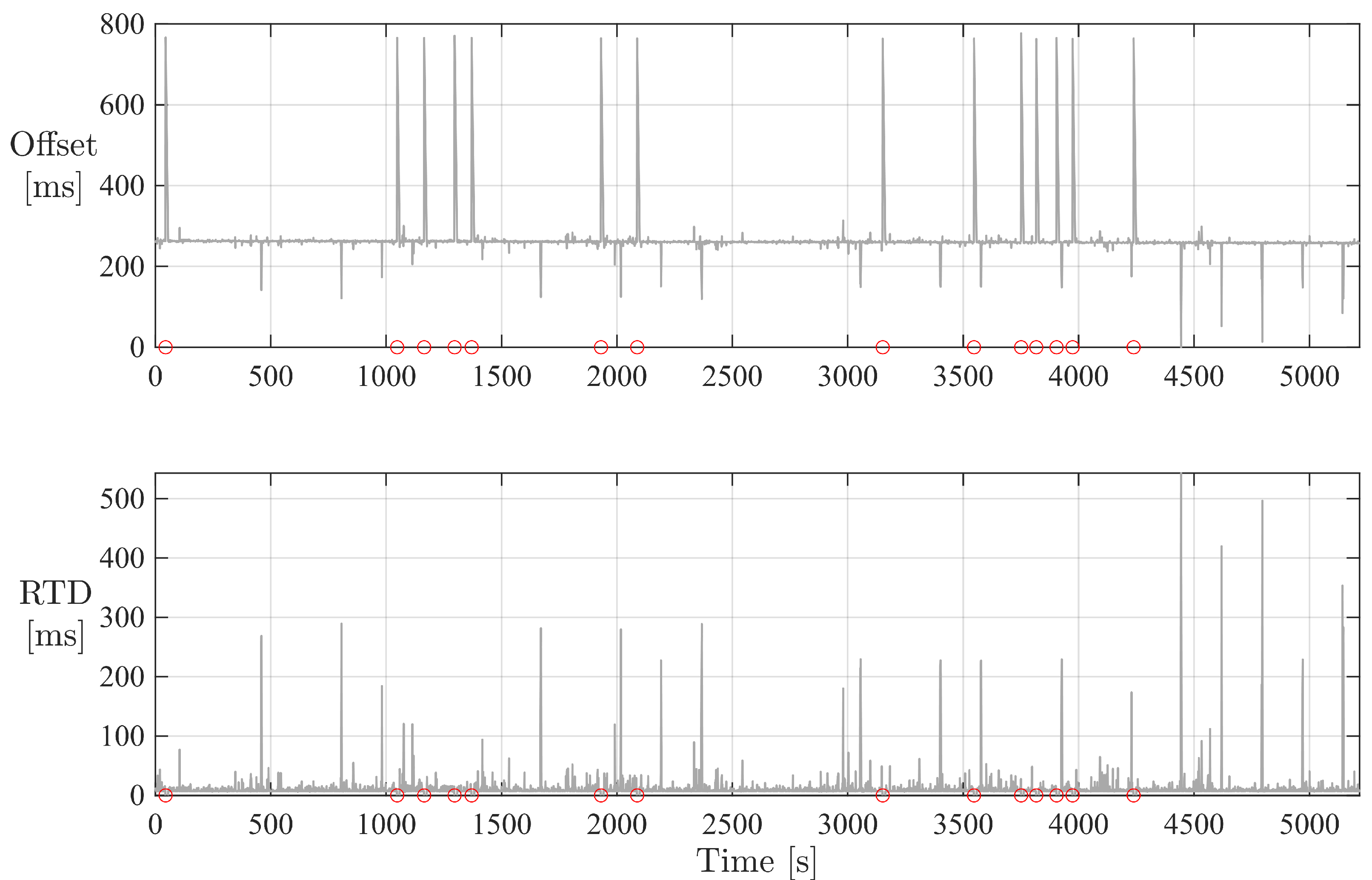
A WAN was analyzed by exchanging timestamps at a periodic interval of 1 s between client and server machines placed in two different cities. The corresponding raw, uncorrected offset and RTD values between a client and server are shown in Figure 3. The offset values have a mean of 261.1542 ms and a standard deviation of 29.0630 ms. The variation is due to occasional peaks up to 776.9609 ms corresponding to errors (marked in red circles) due to incomplete or missing timing requests and responses. RTD values over time are distributed with a mean of 10.9815 ms and a standard deviation of 22.7386 ms. The peak–to–peak RTD value is 540 ms owing to higher peaks of the order of 545 ms towards the end in line with downward peaks in offset values.
3.3. Trace 2: Wide Area Network
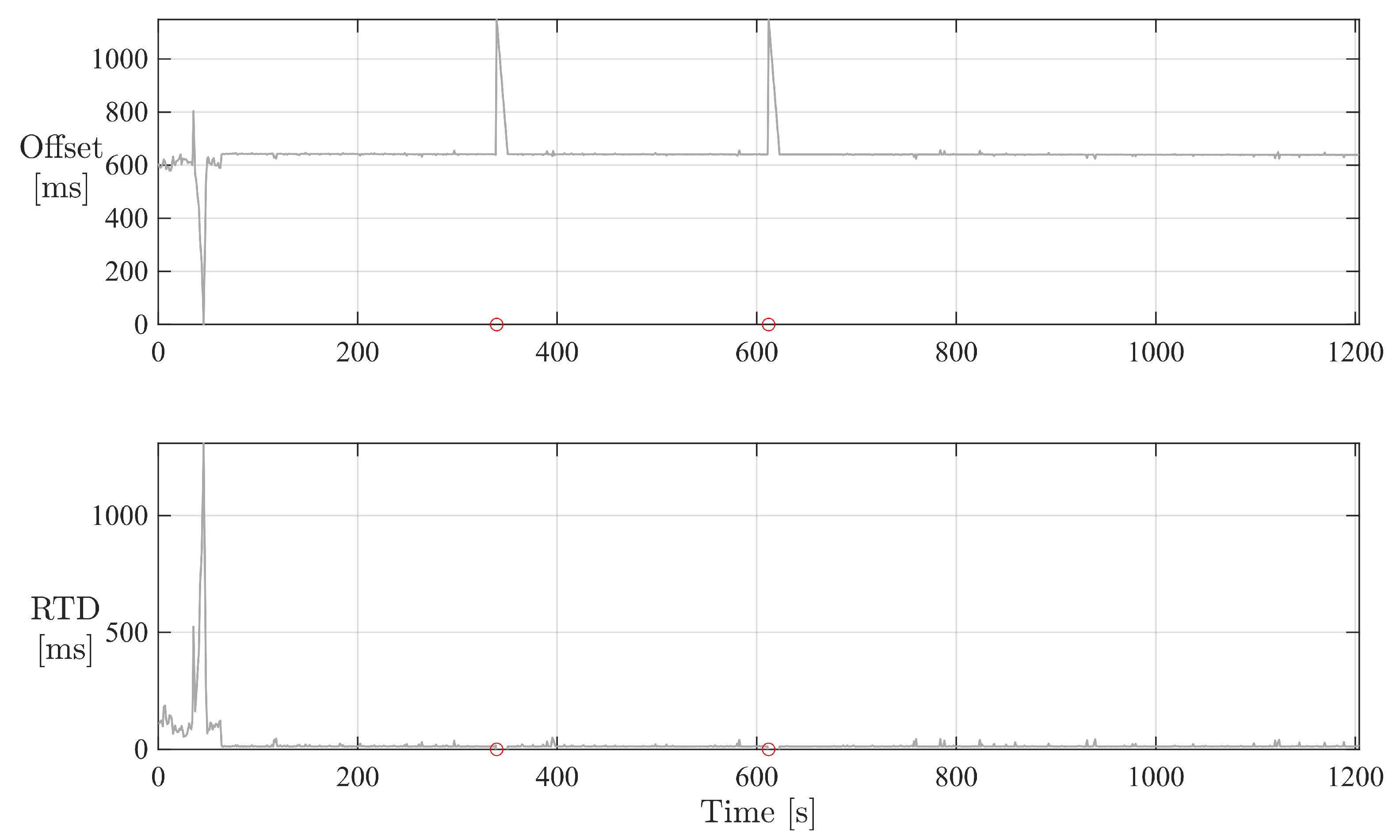
The same WAN was analyzed at different times by exchanging periodic timing messages between the same client and server machines in two cities. The resulting raw, uncorrected offset and RTD value over time are shown in Figure 4. The offset values are distributed with a mean of 638.5867 ms and 34.3873 ms standard deviation. The higher variation in offset is due to two outliers in the order of 1147 ms when two errors (marked in red circle) were observed during timing message exchange, and an undershoot in the beginning. The occasional peaks and an undershoot resulted in a higher peak–to–peak offset of 1147.9437 ms in otherwise stable offset values. RTD values are distributed with a mean of 20.5277 ms and 57.6120 ms standard deviation. The higher variation in RTD is due to one overshoot in the order of 1308 ms when there was an abrupt change in offset in the beginning, represented by an undershoot. This single peak resulted in a higher peak–to–peak RTD of 1298 ms in otherwise stable RTD values.
3.4. NTP Measurement in Wide Area Network
The same WAN was also analyzed by exchanging NTP messages at a variable polling interval decided by the NTP algorithm between two machines placed in two different cities. The server machine was configured as a ‘NTP server’ and the client machine as a ‘NTP client’. The NTP server itself was synchronized to the nearby stratum–2 public server from the NTP pool infrastructure. The ‘NTP client’ synchronizes to the ‘NTP server’ by continuously exchanged NTP messages carrying timestamps. The time and frequency offsets resulting from the NTP algorithm were stored in various log files such as loopstats and peerstats. These values were used for comparing NTP performance with other clock synchronization methods.
3.5. Summary: Network Time Data Measurement
All the measured network traces by their network types, and communication medium have been summarized in Table 1.
The lowest timing request error rate (TRER) are 0 for ‘Trace 4’ and 0.00075 for ‘Trace 3’ of WAN measurements. ‘Trace 1’ and ‘Trace 2’ have comparatively higher TRER. Typically, heterogeneous WANs comprising of multiple segments of wired and wireless networks from public and private domains are non–deterministic and susceptible to various noise sources, often missing and delaying packets. Thus, a finite TRER includes one or more failures in exchanging timing requests and responses and indicates a possible deterioration of the network. A criteria to define network conditions (good, fair, or poor) based on that network’s TRER value were developed. Using this criterion, traces 1 and 2 were defined as from a ‘Fair’ network, trace 3 from a ‘Fair (Low)’ network, and trace 4 from a ‘Good’ network.
4. CoSiWiNeT: RANSAC–Based Clock Synchronization Algorithm
Unpredictable communication network performance often leads to delayed, incomplete, or missing data packet transfers, resulting in a noisy clock offset and delay measurements. Curve or line fitting algorithms for clock synchronization are being explored for their ability to deal with the effects of network bursts and surges. However, curve fitting becomes challenging in the presence of noisy data, outliers, and missing data. Furthermore, data may not always fit the model precisely because of measurement or detection noise and intra–class variability. A clock synchronization algorithm called the CoSiWiNeT based on RANSAC was proposed, which performs better than LS methods in the presence of outliers or noisy offset data.
CoSiWiNeT converts an estimation problem in the continuous domain into a selection problem in the discrete domain. For example, if there are 100 data points to fit a line, LS would use 2 points, whereas there are or 4950 possible ways to fit a line. CoSiWiNeT chooses the best suitable pair among 4950 options. To do so, the CoSiWiNeT algorithm iteratively executes two steps: hypothesis formation and evaluation of framework, as shown in Algorithm 1.
| Algorithm 1 CoSiWiNeT algorithm |
| Inputs: Measured offset, Function f computes model parameters p given a sample S from U, Minimum number of offset samples required to estimate model parameters, n Maximum number of iterations, k Error tolerance threshold, t Minimum valid consensus threshold, d Outputs: Model parameters fit best to offset data,
|
In the first step, a minimal sample set of size n is randomly selected from the input dataset of size N. Then, the model parameters are computed based on an earlier selected random sample set. The elements of a random set (n) are smallest sufficient to determine the model parameters in contrast with other methods such as LS, where the model parameters are estimated using all the data points (N) with appropriate weights. In the evaluation step, the error function is calculated for each data point. CoSiWiNeT checks which elements of the entire dataset are consistent with the selected model whose parameters have been estimated in the first step. The data elements which do not fit the model within some error threshold attributed to the effect of noise are called outliers (O). Thus, CoSiWiNeT selects the remaining data elements that support the current hypothesis. The set of such elements is called consensus set () or inlier set (I) [31,32].
CoSiWiNeT executes iteratively for k times and terminates when the probability of finding a better–ranked drops below a certain threshold. The total number of inliers typically decides the ranking. A that contains more elements is ranked better than a that contains fewer elements. The total number of iterations that are required to ensure, with a probability p, that at least one random sample produces an inlier set that is free from “real” outliers is given by
It can be learned that k can be very large if p gets closer to one. For a fixed p, k can be made smaller if is made larger or n is made smaller.
The CoSiWiNeT algorithm is implemented with a moving window–based approach. The algorithm predicts a new offset value based on the best fit linear curve to the previous window of data elements. In the current design of the 200 element window, the algorithm starts working by predicting the 201st offset based on first 200 offset values. The algorithm then predicts 202nd offset value based on moved window of elements 2 to 201.
CoSiWiNeT is an easily implementable method to fit the curve to noisy data with many outliers. On the downside, there are many parameters to tune for a better fit; it may need many iterations to get the expected accuracy and requires the inlier to outlier ratio to be reasonable.
5. CoSiWiNeT Evaluation
The CoSiWiNeT algorithm’s performance was evaluated using the four network traces with different conditions, summarized in Table 1. Various parameters such as predicted time and frequency offsets, offset error, and execution time were used for the algorithm evaluation. The proposed algorithm’s performance was also compared with NTP and state–of–the–art methods based on KF and LS to derive the baselines. To make the proper comparison, raw or uncorrected offsets from free–running clocks in server and client devices were captured as described in Section 3. The uncorrected offset values captured over a long time were fed as an input to all the algorithms implemented in a Matlab simulator. The behavior of each algorithm captured in terms of how effectively they correct the offset was visualized and analyzed in Matlab.
5.1. Predicted Clock Offset
The accuracy and precision of a clock synchronization algorithm depend upon the variability in clock offset and RTD values. Thus, the algorithm which reduces the variability in raw offset measurements the most can be assured to provide a better clock synchronization performance.
5.1.1. Network Trace 1
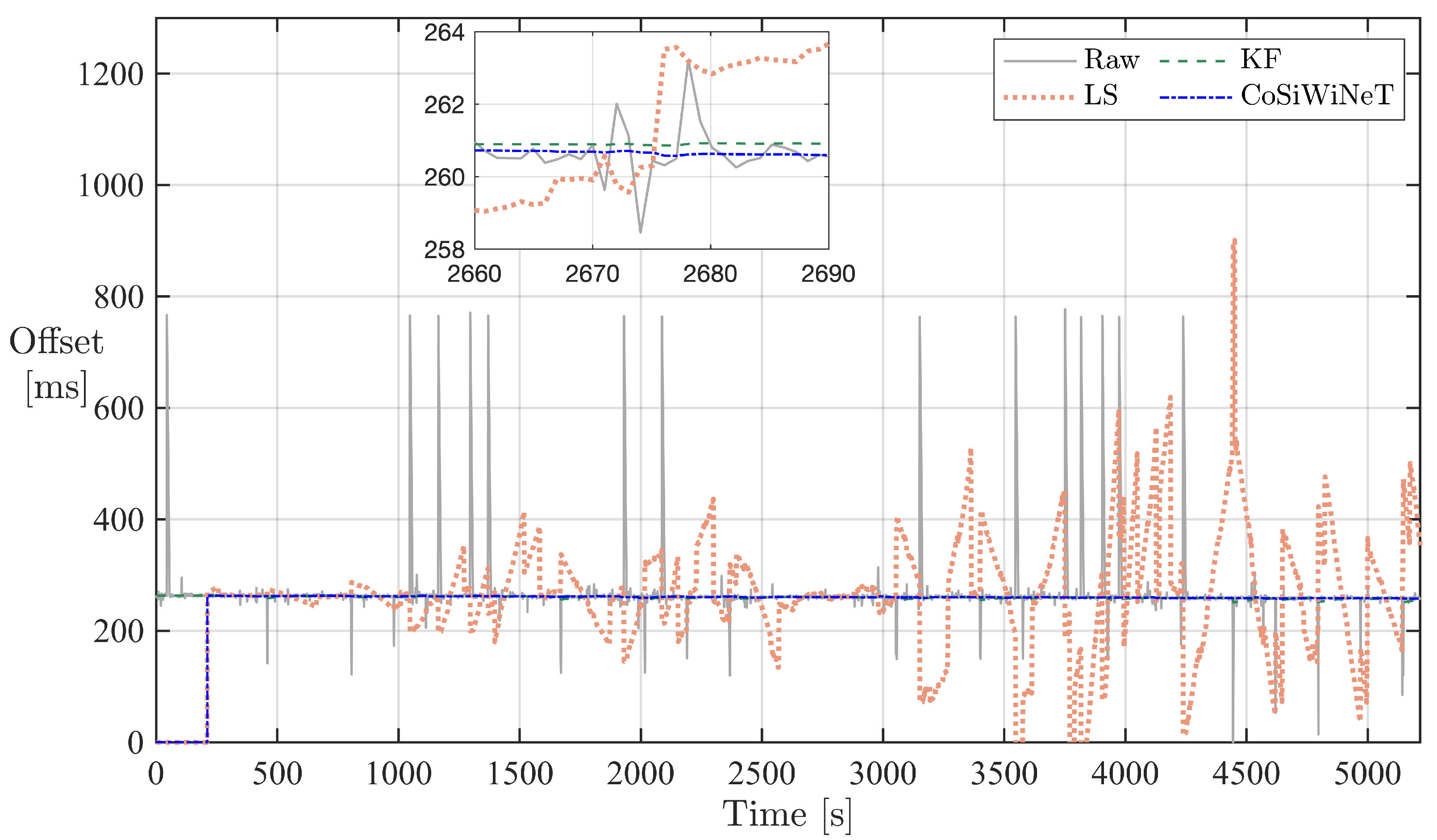
The clock offset output of algorithms, KF, LS, CoSiWiNeT, along with the raw input clock offset for trace 1 are shown in Figure 5. The outliers in raw clock offset represented by spikes are minimized by all these algorithms, more evidently by KF and CoSiWiNeT. However, LS shows additional spikes in its clock offset output.
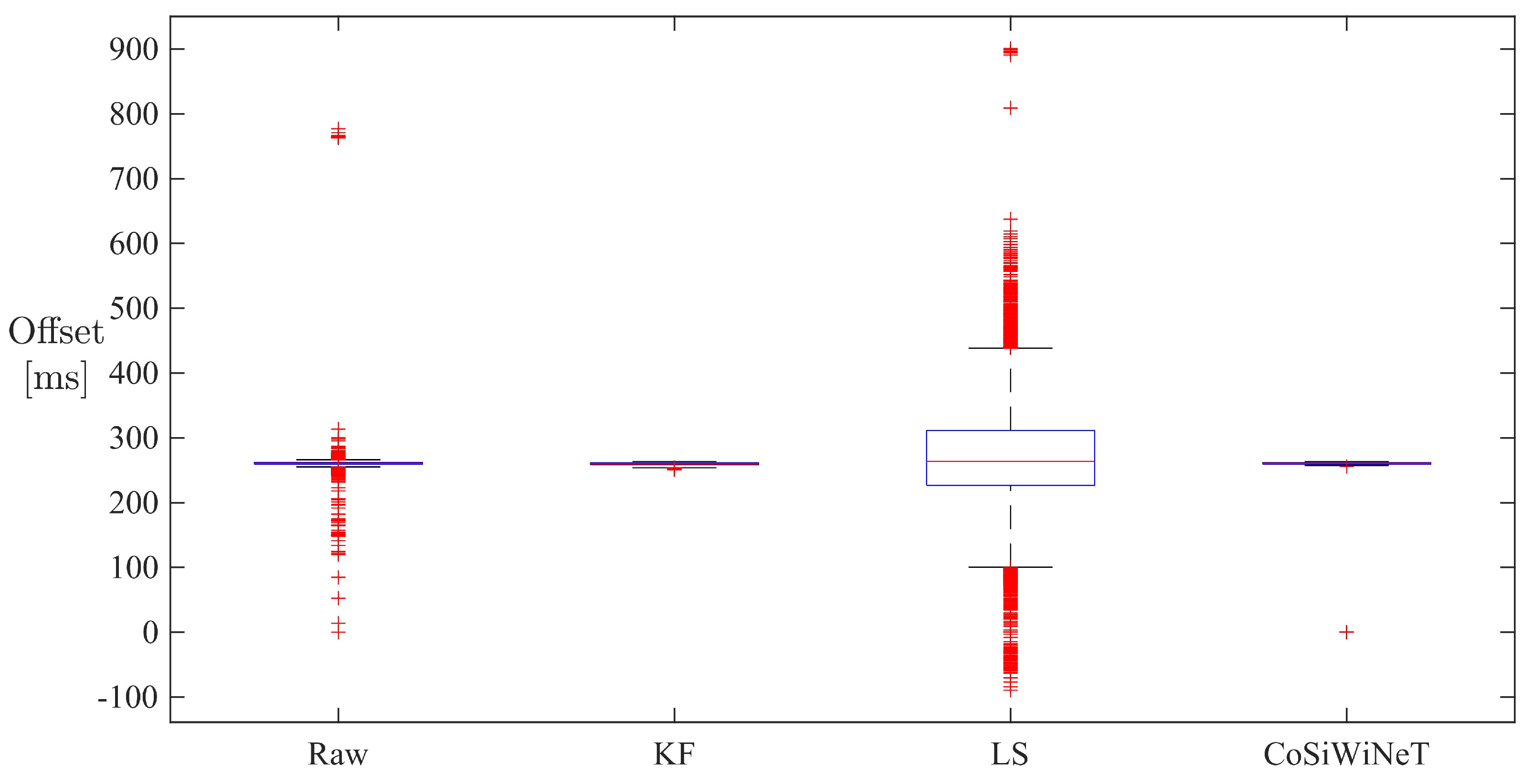
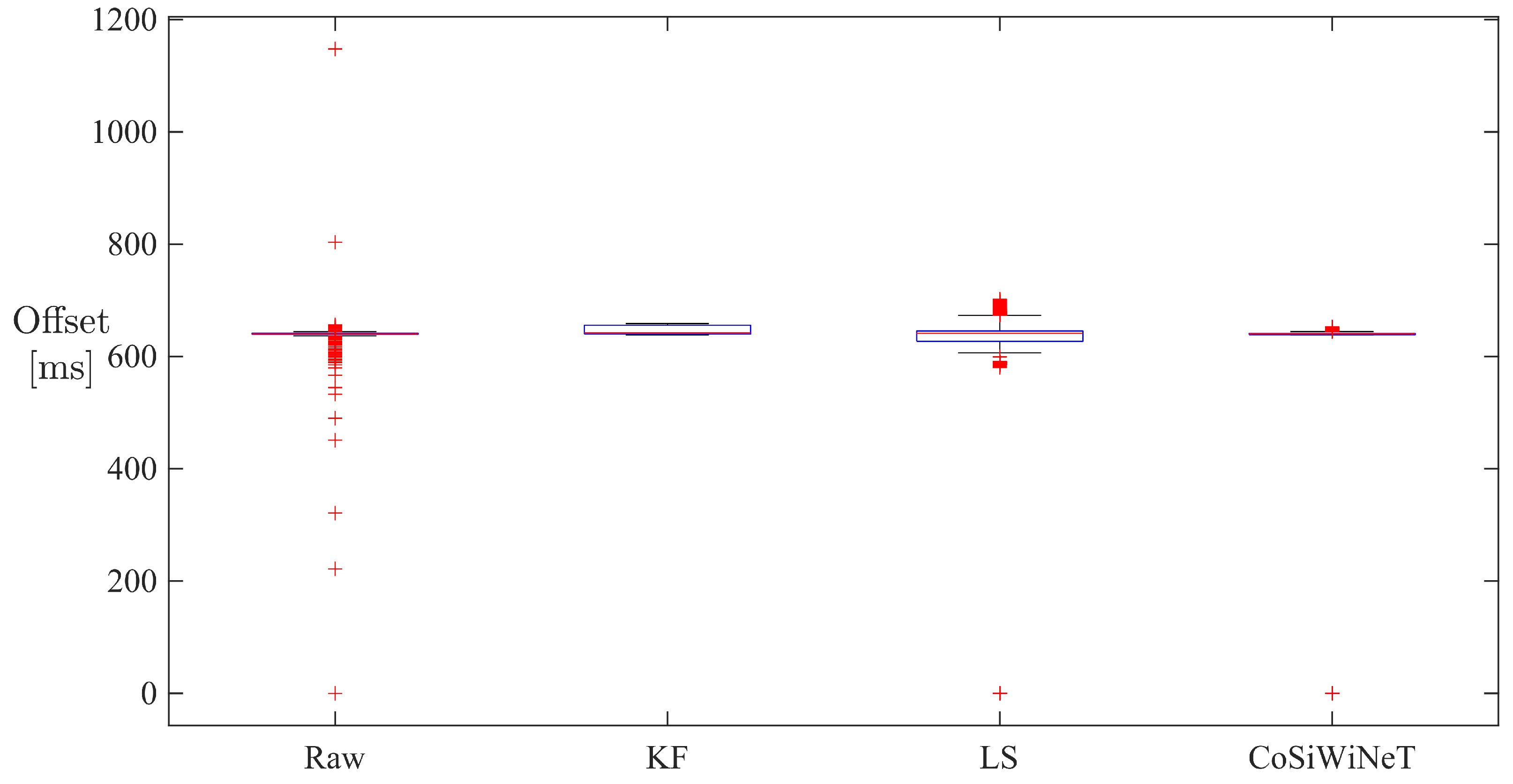
To formulate the variability of responses, a box–plot representation of input and output offset values for various algorithms is shown in Figure 6.
The interquartile range (IQR), the measure of variability, is represented by a height of the box, and it indicates the spread of data in a data set. The IQR of KF, LS, and CoSiWiNeT is 1.4804, 37.8196, and 1.077, respectively, compared to 1.3908 of a raw offset, which indicates that CoSiWiNeT performs better than KF and LS.
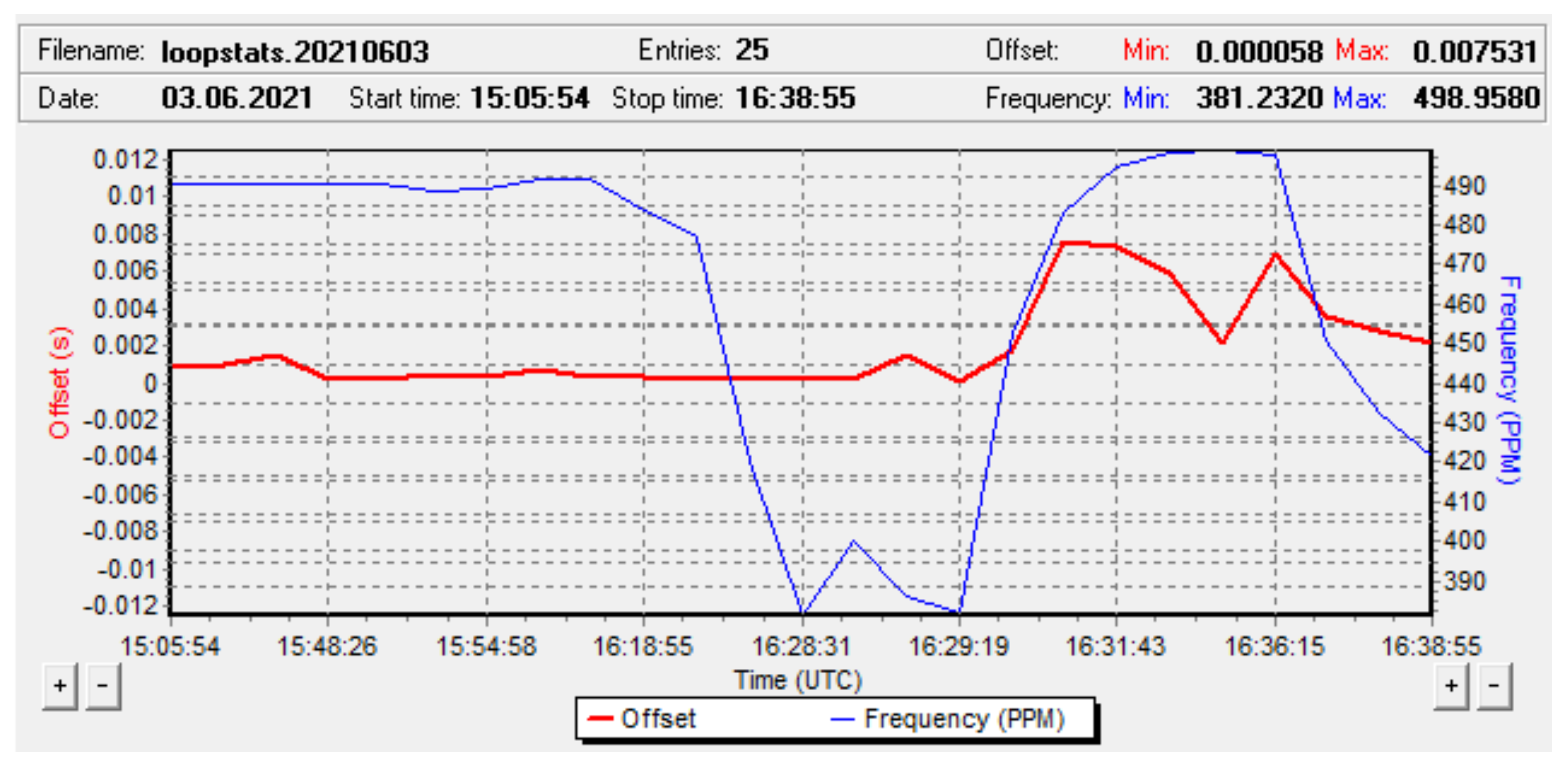
The output of the NTP algorithm, i.e., the corrected offset is shown in Figure 7.
The corrected offset values ranges from 0.058 ms to 7.531 ms. The clock frequency varies from 381.23 ppm to 498.95 ppm.
5.1.2. Network Trace 2
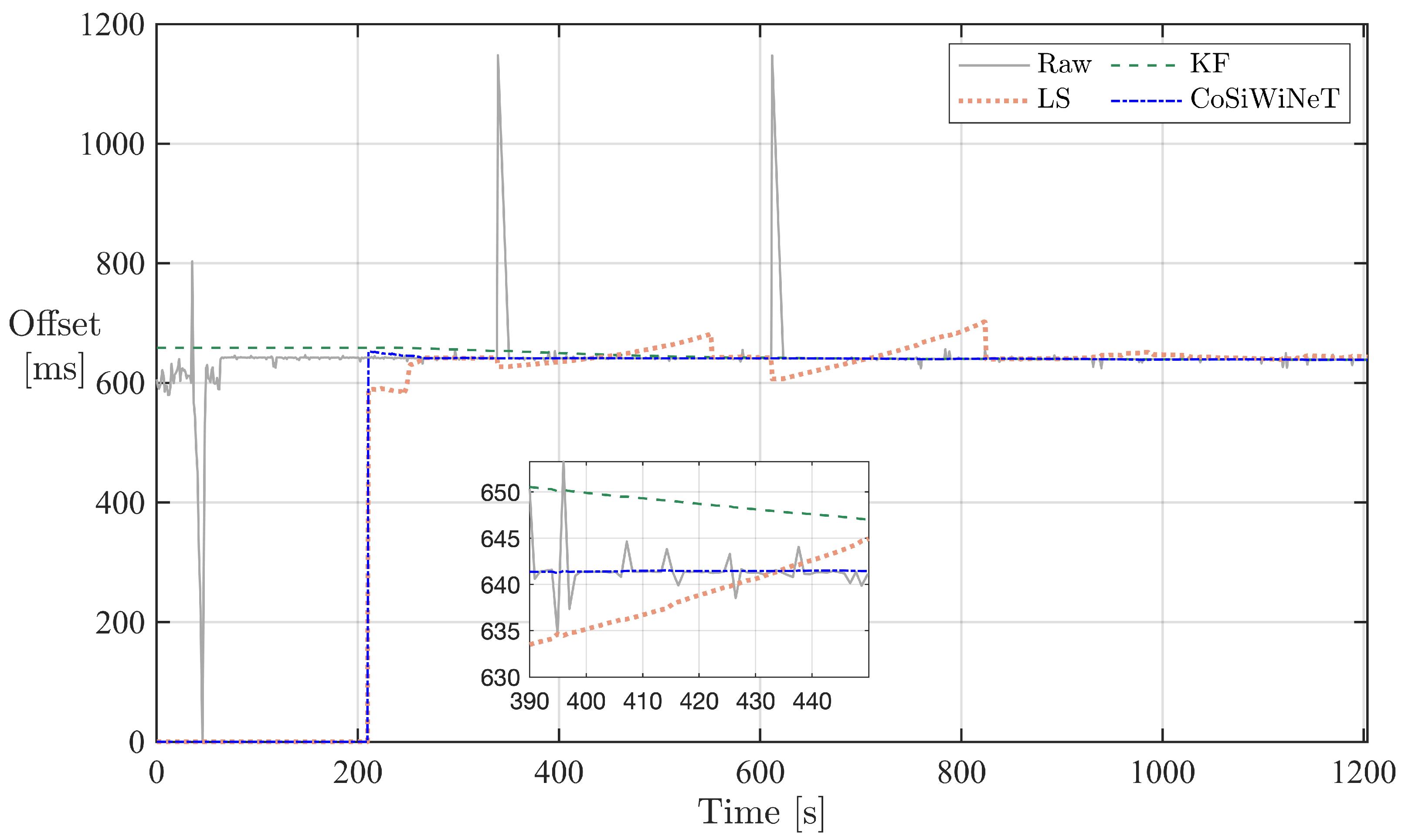
The comparison of raw clock offset from trace 2 and clock offsets filtered by synchronization algorithms is shown in Figure 8. The moving window–based LS and CoSiWiNeT algorithms start working from 201st offset data and reduce the two visible peaks of raw clock offset. However, the LS does introduce few new peaks while correcting the input offset.
The graphical view of depicting the comparison of predicted clock offsets with the raw one is represented by box plots as shown in Figure 9. The IQR values 0.9332, 3.5078, 3.4392, and 0.9892 of raw input, KF, LS, and CoSiWiNeT, respectively, show that CoSiWiNeT does perform better than KF and LS.
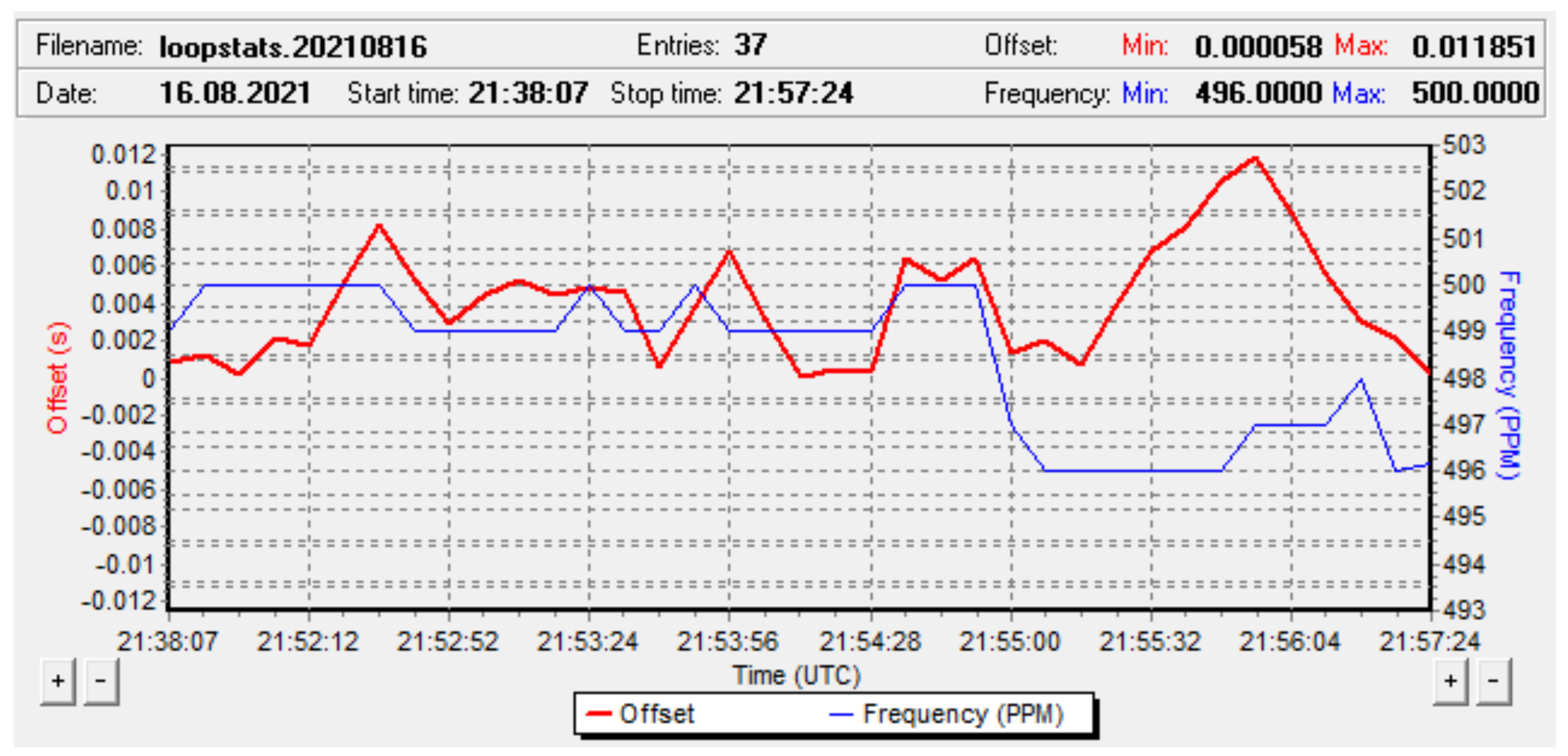
The corrected offset output of the NTP algorithm is shown in Figure 10. The corrected offset values ranges from 0.058 ms to 11.851 ms. The clock frequency varies from 496 ppm to 500 ppm.
5.1.3. All Network Traces
The NTP offset measurements were conducted simultaneously with raw offset measurements in the same WAN. To compare the outcomes of such related measurements based on the variability of predicted offsets, a statistical parameter called ‘coefficient of variation (CV)’ [33] was used. CV is a statistical measure of the relative dispersion of data points in a data series around the mean. It is calculated as the ratio of the standard deviation to the mean (average). As shown in Table 2, the CV is lowest for CoSiWiNeT in the case of trace 1 (41.86% and 39.13% improvement over NTP and KF, respectively) and trace 2 (35.39% and 40.33% improvement over NTP and KF, respectively). In the case of trace 3, the CV of CoSiNeT is lower than raw input and LS but comparable with KF and NTP. In trace 4, the CV of all the algorithms is almost comparable.
5.2. Predicted Frequency Offset
The frequency offset is closely related to clock offset (time). It can be calculated as
The algorithm that reduces the most variability in raw frequency offset values assures the best clock synchronization performance.
5.2.1. Network Trace 1
The raw frequency offset and filtered frequency offsets by KF, LS, and CoSiWiNeT for trace 1 are shown in Figure 11. The higher variability in raw frequency offset can be seen through multiple spikes though out the duration of trace 1. The visual inspection confirms that all the algorithms manage to curb the raw frequency offset variations.
To quantify the individual performance of algorithms, a box–plot representation of raw input and outputs of algorithms is shown in Figure 12. The IQR of KF, LS, and CoSiWiNeT 3.2449, 16.7254, and 2.3331 compared to 478.2144 of a raw frequency offset indicates that CoSiWiNeT performs better than KF and LS.
5.2.2. Network Trace 2
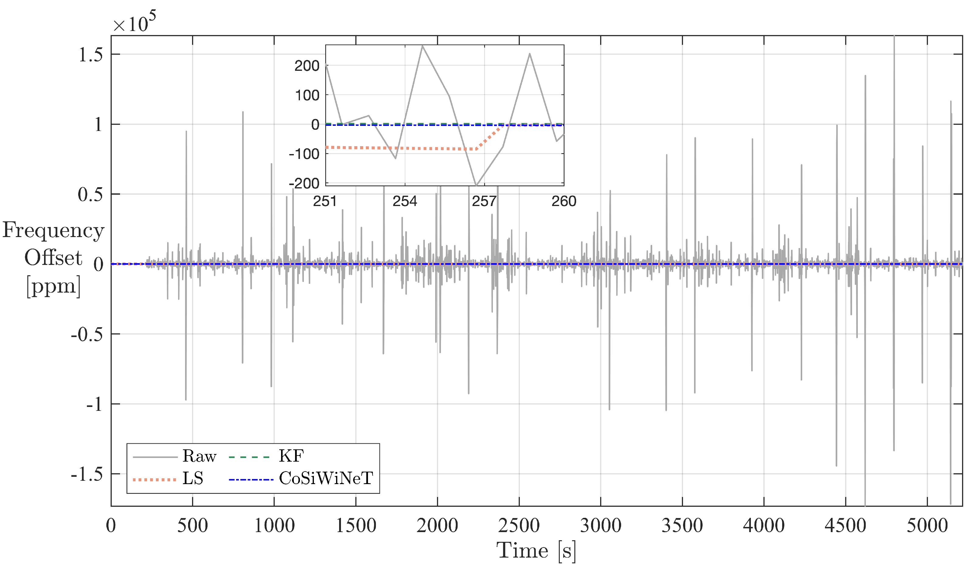
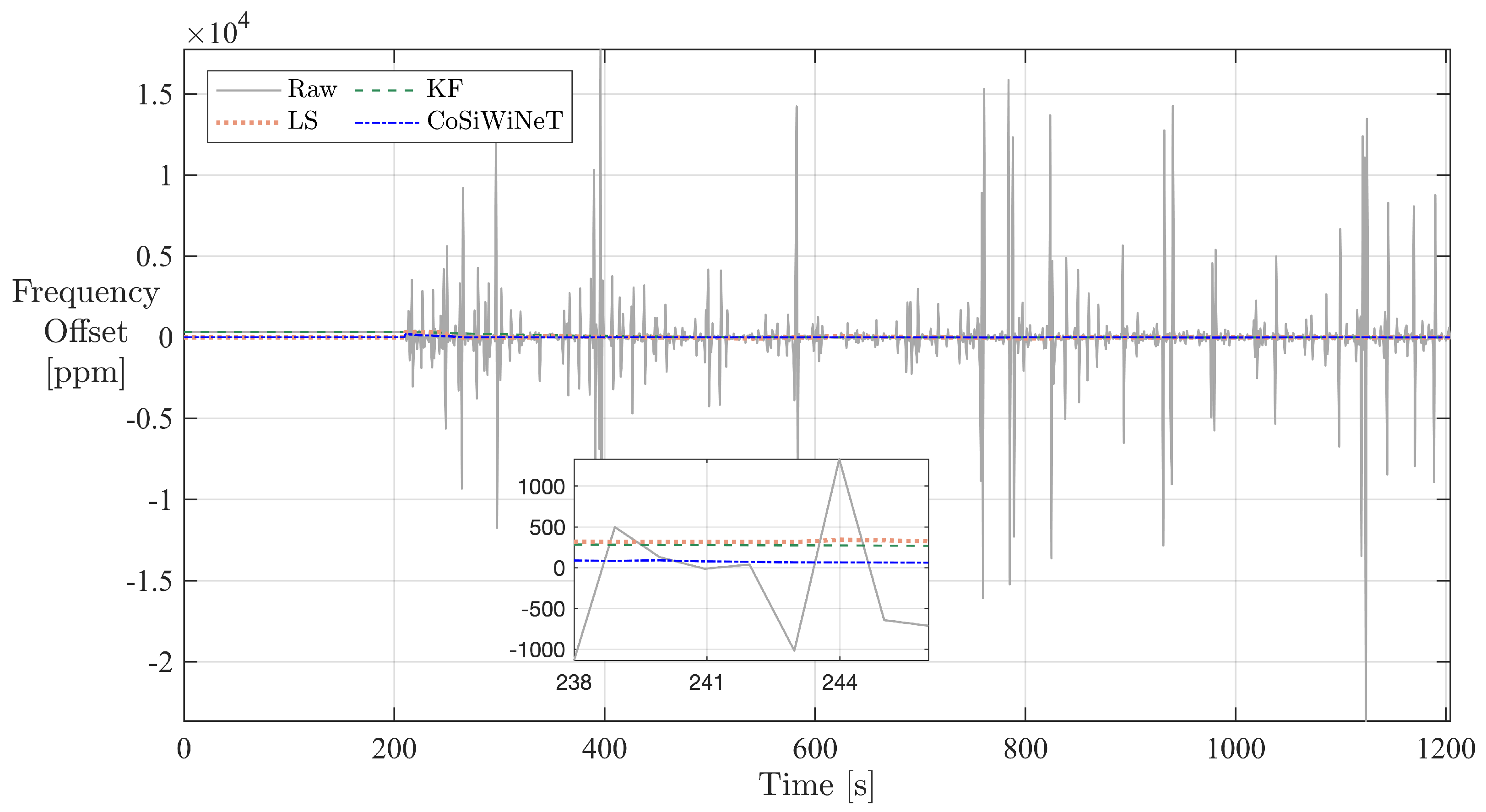
The raw frequency offset and filtered frequency offsets by KF, LS, and CoSiWiNeT for trace 2 are shown in Figure 13. The outliers represented by higher magnitude spikes in raw frequency offset values indicate higher variability. This variability is reduced by all the algorithms to large extent.
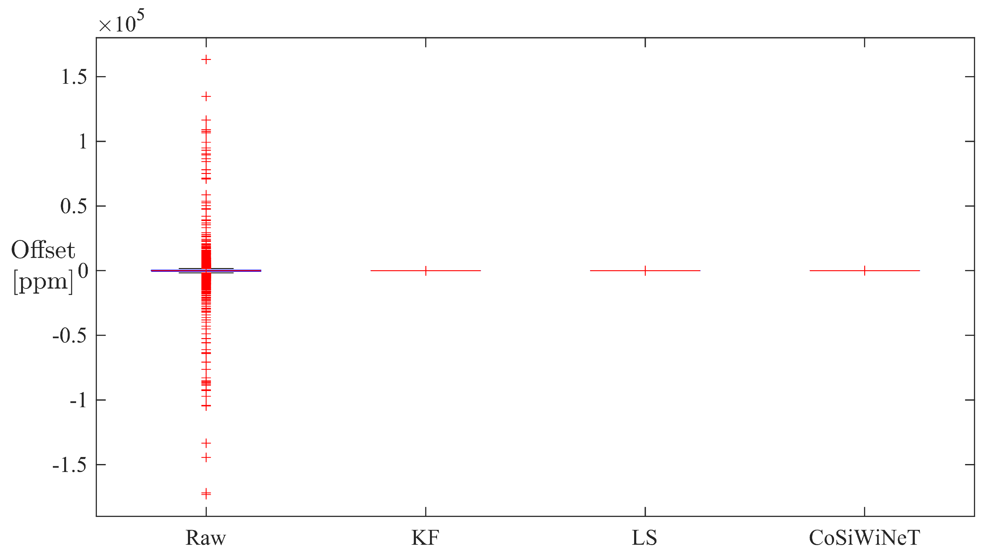
A box–plot representation comparing raw input frequency offset with filtered frequency offsets is shown in Figure 14. The IQR of KF, LS, and CoSiWiNeT is 92.1462, 3.0341, and 1.5511, respectively, compared to 214.8646 of a raw frequency offset, indicating that CoSiWiNeT performs better than KF and LS.
5.3. Clock Offset Error
The clock offset error was calculated as a difference between filtered or corrected clock offset and ideal clock offset values for each measurement sample. As the raw and uncorrected input offset values are increasing or decreasing over time, the ideal clock offset profile was considered to follow a straight line passing through raw offset values. Therefore, the clock offset error should be zero for the ideal clock synchronization algorithm. In practice, the synchronization algorithm with minimum offset error is considered to be the best algorithm.
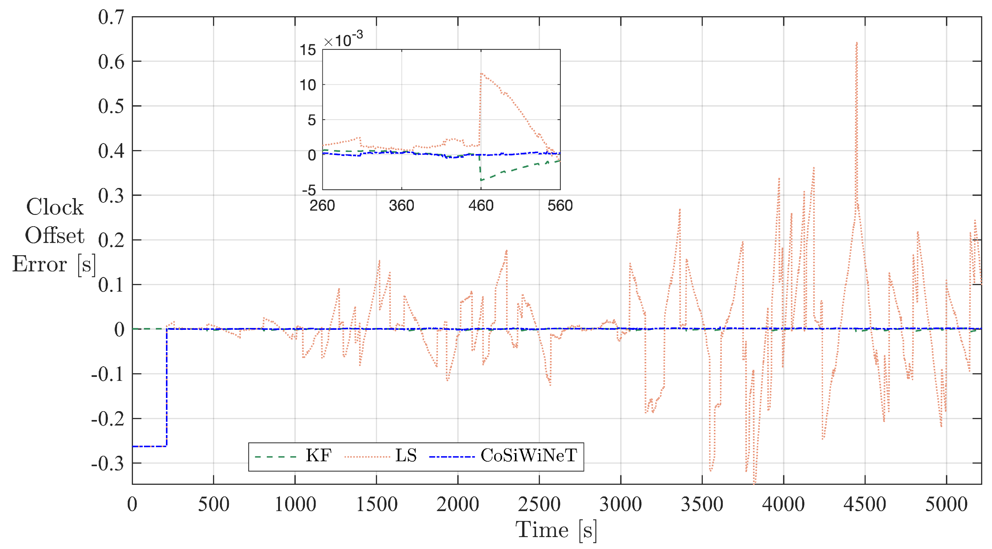
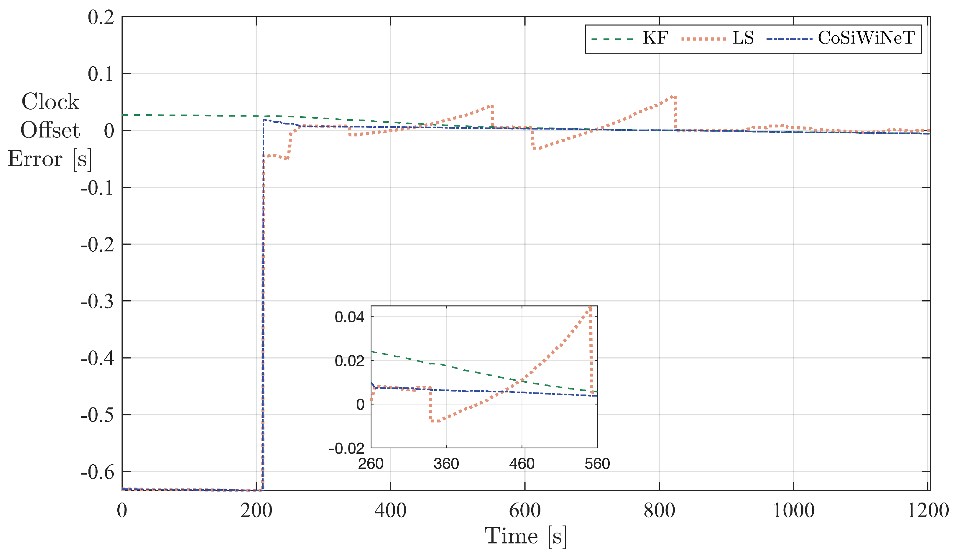
The clock offset error profiles of KF, LS, and CoSiWiNeT for network traces 1 and 2 are shown in Figure 15 and Figure 16, respectively. Both error profiles show that KF and CoSiWiNeT produce lower offset errors compared to LS. The magnified views on both figures reveal this fact more clearly.
To quantify the error performance of synchronization algorithms, a statistical parameter called root mean square error (RMSE) was used. RMSE is the standard deviation of the residuals (prediction errors), and it informs how concentrated the filtered offset data is around the line of the best fit. RMSE for raw input as well as output offset values of various synchronization algorithms is shown in Table 3. In network traces 1 and 2, the RMSE of CoSiWiNeT is lower than RMSE of raw and synchronization algorithms KF and LS. In the case of traces 3 and 4, the RMSE of CoSiWiNeT is lower than RMSE of raw and LS, but it is comparable with KF.
5.4. Algorithm Execution Time
The clock synchronization algorithms were also compared based on execution time. The execution time was considered as a full processing time of one new offset data sample through a clock synchronization filtering algorithm. The ‘tic’ time is stamped when a new sample is available for processing, and the ‘toc’ time is noted when a predicted offset is available. Various execution times calculated as a difference between the respective ‘tic’ and ‘toc’ timestamps are shown in Table 4. The average execution time of KF is lowest at 6.23 µs, with LS and NTP following closely at 32.02 µs and 61.53 µs. The average execution time of CoSiWiNeT algorithm is 18.4 ms. As CoSiWiNeT executes multiple iterations (e.g., 500 in this case) and selects the best for a single offset data prediction, its execution time is comparatively higher than others. The execution times were measured on laboratory computing machines, and the effect of different machine configurations, operating systems were not considered for this analysis.
5.5. Results and Validity
The clock synchronization algorithm’s essential function is to reduce the variability in raw offsets introduced by packet delay variation in a network. Therefore, a better–performing clock synchronization algorithm is the one that curbs this variability more effectively. For performance comparison of different clock synchronization methods, various parameters such as (i) predicted clock offset, (ii) predicted frequency offset, (iii) clock offset error, and (iv) algorithm execution time were used. The results of network trace 1 and 2 reveal that CoSiWiNeT performs better than state–of–the–art KF algorithm, LS algorithm, and state–of–the–practice NTP protocol on the first three parameters. The results of traces 3 and 4 reveal that the performance of CoSiWiNeT is almost comparable with state–of–the–art KF algorithm, LS algorithm, and state–of–the–practice NTP protocol on the first three parameters. However, the fourth parameter, execution time, indicates that CoSiWiNeT achieves better performance at the cost of a longer execution time (18.4 ms) compared to KF, LS, and NTP (maximum 61.53 µs).
The evaluation of of a new clock synchronization algorithm could be done in various ways. First, using test data obtained from live network characterization as a stimulus to the Matlab program and measuring the time metrics; second, using live data obtained from real industrial sites as a stimulus to Matlab program and measuring the time metrics and thirdly implementing the software solution on a hardware platform and using the same in real industrial networks and measuring the time metrics. All the above evaluation methods of a new clock synchronization algorithm vary in terms of their degree of confidence. However, practical difficulties such as availability of industrial network data or access to industrial sites for experimentation, can act as bottlenecks. The possible approach of comparing performance of various state–of–the–art algorithms with CoSiWiNeT is to run these algorithms simultaneously on different devices in the same network. However, in this case, network conditions and host device activities experienced by all algorithms would possibly not be the same at all time and thus the comparison may not be fair. To deal with the above–mentioned practical difficulties, the raw and uncorrected offset data obtained from a real WAN was used as a stimulus to validate the performance of CoSiWiNeT and compare it with KF and LS methods. Without theoretical analysis of the network, the generalization of results based on experimental evaluation can be limited. To increase the confidence in results, the longer network traces with different degrees of network conditions were used for evaluation. Such analysis of realistic case studies reduced the threats to the validity of results.
6. Conclusions
Clock synchronization for distributed sites using WAN is essential for realizing emerging automation applications based on remote monitoring and control of factory sites. GPS and PTP can be prominent hardware–based solutions to achieve accurate clock synchronization; however their use is challenged by cost, unavailability of continuous GPS signals due to environment, and hardware failure modes. As the existing software–based solution, NTP overcomes these challenges but lacks in accuracy, for WAN a scalable, software–based clock synchronization algorithm called CoSiWiNeT was proposed. The new algorithm’s performance was evaluated by means of simulation based on parameters, predicted clock offset, frequency offset, offset error, and execution time. Based on the first three parameters, the evaluation shows that the CoSiWiNeT algorithm matches well NTP and state–of–the–art method based on Kalman filter in a good network environment, but performs better by 41% and 40%, respectively, in fair and deteriorating network conditions. The downside of the CoSiWiNeT algorithm is comparatively higher execution time. However, for a polling rate of 1 s, this execution time is fast enough to predict offset before the next sample measurement. Furthermore, the algorithm can successfully deal with offset changes due to step changes in RTD and multiple errors in timing messages due to network deterioration, improving system reliability and safety.
Having evaluated the functional performance of CoSiWiNeT in terms of accuracy and precision, as a future step, the other aspects such as availability, scalability on different hardware platforms, and performance in distributed topology comprising multiple master or server devices can be studied further. In clock synchronization systems, the devices, as well as the synchronization related communication messages are prone to security incidents and thus security issues can be investigated for identifying effective measures.
Author Contributions
Conceptualization, R.N.G., E.L., J.Å. and M.B.; Funding acquisition, J.Å. and M.B.; Investigation, R.N.G., E.L., J.Å. and M.B.; Methodology, M.B.; Project administration, J.Å.; Supervision, E.L., J.Å. and M.B.; Writing—original draft, R.N.G.; Writing—review and editing, R.N.G., E.L., J.Å. and M.B. All authors have read and agreed to the published version of the manuscript.
Funding
This work has been financed by the Future Industrial Networks (FIN) project, grant number 2018-02196 within the strategic innovation program for process industrial IT and automation, PiiA, and PiiA Research Etapp II, a joint program by Vinnova, Formas and Energimyndigheten.
Institutional Review Board Statement
Not applicable.
Informed Consent Statement
Not applicable.
Data Availability Statement
Data is contained within the article.
Conflicts of Interest
The authors declare no conflict of interest.
References
- Wollschlaeger, M.; Sauter, T.; Jasperneite, J. The Future of Industrial Communication: Automation Networks in the Era of the Internet of Things and Industry 4.0. IEEE Ind. Electron. Mag. 2017, 11, 17–27. [Google Scholar] [CrossRef]
- Gore, R.N.; Lisova, E.; Åkerberg, J.; Björkman, M. Clock Synchronization in Future Industrial Networks: Applications, Challenges, and Directions. In Proceedings of the 2020 AEIT International Annual Conference (AEIT), Catania, Italy, 23–25 September 2020; pp. 1–6. [Google Scholar]
- Della Giustina, D.; Ferrari, P.; Flammini, A.; Rinaldi, S. Experimental characterization of time synchronization over a heterogeneous network for Smart Grids. In Proceedings of the 2013 IEEE International Workshop on Applied Measurements for Power Systems (AMPS), Aachen, Germany, 25–27 September 2013; pp. 132–137. [Google Scholar]
- Mills, D.; Delaware, U.; Martin, E.J.; Burbank, J.; Kasch, W. Network Time Protocol Version 4: Protocol and Algorithms Specification. Available online: https://tools.ietf.org/html/rfc5905 (accessed on 14 October 2021).
- Mills, D. Computer Network Time Synchronization: The Network Time Protocol on Earth and in Space, 2nd ed.; CRC Press: Boca Raton, FL, USA, 2017. [Google Scholar]
- Benhamou, E. Kalman Filter Demystified: From Intuition to Probabilistic Graphical Model to Real Case in Financial Markets. arXiv 2018, arXiv:1811.11618. [Google Scholar] [CrossRef] [Green Version]
- Mathur, S.; Sharma, B.B. EKF and UKF based synchronization of hyperchaotic systems. In Proceedings of the International Conference on Automatic Control and Dynamic Optimization Techniques (ICACDOT), Pune, India, 9–10 September 2016; pp. 743–749. [Google Scholar]
- Miller, S.J. The Probability Lifesaver: All the Tools You Need to Understand Chance; Princeton University Press: Princeton, NJ, USA, 2017; pp. 625–635. [Google Scholar]
- Elson, J.; Girod, L.; Estrin, D. Fine-Grained Network Time Synchronization Using Reference Broadcasts. SIGOPS Oper. Syst. Rev. 2003, 36, 147–163. [Google Scholar] [CrossRef]
- Ganeriwal, S.; Kumar, R.; Srivastava, M.B. Timing-Sync Protocol for Sensor Networks. In Proceedings of the 1st International Conference on Embedded Networked Sensor Systems, SenSys ’03, Los Angeles, CA, USA, 5–7 September 2003; pp. 138–149. [Google Scholar]
- Lenzen, C.; Sommer, P.; Wattenhofer, R. PulseSync: An Efficient and Scalable Clock Synchronization Protocol. IEEE/ACM Trans. Netw. 2014, 23, 717–727. [Google Scholar] [CrossRef] [Green Version]
- Yildirim, K.S.; Kantarci, A. Time Synchronization Based on Slow-Flooding in Wireless Sensor Networks. IEEE Trans. Parallel Distrib. Syst. 2014, 25, 244–253. [Google Scholar] [CrossRef]
- Lenzen, C.; Sommer, P.; Wattenhofer, R. Optimal Clock Synchronization in Networks. In Proceedings of the 7th ACM Conference on Embedded Networked Sensor Systems, SenSys ’09, Raleigh, NC, USA, 5–7 November 2009; pp. 225–238. [Google Scholar]
- Sommer, P.; Wattenhofer, R. Gradient clock synchronization in wireless sensor networks. In Proceedings of the 2009 International Conference on Information Processing in Sensor Networks, San Francisco, CA, USA, 13–16 April 2009; pp. 37–48. [Google Scholar]
- Schenato, L.; Fiorentin, F. Average TimeSynch: A consensus-based protocol for clock synchronization in wireless sensor networks. Automatica 2011, 47, 1878–1886. [Google Scholar] [CrossRef]
- Tirado-Andrés, F.; Rozas, A.; Araujo, A. A methodology for choosing time synchronization strategies for wireless IoT networks. Sensors 2019, 19, 3476. [Google Scholar] [CrossRef] [PubMed] [Green Version]
- Tavares Bruscato, L.; Heimfarth, T.; Pignaton de Freitas, E. Enhancing Time Synchronization Support in Wireless Sensor Networks. Sensors 2017, 17, 2956. [Google Scholar] [CrossRef] [PubMed] [Green Version]
- Sridhar, S.; Misra, P.; Gill, G.S.; Warrior, J. Cheepsync: A time synchronization service for resource constrained bluetooth le advertisers. IEEE Commun. Mag. 2016, 54, 136–143. [Google Scholar] [CrossRef] [Green Version]
- Mani, S.; Durairajan, R.; Barford, P.; Sommers, J. An architecture for IoT clock synchronization. In Proceedings of the 8th International Conference on the Internet of Things, Santa Barbara, CA, USA, 15–18 October 2018; pp. 1–8. [Google Scholar]
- Gore, R.N.; Lisova, E.; Åkerberg, J.; Björkman, M. CoSiNeT: A Lightweight Clock Synchronization Algorithm for Industrial IoT. In Proceedings of the 2021 4th IEEE International Conference on Industrial Cyber-Physical Systems (ICPS), Victoria, BC, Canada, 10–13 May 2021; pp. 92–97. [Google Scholar]
- Hao, T.; Zhou, R.; Xing, G.; Mutka, M. WizSync: Exploiting Wi-Fi Infrastructure for Clock Synchronization in Wireless Sensor Networks. In Proceedings of the 2011 IEEE 32nd Real-Time Systems Symposium, Vienna, Austria, 29 November–3 December 2014; pp. 149–158. [Google Scholar]
- Bletsas, A. Evaluation of Kalman filtering for network time keeping. IEEE Trans. Ultrason. Ferroelectr. Freq. Control. 2005, 52, 1452–1460. [Google Scholar] [CrossRef] [PubMed] [Green Version]
- Giorgi, G.; Narduzzi, C. Performance analysis of Kalman filter-based clock synchronization in IEEE 1588 networks. In Proceedings of the International Symposium on Precision Clock Synchronization for Measurement, Control and Communication (ISPCS), Brescia, Italy, 12–16 October 2009; pp. 1–6. [Google Scholar]
- Yang, S.; Xu, C.; Guan, J.; Zhang, T. Event-based Diffusion Kalman Filter Strategy for Clock Synchronization in WSNs. In Proceedings of the International Conference on Networking and Network Applications (NaNA), Xi’an, China, 12–15 October 2018; pp. 270–276. [Google Scholar]
- Giorgi, G.; Narduzzi, C. Kalman filtering for multi-path network synchronization. In Proceedings of the IEEE International Symposium on Precision Clock Synchronization for Measurement, Control, and Communication (ISPCS), Austin, TX, USA, 22–26 September 2014; pp. 65–70. [Google Scholar]
- Le, R.; Wang, X. Smart Power Grid Synchronization Using Extended Kalman Filtering: Theory and Implementation with CompactRIO. In Proceedings of the IEEE Green Technologies Conference (GreenTech), Austin, TX, USA, 4–6 April 2018; pp. 38–43. [Google Scholar]
- Jia, P.; Wang, X.; Shen, X. Digital Twin Enabled Intelligent Distributed Clock Synchronization in Industrial IoT Systems. IEEE Internet Things J. 2020, 8, 4548–4559. [Google Scholar] [CrossRef]
- Zhang, Y.; He, F.; Lu, G.; Xiong, H. Clock synchronization compensation of Time-Triggered Ethernet based on least squares algorithm. In Proceedings of the IEEE/CIC International Conference on Communications in China (ICCC Workshops), Chengdu, China, 27–29 July 2016; pp. 1–5. [Google Scholar]
- Ting, W.; Heng, W.; Ping, W. Networked synchronization control method by least squares support vector machine. In Proceedings of the 2nd International Conference on Signal Processing Systems, Dalian, China, 5–7 July 2010; Volume 2, pp. 215–218. [Google Scholar]
- Tian, Y. Time Synchronization in WSNs with Random Bounded Communication Delays. IEEE Trans. Autom. Control. 2017, 62, 5445–5450. [Google Scholar] [CrossRef]
- Fischler, M.A.; Bolles, R.C. Random Sample Consensus: A Paradigm for Model Fitting with Applications to Image Analysis and Automated Cartography. Commun. ACM 1981, 24, 381–395. [Google Scholar] [CrossRef]
- Haifeng, L.; Rong, C. Optimal line feature generation from low-level line segments under RANSAC framework. In Proceedings of the 26th Chinese Control and Decision Conference (CCDC), Changsha, China, 31 May–2 June 2014; pp. 4589–4593. [Google Scholar]
- Yue, Z.; Baleanu, D. Inference about the Ratio of the Coefficients of Variation of Two Independent Symmetric or Asymmetric Populations. Symmetry 2019, 11, 824. [Google Scholar] [CrossRef] [Green Version]
Figure 1.
Typical WAN in IIoT.

Figure 2.
Network data capture setup.

Figure 3.
Trace 1: Time data measurement.

Figure 4.
Trace 2: Time data measurement.

Figure 5.
Trace 1—Comparison of predicted clock offset.

Figure 6.
Trace 1—Statistical distribution of predicted clock offset.

Figure 7.
NTP clock offset response during Trace 1 measurement.

Figure 8.
Trace 2—Comparison of predicted clock offset.

Figure 9.
Trace 2—Statistical distribution of predicted clock offset.

Figure 10.
NTP clock offset response during Trace 2 measurement.

Figure 11.
Trace 1—Comparison of predicted clock frequency offset.

Figure 12.
Trace 1: Statistical distribution of predicted frequency offset.

Figure 13.
Trace 2—Comparison of predicted clock frequency offset.

Figure 14.
Trace 2—Statistical distribution of predicted frequency offset.

Figure 15.
Trace 1—Comparison of clock offset error.

Figure 16.
Trace 2—Comparison of clock offset error.


Table 1.
Measured network traces.
| Trace Nr | Timing Requests | Erroneous Timing Requests | TRER * | Network Condition ** |
|---|---|---|---|---|
| 1 | 5000 | 14 | 0.0028 | Fair |
| 2 | 1160 | 2 | 0.0017 | Fair |
| 3 | 4000 | 3 | 0.00075 | Fair (Low) |
| 4 | 7500 | 0 | 0.0000 | Good |
* Timing request error rate (TRER) =; ** Good: TRER = 0; Fair: > TRER > 0; Poor: TRER > .
Table 2.
Comparison of synchronization algorithms using predicted clock offset (coefficient of variation).
Table 2.
Comparison of synchronization algorithms using predicted clock offset (coefficient of variation).
| Algorithm | Trace 1 | Trace 2 | Trace 3 | Trace 4 |
|---|---|---|---|---|
| Raw | 0.1112 | 0.0538 | 0.1343 | 0.2577 |
| KF | 0.0088 | 0.0051 | 0.0309 | 0.2543 |
| LS | 0.3604 | 0.0287 | 0.3532 | 0.2112 |
| CoSiWiNeT | 0.0053 | 0.0030 | 0.0322 | 0.2515 |
| NTP | 0.0092 | 0.0047 | 0.0313 | 0.2473 |
Table 3.
Comparison of synchronization algorithms using clock offset error (RMSE).
| Algorithm | Trace 1 | Trace 2 | Trace 3 | Trace 4 |
|---|---|---|---|---|
| Raw | 28.7188 | 23.8147 | 15.6126 | 0.7439 |
| KF | 1.5161 | 10.2513 | 0.6584 | 0.1454 |
| LS | 98.9826 | 18.4172 | 47.2604 | 11.6701 |
| CoSiWiNeT | 1.1221 | 5.1374 | 0.6024 | 0.1496 |
Table 4.
Comparison of synchronization algorithms using execution time (µs).
| Algorithm | Mean | Std Dev |
|---|---|---|
| KF | 6.23 | 6.78 |
| LS | 32.02 | 0.02 |
| CoSiWiNeT | 18,400 | 20,000 |
| NTP | 61.53 | 55.31 |
Publisher’s Note: MDPI stays neutral with regard to jurisdictional claims in published maps and institutional affiliations. |
© 2021 by the authors. Licensee MDPI, Basel, Switzerland. This article is an open access article distributed under the terms and conditions of the Creative Commons Attribution (CC BY) license (https://creativecommons.org/licenses/by/4.0/).
Share and Cite
MDPI and ACS Style
Gore, R.N.; Lisova, E.; Åkerberg, J.; Björkman, M. CoSiWiNeT: A Clock Synchronization Algorithm for Wide Area IIoT Network. Appl. Sci. 2021, 11, 11985. https://doi.org/10.3390/app112411985
AMA Style
Gore RN, Lisova E, Åkerberg J, Björkman M. CoSiWiNeT: A Clock Synchronization Algorithm for Wide Area IIoT Network. Applied Sciences. 2021; 11(24):11985. https://doi.org/10.3390/app112411985
Chicago/Turabian StyleGore, Rahul Nandkumar, Elena Lisova, Johan Åkerberg, and Mats Björkman. 2021. "CoSiWiNeT: A Clock Synchronization Algorithm for Wide Area IIoT Network" Applied Sciences 11, no. 24: 11985. https://doi.org/10.3390/app112411985
Note that from the first issue of 2016, this journal uses article numbers instead of page numbers. See further details here.