A Graph Theory-Based Method for Dynamic Modeling and Parameter Identification of 6-DOF Industrial Robots

Abstract

At present, the absolute positioning accuracy and control accuracy of industrial serial robots need to be improved to meet the accuracy requirements of precision manufacturing and precise control. An accurate dynamic model is an important theoretical basis for solving this problem, and precise dynamic parameters are the prerequisite for precise control. The research of dynamics and parameter identification can greatly promote the application of robots in the field of precision manufacturing and automation. In this paper, we study the dynamical modeling and dynamic parameter identification of an industrial robot system with six rotational DOF (6R robot system) and propose a new method for identifying dynamic parameters. Our aim is to provide an accurate mathematical description of the dynamics of the 6R robot and to accurately identify its dynamic parameters. First, we establish an unconstrained dynamic model for the 6R robot system and rewrite it to obtain the dynamic parameter identification model. Second, we establish the constraint equations of the 6R robot system. Finally, we establish the dynamic model of the constrained 6R robot system. Through the ADAMS simulation experiment, we verify the correctness and accuracy of the dynamic model. The experiments prove that the result of parameter identification has extremely high accuracy and the dynamic model can accurately describe the 6R robot system mathematically. The dynamic modeling method proposed in this paper can be used as the theoretical basis for the study of 6R robot system dynamics and the study of dynamics-based control theory.

1. Introduction

For the manufacturing industry, which uses industrial robots for processing and production, especially large-scale manufacturing such as aircraft manufacturing, there is a dilemma whereby the absolute positioning accuracy of industrial robots is low and cannot meet the accuracy requirements, which at the same time limits the development of robots and manufacturing. The key to solving this problem is to establish an accurate dynamic model of the robot, so as to achieve precise control and improve accuracy. Therefore, the research of robot dynamics is of great significance both in theory and application.

Nowadays, with the development of the robot industry, the mobility, collaboration, and adaptability of robots have become stronger, and the manufacturing industry, which is the main application scenario of industrial robots, has shown a trend towards intelligence [1]. As a large-scale manufacturing industry, many processes in the aviation industry currently rely on manual work by workers [2], and the following problems need to be resolved: the high labor intensity of workers leads to poor consistency, the limited working time leads to low efficiency, and the fatigue caused by long-term labor leads to low precision. To meet the requirements of long life, fast cycle, high precision and low cost of aircraft, industrial robots are urgently needed to replace workers’ positions [3,4]. The main task of the aircraft manufacturing industry is to process and assemble aircraft components. Aircraft components have the characteristics of complex structure and large size. Accordingly, the robots require high precision and large working space [5,6]. The accuracy of the robot can be divided into two categories: absolute positioning accuracy and repeated positioning accuracy. Industrial robots can be divided into two types: serial robots and parallel robots. The absolute positioning accuracy and repetitive positioning accuracy of parallel robots are very high, but the working space is small; the repetitive positioning accuracy of serial robots is high and the working space is large, but the absolute positioning accuracy is low [7,8]. The shortcoming of the small working space of the parallel robot cannot be improved, so it cannot meet the requirements of the aircraft industry. In contrast, serial robots can meet these requirements by improving their absolute positioning accuracy [9]. Therefore, research into serial robots is of great significance to the manufacturing industry.

To ensure the processing quality of aircraft components, requirements for precise control and vibration reduction have been put forward for serial robots [10]. An accurate dynamic model is one of the theoretical foundations for serial robots meeting the above requirements. On the one hand, control systems based on accurate dynamic models will have high precision [11], thus improving the absolute positioning accuracy of the robot, and at the same time, the vibration reduction of the robot can also be achieved by active control [12]. On the other hand, the dynamic model can be used to identify the dynamic parameters of the robot system, that is, the mass and principal moment of inertia of each rigid body. The dynamic parameters and stiffness are the input conditions of the modal analysis, and the modal analysis is used for the vibration reduction of the robot system. Therefore, vibration reduction is one of the application prospects of dynamic models. Therefore, the research on the dynamics of serial industrial robot is very important for the application prospect of robot in manufacturing industry. Zhang, L et al. [13] proposed a WOA-GA method to establish a six-degrees-of-freedom (DOF) robot dynamic model, thereby improving the robot’s motion accuracy. Koopaee, M et al. [14] used Euler-Lagrange equations to establish a dynamic model of a planar serial robot and adaptively control it so that the robot can successfully avoid obstacles without knowing the exact location of the obstacle. Cui et al. [15] established the Hamilton dynamics model of the multi-joint serial robot and then realized the precise tracking control of the robot. Liu, S et al. [16] established a dynamic model of a dual-arm robot for capturing objects based on the Lagrange formula and then studied the structural vibration problem in the capturing process. Xu, W et al. [17] established the dynamic equations of a 7-DOF robot arm and realized the vibration reduction of the robot’s elastic structure by the dynamic analysis of the coupling effect of rigid motion and elastic vibration direction. H. Wu et al. [18] proposed two methods to reduce the vibration of a serial robot, namely passive control and active control. Passive vibration control is achieved by designing a parallel mechanism to increase the stiffness of the robot. Active vibration control is realized by proposing a hybrid control method of feedforward control and nonlinear feedback control.

Dynamic parameter identification is an important application of the dynamic model. Generally speaking, dynamic parameters can be measured by physical experiment, that is, the robot is disassembled into rigid bodies and then the mass is obtained by weighing and the principal moment of inertia is measured by the pendular motions [19]. However, obtaining the dynamic parameters of the serial industrial robot requires the use of a parameter identification method. The reason is that industrial robots used in large-scale manufacturing industries require high rigidity to ensure the stability and processing quality of their working process. The high rigidity requirements make industrial robots heavy. Moreover, as a precision instrument, industrial robots are not easy to disassemble. All this makes it difficult to obtain the dynamic parameters of industrial robots by measurement methods. Dynamic parameter identification is a calculation method for obtaining dynamic parameters by measuring the data of variables other than the dynamic parameters in the equations where the dynamic parameters appear. The equations in which dynamic parameters appear are mainly momentum conservation equations and dynamic equations. The momentum conservation equations are only applicable to free-floating space robots, and ground-fixed robots need to use dynamic equations [20]. There are many calculation methods, such as the least squares method, the gradient correction method, the maximum likelihood method and the prediction error method. The fundamental idea of parameter identification is to perform “input/output” analysis on the mathematical models where the dynamic parameters appear and to estimate the parameter value by minimizing the difference between the real dynamic parameters and the dynamic parameters of the mathematical model. The calculated dynamic parameters have high accuracy [21]. The identification process includes modeling, designing experiments, collecting data, signal processing, parameter estimation and model verification [11]. Dynamic parameters are very important for control algorithms based on dynamic models and verification of simulation results [22]. Accurate dynamic parameters are the premise of accurate dynamic models, and accurate control can be achieved on the basis of accurate dynamic models [23,24]; precise control determines the application prospects of robots in the field of automation [25,26]. Therefore, as an important application of the dynamic model, dynamic parameter identification is of great significance to the application of industrial robots in manufacturing. Gaz, C et al. [27] established the Newton–Euler dynamics equations of the Panda robot and used the least squares method to identify its dynamic parameters. Urrea, C et al. [28] established the 5-DOF Lagrange dynamics model of the industrial SCARA robot and obtained the dynamic parameters of the SCARA robot by measuring the acceleration, velocity, position, and voltage using parameter estimation technology. Olsen et al. [29] proposed a maximum likelihood method for identifying robot dynamics parameters. Physical experiments proved that the maximum likelihood method has the same identification effect as the weighted least squares method. Gautier, M et al. [30] proposed an error method called the DIDIM method to identify the dynamic parameters of the dynamic equations and the new method was proved to be effective through an experiment with a 2-DOF rigid body robot.

The dynamic model is established based on vector mechanics or analytical mechanics [31]. The modeling methods mainly include the Newton–Euler method [32] and the screw method [33], which are based on vector mechanics, as well as the Lagrange method [34], the Hamilton method [35,36], the Udwadia–Kalaba method [37] and the Birkhoff method [38], which are based on analytical mechanics. There are also some methods that combine the characteristics of vector mechanics and analytical mechanics, such as the Kane method [39]. Khalil, W et al. [40] established the dynamic model of the Gough–Stewart parallel robot by using the Newton–Euler method; Shao, P et al. [41] established the dynamic model of the Helix robot with the screw method; Mancisidor, A et al. [42] used the Lagrange method to establish a dynamic model of a multi-purpose upper limb rehabilitation robot; Huang, P et al. [43] used Hamilton method to establish a dynamic model of a rope-net space robot; Nielsen, M. C, et al. [44] used the Udwadia–Kalaba method to establish a dynamic model of a modular underwater robot; and Xu, F et al. [45] used the Kane method to establish a dynamic model of a soft robot.

At present, a large number of scholars have conducted in-depth research on the two-dimensional dynamics of industrial robots with few DOFs. However, the research on three-dimensional multi-DOF dynamics is relatively weak and it is very rare to use graph theory to describe industrial robots to establish dynamic models. Compared with the two-dimensional dynamics problem with few DOFs, the three-dimensional multi-DOF dynamics problem has a significant increase in the number of variables and equations, resulting in a very complicated and long expression, which is difficult to calculate and solve. Therefore, the traditional method is no longer applicable [46] and needs to be improved. We consider that the key to solving this problem lies in the expression of the system of dynamic equations formed by the combination of many dynamic equations in the form of a matrix. The matrix expression needs to decouple the dynamic parameters of the rigid bodies that make up the robot system to realize the modularization of the dynamic equations, which is convenient for computer solving and control. We believe that the use of graph theory to describe the robot system can meet the requirements well.

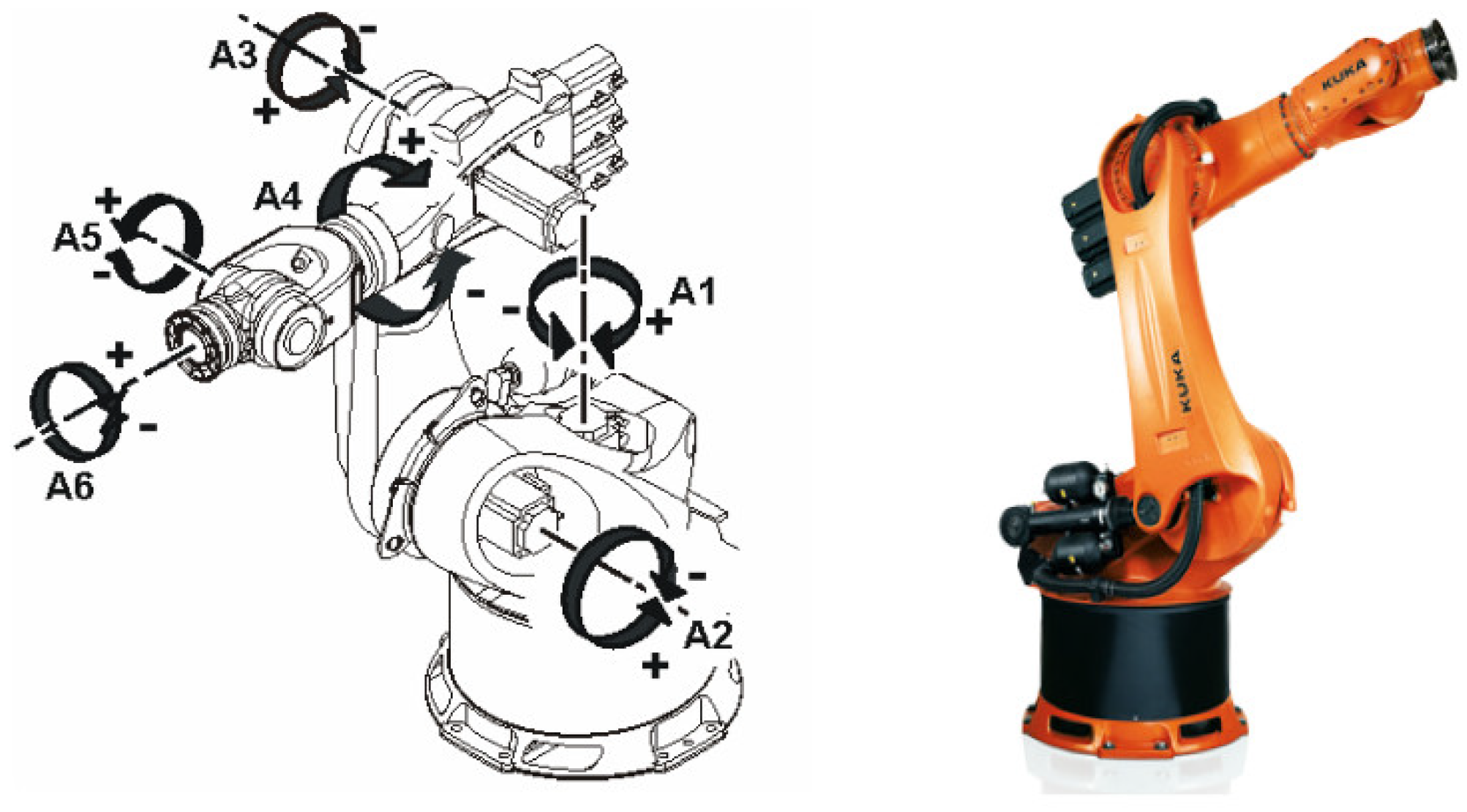
This paper selects the most commonly used industrial robot—an industrial robot with six rotational DOFs (6R robot system)—as the research object. The 6R robot system is composed of six rigid bodies and has six rotational DOFs, as shown in Figure 1. In this paper, a three-dimensional dynamic model of the 6R robot system is established based on graph theory. On this basis, a new method of dynamic parameter identification is proposed. A simulation experiment is designed by ADAMS software. The experimental results show that the result of parameter identification is extremely accurate and the dynamic model is accurate enough for the mathematical description of the 6R robot system. This proves the correctness and applicability of the dynamic theory and method used in this article. The 6R robot dynamics modeling theory and method proposed in this paper can realize the accurate 3D dynamic modeling of the 6R robot system. At present, there are very few studies in this area, so our exploratory research is very meaningful. At the same time, we propose for the first time a 6R robot dynamic parameter identification algorithm. The dynamic parameters obtained by this algorithm have extremely high precision, which is a meaningful innovation. The 6R robot dynamics modeling theory and method proposed in this paper can be used as the theoretical basis for precision manufacturing and precise control and it is of great significance to improve the automation and production efficiency of the manufacturing industry.

The rest of this paper is organized as follows. Section 2 introduces the dynamic modeling method and dynamic parameter identification method of the 6R robot system. In Section 3, an ADAMS simulation experiment is designed. The dynamic parameters and Lagrange multipliers of the 6R robot system are obtained by the calculation and identification of the experimental data and the calculation results are analyzed and discussed. Section 4 gives conclusions.

2. Dynamic Modeling of 6R Robot System

The 6R robot system consists of six rigid bodies (including the end effector) and six revolute joints, each rigid body has six DOF when it is unconstrained, that is, three DOF for movement and three DOF for rotation. The inside joint of a rigid body imposes five constraints on the rigid body, including three movement constraints and two rotation constraints and the constrained single rigid body has one rotational DOF. By extension, the unconstrained 6R robot system has a total of 36 DOF for the six rigid bodies and a total of 30 constraints provided by the six revolute joints, so that the constrained 6R robot system has a total of six rotational DOFs. That is, the number of DOF of the unconstrained 6R robot system minus the number of constraints on the system is equal to the number of DOF of the system.

First, the mathematical description of the 6R robot is defined based on graph theory and then the dynamic equations of the unconstrained 6R robot system are established. Taking a single rigid body as the object of study, the active force of the joint is regarded as the joint force element and the joint force element and gravity are the external forces on the rigid body. The virtual power principle is used to establish the kinetic equations for a single rigid body. The dynamic equations of the six rigid bodies are combined into a matrix form, that is, the dynamic equations of the unconstrained 6R robot system. Here, by rewriting the dynamic equation of the unconstrained 6R robot system, the mass and the principal moment of inertias of the rigid body are separated as the dynamic parameters to be identified, and we identified the dynamical parameters of the 6R robot system by using least squares method.

Second, the revolute joints provide five scleronomic and holonomic constraints (A constraint that restricts only the pose and does not contain time is called a scleronomic and holonomic constraint) on the outside connecting body, thereby the constraint equations of a single rigid body are established. The constraint equations of the six rigid bodies are combined to form the constraint equations of the 6R robot system.

Finally, the constrained equations of the 6R robot system are twice derived with respect to time and changed into the second-order derivative form in generalized coordinates, The Lagrange multiplier method is then used to combine the constraint equations with the dynamics equation of the unconstrained 6R robot system to become the dynamics equation of the constrained 6R robot system.

2.1. Graphical Description of the 6R Robot System

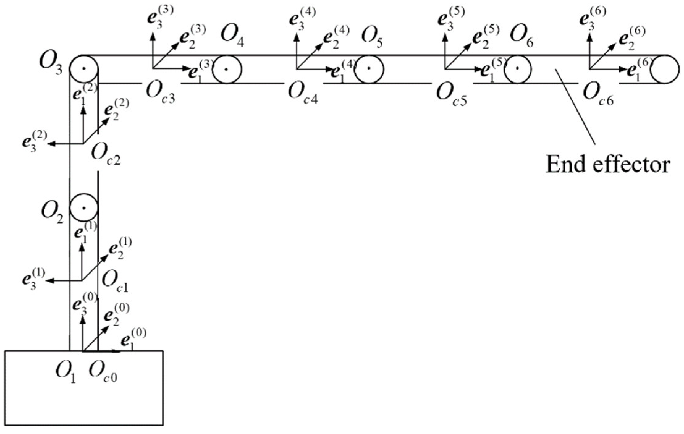
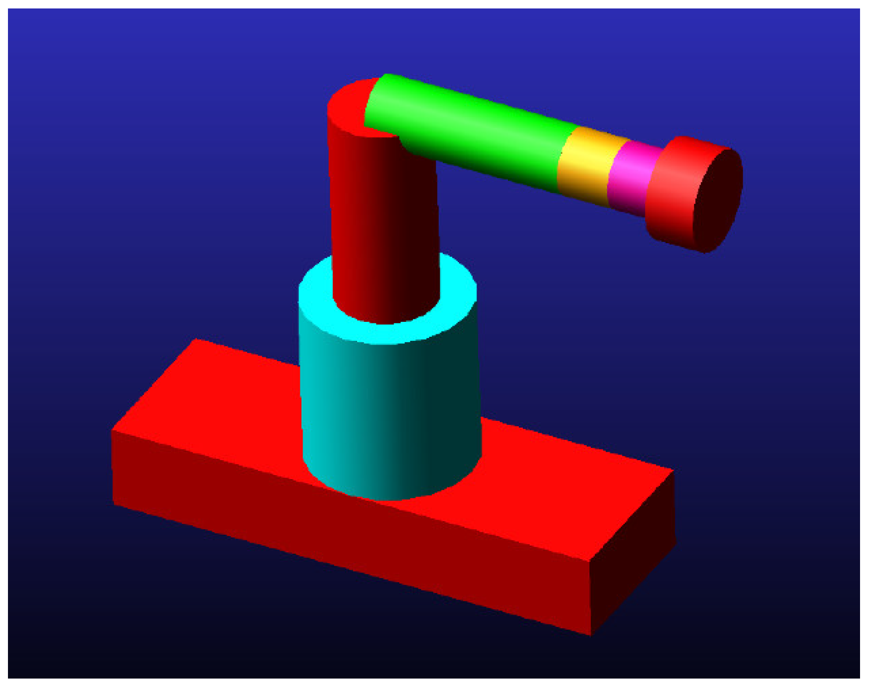
The six rigid bodies that make up the 6R robot system are simply represented as homogeneous cylinders, denoted as $B_i (i=1,2,\cdots ,6)$, the length of $B_i$ is denoted as $l_i$ and the radius is denoted as $R_i$, the center of mass of each rigid body is its geometric center, denoted as $O_{ci}(i=1,2,\cdots ,6)$. Establish the body-fixed base of each rigid body at the center of mass of each rigid body, denoted as $(O_i,{\underset{¯}{\mathit{e}}}^{(i)})(i=1,2,\cdots ,6)$ (The underscore $\underset{¯}{}$ indicates the matrix form), the three vectors ${\mathit{e}}_1^{(i)}$, ${\mathit{e}}_2^{(i)}$ and ${\mathit{e}}_3^{(i)}$ are the base vectors for each coordinate axis, the base vectors point to the direction of the central principal inertia axes. The body-fixed bases of the 6R robot system are shown in Figure 2, with the pose shown as the initial pose, the ${\mathit{e}}_1^{(i)}$ axis points from the inside to the outside along the length of the rigid body, the ${\mathit{e}}_2^{(i)}$ axis direction is perpendicular to the paper surface inwards and the ${\mathit{e}}_3^{(i)}$ axis direction is determined by the right-hand rule.

Since $B_0$ is firmly connected to the ground, in order to simplify the model and facilitate calculations, its volume and mass are both considered to be 0, its body-fixed base is $(O_0,{\underset{¯}{\mathit{e}}}^{(0)})$, which is located at $O_1$, $(O_0,{\underset{¯}{\mathit{e}}}^{(0)})$ is used as a fixed reference base and $O_0$ is used as a fixed reference point for this paper, the position of each center of mass is expressed relative to $O_0$ and the posture of each rigid body is expressed relative to $(O_0,{\underset{¯}{\mathit{e}}}^{(0)})$. The remaining rigid bodies are $B_1,B_2,\cdots ,B_6$ in the direction from $B_0$ to the end-effector, the body-fixed bases are $(O_1,{\underset{¯}{\mathit{e}}}^{(1)}),(O_2,{\underset{¯}{\mathit{e}}}^{(2)}),\cdots ,(O_6,{\underset{¯}{\mathit{e}}}^{(6)})$, the joint points are $O_1,O_2,\cdots ,O_6$ and the center of mass is $O_{c1},O_{c2},\cdots ,O_{c6}$ in that order.

The generalized coordinates of $B_i$ are determined by the Cartesian coordinates $x_i,y_i,z_i$ of $O_{ci}$ with respect to $O_0$ and the Cardano angles ${\alpha }_i,{\beta }_i,{\gamma }_i$ of $(O_i,{\underset{¯}{\mathit{e}}}^{(i)})$ with respect to $(O_0,{\underset{¯}{\mathit{e}}}^{(0)})$.

The pose of $B_i$ is recorded in the form of a coordinate matrix as:

$${\underset{¯}{r}}_i={(x_i y_i z_i)}^{\mathrm{T}},{\underset{¯}{\theta }}_i={({\alpha }_i {\beta }_i {\gamma }_i)}^{\mathrm{T}}.$$

(1)

$${\underset{¯}{q}}_i={({\underset{¯}{r}}_i {\underset{¯}{\theta }}_i)}^{\mathrm{T}}={(x_i y_i z_i {\alpha }_i {\beta }_i {\gamma }_i)}^{\mathrm{T}}.$$

(2)

where ${\underset{¯}{r}}_i$ is the position coordinate of $B_i$, ${\underset{¯}{\theta }}_i$ is the angular coordinate of $B_i$ and the combination of the two, ${\underset{¯}{q}}_i$, is the generalized coordinate of $B_i$. The generalized velocity column matrix and the generalized acceleration column matrix of $B_i$ are obtained by deriving:

$${\underset{¯}{\dot{r}}}_i={({\dot{x}}_i {\dot{y}}_i {\dot{z}}_i)}^{\mathrm{T}},{\underset{¯}{\dot{\theta }}}_i={({\dot{\alpha }}_i {\dot{\beta }}_i {\dot{\gamma }}_i)}^{\mathrm{T}}.$$

(3)

$${\underset{¯}{\ddot{r}}}_i={({\ddot{x}}_i {\ddot{y}}_i {\ddot{z}}_i)}^{\mathrm{T}},{\underset{¯}{\ddot{\theta }}}_i={({\ddot{\alpha }}_i {\ddot{\beta }}_i {\ddot{\gamma }}_i)}^{\mathrm{T}}.$$

(4)

$${\underset{¯}{\dot{q}}}_i={({\dot{x}}_i {\dot{y}}_i {\dot{z}}_i {\dot{\alpha }}_i {\dot{\beta }}_i {\dot{\gamma }}_i)}^{\mathrm{T}}.$$

(5)

$${\underset{¯}{q}}_i={({\underset{¯}{r}}_i {\underset{¯}{\theta }}_i)}^{\mathrm{T}}={(x_i y_i z_i {\alpha }_i {\beta }_i {\gamma }_i)}^{\mathrm{T}}.$$

(6)

The generalized coordinate column matrix of the multibody 6R robot system is composed of the coordinate column matrix of each single rigid body $B_i$ and expressed as a 36-dimensional coordinate column matrix:

$$\underset{¯}{q}={({\underset{¯}{q}}_1{}^{\mathrm{T}} {\underset{¯}{q}}_2{}^{\mathrm{T}} \cdots {\underset{¯}{q}}_6{}^{\mathrm{T}})}^{\mathrm{T}}={(q_1,q_2,\cdots ,q_{36})}^{\mathrm{T}}.$$

(7)

Some basic concepts of 6R robotics are defined according to graph theory:

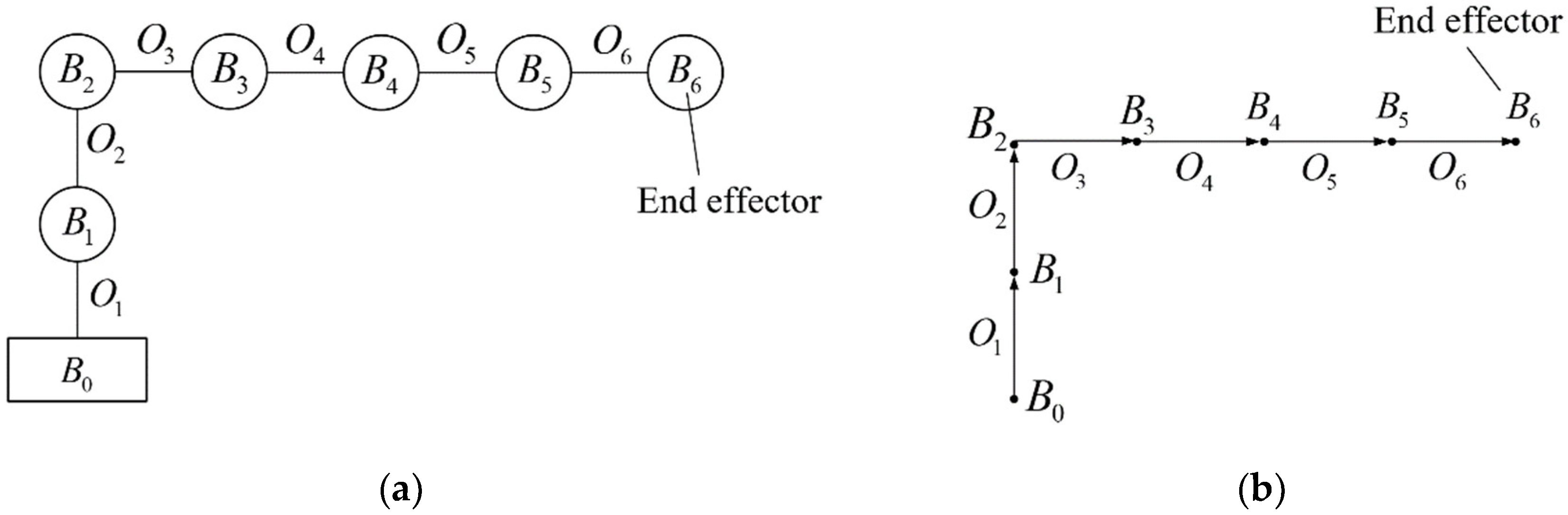
The relationship between a joint and a rigid body is called an incidence. A rigid body $B_i$ reaches $B_j$ via a series of rigid bodies and joints without repetition and the rigid bodies and joints $B_i$ passes through are called the path from $B_i$ to $B_j$. A system with only a unique path between any two joint points is called a system with tree structure. The system with tree structure and the structure diagram of the system with tree structure of the 6R robot system are shown in Figure 3.

If $B_j$ is on the path from $B_0$ to $B_i$, then $B_j$ is called the inside body of $B_i$ and $B_i$ is called the outside body of $B_i$. In particular, if the inside rigid body $B_j$ has incidence with $B_i$, then $B_j$ is called the inside connecting body of $B_i$ and the $O_i$ connecting $B_j$ and $B_i$ is called the inside joint of $B_i$. For $B_j$, $B_i$ is called the outside connecting body of $B_j$ and $O_i$ is called the outside joint of $B_j$.

Based on the above basic concepts, we established the incidence matrix, the matrix of body–joint vector, the path matrix of force element and the vector matrix of force element of the 6R robot system by graph theory, and deduced the resultant force and the resultant moment of the force element received by the rigid body.

First, the incidence matrix $\underset{\_}{S}$ of the 6R robot system is established.

Assuming that the robot system has $n$ rigid bodies, define an element:

$$S_{ij}=\left\{\begin{array}{cc}1& O_j \mathrm{has} \mathrm{incidence} \mathrm{with} B_i \mathrm{and} \mathrm{starts} \mathrm{with} B_i\\ -1& O_j \mathrm{has} \mathrm{incidence} \mathrm{with} B_i \mathrm{and} \mathrm{ends} \mathrm{with} B_i\\ 0& O_j \mathrm{has} \mathrm{no} \mathrm{incidence} \mathrm{with} B_i\end{array}\right. \left(i,j=1,2,\cdots ,n\right).$$

(8)

The $n\times n$ square matrix composed of $S_{ij}$ is called the incidence matrix of the system, denoted as $\underset{\_}{S}$.

$$\underset{¯}{S}=\left[\begin{array}{ccc}{S}_{11}& \cdots & S_{1n}\\ ⋮& \ddots & ⋮\\ S_{n1}& \cdots & S_{nn}\end{array}\right].$$

(9)

For the 6R robot system,

$$\underset{¯}{S}=\left[\begin{array}{cccccc}-1& 1& 0& 0& 0& 0\\ 0& -1& 1& 0& 0& 0\\ 0& 0& -1& 1& 0& 0\\ 0& 0& 0& -1& 1& 0\\ 0& 0& 0& 0& -1& 1\\ 0& 0& 0& 0& 0& -1\end{array}\right].$$

(10)

Second, the matrix of body–joint vector $\underset{\_}{\mathit{C}}$ of the 6R robot system is established.

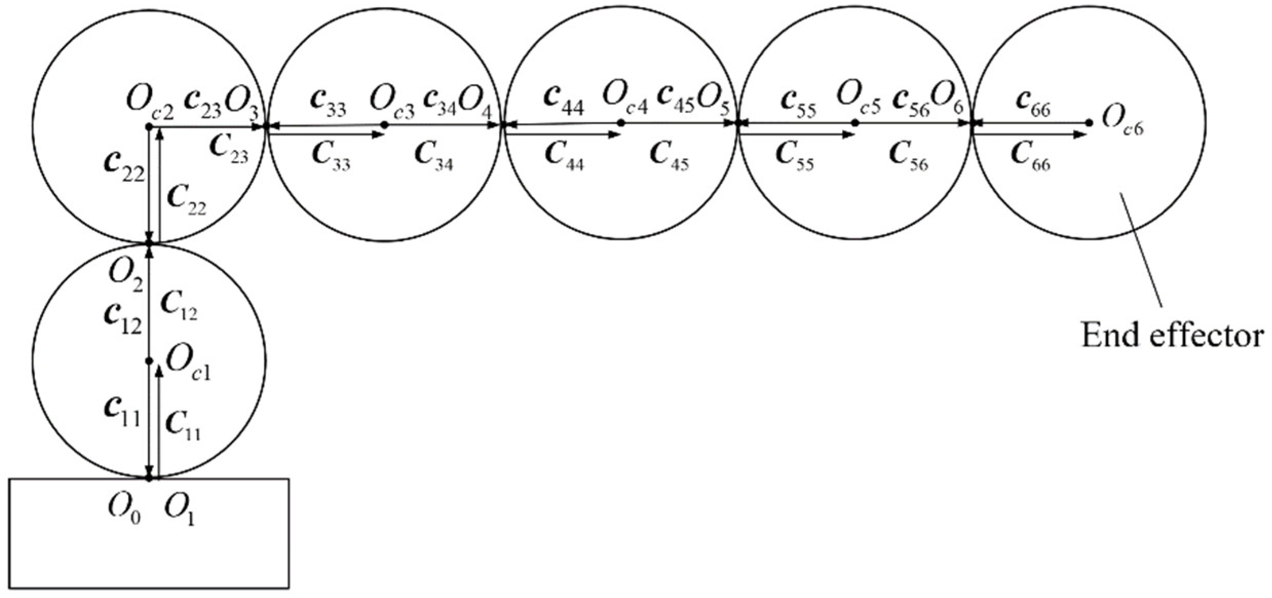
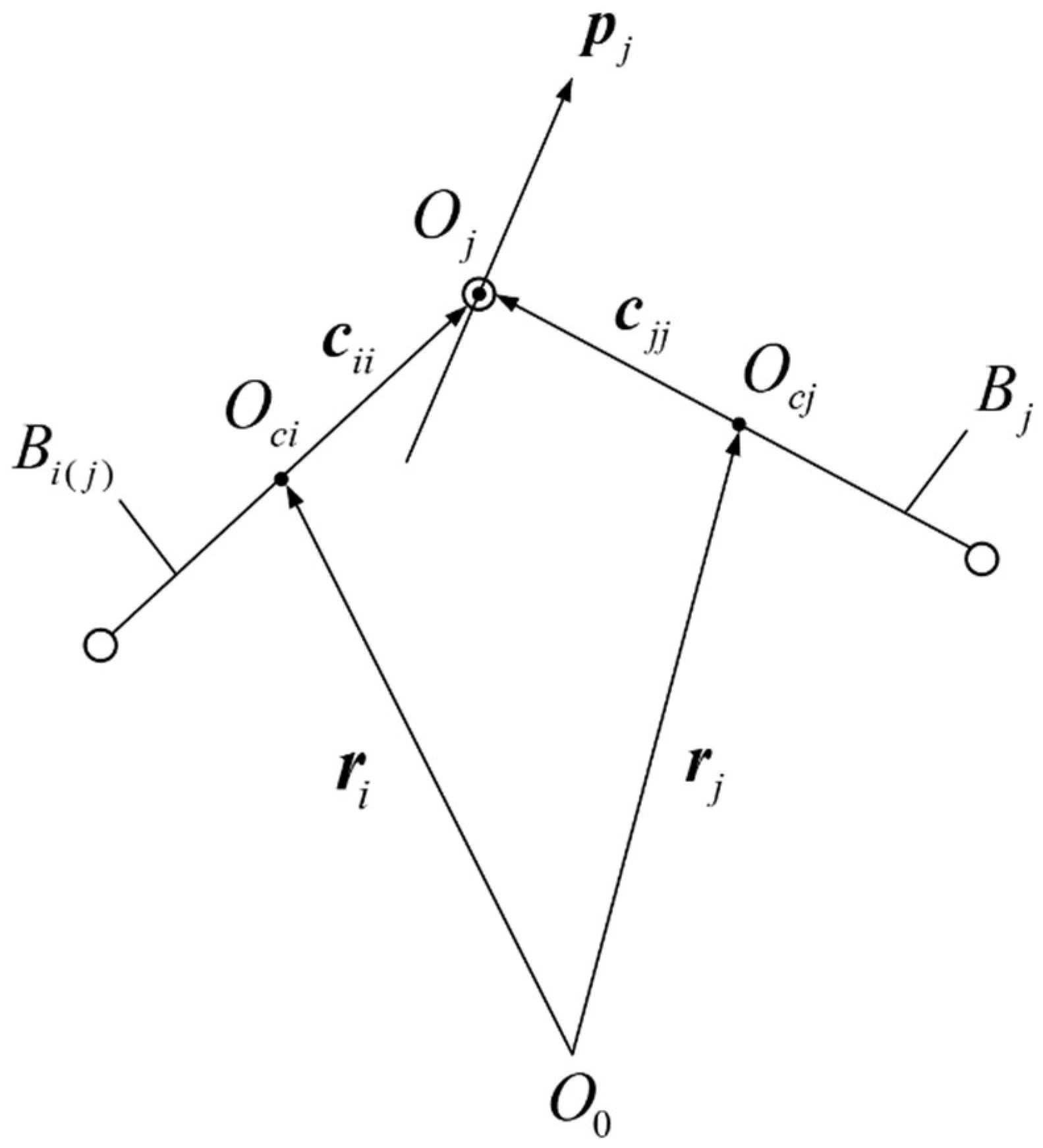
The vector pointing from $O_{ci}$ to any joint $O_j$ that has incidence with $B_j$$B_i$ is called the body–joint vector, denoted as ${\mathit{c}}_{ij}$. The multiplication of ${\mathit{c}}_{ij}$ and $S_{ij}$ is called the weighted body–joint vector, denoted as ${\mathit{C}}_{ij}$. The direction of ${\mathit{C}}_{ij}$ is away from $B_0$ and points to the outside. In particular, ${\mathit{c}}_{01}={\mathit{C}}_{01}=0$. The $n\times n$ square matrix composed of ${\mathit{C}}_{ij}$ is called the matrix of the body–joint vector of the system, denoted as $\underset{\_}{\mathit{C}}$. $\underset{\_}{\mathit{C}}$ reflects the distribution of joints that has incidence with the rigid bodies of the system.

For the 6R robot system,

$$\underset{¯}{\mathit{C}}=\left[\begin{array}{cccccc}\frac{l_1}{2}{\mathit{e}}_1^{(1)}& \frac{l_1}{2}{\mathit{e}}_1^{(1)}& 0& 0& 0& 0\\ 0& \frac{l_2}{2}{\mathit{e}}_1^{(2)}& \frac{l_2}{2}{\mathit{e}}_1^{(2)}& 0& 0& 0\\ 0& 0& \frac{l_3}{2}{\mathit{e}}_1^{(3)}& \frac{l_3}{2}{\mathit{e}}_1^{(3)}& 0& 0\\ 0& 0& 0& \frac{l_4}{2}{\mathit{e}}_1^{(4)}& \frac{l_4}{2}{\mathit{e}}_1^{(4)}& 0\\ 0& 0& 0& 0& \frac{l_5}{2}{\mathit{e}}_1^{(5)}& \frac{l_5}{2}{\mathit{e}}_1^{(5)}\\ 0& 0& 0& 0& 0& \frac{l_6}{2}{\mathit{e}}_1^{(6)}\end{array}\right].$$

(11)

The body-joint vector is shown in Figure 4.

The distribution of body-joint vectors of the 6R robot system is shown in Figure 5.

Third, the path matrix of force element for the 6R robot system is established and the resultant force of the force elements on the rigid body are derived.

The force element is the internal force doing work in the system, noted as $E_k$.

The force elements in this paper are only the joint force elements, that is, the active forces of the inside joint and the outside joint on the rigid body.

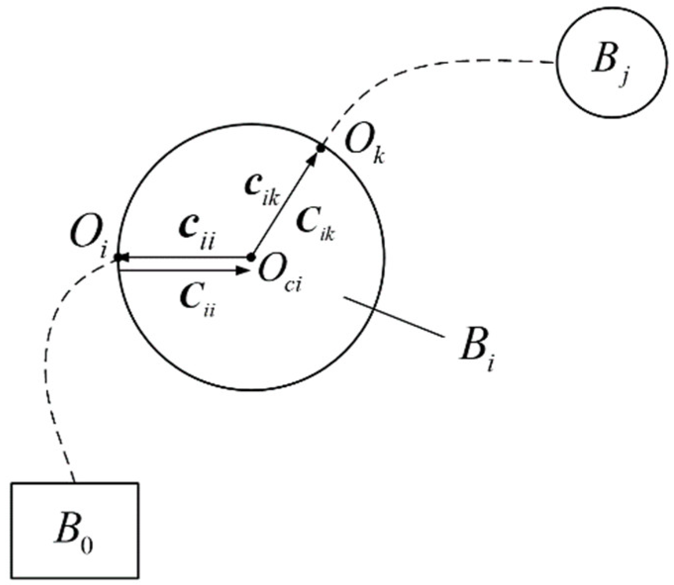
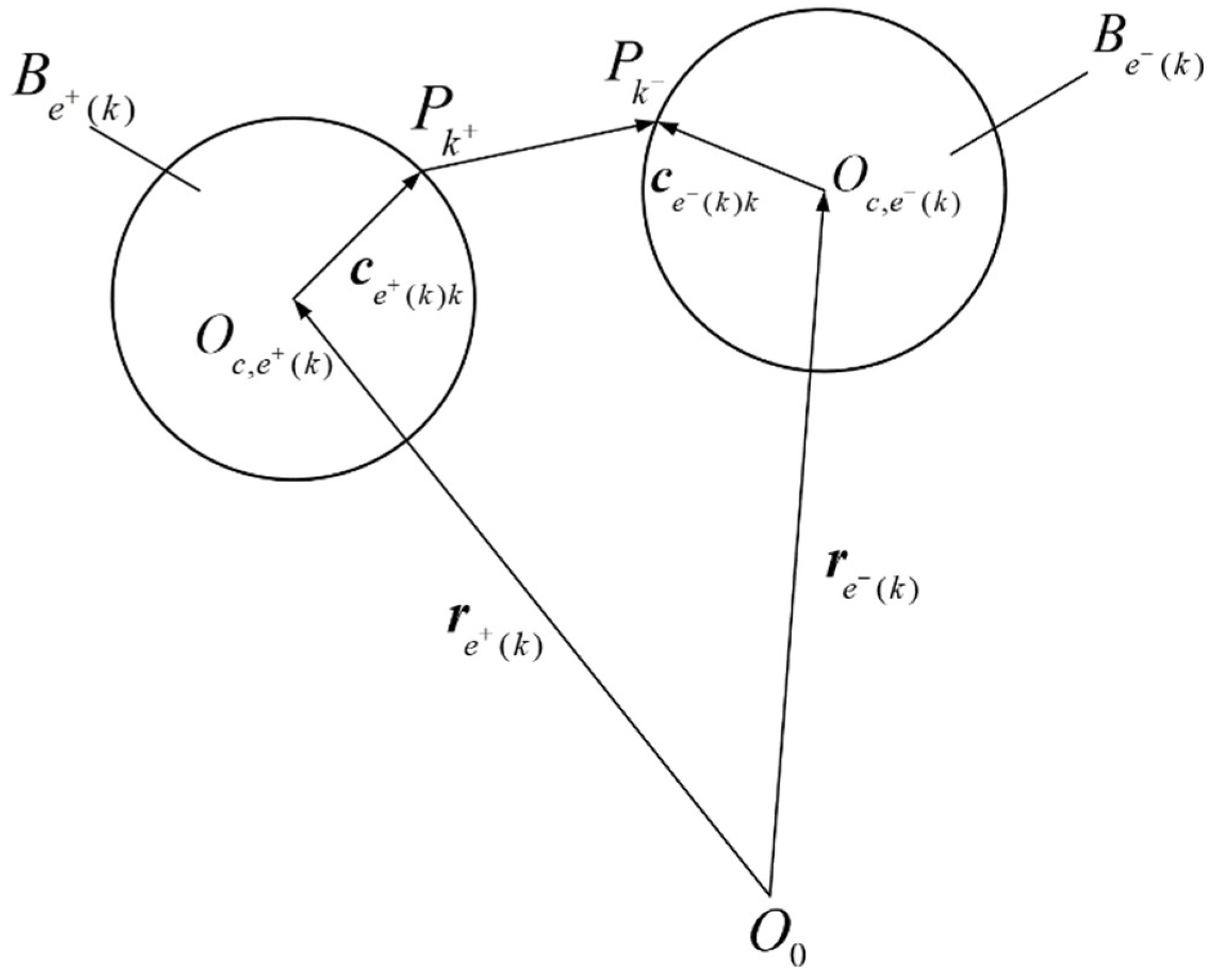
The $k$-th joint force element, $E_k$, has incidence with a pair of rigid bodies, the inside connecting body of the hinge is also called the inside connecting body of the force element and is denoted as $B_{e^{+}(k)}$. The outside connecting body of the joint is also called the outside connecting body of the force element and is denoted as $B_{e^{-}(k)}$. The points of action of $E_k$ on the outside connecting body and outside connecting body are noted as $P_k^{+}$ and $P_k^{-}$, respectively. As shown in Figure 6. The force of $E_k$ on a body is denoted as ${\mathit{F}}_k^e \left(k=1,2,\cdots ,n_e\right)$. The force ${\mathit{F}}_k^e$ of $B_{e^{+}(k)}$ on $B_{e^{-}(k)}$ points from $P_k^{+}$ to $P_k^{-}$ and the force $-{\mathit{F}}_k^e$ of $B_{e^{-}(k)}$ on $B_{e^{+}(k)}$ points from $P_k^{-}$ to $P_k^{+}$.

Assuming that the robot system has $n_e$ force elements, define an element:

$$S_{ik}^e=\left\{\begin{array}{cc}1& P_k^{+} \mathrm{has} \mathrm{incidence} \mathrm{with} B_i \\ -1& P_k^{-} \mathrm{has} \mathrm{incidence} \mathrm{with} B_i\\ 0& B_i \mathrm{has} \mathrm{no} \mathrm{incidence} \mathrm{with} P_k^{+} \mathrm{or} P_k^{-}\end{array}\right. \left(\begin{array}{c}i=1,2,\cdots ,n\\ k=1,2,\cdots ,n_e\end{array}\right).$$

(12)

The $n\times n_e$ square matrix composed of $S_{ik}^e$ is called the path matrix of force element of the system, denoted as ${\underset{\_}{S}}^e$. For the 6R robot system,

$${\underset{¯}{S}}^e=\left[\begin{array}{cccccc}-1& 1& 0& 0& 0& 0\\ 0& -1& 1& 0& 0& 0\\ 0& 0& -1& 1& 0& 0\\ 0& 0& 0& -1& 1& 0\\ 0& 0& 0& 0& -1& 1\\ 0& 0& 0& 0& 0& -1\end{array}\right].$$

(13)

The resultant force of all the joint elements on $B_i$ is denoted as ${\mathit{F}}_i^{\widehat{e}} \left(i=1,2,\cdots ,n\right)$.

$${\mathit{F}}_i^{\widehat{e}}=-{\displaystyle \sum _{k=1}^{n_e}{S}_{ik}^e{\mathit{F}}_k^e \left(i=1,2,\cdots ,n\right)}.$$

(14)

The $n_e$-order vector column matrix ${\underset{\_}{\mathit{F}}}^e$ formed by ${\mathit{F}}_k^e \left(k=1,2,\cdots ,n_e\right)$ and the $n$-order vector column matrix ${\underset{\_}{\mathit{F}}}^{\widehat{e}}$ formed by ${\mathit{F}}_i^{\widehat{e}} \left(i=1,2,\cdots ,n\right)$ have the following relationship:

$${\underset{\_}{\mathit{F}}}^{\widehat{e}}=-{\underset{\_}{S}}^e{\underset{\_}{\mathit{F}}}^e.$$

(15)

For the 6R robot system,

$${\underset{¯}{\mathit{F}}}^{\widehat{e}}=\left[\begin{array}{c}{\mathit{F}}_1^{\widehat{e}}\\ {\mathit{F}}_2^{\widehat{e}}\\ {\mathit{F}}_3^{\widehat{e}}\\ {\mathit{F}}_4^{\widehat{e}}\\ {\mathit{F}}_5^{\widehat{e}}\\ {\mathit{F}}_6^{\widehat{e}}\end{array}\right]=\left[\begin{array}{c}{\mathit{F}}_1^e-{\mathit{F}}_2^e\\ {\mathit{F}}_2^e-{\mathit{F}}_3^e\\ {\mathit{F}}_3^e-{\mathit{F}}_4^e\\ {\mathit{F}}_4^e-{\mathit{F}}_5^e\\ {\mathit{F}}_5^e-{\mathit{F}}_6^e\\ {\mathit{F}}_6^e\end{array}\right].$$

(16)

Finally, the vector matrix of force element of the 6R robot system is established and the resultant moment of the force elements on the rigid body are derived.

The vectors pointing from the centers of mass of rigid bodies $B_{e^{+}(k)}$ and $B_{e^{-}(k)}$ to the action points $P_k^{+}$ and $P_k^{-}$ of $E_k$, respectively, are called force element vectors and are denoted as ${\mathit{c}}_{ik}^e \left(i=e^{+}(k) or e^{-}(k)\right)$.

The weighted force element vector is defined as:

$${\mathit{C}}_{ik}^e=S_{ik}^e{\mathit{c}}_{ik}^e \left(\begin{array}{c}i=1,2,\cdots ,n\\ k=1,2,\cdots ,n_e\end{array}\right).$$

(17)

$C_{ik}^e$ that has incidence with $B_i$ is directed from the inside to the outside, and ${\mathit{C}}_{ik}^e$ that has no incidence with $B_i$ is zero.

The $n\times n_e$ square matrix composed of ${\mathit{C}}_{ik}^e$ is called the vector matrix of force element of the system, denoted as ${\underset{\_}{\mathit{C}}}^e$. ${\underset{\_}{\mathit{C}}}^e$ is used to describe the distribution of force elements in each rigid body of the system. For the 6R robot system,

$${\underset{¯}{\mathit{C}}}^e=\left[\begin{array}{cccccc}\frac{l_1}{2}{\mathit{e}}_1^{(1)}& \frac{l_1}{2}{\mathit{e}}_1^{(1)}& 0& 0& 0& 0\\ 0& \frac{l_2}{2}{\mathit{e}}_1^{(2)}& \frac{l_2}{2}{\mathit{e}}_1^{(2)}& 0& 0& 0\\ 0& 0& \frac{l_3}{2}{\mathit{e}}_1^{(3)}& \frac{l_3}{2}{\mathit{e}}_1^{(3)}& 0& 0\\ 0& 0& 0& \frac{l_4}{2}{\mathit{e}}_1^{(4)}& \frac{l_4}{2}{\mathit{e}}_1^{(4)}& 0\\ 0& 0& 0& 0& \frac{l_5}{2}{\mathit{e}}_1^{(5)}& \frac{l_5}{2}{\mathit{e}}_1^{(5)}\\ 0& 0& 0& 0& 0& \frac{l_6}{2}{\mathit{e}}_1^{(6)}\end{array}\right].$$

(18)

Therefore, the moment ${\mathit{M}}_i^{\widehat{e}} \left(i=1,2,\cdots ,n\right)$ of the force element that has incidence with $B_i$ to the center of mass $O_{ci}$ is expressed as:

$${\mathit{M}}_i^{\widehat{e}} =-{\displaystyle \sum _{k=1}^{n_e}{\mathit{C}}_{ik}^e\times {\mathit{F}}_k^e \left(i=1,2,\cdots ,n\right)}.$$

(19)

For the 6R robot system,

$${\underset{¯}{\mathit{M}}}_{}^{\widehat{e}}=-{\underset{¯}{\mathit{C}}}^e\times {\underset{¯}{\mathit{F}}}^e=\left[\begin{array}{c}({\mathit{F}}_1^e+{\mathit{F}}_2^e)\times \frac{l_1}{2}{\mathit{e}}_1^{(1)}\\ ({\mathit{F}}_2^e+{\mathit{F}}_3^e)\times \frac{l_2}{2}{\mathit{e}}_1^{(2)}\\ ({\mathit{F}}_3^e+{\mathit{F}}_4^e)\times \frac{l_3}{2}{\mathit{e}}_1^{(3)}\\ ({\mathit{F}}_4^e+{\mathit{F}}_5^e)\times \frac{l_4}{2}{\mathit{e}}_1^{(4)}\\ ({\mathit{F}}_5^e+{\mathit{F}}_6^e)\times \frac{l_5}{2}{\mathit{e}}_1^{(5)}\\ ({\mathit{F}}_6^e)\times \frac{l_6}{2}{\mathit{e}}_1^{(6)}\end{array}\right].$$

(20)

${\underset{¯}{\mathit{M}}}_{}^{\widehat{e}}={\left[\begin{array}{cccccc}{\mathit{M}}_1^{\widehat{e}} & {\mathit{M}}_2^{\widehat{e}}& {\mathit{M}}_3^{\widehat{e}}& {\mathit{M}}_4^{\widehat{e}}& {\mathit{M}}_5^{\widehat{e}}& {\mathit{M}}_6^{\widehat{e}}\end{array}\right]}^{\mathrm{T}}$ is the column matrix composed of ${\mathit{M}}_i^{\widehat{e}} \left(i=1,2,\cdots ,6\right)$.

2.2. Dynamical Modeling of Unconstrained 6R Robot System

The vector of $O_{ci}$ relative to $O_0$ is denoted as ${\mathit{r}}_i$, the angular velocity of $B_i$ relative to $(O_0,{\underset{¯}{\mathit{e}}}^{(0)})$ is denoted as ${\omega }_i$, the mass and central inertia tensor of $B_i$ are denoted as $m_i$ and $J_i$, respectively, and each component ${\mathit{e}}_1^{(i)},{\mathit{e}}_2^{(i)},{\mathit{e}}_3^{(i)}$ of $(O_i,{\underset{¯}{\mathit{e}}}^{(i)})$ is the central principal inertia axes of $B_i$. Equating each rigid body to a homogeneous cylinder, the central inertia tensor of each rigid body is expressed as:

$${\underset{¯}{J}}_i^{(i)}=\left[\begin{array}{ccc}{J}_{i_{11}}^{(i)}& 0& 0\\ 0& J_{i_{22}}^{(i)}& 0\\ 0& 0& J_{i_{33}}^{(i)}\end{array}\right]=\left[\begin{array}{ccc}\frac{1}{2}{m}_i{R}_i^2& 0& 0\\ 0& \frac{1}{12}{m}_i(3R_i^2+l_i^2)& 0\\ 0& 0& \frac{1}{12}{m}_i(3R_i^2+l_i^2)\end{array}\right].$$

(21)

The right-hand superscript ${}^{(i)}$ indicates an expression in $(O_i,{\underset{¯}{\mathit{e}}}^{(i)})$ and no right-hand superscript is an expression in $(O_0,{\underset{¯}{\mathit{e}}}^{(0)})$. $J_{i_{11}}^{(i)},J_{i_{22}}^{(i)},J_{i_{33}}^{(i)}$ are the three principal moments of inertia.

The Newton-Euler equations are derived by the principle of virtual power as follows:

$$m_i{\ddot{\mathit{r}}}_i={\mathit{F}}_i (i=1,2,\cdots ,6).$$

(22)

$${\mathit{J}}_i\cdot {\dot{\mathit{\omega }}}_i+{\mathit{\omega }}_i\times ({\mathit{J}}_i\cdot {\mathit{\omega }}_i)={\mathit{M}}_i (i=1,2,\cdots ,6).$$

(23)

Here,

$${\mathit{F}}_i={\mathit{F}}_i^g-{\mathit{F}}_i^{\widehat{e}}={\mathit{F}}_i^g-{\displaystyle \sum _{k=1}^{n_e}{S}_{ik}^e}{\mathit{F}}_k^e.$$

(24)

$${\mathit{M}}_i={\mathit{M}}_i^{\widehat{e}}+{\mathit{M}}_i^{\widehat{a}}=-{\displaystyle \sum _{k=1}^{n_e}({\mathit{C}}_{ik}^e\times {\mathit{F}}_k^e}+{\mathit{S}}_{ik}^{}\times {\mathit{M}}_k^a).$$

(25)

${\mathit{F}}_i^g$ is the gravity of $B_i$, ${\mathit{M}}_i^a$ is the active moment of $O_i$ on $B_i$, ${\mathit{M}}_i^{\widehat{a}}=-{\mathit{S}}_{ik}^{}\times {\mathit{M}}_k^a$${\mathit{M}}_i^{\widehat{a}}=-{\displaystyle \sum _{k=1}^{n_e}{\mathit{S}}_{ik}^{}\times {\mathit{M}}_k^a}$ is the active resultant moment of the joints that has incidence with $B_i$ on $B_i$.

For the 6R robot system,

$${\underset{¯}{\mathit{M}}}_{}^{\widehat{a}}=-\underset{¯}{\mathit{S}}\times {\underset{¯}{\mathit{M}}}_{}^a=\left[\begin{array}{c}{\mathit{M}}_1^a-{\mathit{M}}_2^a\\ {\mathit{M}}_2^a-{\mathit{M}}_3^a\\ {\mathit{M}}_3^a-{\mathit{M}}_4^a\\ {\mathit{M}}_4^a-{\mathit{M}}_5^a\\ {\mathit{M}}_5^a-{\mathit{M}}_6^a\\ {\mathit{M}}_6^a\end{array}\right].$$

(26)

${\underset{¯}{\mathit{M}}}_{}^a={\left[\begin{array}{cccccc}{\mathit{M}}_1^a & {\mathit{M}}_2^a & {\mathit{M}}_3^a & {\mathit{M}}_4^a & {\mathit{M}}_5^a & {\mathit{M}}_6^a \end{array}\right]}^{\mathrm{T}}$ is the column matrix composed of ${\mathit{M}}_i^a \left(i=1,2,\cdots ,6\right)$.

Therefore, for the 6R robotics system,

$$\underset{¯}{\mathit{M}}={\mathit{M}}_{}^{\widehat{e}}+{\mathit{M}}_{}^{\widehat{a}}=\left[\begin{array}{c}({\mathit{F}}_1^e+{\mathit{F}}_2^e)\times \frac{l_1}{2}{\mathit{e}}_1^{(1)}\\ ({\mathit{F}}_2^e+{\mathit{F}}_3^e)\times \frac{l_2}{2}{\mathit{e}}_1^{(2)}\\ ({\mathit{F}}_3^e+{\mathit{F}}_4^e)\times \frac{l_3}{2}{\mathit{e}}_1^{(3)}\\ ({\mathit{F}}_4^e+{\mathit{F}}_5^e)\times \frac{l_4}{2}{\mathit{e}}_1^{(4)}\\ ({\mathit{F}}_5^e+{\mathit{F}}_6^e)\times \frac{l_5}{2}{\mathit{e}}_1^{(5)}\\ ({\mathit{F}}_6^e)\times \frac{l_6}{2}{\mathit{e}}_1^{(6)}\end{array}\right]+\left[\begin{array}{c}{\mathit{M}}_1^a-{\mathit{M}}_2^a\\ {\mathit{M}}_2^a-{\mathit{M}}_3^a\\ {\mathit{M}}_3^a-{\mathit{M}}_4^a\\ {\mathit{M}}_4^a-{\mathit{M}}_5^a\\ {\mathit{M}}_5^a-{\mathit{M}}_6^a\\ {\mathit{M}}_6^a\end{array}\right].$$

(27)

$\underset{¯}{\mathit{M}}={\left[\begin{array}{cccccc}{\mathit{M}}_1^{} & {\mathit{M}}_2^{} & {\mathit{M}}_3^{} & {\mathit{M}}_4^{} & {\mathit{M}}_5^{} & {\mathit{M}}_6^{} \end{array}\right]}^{\mathrm{T}}$ is the column matrix composed of ${\mathit{M}}_i^{} \left(i=1,2,\cdots ,6\right)$.

We call Equation (22) the center of mass motion equation and Equation (23) the posture motion equation. Both equations need to be expressed in the form of a matrix of generalized coordinates.

First, the center of mass motion equation, Equation (22), is written in matrix form:

$$m_i{\underset{¯}{\ddot{r}}}_i={\underset{¯}{A}}^{(0i)}{\underset{¯}{F}}_i^{(i)}={\underset{¯}{F}}_i^{} (i=1,2,\cdots ,6).$$

(28)

${\underset{¯}{A}}^{(0i)}$ is the coordinate transformation matrix expressed by Cardano angles.

$${\underset{¯}{A}}^{(0i)}=\left[\begin{array}{ccc}c{\beta }_{i}c{\gamma }_i& -c{\beta }_{i}s{\gamma }_i& s{\beta }_i\\ c{\alpha }_{i}s{\gamma }_i+s{\alpha }_{i}s{\beta }_{i}c{\gamma }_i& c{\alpha }_{i}c{\gamma }_i-s{\alpha }_{i}s{\beta }_{i}s{\gamma }_i& -s{\alpha }_{i}c{\beta }_i\\ s{\alpha }_{i}s{\gamma }_i-c{\alpha }_{i}s{\beta }_{i}c{\gamma }_i& s{\alpha }_{i}c{\gamma }_i+c{\alpha }_{i}s{\beta }_{i}s{\gamma }_i& c{\alpha }_{i}c{\beta }_i\end{array}\right].$$

(29)

Then, the posture motion equation, Equation (23), is expressed in matrix form relative to $(O_i,{\underset{¯}{\mathit{e}}}^{(i)})$ as:

$${\underset{¯}{J}}_i^{(i)}{\underset{¯}{\dot{\omega }}}_i^{(i)}+{\underset{¯}{\tilde{\omega }}}_i^{(i)}{\underset{¯}{J}}_i^{(i)}{\underset{¯}{\omega }}_i^{(i)}={\underset{¯}{M}}_i^{(i)} (i=1,2,\cdots ,6).$$

(30)

Here, the matrix symbol $\underset{¯}{\tilde{a}}$ with tilde denotes the following three-order antisymmetric matrix:

$$\underset{¯}{\tilde{a}}=\left[\begin{array}{ccc}0& -a_3& a_2\\ a_3& 0& -a_1\\ -a_2& a_1& 0\end{array}\right].$$

(31)

Express posture motion equation, Equation (30), by generalized angular coordinates as follows:

$${\underset{¯}{J}}_i^{(i)}{\underset{¯}{D}}_i{\underset{¯}{\ddot{\mathit{\theta }}}}_i+({\underset{¯}{J}}_i^{(i)}{\underset{¯}{\dot{D}}}_i+\tilde{{\underset{¯}{D}}_i{\underset{¯}{\dot{\mathit{\theta }}}}_i}{\underset{¯}{J}}_i^{(i)}{\underset{¯}{D}}_i){\underset{¯}{\dot{\mathit{\theta }}}}_i={\underset{¯}{M}}_i^{(i)} (i=1,2,\cdots ,6).$$

(32)

Here,

$${\underset{¯}{D}}_i=\left[\begin{array}{ccc}c{\beta }_{i}c{\gamma }_i& s{\gamma }_i& 0\\ -c{\beta }_{i}s{\gamma }_i& c{\gamma }_i& 0\\ s{\beta }_i& 0& 1\end{array}\right] (i=1,2,\cdots ,6).$$

(33)

$${\underset{¯}{\dot{D}}}_i=\left[\begin{array}{ccc}-{\dot{\beta }}_{i}s{\beta }_{i}c{\gamma }_i-{\dot{\gamma }}_{i}c{\beta }_{i}s{\gamma }_i& {\dot{\gamma }}_{i}c{\gamma }_i& 0\\ {\dot{\beta }}_{i}s{\beta }_{i}s{\gamma }_i-{\dot{\gamma }}_{i}c{\beta }_{i}c{\gamma }_i& -{\dot{\gamma }}_{i}s{\gamma }_i& 0\\ {\dot{\beta }}_{i}c{\beta }_i& 0& 1\end{array}\right] (i=1,2,\cdots ,6).$$

(34)

The dynamic equation of the rigid body expressed by generalized coordinates is obtained by combining Equations (28) and (32) as follows:

$$\left[\begin{array}{cc}{m}_i\underset{¯}{E}& \underset{¯}{0}\\ \underset{¯}{0}& {\underset{¯}{J}}_i^{(i)}{\underset{¯}{D}}_i\end{array}\right]\left[\begin{array}{c}{\underset{¯}{\ddot{r}}}_i\\ {\underset{¯}{\ddot{\theta }}}_i\end{array}\right]=\left[\begin{array}{c}\underset{¯}{0}\\ -({\underset{¯}{J}}_i^{(i)}{\underset{¯}{\dot{D}}}_i+\tilde{{\underset{¯}{D}}_i{\underset{¯}{\dot{\theta }}}_i}{\underset{¯}{J}}_i^{(i)}{\underset{¯}{D}}_i){\underset{¯}{\dot{\theta }}}_i\end{array}\right]+\left[\begin{array}{c}{\underset{¯}{A}}^{(0i)}{\underset{¯}{F}}_i^{(i)}\\ {\underset{¯}{M}}_i^{(i)}\end{array}\right] (i=1,2,\cdots ,6).$$

(35)

Equation (35) is abbreviated as:

$${\underset{¯}{A}}_i{\underset{¯}{\ddot{q}}}_i={\underset{¯}{B}}_i (i=1,2,\cdots ,6).$$

(36)

Here,

$$\left.\begin{array}{l}{\underset{¯}{A}}_i=\left[\begin{array}{cc}{m}_i\underset{¯}{E}& \underset{¯}{0}\\ \underset{¯}{0}& {\underset{¯}{J}}_i^{(i)}{\underset{¯}{D}}_i\end{array}\right]\\ {\underset{¯}{B}}_i=\left[\begin{array}{c}{\underset{¯}{A}}^{(0i)}{\underset{¯}{F}}_i^{(i)}\\ -({\underset{¯}{J}}_i^{(i)}{\underset{¯}{\dot{D}}}_i+\tilde{{\underset{¯}{D}}_i{\underset{¯}{\dot{\theta }}}_i}{\underset{¯}{J}}_i^{(i)}{\underset{¯}{D}}_i){\underset{¯}{\dot{\theta }}}_i+{\underset{¯}{M}}_i^{(i)}\end{array}\right] \end{array}\right\} (i=1,2,\cdots ,6).$$

(37)

The dynamic equation for the unconstrained 6R robot system is derived as:

$$\underset{¯}{A}\underset{¯}{\ddot{q}}=\underset{¯}{B}.$$

(38)

Here,

$$\underset{¯}{A}=diag({\underset{¯}{A}}_1 \underset{¯}{A}{ }_2 \cdots {\underset{¯}{A}}_6), \underset{¯}{B}={({\underset{¯}{B}}_1^T {\underset{¯}{B}}_2^T \cdots {\underset{¯}{B}}_6^T)}^T.$$

(39)

$\underset{¯}{A}$ is a 36-order square matrix and $\underset{¯}{B}$ is a 36-order column matrix.

2.3. Dynamic Parameter Identification of 6R Robot System

The dynamic parameters of the 6R robot include the mass $m_i$ of each rigid body and the three principal moments of inertia $J_{i_{11}}^{(i)},J_{i_{22}}^{(i)},J_{i_{33}}^{(i)}$.

The force element ${\mathit{F}}_i{}^{(i)}$ exerted by each joint and the moment ${\mathit{M}}_i{}^{(i)}$ of the force element ${\mathit{F}}_i{}^{(i)}$ to the center of mass and the angular velocity and angular acceleration of each rigid body and the acceleration of the center of mass of each rigid body are regarded as known quantities, dynamic parameters are regarded to be unknown quantities. We rewrote the dynamic equation into parameter identification form and identified it by using the least squares method.

First, the center of mass motion equation Equation (22) is rewritten.

The expansion of ${\mathit{F}}_i$ in Equation (22) is written as:

$${\mathit{F}}_i={\mathit{F}}_i^g-{\displaystyle \sum _{k=1}^{n_e}{S}_{ik}^e}{\mathit{F}}_k^e=\left[\begin{array}{c}-{\displaystyle \sum _{k=1}^{n_e}{S}_{ik}^e}{F}_{k1}^e\\ -{\displaystyle \sum _{k=1}^{n_e}{S}_{ik}^e}{F}_{k2}^e\\ m_{i}g-{\displaystyle \sum _{k=1}^{n_e}{S}_{ik}^e}{F}_{k3}^e\end{array}\right].$$

(40)

Here, $F_{k1}^e$, $F_{k2}^e$ and $F_{k3}^e$ are the components of ${\mathit{F}}_k^e$ on ${\mathit{e}}_1^{(0)}$, ${\mathit{e}}_2^{(0)}$ and ${\mathit{e}}_3^{(0)}$ respectively.

The expansion of Equation (22) is written as:

$$m_i\left[\begin{array}{ccc}{\ddot{\mathit{x}}}_i& & \\ & {\ddot{\mathit{y}}}_i& \\ & & {\ddot{\mathit{z}}}_i\end{array}\right]=\left[\begin{array}{c}-{\displaystyle \sum _{k=1}^{n_e}{S}_{ik}^e}{\mathit{F}}_{k1}^e\\ -{\displaystyle \sum _{k=1}^{n_e}{S}_{ik}^e}{\mathit{F}}_{k2}^e\\ m_{i}g-{\displaystyle \sum _{k=1}^{n_e}{S}_{ik}^e}{\mathit{F}}_{k3}^e\end{array}\right] (i=1,2,\cdots ,6).$$

(41)

Since gravity ${\mathit{F}}_i^g$ is a function of the unknown quantity $m_i$ to be identified, move it to the left. Equation (41) is rewritten in parameter identification form as follows:

$$\left[\begin{array}{ccc}{\ddot{\mathit{x}}}_i& & \\ & {\ddot{\mathit{y}}}_i& \\ & & {\ddot{\mathit{z}}}_i-g\end{array}\right]\left[\begin{array}{c}{m}_i\\ m_i\\ m_i\end{array}\right]=\left[\begin{array}{c}-{\displaystyle \sum _{k=1}^{n_e}{S}_{ik}^e}{\mathit{F}}_{k1}^e\\ -{\displaystyle \sum _{k=1}^{n_e}{S}_{ik}^e}{\mathit{F}}_{k2}^e\\ -{\displaystyle \sum _{k=1}^{n_e}{S}_{ik}^e}{\mathit{F}}_{k3}^e\end{array}\right] (i=1,2,\cdots ,6).$$

(42)

Equation (42) is written in matrix form as follows:

$${}^{\mathit{id}}\underset{\_}{R}{}_i {}^{\mathit{id}}\underset{\_}{m}{}_i={\underset{¯}{F}}_i^R={\underset{¯}{A}}^{(0i)}{\underset{¯}{F}}_i^{R(i)} (i=1,2,\cdots ,6).$$

(43)

Here,

$${}^{\mathit{id}}\underset{\_}{R}{}_i=\left[\begin{array}{ccc}{\ddot{x}}_i& & \\ & {\ddot{y}}_i& \\ & & {\ddot{z}}_i+g\end{array}\right], {}^{\mathit{id}}\underset{\_}{m}{}_i=\left[\begin{array}{c}{m}_i\\ m_i\\ m_i\end{array}\right], {\underset{¯}{F}}_i^R=\left[\begin{array}{c}-{\displaystyle \sum _{k=1}^{n_e}{S}_{ik}^e}{F}_{k1}^e\\ -{\displaystyle \sum _{k=1}^{n_e}{S}_{ik}^e}{F}_{k2}^e\\ -{\displaystyle \sum _{k=1}^{n_e}{S}_{ik}^e}{F}_{k3}^e\end{array}\right].$$

(44)

Second, the posture motion equation, Equation (30), is rewritten. The expansion of Equation (30) is written as:

$$\left[\begin{array}{ccc}{J}_{i_{11}}^{(i)}& 0& 0\\ 0& J_{i_{22}}^{(i)}& 0\\ 0& 0& J_{i_{33}}^{(i)}\end{array}\right]\left[\begin{array}{c}{\dot{\omega }}_{i1}^{(i)}\\ {\dot{\omega }}_{i2}^{(i)}\\ {\dot{\omega }}_{i3}^{(i)}\end{array}\right] + \left[\begin{array}{ccc}0& -{\omega }_{i3}^{(i)}& {\omega }_{i2}^{(i)}\\ {\omega }_{i3}^{(i)}& 0& -{\omega }_{i1}^{(i)}\\ -{\omega }_{i2}^{(i)}& {\omega }_{i1}^{(i)}& 0\end{array}\right]\left[\begin{array}{ccc}{J}_{i_{11}}^{(i)}& 0& 0\\ 0& J_{i_{22}}^{(i)}& 0\\ 0& 0& J_{i_{33}}^{(i)}\end{array}\right]\left[\begin{array}{c}{\omega }_{i1}^{(i)}\\ {\omega }_{i2}^{(i)}\\ {\omega }_{i3}^{(i)}\end{array}\right]={\underset{¯}{M}}_i^{(i)}(i=1,2,\cdots ,6)$$

(45)

Here, ${\omega }_{i1}^{(i)}$, ${\omega }_{i2}^{(i)}$ and ${\omega }_{i3}^{(i)}$ are the components of ${\mathit{\omega }}^{(i)}$ on ${\mathit{e}}_1^{(i)}$, ${\mathit{e}}_2^{(i)}$ and ${\mathit{e}}_3^{(i)}$ respectively.

Equation (45) is rewritten in parameter identification form as follows:

$$\left[\begin{array}{ccc}{\dot{\omega }}_{i1}^{(i)}& -{\omega }_{i2}^{(i)}{\omega }_{i3}^{(i)}& {\omega }_{i2}^{(i)}{\omega }_{i3}^{(i)}\\ {\omega }_{i1}^{(i)}{\omega }_{i3}^{(i)}& {\dot{\omega }}_{i2}^{(i)}& -{\omega }_{i1}^{(i)}{\omega }_{i3}^{(i)}\\ -{\omega }_{i1}^{(i)}{\omega }_{i2}^{(i)}& {\omega }_{i1}^{(i)}{\omega }_{i2}^{(i)}& {\dot{\omega }}_{i3}^{(i)}\end{array}\right]\left[\begin{array}{c}{J}_{i_{11}}^{(i)}\\ J_{i_{22}}^{(i)}\\ J_{i_{33}}^{(i)}\end{array}\right]={\underset{¯}{M}}_i^{(i)} (i=1,2,\cdots ,6).$$

(46)

Equation (46) is abbreviated as the following form:

$${}^{id}{\underset{\_}{S}}_i^{(i)}{ }^{id}{\underset{¯}{J}}_i^{(i)}={\underset{¯}{M}}_i^{(i)} (i=1,2,\cdots ,6).$$

(47)

Here,

$${}^{id}{\underset{\_}{S}}_i^{(i)}=\left[\begin{array}{ccc}{\dot{\omega }}_{i1}^{(i)}& -{\omega }_{i2}^{(i)}{\omega }_{i3}^{(i)}& {\omega }_{i2}^{(i)}{\omega }_{i3}^{(i)}\\ {\omega }_{i1}^{(i)}{\omega }_{i3}^{(i)}& {\dot{\omega }}_{i2}^{(i)}& -{\omega }_{i1}^{(i)}{\omega }_{i3}^{(i)}\\ -{\omega }_{i1}^{(i)}{\omega }_{i2}^{(i)}& {\omega }_{i1}^{(i)}{\omega }_{i2}^{(i)}& {\dot{\omega }}_{i3}^{(i)}\end{array}\right], { }^{id}{\underset{¯}{J}}_i^{(i)}=\left[\begin{array}{c}{J}_{i_{11}}^{(i)}\\ J_{i_{22}}^{(i)}\\ J_{i_{33}}^{(i)}\end{array}\right] (i=1,2,\cdots ,6).$$

(48)

Finally, the rewritten center of mass motion equation, Equation (43), and the rewritten posture motion equation, Equation (47), are combined and expressed as the following form, that is, a dynamic equation with parameter identification form.

$$\left[\begin{array}{cc} {}^{\mathit{id}}\underset{\_}{R}{}_i& \\ & {}^{id}{\underset{\_}{S}}_i^{(i)}\end{array}\right]\left[\begin{array}{c} {}^{\mathit{id}}\underset{\_}{m}{}_i\\ {}^{\mathit{id}}\underset{¯}{J}{}_i^{(i)}\end{array}\right]=\left[\begin{array}{c}{\underset{¯}{A}}^{(0i)}{\underset{¯}{F}}_i^{R(i)}\\ {\underset{¯}{M}}_i^{(i)}\end{array}\right] (i=1,2,\cdots ,6).$$

(49)

Equation (49) is abbreviated as the following form:

$${}^{id}{\underset{\_}{Y}}_i {}^{\mathit{id}}\underset{\_}{X}{ }_i{=}^{id}{\underset{\_}{Z}}_i.$$

(50)

Here,

$${}^{id}{\underset{\_}{Y}}_i=\left[\begin{array}{cc} {}^{\mathit{id}}\underset{\_}{R}{}_i& \\ & {}^{id}{\underset{\_}{S}}_i^{(i)}\end{array}\right], { }^{id}{\underset{\_}{X}}_i=\left[\begin{array}{c} {}^{\mathit{id}}\underset{\_}{m}{}_i\\ {}^{\mathit{id}}\underset{¯}{J}{}_i^{(i)}\end{array}\right], { }^{id}{\underset{\_}{Z}}_i=\left[\begin{array}{c}{\underset{¯}{A}}^{(0i)}{\underset{¯}{F}}_i^{R(i)}\\ {\underset{¯}{M}}_i^{(i)}\end{array}\right].$$

(51)

This is the dynamic equation with the parameter identification form of $B_i$ and ${}^{id}{\underset{\_}{X}}_i$ is the dynamic parameter to be identified. ${}^{id}{\underset{\_}{Y}}_i$ and ${}^{id}{\underset{\_}{Z}}_i$ are known parameters obtained by sampling the system, sampling at multiple times to obtain multiple sets of data. The dynamic parameter ${}^{id}{\underset{\_}{X}}_i$ of the 6R robot system is identified by using the least squares method.

For time $t_j$, the dynamic equation with parameter identification form is expressed as:

$${}_j^{id}{\underset{\_}{Y}}_i= {}^{\mathit{id}}\underset{\_}{X}{}_i { }_j^{id}{\underset{\_}{Z}}_i.$$

(52)

Assuming that there are $n$ sets of data, that is, $1\le j\le n$, corresponding to times $t_j (j=1,2,\cdots ,n)$ respectively, then the following equation is formed.

$$\left[\begin{array}{c}{}_1^{id}{\underset{\_}{Y}}_i\\ {}_2^{id}{\underset{\_}{Y}}_i\\ ⋮\\ {}_n^{id}{\underset{\_}{Y}}_i\end{array}\right] {}^{\mathit{id}}\underset{\_}{X}{}_i=\left[\begin{array}{c}{}_1^{id}{\underset{\_}{Z}}_i\\ {}_2^{id}{\underset{\_}{Z}}_i\\ ⋮\\ {}_n^{id}{\underset{\_}{Z}}_i\end{array}\right].$$

(53)

Equation (53) is abbreviated as the following form:

$${}^{\mathit{id}}\underset{\_}{K}{}_i {}^{\mathit{id}}\underset{\_}{X}{}_i= {}^{\mathit{id}}\underset{\_}{L}{}_i.$$

(54)

Here,

$${}^{\mathit{id}}\underset{\_}{K}{}_i=\left[\begin{array}{c}{}_1^{id}{\underset{\_}{Y}}_i\\ {}_2^{id}{\underset{\_}{Y}}_i\\ ⋮\\ {}_n^{id}{\underset{\_}{Y}}_i\end{array}\right], {}^{\mathit{id}}\underset{\_}{L}{}_i=\left[\begin{array}{c}{}_1^{id}{\underset{\_}{Z}}_i\\ {}_2^{id}{\underset{\_}{Z}}_i\\ ⋮\\ {}_n^{id}{\underset{\_}{Z}}_i\end{array}\right].$$

(55)

Then the least squares solution of Equation (54) is:

$${}^{\mathit{id}}\underset{\_}{X} {}_i={( {}^{\mathit{id}}\underset{\_}{K} {{}_i}^{\mathrm{T}} {}^{\mathit{id}}\underset{\_}{K} {}_i)}^{-1} {}^{\mathit{id}}\underset{\_}{K}{{}_i}^{\mathrm{T}} {}^{\mathit{id}}\underset{\_}{L}{}_i.$$

(56)

This means that the dynamic parameters of the rigid body can be identified by using least squares method by sampling the acceleration of the center of mass and the angular velocity and angular acceleration and the data of the joint force element of the rigid body at multiple times.

The above is our method for identifying the dynamic parameters of a single rigid body, from which we can further derive a method for identifying the dynamic parameters of the 6R robot system.

The 6R robot system is a combination of rigid bodies, therefore the dynamic equation with parameter identification form is written as:

$$\left[\begin{array}{cccccc}{}^{id}{\underset{\_}{Y}}_1& & & & & \\ & {}^{id}{\underset{\_}{Y}}_2& & & & \\ & & {}^{id}{\underset{\_}{Y}}_3& & & \\ & & & {}^{id}{\underset{\_}{Y}}_4& & \\ & & & & {}^{id}{\underset{\_}{Y}}_5& \\ & & & & & {}^{id}{\underset{\_}{Y}}_6\end{array}\right]\left[\begin{array}{c} {}^{\mathit{id}}\underset{\_}{X}{ }_1\\ {}^{\mathit{id}}\underset{\_}{X}{ }_2\\ {}^{\mathit{id}}\underset{\_}{X}{ }_3\\ {}^{\mathit{id}}\underset{\_}{X}{ }_4\\ {}^{\mathit{id}}\underset{\_}{X}{ }_5\\ {}^{\mathit{id}}\underset{\_}{X}{ }_6\end{array}\right]=\left[\begin{array}{c}{}^{id}{\underset{\_}{Z}}_1\\ {}^{id}{\underset{\_}{Z}}_2\\ {}^{id}{\underset{\_}{Z}}_3\\ {}^{id}{\underset{\_}{Z}}_4\\ {}^{id}{\underset{\_}{Z}}_5\\ {}^{id}{\underset{\_}{Z}}_6\end{array}\right]$$

(57)

Equation (57) is abbreviated as the following form:

$${}^{id}\underset{\_}{Y}= {}^{\mathit{id}}\underset{\_}{X}{ }^{id}\underset{\_}{Z}.$$

(58)

Here,

$${}^{id}\underset{\_}{Y}=\left[\begin{array}{cccccc}{}^{id}{\underset{\_}{Y}}_1& & & & & \\ & {}^{id}{\underset{\_}{Y}}_2& & & & \\ & & {}^{id}{\underset{\_}{Y}}_3& & & \\ & & & {}^{id}{\underset{\_}{Y}}_4& & \\ & & & & {}^{id}{\underset{\_}{Y}}_5& \\ & & & & & {}^{id}{\underset{\_}{Y}}_6\end{array}\right], { }^{id}\underset{\_}{X}=\left[\begin{array}{c} {}^{\mathit{id}}\underset{\_}{X}{ }_1\\ {}^{\mathit{id}}\underset{\_}{X}{ }_2\\ {}^{\mathit{id}}\underset{\_}{X}{ }_3\\ {}^{\mathit{id}}\underset{\_}{X}{ }_4\\ {}^{\mathit{id}}\underset{\_}{X}{ }_5\\ {}^{\mathit{id}}\underset{\_}{X}{ }_6\end{array}\right], {}^{id}\underset{\_}{Z}=\left[\begin{array}{c}{}^{id}{\underset{\_}{Z}}_1\\ {}^{id}{\underset{\_}{Z}}_2\\ {}^{id}{\underset{\_}{Z}}_3\\ {}^{id}{\underset{\_}{Z}}_4\\ {}^{id}{\underset{\_}{Z}}_5\\ {}^{id}{\underset{\_}{Z}}_6\end{array}\right].$$

(59)

Among them, ${}^{id}\underset{\_}{X}$ is the dynamic parameter to be identified, ${}^{id}\underset{\_}{Y}$ and ${}^{id}\underset{\_}{Z}$ are the known data obtained by sampling the system. Sampling at multiple times to obtain multiple sets of data, the dynamic parameter ${}^{id}\underset{\_}{X}$ of the 6R robot system is identified by the least square method.

For time $t_i$, the dynamic equation with parameter identification form is expressed as:

$${}_i^{id}\underset{\_}{Y}= {}^{\mathit{id}}\underset{\_}{X} { }_i^{id}\underset{\_}{Z}.$$

(60)

Assuming that there are $n$ sets of data, that is, $1\le i\le n$, corresponding to times $t_i (i=1,2,\cdots ,n)$, respectively, the following equation is formed.

$$\left[\begin{array}{c}{}_1^{id}\underset{\_}{Y}\\ {}_2^{id}\underset{\_}{Y}\\ ⋮\\ {}_n^{id}\underset{\_}{Y}\end{array}\right] {}^{\mathit{id}}\underset{\_}{X}=\left[\begin{array}{c}{}_1^{id}\underset{\_}{Z}\\ {}_2^{id}\underset{\_}{Z}\\ ⋮\\ {}_n^{id}\underset{\_}{Z}\end{array}\right].$$

(61)

Equation (61) is abbreviated as the following form:

$${}^{\mathit{id}}\underset{\_}{K} {}^{\mathit{id}}\underset{\_}{X}= {}^{\mathit{id}}\underset{\_}{L}.$$

(62)

Here,

$${}^{\mathit{id}}\underset{\_}{K}=\left[\begin{array}{c}{}_1^{id}\underset{\_}{Y}\\ {}_2^{id}\underset{\_}{Y}\\ ⋮\\ {}_n^{id}\underset{\_}{Y}\end{array}\right], {}^{\mathit{id}}\underset{\_}{L}=\left[\begin{array}{c}{}_1^{id}\underset{\_}{Z}\\ {}_2^{id}\underset{\_}{Z}\\ ⋮\\ {}_n^{id}\underset{\_}{Z}\end{array}\right].$$

(63)

Then the least square solution of Equation (62) is as follows:

$${}^{\mathit{id}}\underset{\_}{X}={( {}^{\mathit{id}}\underset{\_}{K}{}^{\mathrm{T}} {}^{\mathit{id}}\underset{\_}{K})}^{-1} {}^{\mathit{id}}\underset{\_}{K}{}^{\mathrm{T}} {}^{\mathit{id}}\underset{\_}{L}.$$

(64)

This means that the dynamic parameter of the 6R robot system can be identified by using the least squares method by sampling the data of the center of mass acceleration and the angular velocity and the angular acceleration and the data of the joint force elements of rigid bodies at multiple times.

2.4. Constraint Equations for 6R Robotic Systems

Each joint of the 6R robot is a single DOF revolute joint and each revolute joint provides five holonomic kinematic constraints. The revolute joints $O_j (j=1,2,\cdots ,6)$ that links rigid body $B_j$ to its inside connecting body $B_{i(j)}$ has a base vector ${\mathit{p}}_j$ of shaft axis, as shown in Figure 7, the arrows represent the directions of the vectors and the circles represent the joint points in Figure 7.

Then the kinematic constraints imposed by the joint $O_j$ acting on the 6R robot system are embodied as follows:

(1)

The joint point on rigid body $B_j$ coincides with the joint point on its inside connecting body $B_{i(j)}$ as a point.

(2)

The base vector of shaft axis of rigid body $B_j$ coincides with the base vector of shaft axis of its inside connecting body $B_{i(j)}$ as the same vector ${\mathit{p}}_j$.

Constraint condition (1) is expressed as follows:

$${\mathit{r}}_i+{\mathit{c}}_{ij}-{\mathit{r}}_j-{\mathit{c}}_{jj}=0.$$

(65)

Equation (65) is written in matrix form as follows:

$${\underset{¯}{r}}_i^{(0)}+{\underset{¯}{A}}^{(0i)}{\underset{¯}{c}}_{ij}^{(i)}-{\underset{¯}{r}}_j^{(0)}-{\underset{¯}{A}}^{(0j)}{\underset{¯}{c}}_{jj}^{(j)}=0.$$

(66)

Equation (66) projecting to $(O_0,{\underset{¯}{\mathit{e}}}^{(0)})$ produces three scalar equations, namely three constraints as follows:

$${\Phi }_{j1}=x_i+\frac{l_i}{2}c{\beta }_{i}c{\gamma }_i-x_j+\frac{l_j}{2}c{\beta }_{j}c{\gamma }_j=0.$$

(67)

$${\Phi }_{j2}=y_i+\frac{l_i}{2}(c{\alpha }_{i}s{\gamma }_i+s{\alpha }_{i}s{\beta }_{i}c{\gamma }_i)-y_j+\frac{l_j}{2}(c{\alpha }_{j}s{\gamma }_j+s{\alpha }_{j}s{\beta }_{j}c{\gamma }_j).$$

(68)

$${\Phi }_{j3}=z_i+\frac{l_i}{2}(s{\alpha }_{i}s{\gamma }_i-c{\alpha }_{i}s{\beta }_{i}c{\gamma }_i)-z_j+\frac{l_j}{2}(s{\alpha }_{j}s{\gamma }_j-c{\alpha }_{j}s{\beta }_{j}c{\gamma }_j).$$

(69)

Constraint condition (2) is expressed as follows:

$${\underset{¯}{A}}^{(0i)}{\underset{\_}{p}}_j^{(i)}-{\underset{¯}{A}}^{(0j)}{\underset{\_}{p}}_j^{(j)}=0.$$

(70)

The basis vector ${\mathit{p}}_j$ is projected in three directions to obtain three projection equations as follows:

$${\Phi }_{j4}=p_{j1}^{(i)}c{\beta }_{i}c{\gamma }_i-p_{j2}^{(i)}c{\beta }_{i}s{\gamma }_i+p_{j3}^{(i)}s{\beta }_i-p_{j1}^{(j)}c{\beta }_{j}c{\gamma }_j+p_{j2}^{(j)}c{\beta }_{j}s{\gamma }_j-p_{j3}^{(j)}s{\beta }_j=0.$$

(71)

$$\begin{array}{l}{\Phi }_{j5}=p_{j1}^{(i)}(c{\alpha }_{i}s{\gamma }_i+s{\alpha }_{i}s{\beta }_{i}c{\gamma }_i)+p_{j2}^{(i)}(c{\alpha }_{i}c{\gamma }_i-s{\alpha }_{i}s{\beta }_{i}s{\gamma }_i)-p_{j3}^{(i)}s{\alpha }_{i}c{\beta }_i\\ -p_{j1}^{(j)}(c{\alpha }_{j}s{\gamma }_j+s{\alpha }_{j}s{\beta }_{j}c{\gamma }_j)-p_{j2}^{(j)}(c{\alpha }_{j}c{\gamma }_j-s{\alpha }_{j}s{\beta }_{j}s{\gamma }_j)+p_{j3}^{(j)}s{\alpha }_{j}c{\beta }_j=0.\end{array}$$

(72)

$$\begin{array}{l}{\Phi }_{j6}=p_{j1}^{(i)}(s{\alpha }_{i}s{\gamma }_i-c{\alpha }_{i}s{\beta }_{i}c{\gamma }_i)+p_{j2}^{(i)}(s{\alpha }_{i}c{\gamma }_i+c{\alpha }_{i}s{\beta }_{i}s{\gamma }_i)+p_{j3}^{(i)}c{\alpha }_{i}c{\beta }_i\\ -p_{j1}^{(j)}(s{\alpha }_{j}s{\gamma }_j-c{\alpha }_{j}s{\beta }_{j}c{\gamma }_j)-p_{j2}^{(j)}(s{\alpha }_{j}c{\gamma }_j+c{\alpha }_{j}s{\beta }_{j}s{\gamma }_j)-p_{j3}^{(j)}c{\alpha }_{j}c{\beta }_j=0.\end{array}$$

(73)

Since the relationship between the projection components $p_{j1}^{},p_{j2}^{},p_{j3}^{}$ of ${\mathit{p}}_j$ is as follows:

$$p_{j1}^2+p_{j2}^2+p_{j3}^2=1.$$

(74)

Therefore, only two of the three projection formulas ${\Phi }_{j4},{\Phi }_{j5},{\Phi }_{j6}$ are independent. We only take ${\Phi }_{j4}$ and ${\Phi }_{j5}$ as the constraint equations.

Thus, we established the constraint equations of the 6R robot system as follows:

$${\Phi }_{11}=-x_1+\frac{l_1}{2}c{\beta }_{1}c{\gamma }_1=0.$$

(75)

$${\Phi }_{12}=-y_1+\frac{l_1}{2}(c{\alpha }_{1}s{\gamma }_1+s{\alpha }_{1}s{\beta }_{1}c{\gamma }_1)=0.$$

(76)

$${\Phi }_{13}=-z_1+\frac{l_1}{2}(s{\alpha }_{1}s{\gamma }_1-c{\alpha }_{1}s{\beta }_{1}c{\gamma }_1)=0.$$

(77)

$${\Phi }_{14}=c{\beta }_{1}c{\gamma }_1=0.$$

(78)

$${\Phi }_{15}=c{\alpha }_{1}s{\gamma }_1+s{\alpha }_{1}s{\beta }_{1}c{\gamma }_1=0.$$

(79)

$${\Phi }_{21}=x_1+\frac{l_1}{2}c{\beta }_{1}c{\gamma }_1-x_2+\frac{l_2}{2}c{\beta }_{2}c{\gamma }_2=0.$$

(80)

$${\Phi }_{22}=y_1+\frac{l_1}{2}(c{\alpha }_{1}s{\gamma }_1+s{\alpha }_{1}s{\beta }_{1}c{\gamma }_1)-y_2+\frac{l_2}{2}(c{\alpha }_{2}s{\gamma }_2+s{\alpha }_{2}s{\beta }_{2}c{\gamma }_2)=0.$$

(81)

$${\Phi }_{23}=z_1+\frac{l_1}{2}(s{\alpha }_{1}s{\gamma }_1-c{\alpha }_{1}s{\beta }_{1}c{\gamma }_1)-z_2+\frac{l_2}{2}(s{\alpha }_{2}s{\gamma }_2-c{\alpha }_{2}s{\beta }_{2}c{\gamma }_2)=0.$$

(82)

$${\Phi }_{24}=c{\beta }_{1}s{\gamma }_1-c{\beta }_{2}s{\gamma }_2=0.$$

(83)

$${\Phi }_{25}=c{\alpha }_{1}c{\gamma }_1-s{\alpha }_{1}s{\beta }_{1}s{\gamma }_1-c{\alpha }_{2}c{\gamma }_2+s{\alpha }_{2}s{\beta }_{2}s{\gamma }_2=0.$$

(84)

$${\Phi }_{31}=x_2+\frac{l_2}{2}c{\beta }_{2}c{\gamma }_2-x_3+\frac{l_3}{2}c{\beta }_{3}c{\gamma }_3=0.$$

(85)

$${\Phi }_{32}=y_2+\frac{l_2}{2}(c{\alpha }_{2}s{\gamma }_2+s{\alpha }_{2}s{\beta }_{2}c{\gamma }_2)-y_3+\frac{l_3}{2}(c{\alpha }_{3}s{\gamma }_3+s{\alpha }_{3}s{\beta }_{3}c{\gamma }_3)=0.$$

(86)

$${\Phi }_{33}=z_2+\frac{l_2}{2}(s{\alpha }_{2}s{\gamma }_2-c{\alpha }_{2}s{\beta }_{2}c{\gamma }_2)-z_3+\frac{l_3}{2}(s{\alpha }_{3}s{\gamma }_3-c{\alpha }_{3}s{\beta }_{3}c{\gamma }_3)=0.$$

(87)

$${\Phi }_{34}=c{\beta }_{2}s{\gamma }_2-c{\beta }_{3}s{\gamma }_3=0.$$

(88)

$${\Phi }_{35}=c{\alpha }_{2}c{\gamma }_2-s{\alpha }_{2}s{\beta }_{2}s{\gamma }_2-c{\alpha }_{3}c{\gamma }_3+s{\alpha }_{3}s{\beta }_{3}s{\gamma }_3=0.$$

(89)

$${\Phi }_{41}=x_3+\frac{l_3}{2}c{\beta }_{3}c{\gamma }_3-x_4+\frac{l_4}{2}c{\beta }_{4}c{\gamma }_4=0.$$

(90)

$${\Phi }_{42}=y_3+\frac{l_3}{2}(c{\alpha }_{3}s{\gamma }_3+s{\alpha }_{3}s{\beta }_{3}c{\gamma }_3)-y_4+\frac{l_4}{2}(c{\alpha }_{4}s{\gamma }_4+s{\alpha }_{4}s{\beta }_{4}c{\gamma }_4)=0.$$

(91)

$${\Phi }_{43}=z_3+\frac{l_3}{2}(s{\alpha }_{3}s{\gamma }_3-c{\alpha }_{3}s{\beta }_{3}c{\gamma }_3)-z_4+\frac{l_4}{2}(s{\alpha }_{4}s{\gamma }_4-c{\alpha }_{4}s{\beta }_{4}c{\gamma }_4)=0.$$

(92)

$${\Phi }_{44}=c{\beta }_{3}c{\gamma }_3-c{\beta }_{4}c{\gamma }_4=0.$$

(93)

$${\Phi }_{45}=c{\alpha }_{3}s{\gamma }_3+s{\alpha }_{3}s{\beta }_{3}c{\gamma }_3-c{\alpha }_{4}s{\gamma }_4-s{\alpha }_{4}s{\beta }_{4}c{\gamma }_4=0.$$

(94)

$${\Phi }_{51}=x_4+\frac{l_4}{2}c{\beta }_{4}c{\gamma }_4-x_5+\frac{l_5}{2}c{\beta }_{5}c{\gamma }_5=0.$$

(95)

$${\Phi }_{52}=y_4+\frac{l_4}{2}(c{\alpha }_{4}s{\gamma }_4+s{\alpha }_{4}s{\beta }_{4}c{\gamma }_4)-y_5+\frac{l_5}{2}(c{\alpha }_{5}s{\gamma }_5+s{\alpha }_{5}s{\beta }_{5}c{\gamma }_5)=0.$$

(96)

$${\Phi }_{53}=z_4+\frac{l_4}{2}(s{\alpha }_{4}s{\gamma }_4-c{\alpha }_{4}s{\beta }_{4}c{\gamma }_4)-z_5+\frac{l_5}{2}(s{\alpha }_{5}s{\gamma }_5-c{\alpha }_{5}s{\beta }_{5}c{\gamma }_5)=0.$$

(97)

$${\Phi }_{54}=c{\beta }_{4}s{\gamma }_4-c{\beta }_{5}s{\gamma }_5=0.$$

(98)

$${\Phi }_{55}=c{\alpha }_{4}c{\gamma }_4-s{\alpha }_{4}s{\beta }_{4}s{\gamma }_4-c{\alpha }_{5}c{\gamma }_5+s{\alpha }_{5}s{\beta }_{5}s{\gamma }_5=0.$$

(99)

$${\Phi }_{61}=x_5+\frac{l_5}{2}c{\beta }_{5}c{\gamma }_5-x_6+\frac{l_6}{2}c{\beta }_{6}c{\gamma }_6=0.$$

(100)

$${\Phi }_{62}=y_5+\frac{l_5}{2}(c{\alpha }_{5}s{\gamma }_5+s{\alpha }_{5}s{\beta }_{5}c{\gamma }_5)-y_6+\frac{l_6}{2}(c{\alpha }_{6}s{\gamma }_6+s{\alpha }_{6}s{\beta }_{6}c{\gamma }_6).$$

(101)

$${\Phi }_{63}=z_5+\frac{l_5}{2}(s{\alpha }_{5}s{\gamma }_5-c{\alpha }_{5}s{\beta }_{5}c{\gamma }_5)-z_6+\frac{l_6}{2}(s{\alpha }_{6}s{\gamma }_6-c{\alpha }_{6}s{\beta }_{6}c{\gamma }_6).$$

(102)

$${\Phi }_{64}=c{\beta }_{5}c{\gamma }_5-c{\beta }_{6}c{\gamma }_6=0.$$

(103)

$${\Phi }_{65}=c{\alpha }_{5}s{\gamma }_5+s{\alpha }_{5}s{\beta }_{5}c{\gamma }_5-c{\alpha }_{6}s{\gamma }_6-s{\alpha }_{6}s{\beta }_{6}c{\gamma }_6=0.$$

(104)

The 6R robot system consists of six rigid bodies, if each rigid body is not constrained, the 6R robot system has 36 DOFs. After being constrained by six revolute joints, the number of DOF of the constrained 6R robot system is six.

2.5. Dynamic Modeling of Constrained 6R Robot System

The constraint equation for the robot system are as follows:

$$\underset{\_}{\Phi }(\underset{¯}{q})={({\underset{\_}{\Phi }}_1{}^{\mathrm{T}} {\underset{\_}{\Phi }}_2{}^{\mathrm{T}} {\underset{\_}{\Phi }}_3{}^{\mathrm{T}} {\underset{\_}{\Phi }}_4{}^{\mathrm{T}} {\underset{\_}{\Phi }}_5{}^{\mathrm{T}} {\underset{\_}{\Phi }}_6{}^{\mathrm{T}})}^{\mathrm{T}} .$$

(105)

There are 30 constraint equations in Equation (105) and its derivative is calculated twice with respect to time to obtain the following equation:

$${\underset{¯}{\Phi }}_q\underset{¯}{\ddot{q}}+{({\underset{¯}{\Phi }}_q\underset{¯}{\dot{q}})}_q\underset{¯}{\dot{q}}=\underset{¯}{0}.$$

(106)

Here, the $30\times 36$ matrix ${\underset{\_}{\Phi }}_q$ is the Jacobi matrix of $\underset{\_}{\Phi }(\underset{¯}{q})$, which is defined as:

$${\underset{¯}{\Phi }}_q=\left[\begin{array}{ccc}\frac{\partial {\Phi }_{11}}{\partial q_1}& \cdots & \frac{\partial {\Phi }_{11}}{\partial q_{36}}\\ ⋮& \ddots & ⋮\\ \frac{\partial {\Phi }_{65}}{\partial q_1}& \cdots & \frac{\partial {\Phi }_{65}}{\partial q_{36}}\end{array}\right] .$$

(107)

${({\underset{¯}{\Phi }}_q\underset{¯}{\dot{q}})}_q$ is the Jacobi matrix of ${\underset{¯}{\Phi }}_q\underset{¯}{\dot{q}}$,

Then, the constraint equation in the form of the generalized acceleration coordinate is obtained as follows:

$${\underset{¯}{\Phi }}_q\underset{¯}{\ddot{q}}=\underset{¯}{\zeta }.$$

(108)

The 30-order column matrix $\underset{¯}{\zeta }$ is defined as:

$$\underset{¯}{\zeta }=-{({\underset{¯}{\Phi }}_q\underset{¯}{\dot{q}})}_q\underset{¯}{\dot{q}} .$$

(109)

Introduce 30 Lagrange multipliers ${\lambda }_k (k=1,2,\cdots ,30)$ and write them in column matrix form $\underset{¯}{\lambda }={({\lambda }_1,{\lambda }_2,\cdots ,{\lambda }_{30})}^{\mathrm{T}}$.

Then the Lagrange equation of first kind of the unconstrained dynamic equation is obtained as follows:

$$\underset{¯}{A}\underset{¯}{\ddot{q}}-\underset{¯}{B}+{\underset{¯}{\Phi }}_q{}^{\mathrm{T}}\underset{¯}{\lambda }=0.$$

(110)

Equation (110) is combined with the constraint equation, Equation (108), and then write them in a unified form as follows:

$$\left[\begin{array}{cc}\underset{¯}{A}& {\underset{¯}{\Phi }}_q{}^{\mathrm{T}}\\ {\underset{¯}{\Phi }}_q& \underset{¯}{0}\end{array}\right]\left[\begin{array}{c}\underset{¯}{\ddot{q}}\\ \underset{¯}{\lambda }\end{array}\right]=\left[\begin{array}{c}\underset{¯}{B}\\ \underset{¯}{\zeta }\end{array}\right].$$

(111)

This is the dynamic equation of the 6R robot system with complete constraints expressed in generalized coordinates. The expression of this equation is compact and unified. The ideal constraint force of the 6R robot system is re-added by Lagrange multipliers.

There are 66 equations included in Equation (111), which can solve up to 66 unknown variables.

On the basis of Equation (111), the control of the 6R robot system can be realized. The force control of the system can be realized by planning the trajectory curve of $\underset{¯}{\ddot{q}}$ and the drive control of the system can be realized by planning the trajectory curve of $\underset{¯}{\lambda }$. This is the work to be carried out in the future.

3. ADAMS Simulation Verification and Calculation Example of 6R Robot System Dynamics Model

A simulation model of the 6R robot was established using ADAMS software. After the measurement and calculation of the parameters, the results show that the identified dynamic parameters have extremely high accuracy, which verifies the correctness and accuracy of the dynamic model and then the ideal constraint force of the 6R robot at a certain moment is analyzed qualitatively.

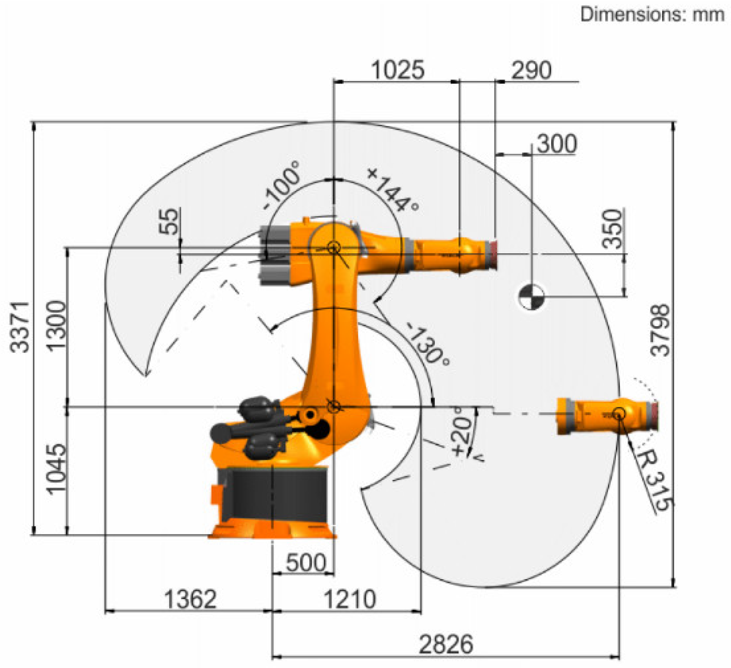
The simulation model was established based on the rigid body length parameters of the typical 6R robot KUKA KR500 and then the simulation model was used to verify the dynamic model.

First, the simulation model is established with ADAMS software; second, the required linkages and drivers are set, and the dynamic simulation is performed; third, the required parameters of the simulation process are measured; finally, the dynamic parameter identification model and the dynamic model are verified based on the measured parameters.

The structure parameters of the KR500 robot are shown in Figure 8.

The length of each rigid body $B_i (i=1,2,\cdots ,6)$ is known. To simplify the dynamic model, each $B_i$ is regarded as a homogeneous cylinder and the radius of each $B_i$ is given, among them, the rigid body $B_6$ is the end effector and its size parameters are set to 0.3 m in length and 0.3 m in radius.

Then the material type of all rigid bodies $B_i$ is set to steel and the mass $m_i (i=1,2,\cdots ,6)$ and the principal moment of inertias $J_{i_{11}}^{(i)},J_{i_{22}}^{(i)},J_{i_{33}}^{(i)} (i=1,2,\cdots ,6)$ of each rigid body are generated, then the ADAMS simulation model of the KR500 robot is established, as shown in Figure 9. The establishment and direction of each body-fixed base $(O_i,{\underset{¯}{\mathit{e}}}^{(i)}) \left(i=1,2,\cdots ,n\right)$ of the model is shown in Figure 2.

To quantify each parameter, set the unit of each physical quantity. The unit of each physical quantity is shown in

Table 1. The unit of each physical quantity.

Physical Quantity	Length	Mass	Force	Time	Angle	Frequency
Unit	m	kg	N	s	1 (rad)	Hz

. The value of gravitational acceleration is set to 9.80665 and the direction is the $-{\mathit{e}}_3^{(0)}$ direction.

The parameters of each rigid body in the ADAMS simulation model obtained from the units of each physical quantity are shown in

Table 2. Physical parameters of each rigid body $B_i$.

$\mathbf{Rigid} \mathbf{Body} {\mathit{B}}_{\mathit{i}}$	${\mathit{B}}_1$	${\mathit{B}}_2$	${\mathit{B}}_3$	${\mathit{B}}_4$	${\mathit{B}}_5$	${\mathit{B}}_6$
Length ($\mathrm{m}$)	1.045	1.245	1.21	0.315	0.29	0.3
Radius ($\mathrm{m}$)	0.5	0.3	0.2	0.2	0.2	0.3
$m_1$($\mathrm{kg}$)	6402.6012	2746.0726	1186.1661	308.7953	284.2877	661.7042
$J_{i_{11}}^{(i)}$($\mathrm{kg}·{\mathrm{m}}^2$)	800.3251	123.5733	23.7233	6.1759	5.6858	29.7767
$J_{i_{22}}^{(i)}$($\mathrm{kg}·{\mathrm{m}}^2$)	982.8126	416.4934	156.5838	5.6413	4.8353	19.8511
$J_{i_{33}}^{(i)}$($\mathrm{kg}·{\mathrm{m}}^2$)	982.8126	416.4934	156.5838	5.6413	4.8353	19.8511

. The rigid body sequence is from inside to outside. The principal moment of inertia $J_{i_{11}}^{(i)},J_{i_{22}}^{(i)},J_{i_{33}}^{(i)}$ is the expression of each rigid body $B_i$ in its own body-fixed base $(O_i,{\underset{¯}{\mathit{e}}}^{(i)})$. $m_i$ and $J_{i_{11}}^{(i)},J_{i_{22}}^{(i)},J_{i_{33}}^{(i)}$ retain 4 decimal places.

3.1. Simulation Verification of Dynamic Parameter Identification Model

According to the rigid body dynamics model, Equation (49), in order to identify the mass $m_i$ and the principal moment of inertia $J_{i_{11}}^{(i)},J_{i_{22}}^{(i)},J_{i_{33}}^{(i)}$ of a single rigid body $B_i$, the following parameters of the rigid body must be known.

1.

The three components of the Cardano angles of $(O_i,{\underset{¯}{\mathit{e}}}^{(i)})$ relative to $(O_0,{\underset{¯}{\mathit{e}}}^{(0)})$,

2.

The three components of ${\mathit{F}}_i$ in $(O_0,{\underset{¯}{\mathit{e}}}^{(0)})$,

3.

The three components of ${\mathit{M}}_i^{}$ in $(O_0,{\underset{¯}{\mathit{e}}}^{(0)})$,

4.

The three components of the acceleration of rigid body’s center of mass in $(O_0,{\underset{¯}{\mathit{e}}}^{(0)})$,

5.

The three components of the angular velocity of rigid body in $(O_0,{\underset{¯}{\mathit{e}}}^{(0)})$,

6.

The three components of the angular acceleration of rigid body in $(O_0,{\underset{¯}{\mathit{e}}}^{(0)})$.

To simultaneously identify the dynamic parameters of all rigid bodies with one simulation (only one movement), that is, the parameters collected in this movement can be used to identify each single rigid body, it is necessary for each rigid body to generate the above parameters at the same time in this movement to ensure that the data corresponding to each discrete time is real-time for each rigid body. This is the premise that the measured parameters can be used to identify the dynamic parameters of each rigid body at the same time.

To achieve the above purpose, the simulation is set to make the rigid body $B_1$ move along the ${\mathit{e}}_1^{(0)}$ direction (that is, the guide rail direction) with an acceleration of $2\mathrm{m}/{\mathrm{s}}^2$, while the joint $O_1$ and the joint $O_2$ rotate around the joint axis at the angular acceleration of $9.5493\mathrm{r}\mathrm{a}\mathrm{d}/{\mathrm{s}}^2$ (that is, $30°/{\mathrm{s}}^2$), all other joints are locked so that they do not rotate around the joint axis.

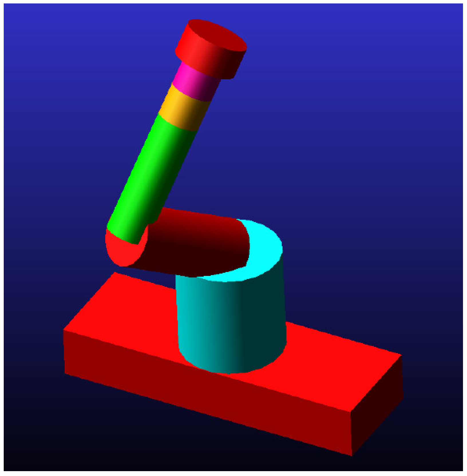
Set the initial state to the static state, and the posture is shown in Figure 9, which is the posture shown in Figure 2. The simulation termination time is 2 s and the number of steps is 100. When the simulation is terminated, the robot posture is shown in Figure 10. The motion process generates various required parameters, and the ADAMS software is used to measure various parameters.

The 6R robot system will inevitably be disturbed during the movement, which will cause errors between the measured data and the true value. To reduce the identification accuracy error caused by data error when a single set of data is used for identification, multiple sets of data can be used to identify dynamic parameters according to the mathematical model of Equation (56) to improve the accuracy and stability of the obtained parameters. Theoretically, the more data is taken, the better the identification effects, but too much data will increase the complexity and time-consuming of calculation. In this experiment, five sets of parameters are selected, respectively, taking the parameters at the five times of 0.3 s, 0.6 s, 0.9 s, 1.2 s and 1.5 s (other arbitrary times can also be randomly selected).

The dynamic parameters of the 6R robot system are identified, as shown in

Table 3. Identified 6R robot system dynamic parameters.

$\mathbf{Rigid} \mathbf{Body} {\mathit{B}}_{\mathit{i}}$	${\mathit{B}}_1$	${\mathit{B}}_2$	${\mathit{B}}_3$	${\mathit{B}}_4$	${\mathit{B}}_5$	${\mathit{B}}_6$
$m_i$($e_1^{(0)}$)($\mathrm{kg}$)	6402.6000	2746.0720	1186.1658	308.7958	284.2875	661.7041
$m_i$($e_2^{(0)}$)($\mathrm{kg}$)	—	2746.0723	1186.1661	308.7955	284.2875	661.7043
$m_i$($e_3^{(0)}$)($\mathrm{kg}$)	6402.5942	2746.0723	1186.1660	308.7955	284.2877	661.7042
$J_{i_{11}}^{(i)}$($\mathrm{kg}\cdot {\mathrm{m}}^2$)	800.3252	123.6157	23.7206	6.1761	5.6856	29.7769
$J_{i_{22}}^{(i)}$($\mathrm{kg}\cdot {\mathrm{m}}^2$)	982.8120	416.4683	156.5821	5.6412	4.8348	19.8511
$J_{i_{33}}^{(i)}$($\mathrm{kg}\cdot {\mathrm{m}}^2$)	982.8120	416.5109	156.5722	5.4619	4.8353	19.8514

.

Among them, $m_i$(${\mathit{e}}_1^{(0)}$),$m_i$(${\mathit{e}}_2^{(0)}$),$m_i$(${\mathit{e}}_3^{(0)}$) are the mass parameters of a rigid body $B_1$ identified in the ${\mathit{e}}_1^{(0)}$,${\mathit{e}}_2^{(0)}$,${\mathit{e}}_3^{(0)}$ directions, respectively. Since rigid body $B_1$ does not have acceleration in the ${\mathit{e}}_2^{(0)}$ direction, the mass cannot be identified in this direction.

The absolute error between the dynamic parameters obtained by identifying rigid body $B_6,B_5,\cdots ,B_1$ from outside to inside and its true value is shown in

Table 4. The absolute error between the dynamic parameters of rigid body $B_6,B_5,\cdots ,B_1$ and its real value.

Rigid Body	Absolute Error
	${\mathit{m}}_{\mathit{i}}$$\left({\mathit{e}}_1^{(0)}\right)$ $\left(\mathbf{kg}\right)$	${\mathit{m}}_{\mathit{i}}$$\left({\mathit{e}}_2^{(0)}\right)$ $\left(\mathbf{kg}\right)$	${\mathit{m}}_{\mathit{i}}$$\left({\mathit{e}}_3^{(0)}\right)$ $\left(\mathbf{kg}\right)$	${\mathit{J}}_{{\mathit{i}}_{11}}^{(\mathit{i})}$ $(\mathbf{kg}\cdot {\mathbf{m}}^2)$	${\mathit{J}}_{{\mathit{i}}_{22}}^{(\mathit{i})}$ $(\mathbf{kg}\cdot {\mathbf{m}}^2)$	${\mathit{J}}_{{\mathit{i}}_{33}}^{(\mathit{i})}$ $(\mathbf{kg}\cdot {\mathbf{m}}^2)$
$B_6$	−0.0001	0.0001	0	0.0002	0	0.0003
$B_5$	−0.0002	−0.0002	0	−0.0002	−0.0005	0
$B_4$	0.0005	0.0002	0.0002	0.0002	−0.0001	0.0006
$B_3$	−0.0002	0	−0.0001	−0.0027	−0.0017	−0.0116
$B_2$	−0.0006	−0.0003	−0.0003	0.0424	−0.0251	0.0175
$B_1$	−0.0012	—	−0.0070	0.0001	−0.0006	−0.0006

.

There are two reasons for the error: 1. The dynamics identification model is a complex system. To obtain the final result, many calculations are required. The result of each calculation will cause absolute errors due to only taking part of the significant digits. Therefore, the greater the number of calculations, the bigger the absolute error accumulated. 2. Since the data measured by ADAMS software retains seven significant digits and the counting rules cannot be changed, the larger the measured number, the more digits of the integer and the fewer digits of the decimals, then the greater the absolute error produced.

It can be seen from Table 4 that the absolute error of the identified mass $m_{ i}$ is very small. This is because the number of calculations for the identified mass is less. The absolute error of $m_1$ is larger than that of other $m_i (i=2,3,\cdots ,6)$. This is because the force and moment of rigid body $B_1$ is larger than that of other $B_i (i=2,3,\cdots ,6)$. The reduction in the number of decimal places of relevant data increases the absolute error.

The absolute error of the principal moment of inertia $J_{i_{11}}^{(i)},J_{i_{22}}^{(i)},J_{i_{33}}^{(i)}$ of rigid body $B_6,B_5,\cdots ,B_2$ is larger than that of mass $m_i$. This is because the principal moment of inertia $J_{i_{11}}^{(i)},J_{i_{22}}^{(i)},J_{i_{33}}^{(i)}$ is identified in the rigid body joint base $(O_i,{\underset{¯}{\mathit{e}}}^{(i)})$. The calculation process involves the coordinate transformation of parameters such as angular velocity ${\mathit{\omega }}_i$ and angular acceleration ${\dot{\mathit{\omega }}}_i$, and more calculation times cause the accumulation of absolute errors. The absolute error of the principal moment of inertia $J_{1_{11}}^{(1)},J_{1_{22}}^{(1)},J_{1_{33}}^{(1)}$ of $B_1$ is smaller than that of $J_{i_{11}}^{(i)},J_{i_{22}}^{(i)},J_{i_{33}}^{(i)} (i=2,3,\cdots ,6)$. This is because although the force and moment of $B_1$ are larger than those of other $B_i (i=2,3,\cdots ,6)$, the simplification of the identification model of $B_1$ (only the equation in the $e_1^{(1)}$ direction is retained) reduces the number of calculations.

In addition, the dynamic equation with parameter identification form is obtained by deforming the unconstrained dynamic equation, which is essentially the same equation, so the unconstrained dynamic equation is verified at the same time.

3.2. A simulation Example of the Dynamic Equation of the Constrained 6R Robot System

There are 66 equations in the constraint dynamic equation of the robot system, which can solve up to 66 unknowns, usually corresponding to 36 generalized coordinates and 30 Lagrange multipliers. Since the generalized coordinates were measured in the simulation motion, 30 Lagrange multipliers can be solved as unknowns.

Lagrange multipliers ${\lambda }_i\left(i=1,2,\cdots ,30\right)$ are written as a Lagrange multiplier matrix ${\underset{¯}{\lambda }}_i\left(i=1,2,\cdots ,6\right)$, which corresponds to rigid body $B_i\left(i=1,2,\cdots ,6\right)$. Each multiplier matrix is a five-order column matrix. For ease of description, it is recorded as:

$${\underset{¯}{\lambda }}_i=\left[\begin{array}{ccccc}{\lambda }_{i1}& {\lambda }_{i2}& {\lambda }_{i3}& {\lambda }_{i4}& {\lambda }_{i5}\end{array}\right].$$

(112)

${\lambda }_{ij}\left(j=1,2,\cdots ,5\right)$ denotes the five elements of B and each element has its physical meaning. Among them, ${\lambda }_{i1},{\lambda }_{i2},{\lambda }_{i3}$ is proportional to the ideal constraint force of the rigid body in the ${\mathit{e}}_1^{(0)},{\mathit{e}}_2^{(0)},{\mathit{e}}_3^{(0)}$ direction and corresponds one to one. ${\lambda }_{i4},{\lambda }_{i5}$ is the function of the three Cardan angles ${\alpha }_i,{\beta }_i,{\gamma }_i$ of $B_i$, which is proportional to the ideal constraint moment represented by the Cardano angle ${\alpha }_i,{\beta }_i,{\gamma }_i$.

The data at 1.5 s time is taken, and the Lagrange multipliers are calculated.

The result is calculated by Formula (111) as follows (the result retains seven significant digits):

$${\underset{¯}{\lambda }}_6={\left[\begin{array}{ccccccccc}1.356146\times {10}^{-4}& ⋮& 3.870958\times {10}^{-4}& ⋮& -6.489101\times {10}^3& ⋮& 1.211238\times {10}^3& ⋮& 8.093237\times {10}^2\end{array}\right]}^{\mathrm{T}}.$$

(113)

$${\underset{¯}{\lambda }}_5={\left[\begin{array}{ccccccccc}5.154353\times {10}^{-4}& ⋮& -2.726663\times {10}^{-4}& ⋮& -9.277012\times {10}^3& ⋮& -1.631801\times {10}^{10}& ⋮& -2.442163\times {10}^{10}\end{array}\right]}^{\mathrm{T}}.$$

(114)

$${\underset{¯}{\lambda }}_4={\left[\begin{array}{ccccccccc}-3.836233\times {10}^{-4}& ⋮& 30.072190\times {10}^{-4}& ⋮& -1.230526\times {10}^4& ⋮& 8.285916\times {10}^3& ⋮& 5.536472\times {10}^3\end{array}\right]}^{\mathrm{T}}.$$

(115)

$${\underset{¯}{\lambda }}_3={\left[\begin{array}{ccccccccc}2.941508\times {10}^{-4}& ⋮& 3.263078\times {10}^{-4}& ⋮& 2.393758\times {10}^4& ⋮& -1.431100\times {10}^{11}& ⋮& -2.141792\times {10}^{11}\end{array}\right]}^{\mathrm{T}}.$$

(116)

$${\underset{¯}{\lambda }}_2={\left[\begin{array}{ccccccccc}1.797760\times {10}^{-3}& ⋮& 1.664961\times {10}^{-4}& ⋮& -5.086735\times {10}^4& ⋮& -1.233380\times {10}^{11}& ⋮& -1.845883\times {10}^{11}\end{array}\right]}^{\mathrm{T}}.$$

(117)

$${\underset{¯}{\lambda }}_1={\left[\begin{array}{ccccccccc}4.197760\times {10}^{-3}& ⋮& 1.664961\times {10}^{-4}& ⋮& -1.136554\times {10}^5& ⋮& -5.868432\times {10}^3& ⋮& -1.877410\times {10}^{-4}\end{array}\right]}^{\mathrm{T}}.$$

(118)

Qualitative analysis of the data of ${\underset{¯}{\lambda }}_i\left(i=1,2,\cdots ,6\right)$ at 1.5 s time shows that:

To counteract the effect of gravity, the ideal constraint force of the rigid body $B_i\left(i=1,2,\cdots ,6\right)$ in the ${\mathit{e}}_3^{(0)}$ direction in this pose is much greater than in the ${\mathit{e}}_1^{(0)},{\mathit{e}}_2^{(0)}$ directions, so ${\lambda }_{i3}\left(i=1,2,\cdots ,6\right)$ is much greater than ${\lambda }_{i1},{\lambda }_{i2}\left(i=1,2,\cdots ,6\right)$. The rigid body $B_i\left(i=1,2,\cdots ,6\right)$ needs to bear all the gravity of $B_j\left(j>i\right)$ and the ideal constraint force of the rigid body in the ${\mathit{e}}_3^{(0)}$ direction from the outside to the inside increases, so ${\lambda }_{i3}\left(i=1,2,\cdots ,6\right)$ increases with decreasing $i$ number. The ideal constraint force of $B_i\left(i=1,2,\cdots ,6\right)$ in the ${\mathit{e}}_1^{(0)},{\mathit{e}}_2^{(0)}$ direction does not bear gravity; therefore, its values are all small and basically the same order of magnitude.

The shaft axes of the inside joints $O_2,O_3,O_5$ of the rigid bodies $B_2,B_3,B_5$ are in the ${\mathit{e}}_2^{(i)}$ direction and need to bear the moment generated by the gravity of the outside body, so the ideal constraint moment $O_2,O_3,O_5$ bear is large. The shaft axes of the inside joints $O_1,O_2,O_6$ of $B_1,B_4,B_6$ are not in the direction ${\mathit{e}}_2^{(i)}$ and do not need to bear the moment generated by the gravity of the outside body, so the ideal restraining moment of $O_1,O_2,O_6$ is small. Therefore, the value of ${\lambda }_{i4},{\lambda }_{i5}\left(i=2,3,5\right)$ is much greater than ${\lambda }_{i4},{\lambda }_{i5}\left(i=1,4,6\right)$.

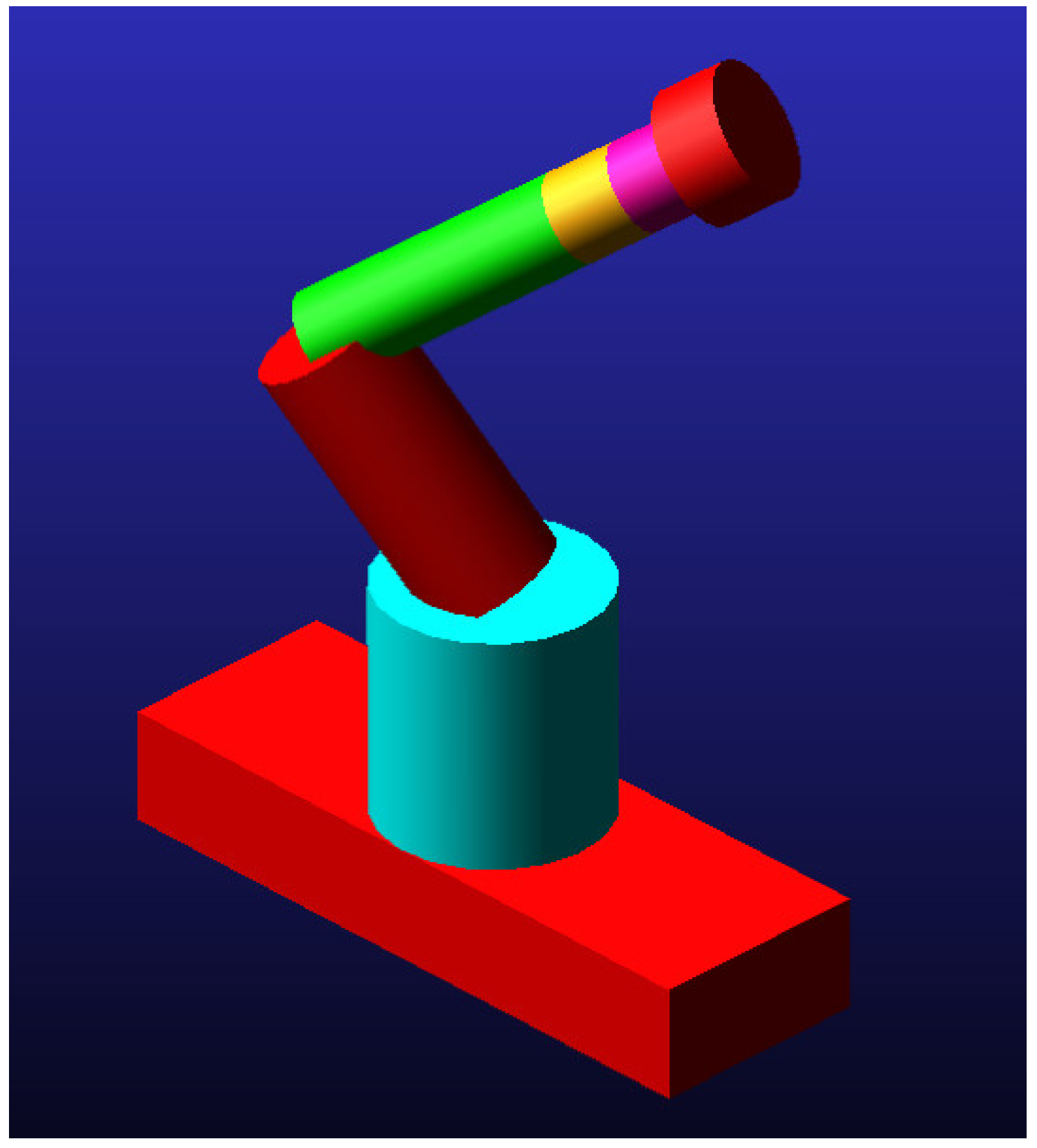
$O_2,O_3$ has more outside bodies than $O_5$ and the moment generated by the gravity of the outside bodies is larger, so ${\lambda }_{i4},{\lambda }_{i5}\left(i=2,3\right)$ is greater than ${\lambda }_{i4},{\lambda }_{i5}\left(i=5\right)$, the posture of the robot system at 1.5 s is shown in Figure 11. At this moment, the direction of the moment generated by the gravity of $B_2$ received by $O_2$ is opposite to the moment generated by the gravity of $B_i\left(i=3,4,5,6\right)$ received by $O_2$, which cancels part of the moment that $B_i\left(i=3,4,5,6\right)$ enacts on $O_2$. Therefore, the ideal constraint moment of $O_2$ is less than $O_3$, so ${\lambda }_{i4},{\lambda }_{i5}\left(i=2\right)$ is less than ${\lambda }_{i4},{\lambda }_{i5}\left(i=3\right)$.

This qualitative analysis evaluates ideal constraint force and moment. It not only intuitively describes the force situation of the ideal constraint force and moment of each joint, but also accurately describes the magnitude relationship of each the ideal constraint force and moment by the value of the Lagrange multiplier. This provides a theoretical basis for the analysis of the structural strength and reliability of 6R robot systems.

4. Conclusions

6R robot dynamics research is of great significance to the application of robots in the manufacturing industry. Motivated by this, this article systematically studied the 6R robot dynamic model in three respects: modeling, experiment and solution.

First, we established the unconstrained dynamics equation of 6-DOF industrial robots based on graph theory. On this basis, we proposed a new method of dynamic parameter identification. The results of the ADAMS simulation experiment showed that the identified dynamic parameters have extremely high accuracy, with a maximum absolute error of 0.0424, verifying the correctness and accuracy of the dynamic equation.

Second, we established the system of constraint equations for the robot system, consisting of 30 constraint equations.

Finally, we used the Lagrange multiplier method to establish the constrained dynamics equation of the 6-DOF industrial robot and pointed out that the Lagrange multiplier was proportional to the ideal constraint force and moment.

By calculating the constraint dynamics equation at the time of 1.5 s, the values of the Lagrange multipliers were calculated, and from this, the ideal constraint force and moment of the 6R robot system was qualitatively analyzed. A method to evaluate the ideal constraint force and moment was proposed.

The results of experimental research and numerical calculation show that the modeling theory and method proposed in this paper are correct and effective, and the dynamic model has high accuracy.

In future work, we will realize force control and drive control based on the constrained dynamic equation of 6-DOF industrial robots.

References

- Pham, A.-D.; Ahn, H.-J. High Precision Reducers for Industrial Robots Driving 4th Industrial Revolution: State of Arts, Analysis, Design, Performance Evaluation and Perspective. Int. J. Precis. Eng. Manuf.-Green Technol. 2018, 5, 519–533. [Google Scholar] [CrossRef]
- Menon, M.; Asada, H. Design and Control of Paired Mobile Robots Working Across a Thin Plate with Application to Aircraft Manufacturing. IEEE Trans. Autom. Sci. Eng. 2011, 8, 614–624. [Google Scholar] [CrossRef]
- Verl, A.; Valente, A.; Melkote, S.; Brecher, C.; Ozturk, E.; Tunc, L.T. Robots in machining. CIRP Ann.-Manuf. Technol. 2019, 68, 799–822. [Google Scholar] [CrossRef]
- Kim, S.H.; Nam, E.; Ha, T.I.; Hwang, S.-H.; Lee, J.H.; Park, S.-H.; Min, B.-K. Robotic Machining: A Review of Recent Progress. Int. J. Precis. Eng. Manuf. 2019, 20, 1629–1642. [Google Scholar] [CrossRef]
- Kheddar, A.; Caron, S.; Gergondet, P.; Comport, A.; Tanguy, A.; Ott, C.; Henze, B.; Mesesan, G.; Englsberger, J.; Roa, M.A.; et al. Humanoid Robots in Aircraft Manufacturing: The Airbus Use Cases. IEEE Robot. Autom. Mag. 2019, 26, 30–45. [Google Scholar] [CrossRef] [Green Version]
- Summers, M. Robot Capability Test and Development of Industrial Robot Positioning System for the Aerospace Industry. SAE Trans. 2005, 114, 1108–1118. [Google Scholar] [CrossRef]
- Yun, Y.; Li, Y. Design and analysis of a novel 6-DOF redundant actuated parallel robot with compliant hinges for high precision positioning. Nonlinear Dyn. 2010, 61, 829–845. [Google Scholar] [CrossRef]
- Shirinzadeh, B.; Teoh, P.L.; Tian, Y.; Dalvand, M.M.; Zhong, Y.; Liaw, H.C. Laser interferometry-based guidance methodology for high precision positioning of mechanisms and robots. Robot. Comput. Manuf. 2010, 26, 74–82. [Google Scholar] [CrossRef]
- Nubiola, A.; Bonev, I.A. Absolute calibration of an ABB IRB 1600 robot using a laser tracker. Robot. Comput. Integr. Manuf. 2013, 29, 236–245. [Google Scholar] [CrossRef]
- Pan, Z.; Zhang, H.; Zhu, Z.; Wang, J. Chatter analysis of robotic machining process. J. Mater. Process. Technol. 2006, 173, 301–309. [Google Scholar] [CrossRef]
- Swevers, J.; Verdonck, W.; De Schutter, J. Dynamic Model Identification for Industrial Robots. IEEE Control Syst. Mag. 2007, 27, 58–71. [Google Scholar] [CrossRef]
- Guo, Y.; Dong, H.; Wang, G.; Ke, Y. Vibration analysis and suppression in robotic boring process. Int. J. Mach. Tools Manuf. 2016, 101, 102–110. [Google Scholar] [CrossRef]
- Zhang, L.; Wang, J.; Chen, J.; Chen, K.; Lin, B.; Xu, F. Dynamic modeling for a 6-DOF robot manipulator based on a centrosymmetric static friction model and whale genetic optimization algorithm. Adv. Eng. Softw. 2019, 135, 102684. [Google Scholar] [CrossRef]
- Koopaee, M.J.; Pretty, C.; Classens, K.; Chen, X. Dynamical Modeling and Control of Modular Snake Robots with Series Elastic Actuators for Pedal Wave Locomotion on Uneven Terrain. J. Mech. Des. 2020, 142, 1–46. [Google Scholar] [CrossRef]
- Cui, M.-Y.; Xie, X.-J.; Wu, Z.-J. Dynamics Modeling and Tracking Control of Robot Manipulators in Random Vibration Environment. IEEE Trans. Autom. Control. 2012, 58, 1540–1545. [Google Scholar] [CrossRef]
- Liu, S.; Wu, L.; Lu, Z. Impact dynamics and control of a flexible dual-arm space robot capturing an object. Appl. Math. Comput. 2007, 185, 1149–1159. [Google Scholar] [CrossRef]
- Xu, W.; Meng, D.; Chen, Y.; Qian, H.; Xu, Y. Dynamics modeling and analysis of a flexible-base space robot for capturing large flexible spacecraft. Multibody Syst. Dyn. 2014, 32, 357–401. [Google Scholar] [CrossRef]
- Wu, H.; Wang, Y.; Li, M.; Alsaedi, M.; Handroos, H. Chatter suppression methods of a robot machine for ITER vacuum vessel assembly and maintenance. Fusion Eng. Des. 2014, 89, 2357–2362. [Google Scholar] [CrossRef]
- Armstrong, B.; Khatib, O.; Burdick, J. The explicit dynamic model and inertial parameters of the PUMA 560 arm. In Proceedings of the IEEE International Conference on Robotics and Automation, San Francisco, CA, USA, 7–10 April 1986; pp. 510–518. [Google Scholar]
- Zhou, Y.; Luo, J.; Wang, M. Dynamic coupling analysis of multi-arm space robot. Acta Astronaut. 2019, 160, 583–593. [Google Scholar] [CrossRef]
- Khalil, W.; Dombre, E. Modeling, Identification and Control of Robots; Hermes Penton Ltd.: London, UK, 2002. [Google Scholar]
- Wu, J.; Wang, J.; You, Z. An overview of dynamic parameter identification of robots. Robot. Comput.-Integr. Manuf. 2010, 26, 414–419. [Google Scholar] [CrossRef]
- Liu, W.; Huo, X.; Liu, J.; Wang, L. Parameter identification for a quadrotor helicopter using multivariable extremum seeking algorithm. Int. J. Control Autom. Syst. 2018, 16, 1951–1961. [Google Scholar] [CrossRef]
- Urrea, C.; Saa, D. Design and Implementation of a Graphic Simulator for Calculating the Inverse Kinematics of a Redundant Planar Manipulator Robot. Appl. Sci. 2020, 10, 6770. [Google Scholar] [CrossRef]
- Urrea, C.; Pascal, J. Parameter identification methods for real redundant manipulators. J. Appl. Res. Technol. 2017, 15, 320–331. [Google Scholar] [CrossRef]
- Garcia, R.R.; Bittencourt, A.C.; Villani, E. Relevant factors for the energy consumption of industrial robots. J. Braz. Soc. Mech. Sci. Eng. 2018, 40, 1–15. [Google Scholar] [CrossRef]
- Gaz, C.; Cognetti, M.; Oliva, A.; Giordano, P.R.; De Luca, A. Dynamic Identification of the Franka Emika Panda Robot with Retrieval of Feasible Parameters Using Penalty-Based Optimization. IEEE Robot. Autom. Lett. 2019, 4, 4147–4154. [Google Scholar] [CrossRef] [Green Version]
- Urrea, C.; Pascal, J. Dynamic Parameter Identification Based on Lagrangian Formulation and Servomotor-type Actuators for Industrial Robots. Int. J. Control. Autom. Syst. 2021, 19, 2902–2909. [Google Scholar] [CrossRef]
- Olsen, M.M.; Swevers, J.; Verdonck, W. Maximum Likelihood Identification of a Dynamic Robot Model: Implementation Issues. Int. J. Robot. Res. 2002, 21, 89–96. [Google Scholar] [CrossRef]
- Gautier, M.; Janot, A.; Vandanjon, P.-O. A New Closed-Loop Output Error Method for Parameter Identification of Robot Dynamics. IEEE Trans. Control. Syst. Technol. 2012, 21, 428–444. [Google Scholar] [CrossRef] [Green Version]
- Featherstone, R.; Orin, D. Robot dynamics: Equations and algorithms. In Proceedings of the 2000 ICRA. Millennium Conference. IEEE International Conference on Robotics and Automation. Symposia Proceedings (Cat. No.00CH37065), San Francisco, CA, USA, 24–28 April 2002; Volume 1, pp. 826–834. [Google Scholar] [CrossRef] [Green Version]
- Williams, J.H. Fundamentals of Applied Dynamics; John Wiley and Sons Inc.: New York, NY, USA, 1996. [Google Scholar]
- Selig, J.M. Geometrical Methods in Robotics; Springer: Singapore, 1996. [Google Scholar]
- Josephs, H.; Huston, R.L. Dynamics of Mechanical Systems; CRC Press: New York, NY, USA, 2002. [Google Scholar]
- Hamilton, S.W.R. On a General Method in Dynamics; Philosophical Transactions of the Royal Society: London, UK, 1834; p. 247. [Google Scholar]
- Hamilton, W.R. Second essay on a general method in dynamics. Philos. Trans. R. Soc. Lond. 1835, 125, 95–144. [Google Scholar] [CrossRef]
- Udwadia, F.E.; Kalaba, R.E. Analytical Dynamics: A New Approach; Cambridge University Press: Cambridge, UK, 2007. [Google Scholar]
- Birkhoff, G.D. Dynamical Systems; American Mathematical Society: Providence, RI, USA, 1927; Volume 9. [Google Scholar]
- Kane, T.R. Dynamics of nonholonomic systems. J. Appl. Mech. 1961, 28, 574–578. [Google Scholar] [CrossRef]
- Khalil, W.; Guegan, S. Inverse and Direct Dynamic Modeling of Gough–Stewart Robots. IEEE Trans. Robot. 2004, 20, 754–761. [Google Scholar] [CrossRef] [Green Version]
- Shao, P.; Wang, Z.; Yang, S.; Liu, Z. Dynamic modeling of a two-DoF rotational parallel robot with changeable rotational axes. Mech. Mach. Theory 2019, 131, 318–335. [Google Scholar] [CrossRef]
- Mancisidor, A.; Zubizarreta, A.; Cabanes, I.; Bengoa, P.; Jung, J.H. Kinematical and dynamical modeling of a multipurpose upper limbs rehabilitation robot. Robot. Comput. Manuf. 2018, 49, 374–387. [Google Scholar] [CrossRef]
- Huang, P.; Hu, Z.; Zhang, F. Dynamic modelling and coordinated controller designing for the manoeuvrable tether-net space robot system. Multibody Syst. Dyn. 2016, 36, 115–141. [Google Scholar] [CrossRef]
- Nielsen, M.C.; Eidsvik, O.A.; Blanke, M.; Schjølberg, I. Constrained multi-body dynamics for modular underwater robots—Theory and experiments. Ocean Eng. 2018, 149, 358–372. [Google Scholar] [CrossRef] [Green Version]
- Xu, F.; Wang, H.; Au, K.W.S.; Chen, W.; Miao, Y. Underwater Dynamic Modeling for a Cable-Driven Soft Robot Arm. IEEE/ASME Trans. Mechatron. 2018, 23, 2726–2738. [Google Scholar] [CrossRef]
- Djuric, A.M.; ElMaraghy, W.H. Automatic separation method for generation of reconfigurable 6R robot dynamics equations. Int. J. Adv. Manuf. Technol. 2010, 46, 831–842. [Google Scholar] [CrossRef]
- Introduction of KUKA KR500 Robot System and Its Structural Parameters. Available online: https://www.kuka.com/en-cn/products/robotics-systems/industrial-robots/kr-500-fortec (accessed on 15 October 2021).
Figure 1.
6R robot system [47].
Figure 2.
Schematic diagram of the 6R robot system body-fixed bases.
Figure 3.
The system with the tree structure and the structure diagram of the system with the tree structure of the 6R robot system. (a) The system with the tree structure of the 6R robot system; (b) the structure diagram of the system with the tree structure of the 6R robot system.
Figure 4.
The body-joint vector.