
Buzz Tweet Classification Based on Text and Image Features of Tweets Using Multi-Task Learning

Graduate School of Sciences and Technology for Innovation, Tokushima University, Tokushima 770-8506, Japan
*
Author to whom correspondence should be addressed.
Appl. Sci. 2021, 11(22), 10567; https://doi.org/10.3390/app112210567
Submission received: 24 September 2021
/
Revised: 5 November 2021
/
Accepted: 8 November 2021
/
Published: 10 November 2021
(This article belongs to the Section Biomedical Engineering)
Abstract
:This study investigates social media trends and proposes a buzz tweet classification method to explore the factors causing the buzz phenomenon on Twitter. It is difficult to identify the causes of the buzz phenomenon based solely on texts posted on Twitter. It is expected that by limiting the tweets to those with attached images and using the characteristics of the images and the relationships between the text and images, a more detailed analysis than that of with text-only tweets can be conducted. Therefore, an analysis method was devised based on a multi-task neural network that uses both the features extracted from the image and text as input and the buzz class (buzz/non-buzz) and the number of “likes (favorites)” and “retweets (RTs)” as output. The predictions made using a single feature of the text and image were compared with the predictions using a combination of multiple features. The differences between buzz and non-buzz features were analyzed based on the cosine similarity between the text and the image. The buzz class was correctly identified with a correctness rate of approximately 80% for all combinations of image and text features, with the combination of BERT and VGG16 providing the highest correctness rate.
1. Introduction
With the development of social networking services (SNSs), information can be shared and spread in real time among many users. This has led to frequent trends in internet content. The phenomenon of an explosion of popularity in a short period of time is called “buzz.” Marketing that utilizes this “buzz” phenomenon is attracting attention as a kind of corporate strategy. There are many examples of successful buzz marketing, including Ezaki Glico’s “Pocky Day” event on 11 November, Softbank’s “Free Mobile Phone Bills for Life Campaign”, and Seven-Eleven’s “Beard Straws” among others. These campaigns have increased the number of people accessing their websites by utilizing the diffusion power of SNSs. For marketing purposes, it would be useful if such trends on the web, triggered by SNS content, could be quickly detected.
In addition, many of the so-called “buzzed” tweets that cause a buzz phenomenon on Twitter are posted with images. Twitter has a character limit (140 full-size characters and 280 half-size characters, as of September 2021) for posted text. Therefore, complex information that is difficult to express in short sentences can be easily conveyed by attaching images or links to other pages, which is thought to increase the likelihood of the buzz phenomenon.
In this study, a method is proposed to classify tweets with images as buzz tweets or non-buzz tweets based on the image and text features of the post. Tweets that have been buzzed (buzz tweets) and tweets that have not been buzzed (non-buzz tweets) were collected. A neural network model was constructed to predict whether a tweet is a buzz tweet or not, using the text and image features of the tweets as inputs. The proposed method was evaluated and its effectiveness in correctly classifying the tweets was confirmed.
2. Related Works
In the following subsections, previous studies on buzz tweet classification are introduced, as well as studies related to information diffusion prediction. The differences between these studies and ours are discussed.
2.1. Buzz Detection from SNSs
Matsumoto et al. [1] proposed a method of classifying tweets that were buzzed and those that were not, based on the characteristics of Twitter reply texts. It is difficult to use Matsumoto et al.’s method for actual prediction because there are not many replies in the state preceding the buzz. In their research, they did not use objective indicators such as the number of retweets (RTs) or likes to classify a post. Thus, whether a post had been buzzed or not was largely based on the subjective judgment of the collector. In this study, instead of separating buzz from non-buzz tweets based on subjective criteria, the threshold of the number of likes is set to determine buzz objectively. This method is superior to conventional methods in terms of versatility and accuracy.
There have been studies focusing on hashtag. Ma et al. [2] identified hashtags based on their distribution across topics. Tsur et al. [3] predicted hashtags by applying a regression model to the content and context of the posts. Zhang et al. [4] predicted hashtags using a nonlinear model. Anusha et al. [5] used hashtags as an indicator to estimate user interest. They used sentiment analysis to analyze the interest in hashtags and conducted trend analysis to predict trends in hashtag usage and diffusion. Related studies on buzz prediction by Jansen et al. [6] and Deusser et al. [7] attempted to detect buzz using Facebook data.
2.2. Research on Predicting Information Diffusion
Alsuwaidan et al. [8] proposed a model to predict information diffusion based on the mechanism of radiation energy transfer. This model predicts the diffusion graph of information in the entire community based on certain interests. Their proposed RADDIFF model accurately captures the information diffusion process in space and time and measures the level of impact a particular influencer has in each diffusion process. However, in predicting the graph of information diffusion, the focus is mainly on the influencer, the community to which the user belongs, and the relevance of other users, which is different from our approach, which focuses on the tweet content itself to predict buzz tweets.
Fiok et al. [9] studied the prediction of response metrics available on Twitter, such as “likes,” “replies,” and “retweets.” They used data from the official Twitter account of the U.S. Navy and developed a feature-based model derived from structured tweet-related data. In addition, they applied a deep learning feature extraction approach to analyze the text and defined a task to classify tweets into three classes: low, medium, and high response tweets, employing four machine learning classifiers. Their best model achieved an F1 score of 0.655. They concluded that additional information in images and links of the tweets can be leveraged to significantly improve the performance of the models.
In terms of research on analyzing the diffusion of information on SNSs, Hatua et al. [10] predicted the amount, sentiment, and impact of tweets by means of long short-term memory (LSTM). Zhang et al. [11] proposed a cascade model that takes into account the temporal and structural characteristics of the actual influence cascade. Benabdelkrim et al. [12] introduced an exhaustive enumeration method to extract target overlapping communities from a multi-layered local network.
2.3. Predicting the Number of “Likes” for Influencer Recommendations in SNS Advertising
Yamazaki et al. [13] conducted a study to predict the number of tweets based on past tweet data of users engaged in advertising activities on SNSs, called influencers. Their study also considered images as features. In our study, the focus is only on the text of tweets without narrowing down the data to influencers or advertising tweets to make a wide range of analysis possible.
Yoo et al. [14] found that when urgent information needs to be disseminated, internal dissemination through social media networks proceeds much faster than information from external sources. Riquelme et al. [15] and Anger et al. [16] calculated the social networking potential (SNP) of tweets by considering the ratio of retweets to mentions. Chen et al. [17] proposed a multi-view influence role clustering (MIRC) algorithm that groups Twitter users into five categories. They analyzed the diffusion of tweets and the influence of users. In addition, there have been several studies on predicting words expected to become popular in SNSs. Tanaka et al. [18] predicted word trends on Twitter. Chang et al. [19] claimed that Twitter data can be used to improve both web and tweet rankings. Bhattacharya et al. [20] used a social annotation-based methodology to first infer the topics of popular Twitter users, and then transitively infer the interests of the users who follow them. Finally, Li et al. [21] proposed a learning-to-rank method for the dynamic context of advertising to estimate the interest of users on specific topics.
3. Materials and Methods
In this section, the steps involved in our proposed method and the techniques used in each step are outlined.
3.1. Overview of the Proposed Method
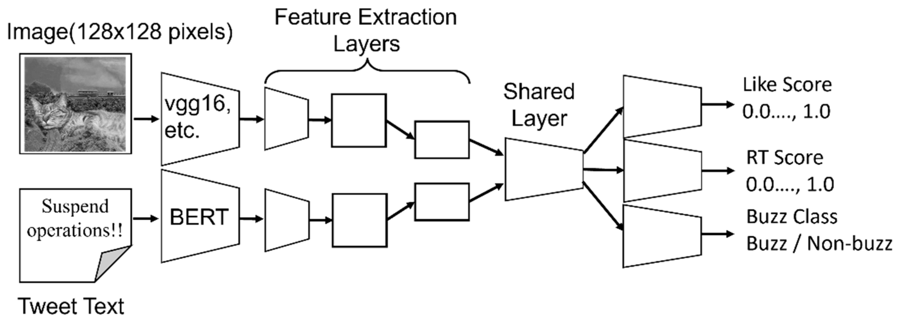
Initially, the Twitter API [22] is used to collect data on the number of likes, RTs, texts, and images of the target tweets. The text of the collected tweets is vectorized using bidirectional encoder representations from transformers (BERT) [23], and the images are vectorized using models such as VGG16 [24], ResNet50 [25], Inception V3 [26], and Xception [27]. A multi-task learning neural network model is created that uses each vector as an input to predict the number of likes, RTs, and buzz classes.
In this study, the buzz class is defined as follows: a tweet with more than 1000 likes at the time of collection is called a buzz tweet, and a tweet with less than 1000 likes is called a non-buzz tweet. The number of RTs is related to the buzz phenomenon, but it is difficult to determine the threshold because some tweets such as advertisements by official accounts of companies are retweeted very often.
3.2. Feature Extraction from Tweet Text
In this study, feature vectors are extracted from utterance text using a pre-trained model of BERT [28], which was created using a corpus of Japanese spoken language, and published by Retriever Corporation. The Japanese spoken language BERT is said to have higher expressive power than conventional BERT for utterance texts. The Japanese spoken language BERT was used because Twitter posts are likely to contain spoken words.
BERT is a large-scale model consisting of a transformer network with an encoder-decoder structure, which can be trained with a mask language model and a next-sentence prediction task to acquire a distributed representation of the language that can be applied to a variety of tasks. In BERT, distributed representations, assigned to special tokens, called CLS tokens, are often used as distributed representations of sentences in classification tasks. In this study, the distributed representation of the CLS tokens was extracted as features of the utterance text. The dimensionality of this feature was 768.
“BertJapaneseTokenizer”, a standard Japanese tokenizer for BERT was used to split the tweets into word units. As a pre-processing step, link addresses, such as images in tweets, were removed using pattern matching on regular expressions. The average 768-dimensional vector of variance representation of the CLS tokens obtained for each line was used as the BERT vector of the input tweet. For the Japanese spoken language BERT, three models (1–6_layer-wise, TAPT512_60k, DAPT) were prepared. One model (1–6_layer-wise) fine-tuned the corpus of spoken Japanese (CSJ) from layer 1 to layer 6 of BERT, pertaining to syntactic structures in Japanese. The task-adaptive pretraining TAPT512_60k model fine-tuned all layers to be task-adaptive, using CSJ. The domain-adaptive pretraining DAPT128-TAPT512 is a domain-adaptive model based on CSJ and parliamentary proceedings data. As the purpose of this study was to obtain text features of tweets, TAPT512_60k was adapted to all layers of spoken language as the pre-trained model. The distributed representation of the 768-dimensional CLS tokens was extracted from the layer immediately preceding the final layer. The vocabulary of this model consisted of 32,000 items.
3.3. Extraction of Image Features
Several pre-trained models were used for feature extraction from images. In this study, the following seven pre-trained models were trained to classify over 1,000,000 images from the ImageNet database into 1000 different object categories.
- VGG16: 512 dimensions
- ResNet50: 2048 dimensions
- Inception V3: 2048 dimensions
- Xception: 2048 dimensions
- DenseNet: 1024 dimensions
- NASNet: 4032 dimensions
- InceptionResNetV2: 1536 dimensions
To extract these image features, pre-trained models prepared in the Keras module of Tensorflow were used. The weights of the network were obtained by carrying out training on the ImageNet database. In the case of both networks, features were extracted from the layer immediately preceding the output layer. Although it is possible to fine-tune these networks, in the proposed method, image features from these seven trained networks are used to transfer learning for buzz classification. In addition, each image feature is used separately to compare and identify features that work effectively.
3.4. Multi-Task Learning of RTs, Likes, and Buzz Classes
In the proposed method, the input consists of text and image features, and a neural network is trained to predict the score of the number of RTs and the number of likes, which are further converted into four patterns of numerical values in the quartile range, and into the binary value of buzz/non-buzz (buzz class).
Both the number of RTs and the number of likes tend to increase with the size of the buzz phenomenon, but the difference between the two values depends on factors such as the number of followers and the user’s name recognition, so they are trained as separate prediction targets.
In multi-task learning, learning efficiency and prediction accuracy are expected to improve more than learning task-specific models [29]. The network for multitask learning is illustrated in Figure 1. The same loss function, mean square error (MSE), is used for both RTs and likes. The concatenation layer is used as the sharing layer. Batch normalization is applied to the input layer.
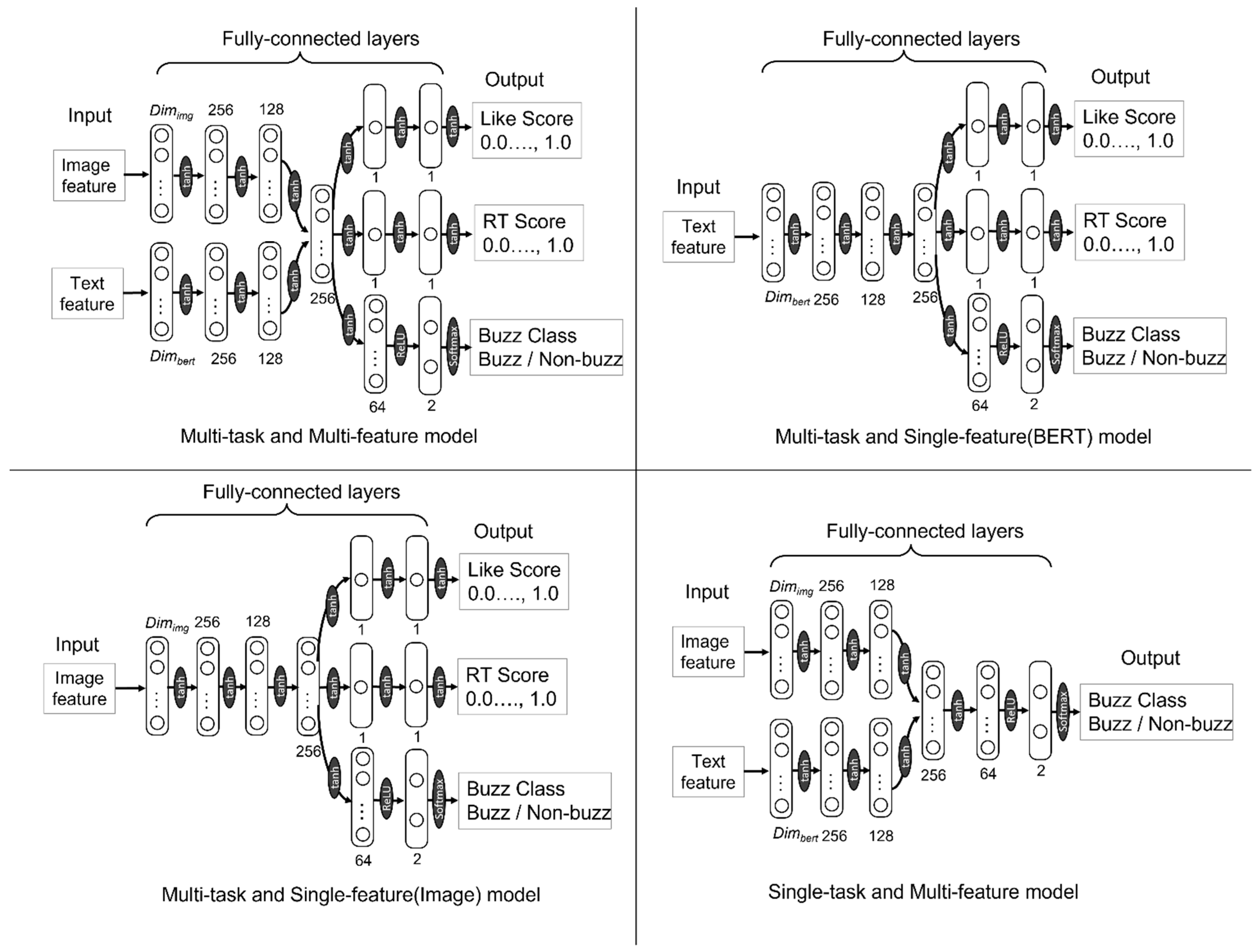
The architectures of the multitask and single-task networks are displayed in Figure 2. In both networks, a dropout function was applied to the third layer. The dropout rate was assumed to be 0.3. In the layer that outputs the buzz class, the softmax function was used as the activation function, and in the other output layers, the tanh (hyperbolic tangent function) was used. This is because normalizing the scores of the number of likes and RTs in the quartile range may cause the numbers to become negative. Activation functions other than the output layer are shown in Figure 2.
4. Experiments
4.1. Dataset
In this experiment, tweets containing keywords that represent topics associated with a large number of tweets are mainly targeted during the collection period. Examples of such keywords are listed in Table 1. The period of tweet collection was from March to June 2021, and the search condition for the Twitter API was that the tweets contained keywords and images. The actual number of tweets collected for the experiment was 508 tweets, with more than 1000 likes and an additional 9272 tweets.
Because an imbalance in the class balance of the data affects the training of the classification model, 508 non-buzz tweets with the same number of tweets were randomly selected for the experiment along with 508 tweets in the buzz class, which is the minority class.
The most common words included in the tweets were “cats” and “clouds” in the buzz tweets, and coronavirus-related tweets such as emergency declarations and vaccines in non-buzz tweets. The frequently appearing words are listed in Table 2. Buzz tweets contained few words related to coronavirus, indicating that although there were many tweets on the topic of the coronavirus, the number of likes did not increase.
The average text length of a tweet was 39 characters for buzz tweets and 93 characters for non-buzz tweets, which was more than twice as long as that of buzz tweets. The buzz tweets were easier to read because the text was shorter, and the images contained more information.
From the text of the tweets, the distributed representation vectors were extracted using spoken BERT and from the attached images. The feature vectors were extracted using any of the seven models, including VGG16. The images were used after converting the size to 128 × 128 pixels.
4.2. Training Parameters
The training parameters of the neural network are described as follows. The number of training epochs was 200; the batch size was 512; the ratio of training data to validation data was 9:1; and Adam (adaptive moment estimation) was used as the optimization algorithm. A default learning rate of 0.001 was used to determine the learning rate.
4.3. Evaluation Method
We extracted text and image features from the collected tweets, randomly divided them into training data and test data (4:1). The training and testing (five-part cross-validation) was repeated to evaluate the results. A multi-task learning neural network was constructed which accepted the feature vectors from the text and images as input to predict the number of likes, RTs, and buzz classes. From the output buzz class and the original tweet information, the correct prediction rate, the receiver operating characteristic curve (ROC), and the area under curve (AUC) were calculated and evaluated.
In addition, for comparison, a model was created with text or image features as input alone to evaluate the correct response rate. The correct response rate here refers to accuracy, which is the percentage of correctly predicted tweets from all prediction results. The formula in Equation (1) was used to calculate accuracy.
As shown in Table 3, the true positive (TP) is the number of buzz tweets correctly judged as buzz; true negative (TN) is the number of non-buzz tweets correctly judged as non-buzz; false positive (FP) is the number of non-buzz tweets incorrectly judged as buzz; and false negative (FN) is the number of buzz tweets incorrectly judged as non-buzz.
5. Results
Table 4 shows the results of the predicted correct response rate of the buzz class for each image feature model obtained in the experiment, Table 5 shows the results of prediction using only text features, and Table 6 shows the results of prediction using only image features. Table 7 shows the results of prediction using single task learning model.
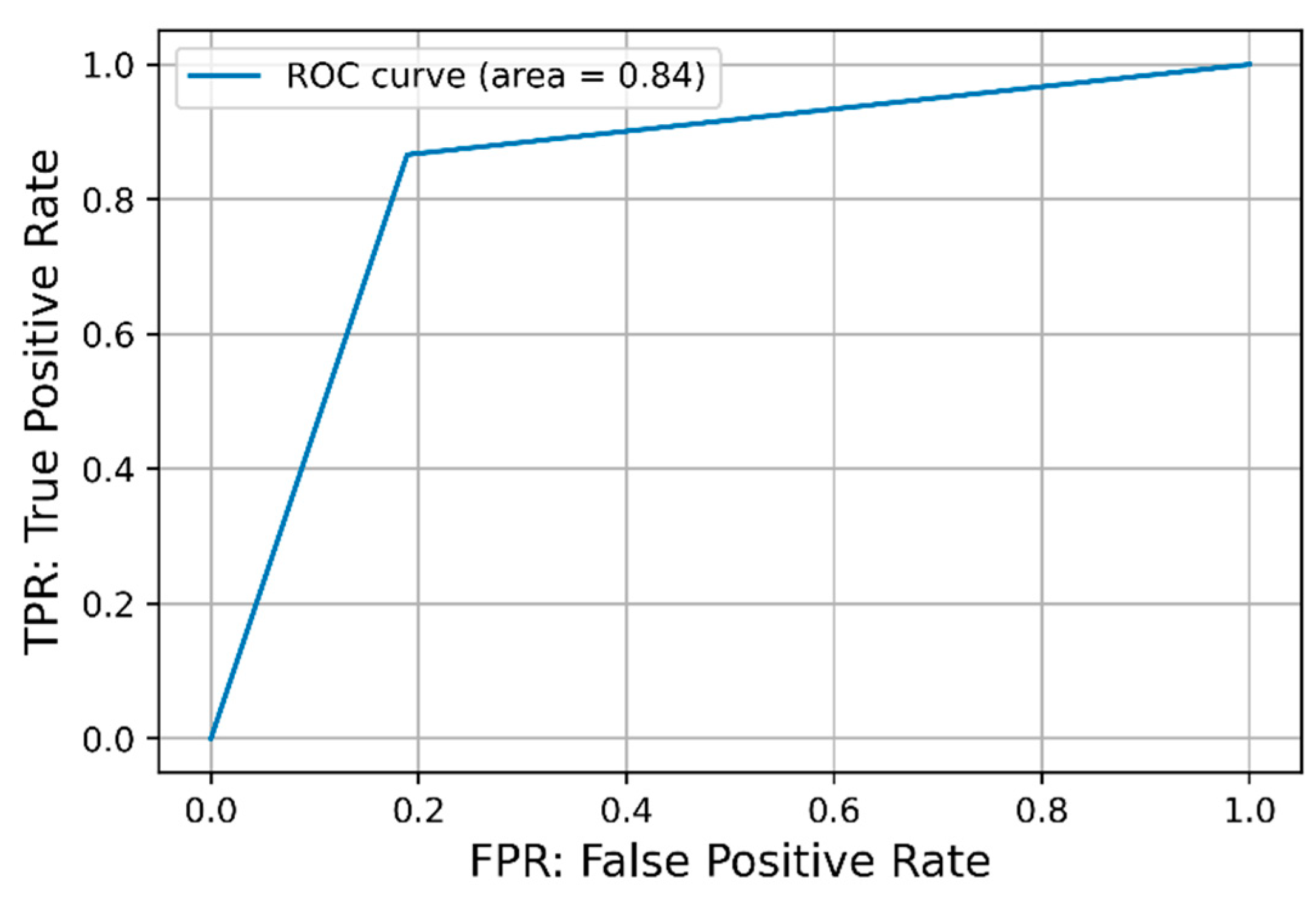
In addition, the ROC curve and the AUC calculated from the ROC curve are shown in Table 8. Figure 5 displays the ROC curve for text features and VGG16, which yielded the highest AUC.
These results show that when both text and image features are used as the input, there is little difference in the prediction accuracy rate, approximately 80%, irrespective of the type of image feature. When only text or only image features were used as input, the correct response rate of 0.82 was the highest prediction result, associated with text features alone.
In contrast, when using only image features, there was a slight difference in the correct response rate for each image feature type. The lowest correct rate was 0.49 for InceptionResnetV2 and the highest was 0.75 for VGG16.
As for the accuracy of the single-task results for predicting buzz/non-buzz, compared with the multi-task results, the accuracy decreased for all models. This confirms the effectiveness of multi-task learning. In particular, when Xception is used as an image feature, the accuracy of a single task changes significantly.
Here, the probability that the tweets were misclassified when predicted using only image features was investigated by comparing them to the set of tweets that were misclassified when predicted using a combination of text and image features. The higher the probability that the misclassified tweets are included in the set of tweets predicted by a combination of text and image features, the more the image features contribute to the prediction. Let X be the set of misclassified tweets in the prediction of the combination of text features and image features, and Y be the set of misclassified tweets in the prediction of image features alone; the agreement rate MRerror of misclassification can be expressed as in Equation (2).
It was observed that the tweets that were misclassified when only image features were used for prediction were consistent with about half of the tweets that were misclassified when text and image features were combined. It was also observed that MRerror was relatively high for image features (ResNet50, VGG16, etc.), which had relatively high correct prediction rates when only image features were used as the input.
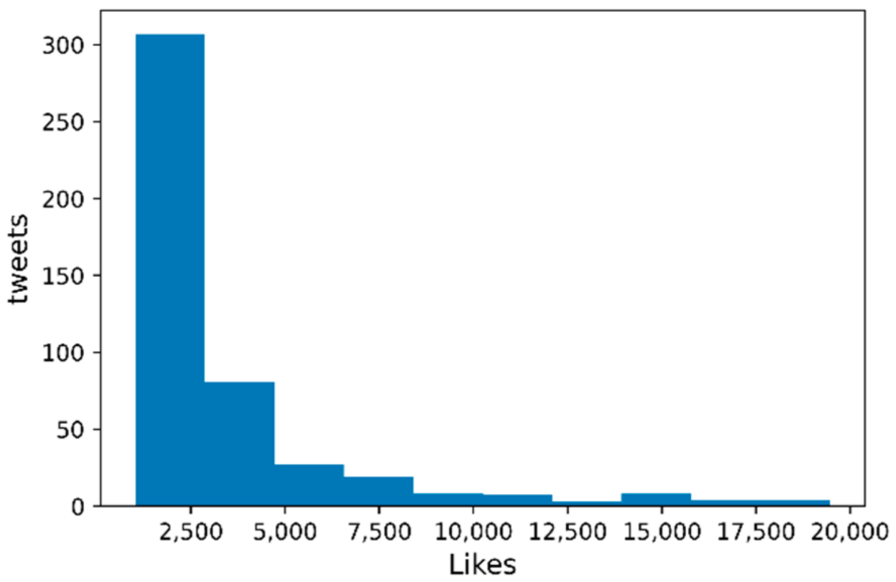
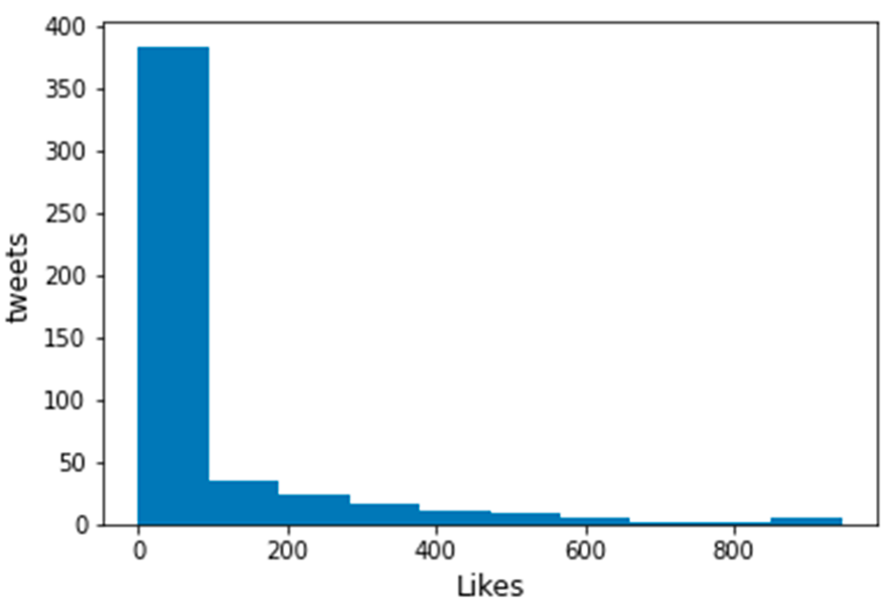
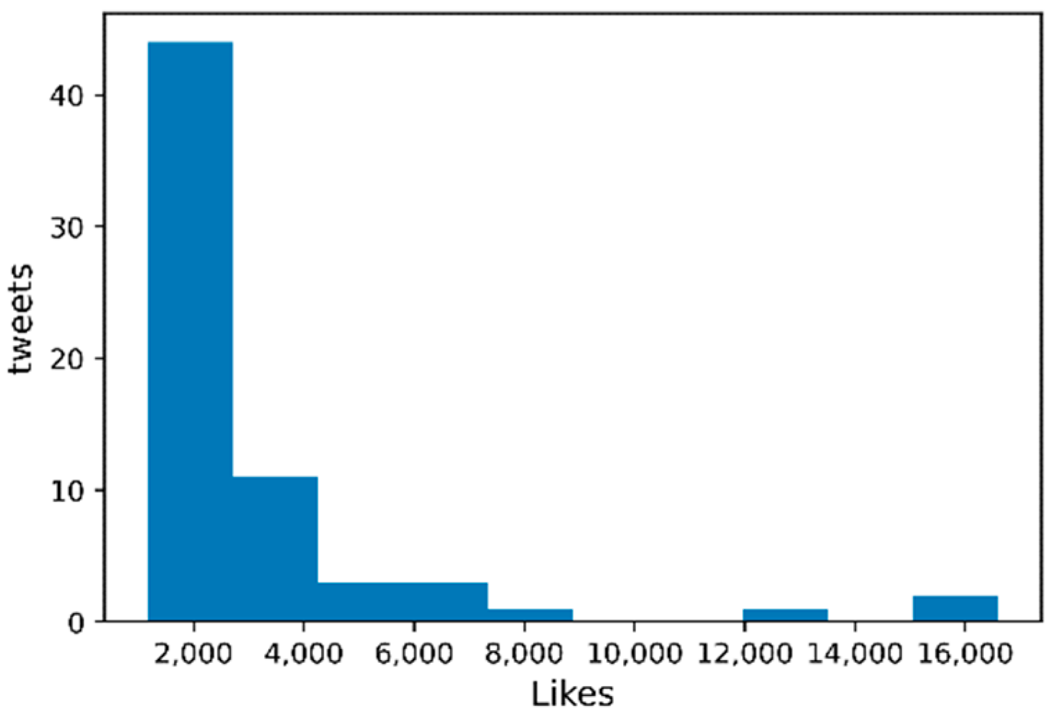
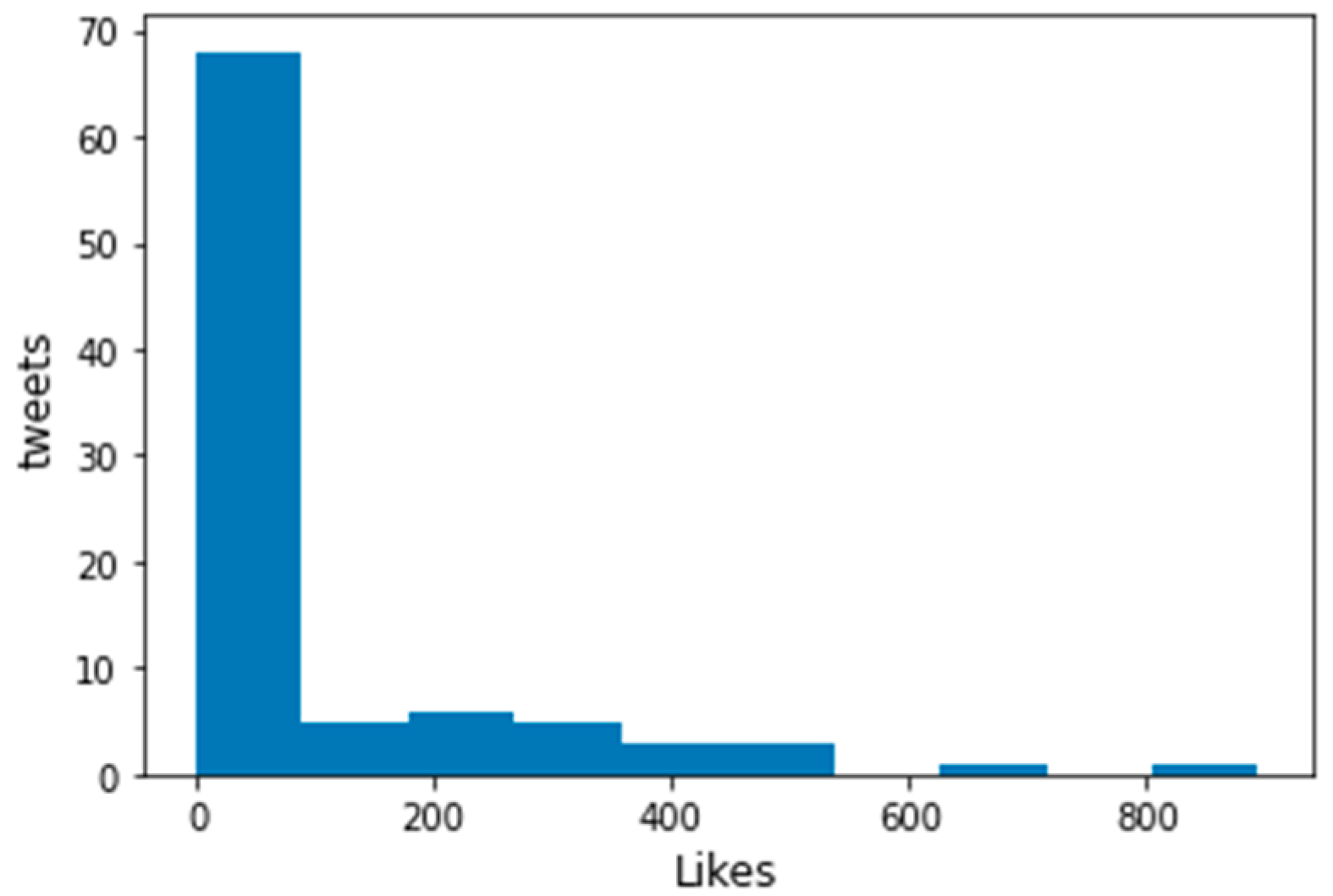
Figure 6 and Figure 7 show the distribution of the number of likes for tweets misclassified by BERT + VGG16. Figure 6 shows the misclassification of buzz tweets, and Figure 7 shows the misclassification of non-buzz tweets.
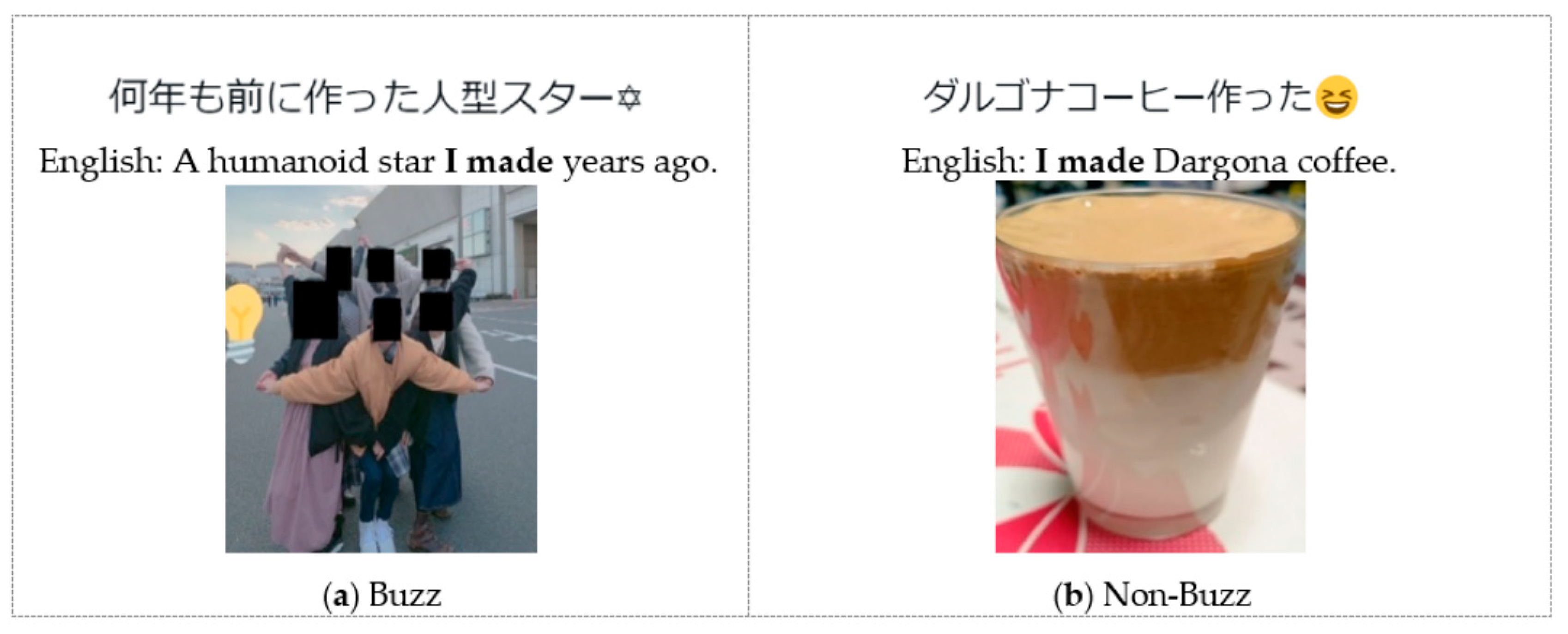
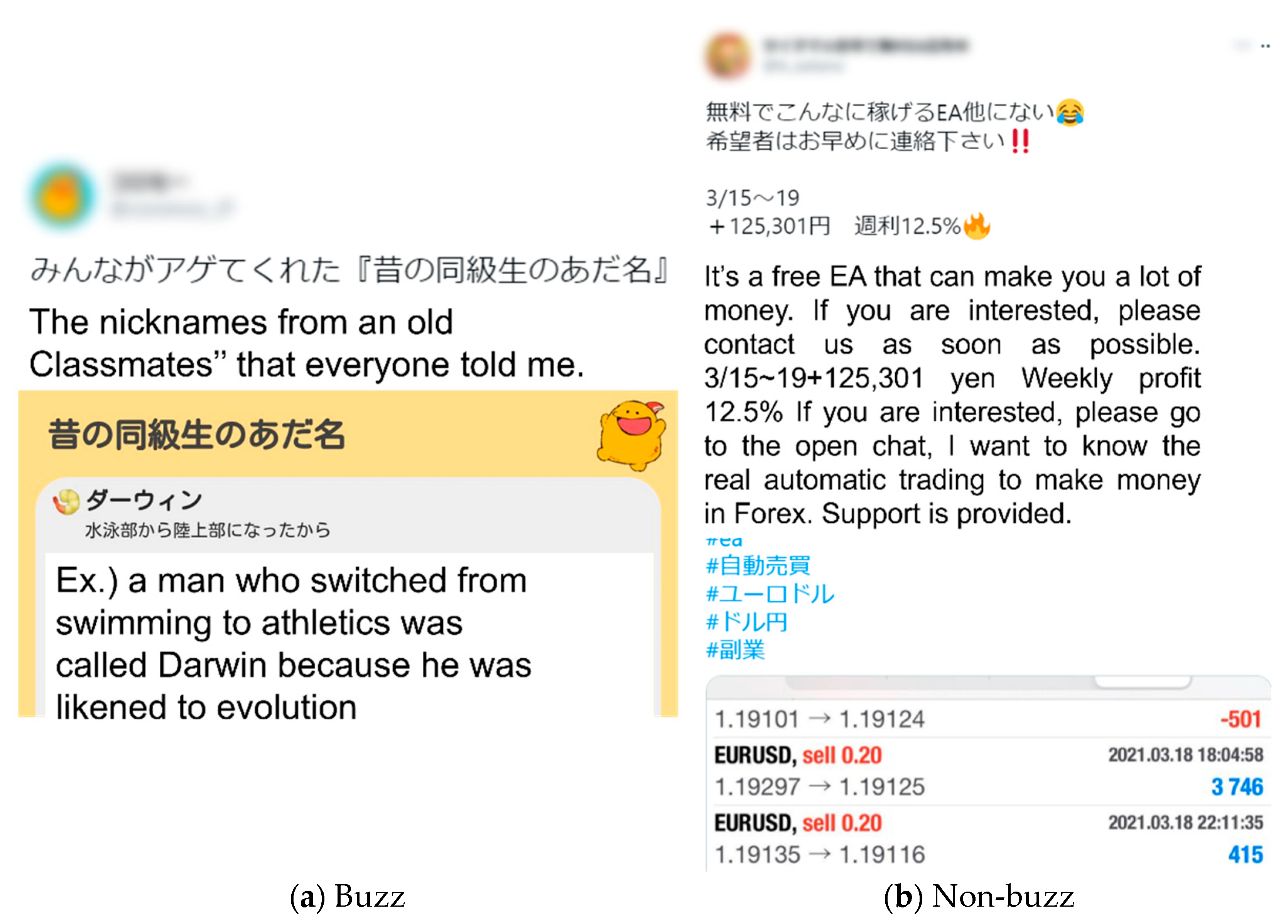
An example of text and image tweets with high similarity between text features (BERT) in buzz and non-buzz tweets is displayed in Figure 8. The cosine similarity of text features (BERT) between these tweets was 0.91, and the cosine similarity between image features (VGG16) was 0.29. The high similarity between the text features (BERT) indicates that the text meanings are similar. In contrast, the similarity between the image features was 0.29, which is not a high value, although the colors and composition of the images seemed to be similar.
Next, examples with a high similarity between images were analyzed. An example of a pair of tweets with high similarity in image features is displayed in Figure 9. In the case of these two tweets, the cosine similarity of VGG16 was 0.912, and the similarity of ResNet50 was 0.949. The cosine similarity was presumably high because the images contain text and are similar in format and color.
The cosine similarity of the two BERTs was 0.635, and there was not much similarity between the texts. The cosine similarity in DenseNet was also high, at 0.902. The non-buzz tweets were often product information tweets, and the text and images tended to be in a certain form, so the likes and RTs tended not to increase significantly.
The reason for the increase in the number of likes and RTs of buzz tweets was not the text itself or the combination of text and images, but the text contained in the images, which was considered to be interesting. These tweets tended to get more likes and RTs because they were compiled by tweeting a topic in advance, and then other users replied to the tweet with their answers, indicating that they found the tweet interesting.
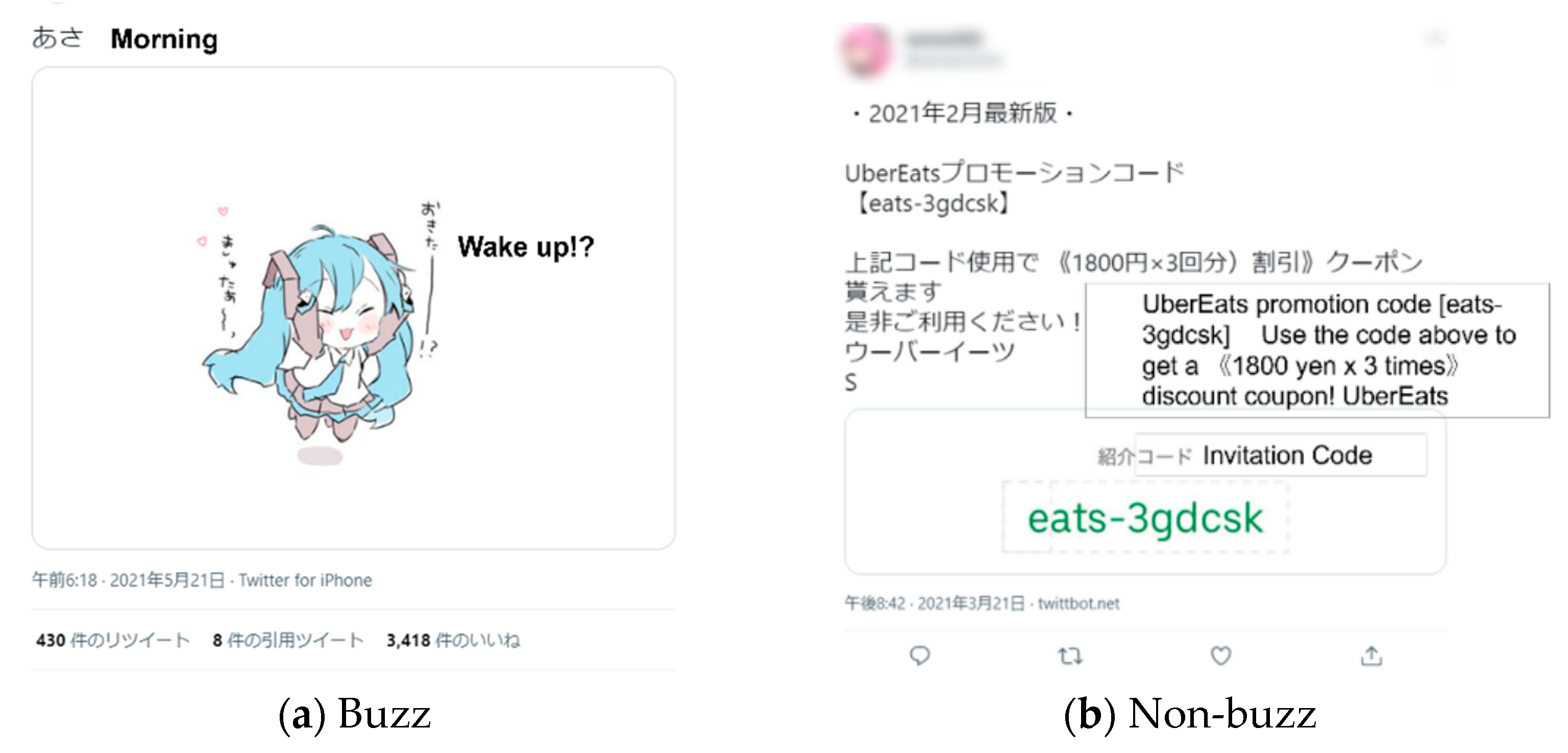
Figure 10 shows another example of a pair of tweets that have high similarity in image features. The cosine similarity of these tweets was 0.975 in DenseNet. However, it is difficult to find commonalities between these images, and the white background of the image and the position of the drawn objects may be the factors contributing to the increase in cosine similarity. The cosine similarity of BERT was about 0.678; the cosine similarity of VGG16 was about 0.637; and that of ResNet50 was about 0.872. In BERT, it is difficult to find similarities between sentences, so these values are reasonable. In VGG16, the categories of the images are judged to be different and the cosine similarity is thus lower. This suggests that there are factors other than text, such as user information and images, that divide tweets with similar text into buzz and non-buzz; tweets with similar images are likewise divided into buzz and non-buzz tweets. Either there are factors other than images, or there is a difference in the relationship between text and images, leading to these results.
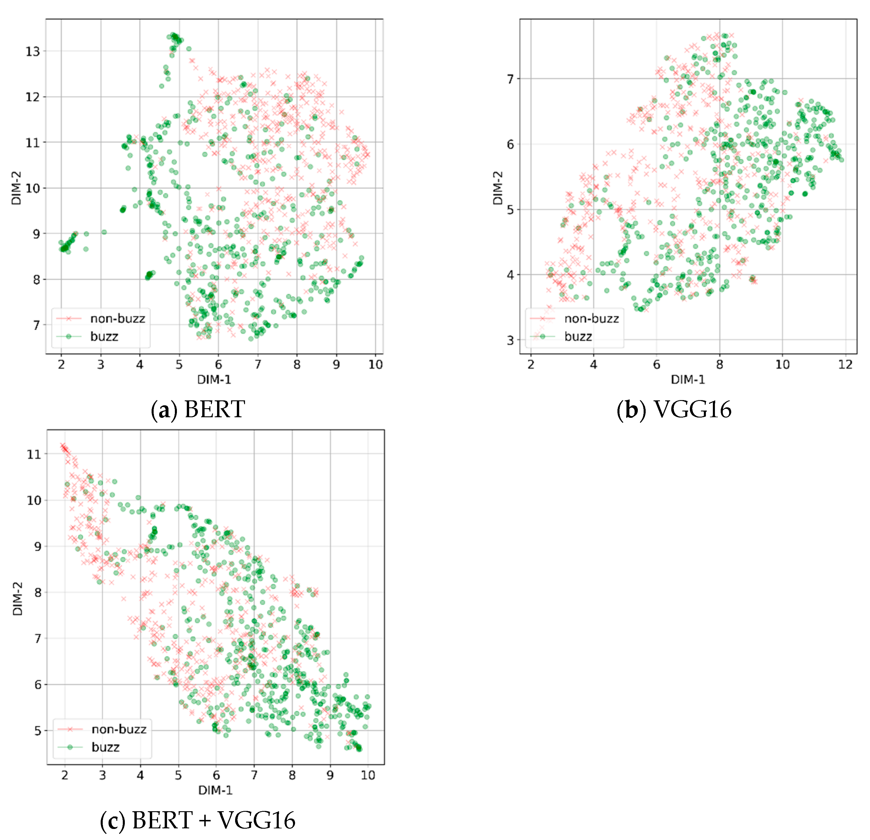
Figure 11 shows the variance representation vector of BERT, the feature vector of VGG16, and the concatenated vector of BERT and VGG16 for buzz and non-buzz tweets, dimensionally compressed using a neural autoencoder and visualized using t-SNE. In the Figure, it is not clear that there is a difference in the respective feature values. To clarify the factors of the buzz phenomenon, it is necessary to analyze the relationships among the features, rather than just looking at the distribution trend of each feature. By training a neural network, it is possible to obtain feature representations of the same number of dimensions from the intermediate layers of text and images, until they are connected. Analyzing the correlations between these feature representations provides a clue as to the cause of buzz.
6. Discussion
In the prediction of the buzz class, based on the correct prediction rate with only one of the features (text or image), it can be inferred that the text features are important. The model with the highest correct prediction rate for image features alone was VGG16 at 0.75. With both text and image features used as the input, the correct prediction rate of VGG16 for the image features was 0.84, which was higher than that of the other features.
To see if there were any similarities in the misclassification trends, the agreement rate of misclassified tweets was also examined when using either image or text features as the only input, as well as combining text and image features. As a result, the tweets with low predicted correctness using only image features exhibited a large number of misclassified tweets, but the agreement rate of misclassified tweets was approximately 0.5. This indicates that approximately half of the misclassified tweets were difficult to classify using only image features.
Although the prediction accuracy of VGG16 was higher than that of other image features, even when only image features were used, the same tweets were more likely to be misclassified when both text and image features were used, suggesting that VGG16 is a feature that is more effective when combined with BERT.
Based on the results of Figure 5 and Figure 6, it is observed that the rate at which non-buzz tweets are recognized as buzz tweets is slightly higher for the misclassified tweets. In addition, although tweets with likes close to the threshold are expected to be misclassified, this is not the case. In the case of misclassified non-buzz tweets, the misclassification is attributed to some popular words often found in buzz tweets.
With DenseNet, there were several cases in which the cosine similarity of the image features was high, such as screenshots of the same game or text in the image. With DenseNet, there were also a few images which had a high cosine similarity in the use of a white background. With VGG16, the similarity in the same category was high, and cases of no images with high similarity were attributed to the rarity of the image in the tweet. The images in Figure 5 do not seem to be similar to each other, and based on the cosine similarity results, VGG16 can discriminate the similarity of images more accurately than DenseNet and ResNet50. The correct response rate for a single image feature model also suggests that VGG16 contributes to the prediction of buzz.
The similarity between the tweets with higher BERT features may have been due to the length of the sentences and the fact that both tweets had a word in common (“made” in this example). In this example, the non-buzz tweet has a “coffee image” attached to the text “made coffee”. In contrast, the buzz tweet has a text containing the word “star” with an image of several people posing for a picture (a group photo) attached to it. This indicates that there is no direct relationship between text and images in buzz tweets, whereas a direct relationship is observed in non-buzz tweets. Thus, the difference in the relevance of text and image is considered to be the boundary between buzz and non-buzz tweets. For this reason, we believe that a model that can extract the relationship between text and images would be effective, rather than using only one or a combination of both.
7. Conclusions
In this study, a method was proposed to analyze the characteristics of tweet content as a function of tweet diffusion to classify the buzz class of tweets. Initially, the tweets were classified into buzz classes. Tweets that had an image and more than 1000 likes were considered buzz tweets, whereas tweets that had an image and less than 1000 likes were considered non-buzz tweets. In the proposed method, the text features of the tweets were extracted using the pre-trained BERT model, and the image features were obtained from pre-trained models such as VGG16. The neural network was then trained for multiple tasks. The results of the evaluation experiments showed that the correct response rate for buzz class prediction with the proposed method using both text and image features was higher than that using the features alone. However, it is not clear whether BERT or VGG16 is more suitable for buzz class prediction, so it is necessary to compare the proposed method using other options such as the simpler bag-of-words feature.
In this study, the prediction results were not evaluated for the number of likes and RTs in multi-task learning. Considering the comparison results with the buzz class prediction model using a single task, it would be effective to consider the number of likes and RTs in multi-task learning. However, the scale of the dataset used in this study is insufficient to train a model to predict the number of likes and RTs with high accuracy. In the future, we would like to construct a larger dataset to evaluate the prediction accuracy (or prediction error) of the number of likes and RTs.
The textual content of buzz and non-buzz tweets can be positive or negative, short or long. By analyzing the relationship between text and image content, a more accurate and flexible model for buzz prediction can be created. In the future, we plan to create a more accurate buzz prediction model by considering the emotional polarity of the tweet text, the sender’s profile, and other attributes as features, as well as the relevance of the attached image.
In addition, recently studied techniques such as capsule networks [30,31], aspect-oriented sentiment analysis [32,33,34,35], hybrid approaches that combine deep learning with rule-based approaches [36], and the neuro-symbolic concept learner approach [37] can be used for more accurate feature extraction and buzz analysis.
Author Contributions
Conceptualization, K.M.; Data curation, R.A.; Funding acquisition, K.M. and M.Y.; Methodology, K.M.; Supervision, K.K.; Validation, M.Y.; Visualization, K.M.; Writing—original draft, R.A.; Writing—review & editing, K.M., M.Y. and K.K. All authors have read and agreed to the published version of the manuscript.
Funding
This work was supported by the 2021 SCAT Research Grant and JSPS KAKENHI Grant Number JP20K12027, JP21K12141.
Institutional Review Board Statement
Not applicable.
Informed Consent Statement
Not applicable.
Data Availability Statement
Not applicable.
Conflicts of Interest
The authors declare no conflict of interest.
References
- Matsumoto, K.; Hada, Y.; Yoshida, M.; Kita, K. Analysis of Reply-Tweets for Buzz Tweet Detection. In Proceedings of the 33rd Pacific Asia Conference on Language, Information and Computation (PACLIC), Hakodate, Japan, 13–15 September 2019; pp. 138–146. [Google Scholar]
- Ma, Z.; Sun, A.; Cong, G. Will this #hashtag be popular tomorrow? In Proceedings of the 35th International ACM SIGIR Conference on Research and Development in Information Retrieval (SIGIR’12), New York, NY, USA, 12–16 August 2012; pp. 1173–1174. [Google Scholar] [CrossRef]
- Tsur, O.; Rappoport, A. What’s in a Hashtag? In Proceedings of the Fifth International Conference on Web Search and Web Data Mining, Seattle, WA, USA, 8–12 February 2012; pp. 643–652. [Google Scholar] [CrossRef]
- Zhang, P.; Wang, X.; Li, B. On Predicting Twitter Trend: Factors and Models. In Proceedings of the International Conference on Advances in Social Network Analysis and Mining, Niagara Falls, ON, Canada, 25–28 August 2013. [Google Scholar]
- Anusha, A.; Singh, S. Is That Twitter Hashtag Worth Reading. In Proceedings of the Third International Symposium on Women in Computing and Informatics, Kochi, India, 10–13 August 2015; pp. 272–277. [Google Scholar] [CrossRef] [Green Version]
- Jansen, N.; Hinz, O.; Deusser, C.; Strufe, T. Is the Buzz on?—A Buzz Detection System for Viral Posts in Social Media. J. Interact. Mark. 2021, 56, 1–17. [Google Scholar] [CrossRef]
- Deusser, C.; Jansen, N.; Reubold, J.; Schiller, B.; Hinz, O.; Strufe, T. Buzz in Social Media: Detection of Short-lived Viral Phenomena. In Proceedings of the Web Conference 2018, WWW’18, Lyon, France, 23–27 April 2018; pp. 1443–1449. [Google Scholar] [CrossRef]
- Alsuwaidan, L.; Ykhlef, M. Information Diffusion Predictive Model Using Radiation Transfer. IEEE Access 2017, 5, 25946–25957. [Google Scholar] [CrossRef]
- Fiok, K.; Karwowski, W.; Gutierrez, E.; Ahram, T. Predicting the Volume of Response to Tweets Posted by a Single Twitter Account. Symmetry 2020, 12, 1054. [Google Scholar] [CrossRef]
- Hatua, A.; Nguyen, T.; Sung, A. Information Diffusion on Twitter: Pattern Recognition and Prediction of Volume, Sentiment, and Influence. In Proceedings of the Fourth IEEE/ACM International Conference on Big Data Computing, Applications and Technologies, Austin, TX, USA, 5–8 December 2017; pp. 157–167. [Google Scholar] [CrossRef] [Green Version]
- Zhang, Z.; Zhao, W.; Yang, J.; Paris, C.; Nepal, S. Learning Influence Probabilities and Modelling Influence Diffusion in Twitter. In Proceedings of the 2019 World Wide Web Conference, San Francisco, CA, USA, 13–17 May 2019; pp. 1087–1094. [Google Scholar] [CrossRef]
- Benabdelkrim, M.; Savinien, J.; Robardet, C. Finding Interest Groups from Twitter Lists. In Proceedings of the 35th Annual ACM Symposium on Applied Computing, Brno, Czech Republic, 30 March–3 April 2020; pp. 1885–1887. [Google Scholar] [CrossRef] [Green Version]
- Yamazaki, K.; Ushiama, T. Predicting the Number of “Likes” for Influencer Recommendation in SNS Advertising. DEIM Forum, 1–3 March 2021. Available online: https://db-event.jpn.org/deim2021/index.html (accessed on 9 November 2021). (In Japanese).
- Yoo, E.; Rand, W.; Eftekhar, M.; Rabinovich, E. Evaluating information diffusion speed and its determinants in social media networks during humanitarian crises. J. Oper. Manag. 2016, 45, 123–133. [Google Scholar] [CrossRef]
- Riquelme, F.; González-Cantergiani, P. Measuring user influence on Twitter: A survey. Inf. Process. Manag. 2016, 52, 949–975. [Google Scholar] [CrossRef] [Green Version]
- Anger, I.; Kittl, C. Measuring Influence on Twitter. In Proceedings of the 11th International Conference on Knowledge Management and Knowledge Technologies, Graz, Austria, 7–9 September 2011; pp. 1–4. [Google Scholar] [CrossRef]
- Chen, C.; Gao, D.; Li, W.; Hou, Y.; Wong, K.-F.; Gao, W.; Xu, R. Inferring Topic-Dependent Influence Roles of Twitter Users. In Social Media Content Analysis: Natural Language Processing and Beyond; World Scientific: Singapore, 2017; Chapter 6; pp. 225–235. [Google Scholar] [CrossRef]
- Tanaka, K.; Tajima, K. Predicting word trends on Twitter. DEIM Forum 2017, D6-2. Available online: https://db-event.jpn.org/deim2017/proceedings.html (accessed on 9 November 2021). (In Japanese).
- Chang, Y.; Dong, A.; Kolari, P.; Zhang, R.; Inagaki, Y.; Diaz, F.; Zha, H.; Liu, Y. Improving Recency Ranking Using Twitter Data. ACM Trans. Intell. Syst. Technol. 2013, 4, 1–24. [Google Scholar] [CrossRef] [Green Version]
- Bhattacharya, P.; Zafar, M.; Ganguly, N.; Ghosh, S.; Gummadi, K. Inferring User Interests in the Twitter Social Network. In Proceedings of the 8th ACM Conference on Recommender Systems, Foster City, CA, USA, 6–10 October 2014; pp. 357–360. [Google Scholar] [CrossRef] [Green Version]
- Li, C.; Lu, Y.; Mei, Q.; Wang, D.; Pandey, S. Click-through Prediction for Advertising in Twitter Timeline. In Proceedings of the 21th ACM SIGKDD International Conference on Knowledge Discovery and Data Mining, Sydney, Australia, 10–13 August 2015; pp. 1959–1968. [Google Scholar] [CrossRef] [Green Version]
- Twitter API. Available online: https://developer.twitter.com/en/docs/twitter-api (accessed on 9 November 2021).
- Devlin, J.; Chang, M.-W.; Lee, K.; Toutanova, K. BERT: Pre-Training of Deep Bidirectional Transformers for language Understanding. In Proceedings of the 2019 Conference of the North American Chapter of the Association for Computational Linguistics: Human Language Technologies, Minneapolis, MN, USA, 2–7 June 2019; Volume 1, pp. 4171–4186. [Google Scholar]
- Simonyan, K.; Andrew Zisserman, A. Very Deep Convolutional Networks for Large-Scale Image Recognition. In Proceedings of the International Conference on Learning Representations (ICLR2015), San Diego, CA, USA, 7–9 May 2015; pp. 1–14. [Google Scholar]
- He, K.; Xiangyu Zhang, X.; Ren, S.; Sun, J. Deep Residual Learning for Image Recognition. In Proceedings of the 2016 IEEE Conference on Computer Vision and Pattern Recognition (CVPR), Las Vegas, NV, USA, 27–30 June 2016; Volume 1, pp. 770–778. [Google Scholar]
- Szegedy, C.; Vanhoucke, V.; Ioffe, S.; Shlens, J. Rethinking the Inception Architecture for Computer Vision. In Proceedings of the IEEE Conference on Computer Vision and Pattern Recognition (CVPR), Las Vegas, NV, USA, 27–30 June 2016; pp. 2818–2826. [Google Scholar] [CrossRef] [Green Version]
- Chollet, F. Xception Deep Learning with Depthwise separable convolutions. In Proceedings of the IEEE Conference on Computer Vision and Pattern Recognition (CVPR), Honolulu, HI, USA, 21–26 July 2017. [Google Scholar] [CrossRef] [Green Version]
- Katsumata, S.; Sakata, H. Creating a Japanese Spoken Language BERT Using CSJ. In Proceedings of the 27th Annual Meeting of the Association for Natural Language Processing, Kitakyushu, Japan, 15–19 March 2021; pp. 805–810. (In Japanese). [Google Scholar]
- Ruder, S. An overview of multi-task learning in deep neural networks. arXiv 2017, arXiv:1706.05098. [Google Scholar]
- Sabour, S.; Frosst, N.; Hinton, G.E. Dynamic Routing Between Capsules. In Proceedings of the 31st Conference on Neural Information Processing Systems (NIPS 2017), Long Beach, CA, USA, 4–9 December 2017; pp. 1–11. [Google Scholar]
- Kosiorek, A.; Sabour, S.; Teh, Y.W.; Hinton, G. Stacked Capsule Autoencoders. In Proceedings of the 33rd Conference on Neural Information Processing Systems (NeurIPS 2019), Vancouver, BC, Canada, 8–14 December 2019; pp. 15486–15496. [Google Scholar]
- Zhang, Q.; Lu, R. A Multi-Attention Network for Aspect-Level Sentiment Analysis. Futur. Internet 2019, 11, 157. [Google Scholar] [CrossRef] [Green Version]
- Zainuddin, N.; Selamat, A.; Ibrahim, R. Hybrid sentiment classification on twitter aspect-based sentiment analysis. Appl. Intell. 2017, 48, 1–15. [Google Scholar] [CrossRef]
- Liang, B.; Luo, W.; Li, X.; Gui, L.; Yang, M.; Yu, X.; Xu, R. Enhancing Aspect-Based Sentiment Analysis with Supervised Contrastive Learning. In Proceedings of the 30th ACM International Conference on Information & Knowledge Management, Online, 1–5 November 2021; pp. 3242–3247. [Google Scholar] [CrossRef]
- Zhu, J.; Wang, H.; Zhu, M.; Tsou, B.K.; Ma, M. Aspect-Based Opinion Polling from Customer Reviews. IEEE Trans. Affect. Comput. 2011, 2, 37–49. [Google Scholar] [CrossRef]
- Ayo, F.E.; Folorunso, S.O.; Abayomi-Alli, A.; Adekunle, A.O.; Awotunde, J.B. Network intrusion detection based on deep learning model optimized with rule-based hybrid feature selection. Inf. Secur. J. A Glob. Perspect. 2020, 29, 267–283. [Google Scholar] [CrossRef]
- Mao, J.; Gan, C.; Kohli, P.; Tenenbaum, J.B.; Wu, J. The Neuro-Symbolic Concept Learner: Interpreting Scenes, Words, and Sentences from Natural Supervision. In Proceedings of the 7th International Conference on Learning Representations (ICLR 2019), New Orleans, LA, USA, 6–9 May 2019. [Google Scholar]
Figure 1.
Multi-task learning to predict the number of likes/RTs and the buzz class.

Figure 2.
Neural network architectures.

Figure 3.
Buzz tweet like distribution.

Figure 4.
Non-buzz tweet like distribution.

Figure 5.
ROC for text features and VGG16 model.

Figure 6.
Buzz tweet like distribution.

Figure 7.
Non-buzz tweet like distribution.

Figure 8.
Examples of tweet pairs with high similarity in text features.

Figure 9.
Examples of tweet pairs with high similarity in image features (with VGG16).

Figure 10.
Examples of tweet pairs with high similarity in image features (with DenseNet).

Figure 11.
Visualization of BERT, VGG16 and BERT + VGG16 for each buzz/non-buzz tweet.


Table 1.
Example of keywords for tweet collection.
| Cat Lover | Dog Lover |
| COVID-19 vaccine | declaration of a state of emergency |
| Taiwan castella | Uber Eats |
| remote class | GoTo travel |
Table 2.
Words that were included in many tweets.
| Buzz | Non-Buzz |
|---|---|
| cat | emergency |
| cloud | COVID-19 |
| photo | vaccine |
Table 3.
Confusion matrix of evaluation basis.
| Buzz (True Value) | Non-Buzz (True Value) | |
|---|---|---|
| Buzz (Predicted Value) | TP (True Positive) | FP (False Positive) |
| Non-buzz (Predicted Vaue) | FN (False Negative) | TN (True Negative) |
Table 4.
Comparison of accuracies between text and image features.
| Text Feature | Image Feature | Accuracy |
|---|---|---|
| BERT | DenseNet | 0.84 |
| InceptionResNetV2 | 0.82 | |
| Inception V3 | 0.83 | |
| NASNet | 0.82 | |
| ResNet50 | 0.82 | |
| VGG16 | 0.84 | |
| Xception | 0.82 |
Table 5.
Accuracy for text features only.
| Text Feature | Accuracy |
|---|---|
| BERT | 0.82 |
Table 6.
Comparison of accuracies for image features only.
| Image Feature | Accuracy |
|---|---|
| DenseNet | 0.67 |
| InceptionResNetV2 | 0.49 |
| Inception V3 | 0.52 |
| NasNet | 0.59 |
| ResNet50 | 0.71 |
| VGG16 | 0.75 |
| Xception | 0.57 |
Table 7.
Comparison of accuracy in the single task learning.
| Text Feature | Image Feature | Accuracy |
|---|---|---|
| BERT | DenseNet | 0.84 |
| InceptionResNetV2 | 0.75 | |
| Inception V3 | 0.75 | |
| NasNet | 0.75 | |
| ResNet50 | 0.82 | |
| VGG16 | 0.83 | |
| Xception | 0.68 |
Table 8.
AUC comparison for each image feature.
| Text Feature | Image Feature | AUC |
|---|---|---|
| BERT | DenseNet | 0.84 |
| InceptionResNetV2 | 0.82 | |
| InceptionV3 | 0.83 | |
| NasNet | 0.82 | |
| ResNet50 | 0.82 | |
| VGG16 | 0.84 | |
| Xception | 0.82 |
Table 9.
MRerror for each image feature.
| Text Feature | MRerror |
|---|---|
| DenseNet | 0.54 |
| InceptionResnetV2 | 0.50 |
| InceptionV3 | 0.52 |
| NasNet | 0.50 |
| ResNet50 | 0.61 |
| VGG16 | 0.68 |
| Xception | 0.55 |
Publisher’s Note: MDPI stays neutral with regard to jurisdictional claims in published maps and institutional affiliations. |
© 2021 by the authors. Licensee MDPI, Basel, Switzerland. This article is an open access article distributed under the terms and conditions of the Creative Commons Attribution (CC BY) license (https://creativecommons.org/licenses/by/4.0/).
Share and Cite
MDPI and ACS Style
Amitani, R.; Matsumoto, K.; Yoshida, M.; Kita, K. Buzz Tweet Classification Based on Text and Image Features of Tweets Using Multi-Task Learning. Appl. Sci. 2021, 11, 10567. https://doi.org/10.3390/app112210567
AMA Style
Amitani R, Matsumoto K, Yoshida M, Kita K. Buzz Tweet Classification Based on Text and Image Features of Tweets Using Multi-Task Learning. Applied Sciences. 2021; 11(22):10567. https://doi.org/10.3390/app112210567
Chicago/Turabian StyleAmitani, Reishi, Kazuyuki Matsumoto, Minoru Yoshida, and Kenji Kita. 2021. "Buzz Tweet Classification Based on Text and Image Features of Tweets Using Multi-Task Learning" Applied Sciences 11, no. 22: 10567. https://doi.org/10.3390/app112210567
Note that from the first issue of 2016, this journal uses article numbers instead of page numbers. See further details here.