Mass, Direct Cost and Energy Life-Cycle Cost Optimization of Steel-Concrete Composite Floor Structures

Abstract

This paper presents a study showing the optimization of the mass, direct (self-manufacturing) costs, and energy life-cycle costs of composite floor structures composed of a reinforced concrete slab and steel I-beams. In a multi-parametric study, mixed-integer non-linear programming (MINLP) optimizations are carried out for different design parameters, such as different loads, spans, concrete and steel classes, welded, IPE and HEA steel profiles, and different energy consumption cases. Different objective functions of the composite structure are defined for optimization, such as mass, direct cost, and energy life-cycle cost objective functions. Moreover, three different energy consumption cases are proposed for the energy life-cycle cost objective: an energy efficient case (50 kWh/m²), an energy inefficient case (100 kWh/m²), and a high energy consumption case (200 kWh/m²). In each optimization, the objective function of the structure is subjected to the design, load, resistance, and deflection (in)equality constraints defined in accordance with Eurocode specifications. The optimal results calculated with different criteria are then compared to obtain competitive composite designs. Comparative diagrams have been developed to determine the competitive spans of composite floor structures with three different types of steel I beam: those made of welded sections and those made of IPE or HEA sections, respectively. The paper also answers the question of how different objective functions affect the amount of the calculated costs and masses of the structures. It has been established that the higher (more wasteful) the energy consumption case is, the lower the obtained masses of the composite floor structures are. In cases with higher energy consumption, the energy life-cycle costs are several times higher than the costs determined in direct cost optimization. At the end of the paper, a recommended optimal design for a composite floor system is presented that has been developed on the multi-parametric energy life-cycle cost optimization, where the energy efficient case is considered. An engineer or researcher can use the recommendations presented here to find a suitable optimal composite structure design for a desired span and uniformly imposed load.

1. Introduction

The optimization of steel–concrete composite structures can generally be conducted under several relevant criteria. The minimization of mass can be one of the simpler but still useful criteria for achieving optimal structural design, see, e.g., Poitras et al. [1]. Such an optimization criterion may specifically come to the fore when foundation conditions, transportation conditions, or earthquake conditions require the lightest possible structures. Nevertheless, most researchers have focused on the minimization of the direct cost criterion that is commonly considered in the industry, where the economic parameters of different structures must be applied to the decision variables in the objective function. Recently, contemporary literature has proposed a variety of cost objective function formulations for the optimization of composite structures. These works are presented in the references by Kassapoglou [2], Kravanja and Šilih [3], Klanšek and Kravanja [4,5], Farkas and Jarmai [6], Cheng and Chan [7], Senouci and Al-Ansari [8], Kaveh and Shakouri Mahmud Abadi [9], Luo et al. [10], Kaveh and Benham [11], Kaveh and Ahangaran [12], Žula et al. [13], and Kravanja et al. [14]. In addition, Omkar et al. [15,16] formulated a problem with multiple objectives attempting to minimize the weight and cost of the composite components to achieve a specified strength. The above references testify to the fact that the applied criteria for determining the optimal design of composite structures have been determined in most cases as the objective functions of some of the specific characteristics of potential building materials (e.g., density, grades, strengths, etc.) and feasible structural dimensions.

In some published works, e.g., [7,8], constant cost coefficients have been proposed to be set in the objective function to simplify the structural optimization problem and to facilitate its solvability. However, the assumption of the invariability of cost parameters often proves to be less appropriate, especially in cases where an actual direct cost distribution is to be considered during the process of structural optimization. Therefore, nonlinear objective functions with variable cost parameters are thus preferably used in the optimization [3,4,5,6,13,14]. Regarding the required cost information to be obtained after optimization, the level of detail required for the objective function formulation may well be adjusted to make decisions about both the structural design in the general planning phase and in the exact cost calculations of the production phase. In this context, simpler formulated cost objective functions for different composite systems can be found in references [2,7,8], while more detailed functions can be found in references [4,5,6,13,14].

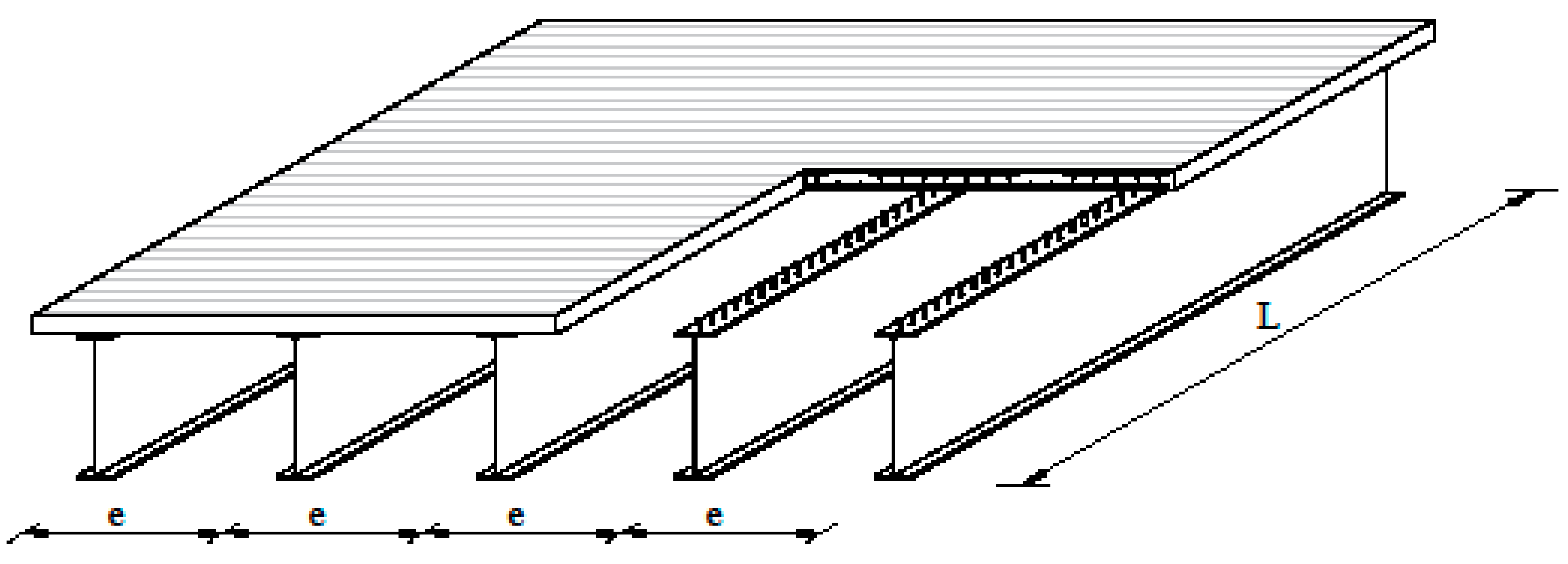
This paper presents a study demonstrating the optimization of the mass, direct (self-manufacturing) costs, and energy life-cycle costs of composite I-beam floor structures that have been composed from a reinforced concrete slab and steel I profiles with full shear connection, as seen in Figure 1. The optimizations are performed using mixed-integer non-linear programming (MINLP). MINLP is a modern optimization method that has been successfully used to solve engineering problems from a variety of fields, see, e.g., Rizki et al. [17], Chen et al. [18], Marty et al. [19], Li et al. [20], Mancò et al. [21], Kegl et al. [22], and Jelušič and Žlender [23]. It is a discrete optimization method that makes it possible to obtain real/executable structures with standard dimensions and material strengths. Since the MINLP optimizations are carried out for different parameters, such as different loads, spans, concrete- and steel classes, standard- and welded steel I profiles, and different energy consumption cases, multi-parametric MINLP optimization is applied.

In this study, the single-objective MINLP approach was used to perform the separate optimizations of the addressed structural system under the same design constraints but by considering different objectives: the minimization of mass, minimization of direct costs, and minimization of energy life-cycle costs. Thus, the optimization presented in this study is performed according to a single criterion that is most commonly used in structural optimization (see, for example, references [24,25]). Such a technique does not represent a multi-objective method, which are methods where all of the criteria are considered simultaneously in a single search process (see, e.g., references [15,16,26]). The optimization process in this paper rather falls into the domain of parametric optimization.

The multi-parametric mass optimization of composite structures was thus conducted for the above-mentioned different parameters and is presented in the paper. Since we were also interested in how energy consumption in buildings affects the cost increases and changes in the mass/material consumption of composite structures, the so-called multi-parametric energy life-cycle cost (ELCC) optimization was performed and is presented in this study as well. The performed ELCC optimizations include the costs of space heating, ventilation, and air conditioning (HVAC). In terms of ELCC analysis, see, e.g., [27], other life-cycle costs such as the costs of maintenance, inspection, repair, demolition, removal, and the transportation and deposition/recycling of the dilapidated structures are not included in the current study.

The efficiency classes derived from the standards for the energy consumption of buildings vary considerably from country to country. For this reason, a direct comparison of the energy efficiency classes and energy indicators between different countries is difficult. In most countries, buildings are considered energy efficient when energy consumption is 50 kWh/m² or below, they are deemed energy inefficient when energy consumption is around 100 kWh/m², and they are seen as highly energy inefficient when consumption is around 200 kWh/m². For more information on energy efficiency classes, see the references by Kwiatkowski and Rucińska [28] and Moore et al. [29].

As mentioned above, an annual energy consumption of less than 50 kWh per m² for space heating, ventilation, and air conditioning generally represents an energy efficient case (EEC) and good practise in the design of new houses/buildings. Although energy efficiency has increased in the last two decades due to improvements in the industrial sector and in households [30], energy consumption is still very high in existing, non-renovated buildings and is sometimes also in new buildings. For this reason, two additional cases are proposed for ELCC optimization, namely an energy inefficient case (EIC, 100 kWh/m²) and a high energy consumption case (HEC, 200 kWh/m²). Thus, when calculating the operating costs for the heating, ventilation, and air conditioning of buildings, three different energy consumption cases are considered altogether.

The optimal results calculated with the above-mentioned different criteria are then compared in order to achieve competitive composite designs. These results are also compared with the direct cost optimization results calculated and presented by Kravanja et al. [14]. Comparative diagrams are drawn. Diagrams such as the ones presented here can help researchers and engineers find a competitive composite floor structure (CFS) for a desired load and span. This study is a continuation of previous research [14], where only the multi-parametric direct cost optimization of CFSs was investigated. The added value of this paper is thus the ability to:

• Define three different objective functions of CFS to be considered when performing structural optimizations and design comparisons:

  ○

  Mass objective function;

  ○

  Direct cost objective function, as originally introduced in references Klanšek and Kravanja [4,5] and later extended in the reference written by Kravanja et al. [14];

  ○

  Energy life-cycle cost objective function, which includes direct cost items, as stated in the previous three references, and the energy operating costs required for an adequate structure use;

• Perform the multi-parametric mass optimization of CFSs;
• Perform the multi-parametric energy life-cycle cost optimization of CFSs for three different energy consumption cases:

  ○

  An energy efficient case (ELCC EEC);

  ○

  An energy inefficient case (ELCC EIC);

  ○

  A high energy consumption case (ELCC HEC);

• Develop comparative diagrams of the obtained optimal masses and energy life-cycle costs of CFSs, which can then be used to determine the competitive spans of CFSs for three different types of steel I beam sections (for the direct cost diagrams, see [14]):

  ○

  Welded I profiles;

  ○

  Standard IPE profiles;

  ○

  Standard HEA profiles;

• Investigate how different objective functions affect the costs of CFSs;
• Investigate how different objective functions affect the masses of CFSs;
• Determine recommendations for the optimal design of CFSs for an energy efficient case.

Since a number of abbreviations are used in this paper, they are listed and explained in

Table 1. List of abbreviations.

Abbreviation	Meaning
DC	direct production costs per unit of useable surface of the structure
CFS	composite floor structure (system)
CFSHEA	composite floor structure with HEA sections
CFSIPE	composite floor structure with IPE sections
CFSWIS	composite floor structure with welded I sections
EEC	energy efficient case
EIC	energy inefficient case
ELCC	energy life-cycle costs of the structure per unit of its useable surface
ELCC EEC	energy life-cycle cost criteria/optimization of an energy efficient case
ELCC EIC	energy life-cycle cost criteria/optimization of an energy inefficient case
ELCC HEC	energy life-cycle cost criteria/optimization of a high energy consumption case
GAMS	general algebraic modelling system
HEA	European wide flange section
HEC	high energy consumption case
HVAC	heating, ventilation and air conditioning
IPE	I profile European (European IPE section)
MASS	mass of the structure per unit of its useable surface
MINLP	mixed-integer non-linear programming
MILP	mixed-integer linear programming
NLP	non-linear programming
OA/ER	outer-approximation/equality-relaxation algorithm

.

2. MINLP Optimization Models

The problem of steel–concrete CFSs is a non-linear, continuous, and discrete optimization problem that can be solved by mixed-integer non-linear programming, i.e., MINLP. The general MINLP problem is formulated in the following way:

$$\min z=f(\mathbf{x},\mathbf{y})$$

subjected to:

$$\begin{gathered} \hspace{1em}\mathbf{g}(\mathbf{x},\mathbf{y})\le \mathbf{0}\hspace{1em}\left(\mathrm{MINLP}\right) \\ \mathbf{x}\in \mathrm{X}=\{\mathbf{x}\in R^n:{\mathbf{x}}^{\mathrm{LO}}\le \mathbf{x}\le {\mathbf{x}}^{\mathrm{UP}}\} \\ \mathbf{y}\in \mathrm{Y}={\{0,\mathrm{l}\}}^{\mathrm{m}} \end{gathered}$$

where x and y are the vectors of the continuous and discrete binary (0–1) variables, respectively. f(x,y) is the objective function subjected to the (in)equality constraints g(x,y) ≤ 0. Functions f(x,y) and g(x,y) must be continuous and differentiable; at least one of them must be non-linear.

For the optimization of a composite I beam floor system, see Figure 2, where a number of various optimization models were modelled according to the above MINLP formulation. These models, which were already presented by Kravanja et al. [14], are now extended to three different criteria—three different objective functions that are necessary for structures, i.e., minimization of mass, direct costs, and energy life-cycle costs. The defined objective functions are subjected to design, loading, and dimensioning constraints. The latter are determined according to Eurocode [31,32,33,34,35] specifications by taking into account the (in)equality conditions for the ultimate limit state constraints (internal forces, resistances) and the serviceability limit state constraints (deflections).

In a previous study [14], which discussed the plastic and elastic resistances of composite structures and three various positions of the neutral axes (in the web of the steel I beam, in the upper steel flange and in the concrete), it was found that the CFSs calculated with plastic resistance are 15% cheaper than those with elastic resistance when HEA and IPE profiles for steel beams are used and that they are 20% cheaper when welded I-beams are used. It was found that the composite constructions with the plastic resistance and the neutral axis in the plate are the most favourable constructions. For this reason, only the plastic resistance of the composite structures and the neutral axis located in the concrete slab are considered in this study, as seen in Figure 3.

Note that the optimization models are modelled in the GAMS (general algebraic modelling system) by Brooke et al. [36]. Most of the input data (scalars), variables, and equality and inequality constraints of the models have already been presented and shown by Žula et al. [13] and Kravanja et al. [14].

3. Different Objective Functions

In order to gain new information and comparisons about the optimal designs of composite structures, three different criteria of composite structures have been defined.

3.1. Mass Objective Function

The first criterion that is defined is the mass objective function, Equation (1). It is formulated as follows:

Minimize MASS = {ρ_c·V_c + ρ_s·(V_s + V_r)}/(e · L)

(1)

where MASS denotes the mass of the structure per unit of its useable surface, ρ_c and V_c represent the concrete density and its associated volume, ρ_s is the steel density, while V_s and V_r stand for the required volumes of structural- and reinforcing steel, respectively. The notations e and L represent the intermediate distance between the steel I sections and the longitudinal span of the composite system. Although the above mass objective function is simple, it represents a nonlinear element of the optimization model. However, the second criterion is much more complex, namely the minimization of direct (self-manufacturing) costs. Here, direct costs are determined as the sum of material costs, power consumption costs, and labour costs that are necessary for the production of the structural system.

3.2. Direct Cost Objective Function

The second criterion is the direct cost objective function, Equation (2), which is established for the treated structure in the following form:

Minimize DC = C_MAT + C_POW + C_LAB
= {C_MAT = (C_M,s + C_M,c + C_M,r + C_M,sc + C_M,e + C_M,ac,fp,tc + C_M,f + C_M,c,ng + C_M,c,oxy)/(e · L)} +
{C_POW = (C_P,c,gm + C_P,w + C_P,sw + C_P,v)/(e · L)} +
{C_LAB = (C_L,g + C_L,c,oxy-ng + C_L,p,a,t + C_L,w + C_L,sw + C_L,spp + C_L,f + C_L,r + C_L,c + C_L,v + C_L,cc)/(e · L)}

(2)

where the objective variable DC represents the direct production costs per unit of useable surface of the structure. The direct costs are defined as the sum of material costs (C_MAT), power consumption costs (C_POW), and labour costs (C_LAB) required to produce the structural system.

Material costs (C_MAT) include cost items such as structural steel (C_M,s), concrete (C_M,c), reinforcement (C_M,r), headed shear studs (C_M,sc), electrode consumption (C_M,e), anti-corrosion, fire protection and top coat painting (C_M,ac,fp,tc), floor-slab panels (C_M,f), natural gas consumption (C_M,c,ng), and oxygen consumption (C_M,c,oxy).

Power consumption costs (C_POW) include edge grinding (C_P,c,gm), shielded metal arc welding (C_P,w), stud arc welding (C_P,sw), and concrete consolidation (C_P,v).

Labour costs (C_LAB) contain edge grinding (C_L,g), steel-sheet cutting (C_L,c,oxy-ng), preparation, assembly and tacking (C_L,p,a,t), shielded metal arc welding (C_L,w), stud arc welding (C_L,sw), surface protection and preparation (C_L,spp), formwork treatment (C_L,f), reinforcing steel treatment (C_L,r), concreting the slab (C_L,c), concrete consolidation (C_L,v), and curing the concrete (C_L,cc).

For more information on the direct cost items and fabrication times (T_i), see Klanšek and Kravanja [4,5] and Kravanja et al. [14].

3.3. Energy Life-Cycle Cost Objective Function

The third criterion is the objective function of the energy life-cycle costs, Equation (3), which is given here in the following form:

Minimize ELCC = DC + ∑_i Co_i·(1 + r)^‒year_i/(e · L)

(3)

where ELCC represents the energy life-cycle costs of the composite system per unit of its useable surface, DC are the direct costs (Equation (2)), Co_i denotes the structure operating costs, and r stands for the discount rate of money where year_i indicates the years in which the corresponding costs are incurred, and the index i = 1, 2, …, n is the year counter. It should be noted that year₁ = 0 is adopted for the initial year, while the following years are defined as year₂ = 1, year₃ = 2 and so on. The structure operating costs Co_i are defined by Equation (4):

Co_i = C_HVAC · p_i · H · e · L

(4)

where C_HVAC represents the current (i.e., at the initial year, year₁ = 0) yearly cost of heating, ventilation and air conditioning (HVAC) per m³ of the air space of the structure volume, while H denotes the height of the structure. The parameter p_i is determined in order to take into account the anticipated influence of the electricity market sale price evolution on the structure’s operating costs during its design working life. The variable C_HVAC is calculated by Equation (5):

C_HVAC = ECC · EP/(CH + h + d)

(5)

where ECC is the energy consumption class parameter in kWh/m² (energy efficient case EEC, energy inefficient case EIC, and high energy consumption case HEC), EP is the electricity cost parameter in EUR /kWh, CH is the clear ceiling height (3.0 m), h is the height of the steel I beam, and d is the depth of the concrete slab.

In this study, the design working life of the structure is set to 50 years (i.e., i = 1, 2, …, 50), which is in accordance with the recommendations of Eurocode 0 [31]. As far as the life-cycle cost optimization of structures is concerned, Sarma and Adeli [37] suggest setting the discount rate of money at 2 to 3% above inflation. Here, the mentioned parameter is determined with the frequently considered value r = 0.04 (i.e., 4% discount rate). In terms of the anticipated influence of the price evolution in the electricity market sale, the parameter p_i is in the optimization model set on the basis of the data presented by Iniesta and Barroso [38] and uses the following polynomial approximation function in Equation (6):

p_i = 1 + 0.0187·year_i + 0.0012·year_i²

(6)

4. Multi-Parametric MINLP Optimization

The investigation of the optimal design of CFSs involves the multi-parametric MINLP optimization of a combination of different design parameters and superstructure alternatives, such as:

• Five alternative loads (2–10 kN/m², 2 kN/m² step);
• Ten alternative spans (5–50 m, 5 m step);
• Three alternative steel classes (S 235, S 275, S 355);
• Seven alternative concrete classes (C20/25 - C50/60);
• One hundred and twenty-three different cross-section alternatives of steel I-beams that have:

  ○

  Eighty-one welded I section alternatives, including nine alternative flange thicknesses (from 8 to 40 mm) and nine alternative web thicknesses (from 8 to 40 mm);

  ○

  Eighteen alternative IPE sections (IPE 80 - IPE 600);

  ○

  Twenty-four alternative HEA sections (HEA 100 - HEA 1000);

• Twenty-five alternative wire meshes for concrete reinforcement (R188 - 5×R524);
• Twenty-seven alternative slab depths in whole centimeters (4–30 cm);
• Two alternative centre of gravity axis positions for all-steel section:

  ○

  In the concrete plate;

  ○

  In the steel profile;

• Five different objective alternatives:

  ○

  Mass objective function (MASS);

  ○

  Direct cost objective function (DC);

  ○

  Three energy life-cycle cost objective functions of three different energy consumption cases (ELCC):

  ▪

  An energy efficient case (ELCC EEC, 50 kWh/m²);

  ▪

  An energy inefficient case (ELCC EIC, 100 kWh/m²);

  ▪

  A high energy consumption case (ELCC HEC, 200 kWh/m²).

Note that the discrete alternatives of the loads, spans, dimensions (profiles), material classes, and the positions of the centroid axis in this paper are the same as how they are they defined in reference [14], which allows a comparison between the results of the different objective functions that are used. In this way, the combinatorics of the multi-parametric study yields 1.743 × 10⁸ different structure alternatives. The defined optimization problem thus arises to the multi-parametric MINLP mass, direct cost, energy life-cycle cost, material, standard dimension, and rounded dimension optimization problem. The optimizations are performed using a MINLP program MIPSYN [39,40]. The modified outer-approximation/equality-relaxation (OA/ER) algorithm by Kravanja and Grossmann [41], the successor of the OA/ER algorithm [42], is applied. The OA/ER algorithm solves an alternative sequence of non-linear programming (NLP) and mixed-integer linear programming (MILP) problems, as seen in Figure 4. The NLP performs continuous optimization with fixed binary variables (discrete alternatives) and represents an upper bound on the minimized MINLP objective function. The MILP calculates new binary variables (discrete alternatives) that involve a global linear approximation to the superstructure of discrete alternatives and predicts a lower bound on the minimized objective function. The NLPs and MILPs must be solved sequentially. Convergence is achieved when the MILP lower bound matches the NLP upper bound. The optimization of the non-convex problem is stopped if NLPs show no improvement.

To solve the NLPs, we use GAMS/CONOPT (generalized reduced-gradient method) by Drudd [43], and to compute the MILP problems, we use GAMS/CPLEX (branch and bound method) [44]. To speed up the convergence of the modified OA/ER algorithm, a two-phase MINLP strategy [45,46] is used. The two-phase strategy starts with the continuous NLP computation at the relaxed binary variables (discrete alternatives). The computed solution including the continuous variables provides a good starting point for the next discrete optimization. In the second phase, the binary variables (discrete alternatives) are recovered, and discrete MINLP optimization (the alternative sequence of NLPs and MILPs) is guided to the optimal result.

The unit prices for manufacturing considered in the parametric optimization study are the same as those defined in reference [14]. The labour cost and steel price in high-income economies (20 EUR/h for labour and 1.25 EUR/kg for steel) are used in this study as they represent the average unit cost and price between middle-income and top-income economies and because most composite structures are constructed in this region, see the World Bank [47] and reference [14].

Typical MINLP Optimization

This paper presents the typical MINLP optimization of a 10 m long simply supported CFS that has been subjected to self-weight and uniformly distributed variable-imposed load of 6 kN/m².

The superstructure of the considered composite floor structure with welded I sections (CFSWIS) comprises 3 different classes of steel, 7 classes of concrete, 81 alternative sizes of welded I sections, 25 alternative sizes of reinforcing meshes, 27 alternatives of plate depths, and 2 alternative positions of the centroid axis, resulting in 2.296 × 10⁶ different structural alternatives (structures) as a combination between the mentioned alternatives. Similarly, 5.103 × 10⁵ different structure alternatives are defined for the composite floor structure with standard IPE profiles (CFSIPE) and 6.804×10⁵ different alternatives for the composite floor structure with standard HEA profiles (CFSHEA). A total of 3.486 × 10⁶ different structural alternatives for all three structure types is summed up. One structural alternative is the optimal structure (for the defined objective function).

Note that 15 individual MINLP optimizations of the composite structure have to be performed for 5 different objective functions (the mass, the direct cost, and three different energy life-cycle cost functions) in the combination with 3 different types of steel I beams (welded, IPE and HEA sections).

The obtained optimal results are presented in

Table 2. The optimal results.

Objective Type	Mass kg/m2	DC EUR/m2	ELCC EUR/m2
MASS objective	169.38	80.90	-
DC objective	422.97	62.29	-
ELCC EEC objective	288.63	63.64	91.81
ELCC EIC objective	217.42	65.70	118.91
ELCC HEC objective	175.45	74.67	170.38

Legend: DC, direct costs; ELCC, energy life-cycle costs; EEC, energy efficient case; EIC, energy inefficient case; HEC, high energy consumption case.

and Figure 5. While welded I sections are in the mass optimization and in the direct cost optimization calculated to be the most suitable steel beams, all three types of energy life-cycle cost optimizations exhibit IPE profiles to be optimal steel sections. The mass calculated in the direct cost optimization is about 2.5-times higher than the optimal mass optimized in the mass optimization. It should be noted that the worse the energy consumption case (from EEC to HEC) is, the lower the amount of calculated mass is. The direct costs calculated in the energy life-cycle cost optimization (for the high energy consumption case ELCC HEC) and in the mass optimization are 20% and 30% higher, respectively, than the optimal direct costs calculated in the direct cost optimization.

5. Comparative Diagrams of Competitive Spans of Composite Floor Structures for Different Objective Functions

After the MINLP calculations were carried out, the computed results and the composite designs were analyzed and compared. First, comparative diagrams were drawn to determine the competitive spans of the CFSs with welded, IPE, and HEA profiles for different objective functions.

5.1. Optimal Masses (MASS) of the Composite Floor Structures

The optimal masses of CFSs are presented. Figure 6 shows diagrams of the achieved optimal masses (kg/m²) for the structure types CFSIPE, CFSHEA and CFSWIS. The diagrams were drawn for five alternative loads that ranged from 2 kN/m² to 10 kN/m².

We found that the long-span CFSs with standard profiles exhibited very heavy and unrealistic designs. For this reason, the CFSIPE structures that are presented here are shown only for spans up to 20 m, and the CFSHEA structures are only shown for spans up to 25 m. The CFSWIS structures are drawn for all of the considered spans up to 50 m.

The diagrams show that the CFSIPE structures are the lightest structures for spans up to 7 m, while the CFSWIS structures are the lightest structures for all spans longer than 7 m. The CFSHEA system is for spans above 17 m lighter than the CFSIPE system for all loads except 2 kN/m².

5.2. Optimal Energy Life-Cycle Costs (ELCC) of the Composite Floor Structures

The diagrams in Figure 7, Figure 8 and Figure 9 represent the optimal energy life-cycle costs (EUR/m²) calculated for three different energy consumption cases: for the energy efficient case EEC (Figure 7), for the energy inefficient case EIC (Figure 8), and for the high energy consumption case HEC (Figure 9).

Considering the energy efficient case EEC, the CFSIPE structures exhibit the cheapest designs for spans of up to 12 m at low- and medium- loads (up to 6 kN/m²); they are also the cheapest for spans of up to 10 m at higher imposed loads (above 8 kN/m²). The CFSWIS structures are the most competitive design for all spans longer than those mentioned.

Considering the energy inefficient case EIC, the CFSIPE structures are cheapest designs for spans of up to 15 m for the low-imposed load (2 kN/m²), for spans of up to 13 m for the medium-imposed load (4 kN/m²), and for spans up to 12 m for higher imposed loads (above 6 kN/m²). The CFSWIS structures are the cheapest structures for all spans longer than those mentioned.

When the high energy consumption case HEC is applied, the CFSIPE structures are the cheapest designs for spans of up to 10 m for all loads, while the CFSWIS structures are the cheapest for spans over 15 m. All composite structure alternatives (with IPE, HEA, and welded profiles) exhibit nearly the same optimal ELCC costs for spans between 10 and 15 m.

6. Comparisons between the Obtained Costs and Mases of Different Objective Functions

6.1. Comparison of the Obtained Costs between the Direct Cost Optimization and Other Performed Optimizations

In order to investigate how different objective functions affect the amount of costs of the structures, the optimal costs obtained with the direct cost optimization (DC) are compared with the costs calculated in the mass optimization and in the energy life-cycle cost optimization.

Comparative diagrams are presented below. The diagrams in Figure 10 show the achieved costs (EUR/m²) of the CFSWIS structures. The diagrams are developed for different objective functions, i.e., for the direct cost optimization (DC), the mass optimization (MASS), the energy life-cycle cost optimization for the energy efficient case (ELCC EEC), the energy life-cycle cost optimization for the energy inefficient case (ELCC EIC), and the energy life-cycle cost optimization for the high energy consumption case (ELCC HEC). Similarly, the diagrams in Figure 11 show the achieved costs (EUR/m²) of the CFSIPE structures, while Figure 12 shows the optimal costs of the CFSHEA structures. While the diagrams of the CFSWIS structures are developed for spans of up to 50 m, the diagrams of the CFSIPE structures are drawn for spans of up to 20 m, and the diagrams of the CFSHEA structures refer to spans of up to 25 m.

CFSWIS structures: Figure 10 shows that when the mass optimization of the CFS structures is carried out (MASS), the structures are 20% more expensive on average when compared to the optimal costs obtained in the direct cost optimization (DC). When energy life-cycle cost optimization is conducted, the composite structures exhibit 1.65-times higher costs on average for the energy efficient case (ELCC EEC), 2.30-times higher costs on average for the energy inefficient case (ELCC EIC), and 3.50-times higher costs on average for the high energy consumption case (ELCC HEC); all of these costs were compared to the optimal costs of the composite structures calculated in the direct cost optimization (DC).

CFSIPE structures: Figure 11 demonstrates that when the mass optimization of the CFS structures is performed, the structures are 15% more expensive on average when compared to the costs obtained in the direct cost optimization (DC). In the case of energy life-cycle cost optimization, the composite structures exhibit 1.45-times higher costs on average for the energy efficient case (ELCC EEC), 1.85-times higher costs on average for the energy inefficient case (ELCC EIC), and 2.60-times higher costs on average for the high energy consumption case (ELCC HEC).

CFSHEA structures: Figure 12 shows that when the mass optimization of the CFS structures is performed, the structures are 20% more expensive on average when compared to the costs of direct cost optimization (DC). When energy life-cycle cost optimization is considered, the composite structures exhibit 1.40-times higher costs on average for the energy efficient case (ELCC EEC), 1.75-times higher costs on average for the energy inefficient case (ELCC EIC), and 2.40-times higher costs on average for the high energy consumption case (ELCC HEC).

Table 3. Cost increment factors related to the calculated costs of different criteria and different steel sections.

Objective Function—Criterion	Energy Consumption Case	Welded I Sections 5 m ≤ L ≤ 50 m	IPE Sections 5 m ≤ L ≤ 20 m	HEA Sections 5 m ≤ L ≤ 25 m	Average Cost Increment
DC	0 kWh/m2	1.00	1.00	1.00	1.00
MASS	0 kWh/m2	1.20	1.15	1.20	1.20
ELCC EEC	50 kWh/m2	1.65	1.45	1.40	1.50
ELCC EIC	100 kWh/m2	2.30	1.85	1.75	1.95
ELCC HEC	200 kWh/m2	3.50	2.60	2.40	2.85

Legend: DC, direct costs; ELCC, energy life-cycle costs; EEC, energy efficient case; EIC, energy inefficient case; HEC, high energy consumption case.

shows the cost increment factors related to the calculated costs of the optimizations with different objective functions compared to the optimal costs obtained in the direct cost optimization (DC). Regarding CFSs in general (for all types of steel sections), we can conclude that the mass optimization (MASS) resulted in structures that were 1.20-times more expensive on average and that the energy life-cycle cost optimization for the energy efficient case (ELCC EEC) exhibits composite structures that are 1.50-times more expensive on average; the energy life-cycle cost optimization for the energy inefficient case (ELCC EIC) exhibits structures that are 1.95-times more expensive on average, and the energy life-cycle cost optimization for the high energy consumption case (ELCC HEC) creates structures that are 2.85-times more expensive on average when compared to the composite structures obtained in the direct cost optimization (DC).

6.2. Comparison of the Obtained Masses between the Mass Optimization and Other Performed Optimizations

In order to investigate how different objective functions of the composite structure affect the amount of masses of the structures, the obtained optimal masses of the mass optimization (MASS) are compared with the masses and are calculated in the direct cost optimization and in the energy life-cycle cost optimization.

The diagrams in Figure 13 show the calculated masses (kg/m²) of the CFSWIS structures. The diagrams are developed for different objective functions, i.e., the mass optimization of the structures (MASS), the direct cost optimization (DC), the energy life-cycle cost optimization for the energy efficient case (ELCC EEC), the energy life-cycle cost optimization for the energy inefficient case (ELCC EIC), and the energy life-cycle cost optimization for the high energy consumption case (ELCC HEC). Similarly, the diagrams in Figure 14 show the achieved masses (kg/m²) of the CFSIPE structures, while Figure 15 shows the obtained masses of the CFSHEA structures.

CFSWIS structures: Figure 13 shows that when the direct cost optimization (DC) of the CFS structures is carried out, the structures exhibit 80% higher masses on average than when the optimal masses are calculated in the mass optimization (MASS). When the energy life-cycle cost optimization is performed, the composite structures exhibit 50% higher masses on average in the case of the energy efficient case (ELCC EEC), 35% higher masses on average in the case of the energy inefficient case (ELCC EIC), and 25% higher masses on average for the high energy consumption case (ELCC HEC); all of these values were compared to the optimal masses of the composite structures that were calculated in the mass optimization (MASS).

CFSIPE structures: Figure 14 demonstrates that when the direct cost optimization (DC) of the CFS structures is carried out, the structures exhibit 60% higher masses on average than the optimal masses obtained in the mass optimization (MASS). When the energy life-cycle cost optimization is conducted, the composite structures exhibit 45% higher masses on average in the energy efficient case (ELCC EEC), 25% higher masses in the energy inefficient case (ELCC EIC), and 15% higher costs in the high energy consumption case (ELCC HEC).

CFSHEA structures: Figure 15 shows that when the direct cost optimization (DC) of the CFS structures is carried out, the structures exhibit 85% higher masses on average compared to the optimal masses calculated in the mass optimization (MASS). When the energy life-cycle cost optimization is taken into account, the composite structures exhibit 60% higher masses on average in the energy efficient case (ELCC EEC), 35% higher masses on average in the energy inefficient case (ELCC EIC), and 20% higher masses on average in the high energy consumption case (ELCC HEC).

Table 4. Mass increment factors related to the calculated masses of different criteria and different steel sections.

Objective Function—Criterion	Energy Consumption Case	Welded I Sections 5 m ≤ L ≤ 50 m	IPE Sections 5 m ≤ L ≤ 20 m	HEA Sections 5 m ≤ L ≤ 25 m	Average Cost Increment
MASS	0 kWh/m2	1.00	1.00	1.00	1.00
DC	0 kWh/m2	1.80	1.60	1.85	1.75
ELCC EEC	50 kWh/m2	1.50	1.45	1.60	1.50
ELCC EIC	100 kWh/m2	1.35	1.25	1.35	1.30
ELCC HEC	200 kWh/m2	1.25	1.15	1.20	1.20

Legend: DC, direct costs; ELCC, energy life-cycle costs; EEC, energy efficient case; EIC, energy inefficient case; HEC, high energy consumption case.

shows the mass increment factors related to the calculated masses of the optimizations with different objective functions compared to the optimal masses obtained in the mass optimization (MASS). In the case of all considered CFSs (for all types of steel sections), the direct cost optimization of the structures (DC) exhibits 75% higher masses on average, the energy life-cycle cost optimization for the energy efficient case (ELCC EEC) exhibits 50% higher masses on average, the energy life-cycle cost optimization for the energy inefficient case (ELCC EIC) exhibits 30% higher masses on average, and the energy life-cycle cost optimization for the high energy consumption case (ELCC HEC) gives 20% higher masses on average compared to the optimal masses obtained in the mass optimization (MASS).

7. Recommended Optimal Design for the Energy Efficient Case (ELCC EEC)

The recommended optimal design for concrete–steel CFS structures has been developed based on the performed energy life-cycle cost optimization for the energy efficient case (ELCC EEC), which can be treated as a good practise when designing new buildings. The recommended optimal design for the CFSWIS structures is shown in

Table 5. Recommended optimal design for the CFSWIS system (ELCC EEC).

q (kN/m2)	L = 5 (m)	L = 10 (m)	L = 15 (m)	L = 20 (m)	L = 25 (m)	L = 30 (m)	L = 35 (m)	L = 40 (m)	L = 45 (m)	L = 50 (m)
2	83.75/252	83.15/229	102.56/210	123.80/238	143.21/243	163.05/271	179.22/253	197.32/259	218.97/314	239.96/325
	10 C50/60	9 C50/60	8 C50/60	9 C50/60	9 C50/60	10 C50/60	9 C50/60	9 C50/60	11 C50	11 C50/60
	354/8	376/8	608/8	920/8	1181/8	1524/8	1804/8	2024/8	2451/10	2530/10
	146/8	120/8	120/8	120/8	120/10	120/10	120/8	143/12	120/8	125/30
	4.071 S275	3.768 S275	3.286 S235	3.768 S235	3.768 S235	4.072 S275	3.768 S235	3.768 S235	4.340 S235	4.497 S235
4	87.84/326	93.72/281	114.85/237	137.82/265	160.91/317	180.19/277	201.89/285	223.35/340	249.79/284	273.14/341
	13 C35/45	11 C45/55	9 C50/60	10 C50/60	12 C50/60	10 C50/60	10 C50/60	12 C50/60	9 C50/60	11 C50/60
	327/8	373/8	693/8	1021/8	1426/8	1659/8	1871/8	2339/10	2478/10	2926/12
	120/12	120/15	120/8	120/8	120/8	120/8	132/15	131/8	120/10	120/8
	3.843 S235	3.605 S235	3.192 S275	3.459 S275	4.149 S355	3.459 S275	3.459 S275	4.149 S275	3.306 S235	4.020 S235
6	90.94/375	96.87/305	124.32/241	149.91/269	171.70/321	197.60/400	223.93/319	249.37/354	270.78/362	300.41/446
	15 C20/25	12 C20/25	9 C50/60	10 C50/60	12 C50/60	15 C50/60	11 C50/60	12 C50/60	12 C50/60	15 C50/60
	332/8	428/8	712/8	1093/8	1499/8	1891/10	2099/10	2387/12	2774/12	3235/15
	141/10	120/8	120/10	120/8	120/8	120/8	120/8	120/8	120/8	120/8
	3.427 S235	2.744 S275	2.839 S275	3.224 S355	3.739 S355	4.616 S355	3.487 S275	3.884 S275	4.030 S275	5.073
8	93.07/398	102.94/353	131.71/407	157.60/318	181.45/324	208.38/381	234.89/462	263.20/165	287.49/530	322.86/525
	16 C20/25	14 C20/25	16 C20/25	12 C50/60	12 C50/60	14 C50/60	17 C50/60	16 C50/60	19 C50/60	18 C50/60
	373/8	474/8	844/8	1214/8	1582/8	1929/10	2338/12	2457/12	3078/15	3088/15
	122/8	120/8	120/8	120/8	120/8	120/8	120/8	124/30	120/8	121/40
	3.342 S235	3.016 S355	3.342 S355	3.587 S355	3.587 S355	4.059 S355	4.899 S355	4.678 S355	5.649 S355	5.029 S355
10	94.94/399	107.00/378	137.83/386	165.96/298	192.01/306	219.30/386	246.54/444	280.17/507	302.74/515	345.90/537
	16 C20/25	15 C20/25	15 C20/25	11 C50/60	11 C50/60	14 C50/60	16 C50/60	18 C50/60	18 C50/60	18 C50/60
	374/8	499/8	866/8	1235/8	1609/8	1990/10	2383/12	2678/15	3087/15	3088/15
	121/8	120/8	120/8	120/	120/8	120/8	120/8	120/15	120/15	159/40
	3.310 S235	2.989 S355	2.989 S355	3.123 S355	3.123 S355	3.747 S355	4.406 S355	5.131 S355	5.232 S355	4.657 S355
							LEGEND:
							124.32/241	cost (EUR/m2)/mass (kg/m2)
							9 C50/60	d (cm) concrete strength (MPa)
							712/8	hw (mm)/tw (mm)
							120/10	bf (mm)/tf (mm)
							2.839 S275	e (m) steel grade (MPa)

, while the recommendations for CFSs with standard IPE and HEA profiles are shown in

Table 6. Recommended optimal design for the CFS system with standard steel sections (ELCC EEC).

HEA						IPE
q (kN/m2)	L = 5 (m)	L = 10 (m)	L = 15 (m)	L = 20 (m)	L = 25 (m)	q (kN/m2)	L = 5 (m)	L = 10 (m)	L = 15 (m)	L = 20 (m)
2	81.88/282	91.53/310	124.74/278	160.23/356	204.66/343	2	68.52/252	76.56/209	109.71/177	161.04/194
	11 C50/60	12 C45/55	10 C45/55	13 C50/60	12 C50/60		10 C30/37	8 C50/60	6 C50/60	6 C50/60
	260 S235	300 S235	450 S235	700 S235	900 S235		270 S275	330 S235	450 S235	600 S235
	4.340	4.464	3.941	5.211	5.043		3.407	3.286	2.501	2.532
4	86.88/331	100.26/337	139.16/330	185.98/299	232.65/397	4	71.94/254	85.34/190	127.28/273	236.09/300
	13 C50/60	13 C50/60	12 C50/60	10 C50/60	14 C50/60		10 C30/37	7 C50/60	10 C50/60	9 C50/60
	260 S235	320 S235	500 S235	700 S235	1000 S235		270 S275	330 S275	550 S235	600 S235
	4.401	4.396	4.059	3.729	4.946		2.904	2.381	3.459	1.496
6	91.06/335	107.65/391	150.11/379	195.35/391	264.16/363	6	74.42/350	91.81/288	142.53/347	305.53/403
	13 C30/37	15 C20/25	14 C50/60	14 C50/60	12 C50/60		14 C20/25	11 C20/25	13 C50/60	12 C50/60
	260 S235	320 S235	550 S235	800 S235	1000 S235		270 S235	360 S235	600 S235	600 S235
	3.342	3.382	4.259	4.530	3.884		3.254	2.553	3.876	1.102
8	93.37/405	113.60/417	163.34/364	218.33/466	302.23/354	8	76.87/256	101.35/270	156.27/307	364.84/501
	16 C30/37	16 C20/25	13 C45/55	17 C50/60	11 C50/60		10 C50/60	10 C20/25	11 C50/60	15 C50/60
	260 S235	340 S235	550 S235	900 S235	1000 S235		270 S275	360 S235	600 S235	600 S235
	3.792	3.496	3.442	4.803	3.129		2.959	1.991	3.071	0.900
10	95.77/407	118.97/467	170.00/411	236.55/428	348.45/397	10	77.49/351	105.32/292	172.16/315	409.77/638
	16 C30/37	18 C20/25	15 C50/60	15 C50/60	12 C50/60		14 C20/25	11 35/45	11 C50/60	20 C50/60
	260 S235	340 S235	600 S235	900 S235	1000 S235		270 S235	400 S275	600 S235	600 S235
	3.532	3.254	3.834	4.058	2.590		2.831	2.589	2.542	0.806
							LEGEND:
							107.65/391	cost (EUR/m2)/mass (kg/m2)
							15 C20/25	d (cm) concrete strength (MPa)
							320 S235	standard cross section steel grade (MPa)
							3.382	e (m)

. An engineer/researcher can use the tables to find a suitable optimal design of a structure (optimal costs, mass, type of I beam, dimensions and material grades) for a defined span and uniformly imposed load.

Numerical Example

The numerical example presented here interprets how to use the comparative diagrams and the recommendations for the optimal design of CFS in cases when the energy life-cycle cost optimization for the energy efficient case (ELCC EEC) is defined as the design objective. The same example is defined in Kravanja et al. [14]: the determination of the most favourable optimal design for a CFS with the span of 20 m that has been loaded with imposed load q = 4 kN/m².

Figure 7 shows that the CFSWIS structure is the most suitable composite structure for the span of 20 m and a load of 4 kN/m². The optimal energy life-cycle costs found in diagram are 135 EUR/m².

The recommendations for the optimal design of the CFSWIS structures can be determined for the span of 20 m and a load 4 kN/m² using Table 5: the optimal energy life-cycle costs of the structure are 137.82 EUR/m², the calculated mass is 265 kg/m², the plate depth is 10 cm, the concrete class is C50/60, the web height is 1021 mm, the web thickness is 8 mm, the flange width is 120 mm, the flange thickness is 8 mm, the distances between the steel I beams are 3.459 m, and the steel class is S 275.

8. Conclusions

The present paper deals with the mass and the direct (self-manufacturing) cost and energy life-cycle cost optimization of steel–concrete composite floor structures. Mixed-integer non-linear programming (MINLP) was employed for the optimization. Since a number of individual MINLP optimizations were performed for different design parameters, such as different loads, spans, concrete and steel classes, welded, IPE and HEA steel profiles, and different energy consumption cases, multi-parametric MINLP optimization was applied.

Different objective functions of the structure such as mass, direct cost and energy life-cycle cost objective functions were defined for the optimization. Moreover, three different energy consumption cases were proposed for the energy life-cycle cost objective: an energy efficient case (50 kWh/m²), an energy inefficient case (100 kWh/m²), and a high energy consumption case (200 kWh/m²). In each optimization, the defined objective function of the structure was subjected to the design, load, resistance, and deflection (in)equality constraints, which were defined as being in accordance with the Eurocode specifications. The plastic moment resistance of the CFS structures and the neutral axis located in the concrete plate were taken into account.

The optimal results based on the above different criteria are then compared to achieve competitive composite designs. These results are also compared with the results calculated in the direct cost optimization, presented by Kravanja et al. [14]. Comparative diagrams have been developed which make it possible to design the competitive spans of CFSs for three different types of steel I beam sections (welded, IPE and HEA profiles):

• When the mass objective function is defined: the diagrams show that the CFSIPE structures are the lightest structures for spans of up to 7 m, while the CFSWIS structures are the lightest structures for all spans longer than 7 m. The CFSHEA structures are, in the case of all imposed loads, with the exception 2 kN/m², lighter than the CFSIPE structures for all spans above 17 m;
• When the energy life-cycle cost objective function is used for the energy efficient case: the CFSIPE structures exhibit the cheapest designs for spans of up to 12 m for low- and medium-imposed loads (up to 6 kN/m²), and they are also the cheapest for spans of up to 10 m for higher imposed loads (above 8 kN/m²). The CFSWIS structures are the most competitive designs for all spans exceeding the mentioned spans;
• When the energy life-cycle cost objective function is considered for the energy inefficient case: the CFSIPE structures are the cheapest designs for spans of up to 15 m for low-imposed loads (2 kN/m²), for spans of up to 13 m for medium-imposed load (4 kN/m²), and for spans up to 12 m for higher imposed loads (above 6 kN/m²). The CFSWIS structures are the most favorable structures for all spans longer than those mentioned;
• When the energy life-cycle cost objective function is used for the high energy consumption case: the CFSIPE structures are the most favorable designs for spans of up to 10 m for all imposed loads, while the CFSWIS structures are the most favorable for spans over 15 m. All composite structure alternatives (with IPE, HEA, and welded profiles) exhibit nearly the same optimal ELCC costs for spans between 10 and 15 m.

We also studied how different objective functions affect the amount of the calculated costs and mass of the structures. It was found for all of the CFS structures that were considered (with all types of steel I sections) that the mass optimization exhibits 1.20-times more expensive structures on average, the energy life-cycle cost optimization for the energy efficient case exhibits 1.50-times more expensive composite structures on average, the energy life-cycle cost optimization for the energy inefficient case exhibits almost two-times more expensive structures on average, and that the energy life-cycle cost optimization for the high energy consumption case creates structures that are almost three-times more expensive on average when compared to the composite structures obtained in the direct cost optimization (DC).

Similarly, it has been established for all the CFS structures considered here that the direct cost optimization of the structures exhibits 75% higher masses on average, the energy life-cycle cost optimization for the energy efficient case exhibits 50% higher masses on average, the energy life-cycle cost optimization for the energy inefficient case exhibits 30% higher masses on average, and that the energy life-cycle cost optimization for the high energy consumption case creates masses that are 20% higher on average compared to the optimal masses obtained in the mass optimization.

Based on the above comparisons, we can conclude that the higher (more wasteful) the energy consumption case considered in the objective function is, the lower the obtained masses of the CFS structures are. Higher energy consumption cases exhibit a few times higher energy life-cycle costs compared to the costs obtained in the direct cost optimization.

Recommendations for the optimal design of CFSs have been presented based on the performed energy life-cycle cost optimization (the energy efficient case is considered). An engineer or researcher can use the recommendations to establish the optimal structure for a desired span and uniformly imposed load.

References

- Poitras, G.; Lefrançois, G.; Cormier, G. Optimization of steel floor systems using particle swarm optimization. J. Constr. Steel Res. 2011, 67, 1225–1231. [Google Scholar] [CrossRef]
- Kassapoglou, C. Simultaneous cost and weight minimization of composite-stiffened panels under compression and shear. Compos. Part A Appl. Sci. Manuf. 1997, 28, 419–435. [Google Scholar] [CrossRef]
- Kravanja, S.; Šilih, S. Optimization based comparison between composite I beams and composite trusses. J. Constr. Steel Res. 2003, 59, 609–625. [Google Scholar] [CrossRef]
- Klanšek, U.; Kravanja, S. Cost estimation, optimization and competitiveness of different composite floor systems—Part 1: Self-manufacturing cost estimation of composite and steel structures. J. Constr. Steel Res. 2006, 62, 434–448. [Google Scholar] [CrossRef]
- Klanšek, U.; Kravanja, S. Cost estimation, optimization and competitiveness of different composite floor systems—Part 2: Optimization based competitiveness between the composite I beams, channel-section and hollow-section trusses. J. Constr. Steel Res. 2006, 62, 449–462. [Google Scholar] [CrossRef]
- Farkas, J.; Jármai, K. Design and Optimization of Metal Structures; Horwood Publishing: Chichester, UK, 2008. [Google Scholar]
- Cheng, L.; Chan, C.M. Optimal lateral stiffness design of composite steel and concrete tall frameworks. Eng. Struct. 2009, 31, 523–533. [Google Scholar] [CrossRef]
- Senouci, A.B.; Al-Ansari, M.S. Cost optimization of composite beams using genetic algorithms. Adv. Eng. Softw. 2009, 40, 1112–1118. [Google Scholar] [CrossRef]
- Kaveh, A.; Shakouri Mahmud Abadi, A. Cost optimization of a composite floor system using an improved harmony search algorithm. J. Constr. Steel Res. 2010, 66, 664–669. [Google Scholar] [CrossRef]
- Luo, Y.; Yu Wang, M.; Zhou, M.; Deng, Z. Optimal topology design of steel–concrete composite structures under stiffness and strength constraints. Comput. Struct. 2012, 112, 433–444. [Google Scholar] [CrossRef]
- Kaveh, A.; Behnam, A.F. Cost optimization of a composite floor system, one-way waffle slab, and concrete slab formwork using a charged system search algorithm. Sci. Iran. A 2012, 19, 410–416. [Google Scholar] [CrossRef] [Green Version]
- Kaveh, A.; Ahangaran, M. Discrete cost optimization of composite floor system using social harmony search model. Appl. Soft Comput. 2012, 12, 372–381. [Google Scholar] [CrossRef]
- Žula, T.; Kravanja, S.; Klanšek, U. MINLP optimization of a composite I beam floor system. Steel Compos. Struct. 2016, 22, 1163–1192. [Google Scholar] [CrossRef]
- Kravanja, S.; Žula, T.; Klanšek, U. Multi-parametric MINLP optimization study of a composite I beam floor system. Eng. Struct. 2017, 130, 316–335. [Google Scholar] [CrossRef]
- Omkar, S.N.; Khandelwal, R.; Yathindra, S.; Naik, G.N.; Gopalakrishnan, S. Artificial immune system for multi-objective design optimization of composite structures. Eng. Appl. Artif. Intell. 2008, 21, 1416–1429. [Google Scholar] [CrossRef]
- Omkar, S.N.; Senthilnath, J.; Khandelwal, R.; Naik, G.N.; Gopalakrishnan, S. Artificial Bee Colony (ABC) for multi-objective design optimization of composite structures. Appl. Soft Comput. 2011, 11, 489–499. [Google Scholar] [CrossRef]
- Rizki, Z.; Janssen, A.E.M.; Hendrix, E.M.T.; Padt, A.; Boom, R.M.; Claassen, G.D.H. Design optimization of a 3-stage membrane cascade for oligosaccharides purification using mixed integer non-linear programming. Chem. Eng. Sci. 2021, 231, 116275. [Google Scholar] [CrossRef]
- Chen, Y.; Zhou, A.; Das, S. Utilizing dependence among variables in evolutionary algorithms for mixed-integer programming: A case study on multi-objective constrained portfolio optimization. Swarm Evol. Comput. 2021, 66, 100928. [Google Scholar] [CrossRef]
- Marty, F.; Serra, S.; Sochard, S.; Reneaume, J.M. Exergy Analysis and Optimization of a Combined Heat and Power Geothermal Plant. Energies 2019, 12, 1175. [Google Scholar] [CrossRef] [Green Version]
- Li, J.; Demirel, S.E.; Hasan, M.M.F. Building Block-Based Synthesis and Intensification of Work-Heat Exchanger Networks (WHENS). Processes 2019, 7, 23. [Google Scholar] [CrossRef] [Green Version]
- Mancò, G.; Guelpa, E.; Colangelo, A.; Virtuani, A.; Morbiato, T.; Verda, V. Innovative Renewable Technology Integration for Nearly Zero-Energy Buildings within the Re-COGNITION Project. Sustainability 2021, 13, 1938. [Google Scholar] [CrossRef]
- Kegl, T.; Čuček, L.; Kovač Kralj, A.; Kravanja, Z. Conceptual MINLP approach to the development of a CO2 supply chain network—Simultaneous consideration of capture and utilization process flowsheets. J. Clean. Prod. 2021, 314, 1–14. [Google Scholar] [CrossRef]
- Jelušič, P.; Žlender, B. Determining optimal designs for conventional and geothermal energy piles. Renew. Energy 2020, 147, 2633–2642. [Google Scholar] [CrossRef]
- Žula, T.; Kravanja, S. MINLP optimization of a cantilever roof structure. Int. J. Comput. Methods Exp. Meas. 2019, 7, 236–245. [Google Scholar] [CrossRef]
- Cicconi, P.; Nardelli, M.; Raffaeli, R.; Germani, M. Integrating a constraint-based optimization approach into the design of oil & gas structures. Adv. Eng. Inform. 2020, 45, 101129. [Google Scholar]
- Truong, T.T.; Lee, J.; Nguyen-Thoi, T. Multi-objective optimization of multi-directional functionally graded beams using an effective deep feedforward neural network-SMPSO algorithm. Struct. Multidiscip. Optim. 2021, 63, 2889–2918. [Google Scholar] [CrossRef]
- Energy Life-Cycle Cost Analysis, Guidelines for Public Agencies in Washington State, Washington State Department of Enterprise Services, Engineering & Architectural Services, Washington. 2016. Available online: https://www.des.wa.gov/sites/default/files/public/documents/Facilities/Energy/ELCCA_Website/2016GuidelinesFinal.pdf (accessed on 15 October 2021).
- Kwiatkowski, J.; Rucińska, J. Estimation of Energy Efficiency Class Limits for Multi-Family Residential Buildings in Poland. Energies 2020, 13, 6234. [Google Scholar] [CrossRef]
- Moore, C.; Shrestha, S.; Gokarakonda, S. Building Energy Standards and Labelling in EUROPE; Wuppertal Institute: Wuppertal, Germany, 2019. [Google Scholar]
- European Environment Agency (EEA). Progress on Energy Efficiency in Europe; European Environment Agency (EEA): Copenhagen, Denmark, 2016; Available online: https://www.eea.europa.eu/data-and-maps/indicators/progress-on-energy-efficiency-in-europe-3/assessment (accessed on 15 October 2021).
- European Committee for Standardization. Eurocode 0. Eurocode—Basis of Structural Design; European Committee for Standardization: Brussels, Belgium, 2002. [Google Scholar]
- European Committee for Standardization. Eurocode 1. Actions on Structures; European Committee for Standardization: Brussels, Belgium, 2002. [Google Scholar]
- European Committee for Standardization. Eurocode 2. Design of Concrete Structures; European Committee for Standardization: Brussels, Belgium, 2004. [Google Scholar]
- European Committee for Standardization. Eurocode 3. Design of Steel Structures; European Committee for Standardization: Brussels, Belgium, 2005. [Google Scholar]
- European Committee for Standardization. Eurocode 4. Design of Composite Steel and Concrete Structures—Part 1-1: General Rules and Rules for Buildings; European Committee for Standardization: Brussels, Belgium, 2004. [Google Scholar]
- Brooke, A.; Kendrick, D.; Meeraus, A. GAMS—A User’s Guide; Scientific Press: Redwood City, CA, USA, 1988. [Google Scholar]
- Sarma, K.C.; Adeli, H. Life-cycle cost optimization of steel structures. Int. J. Numer. Methods Eng. 2002, 55, 1451–1462. [Google Scholar] [CrossRef]
- Iniesta, J.B.; Barroso, M.M. Assessment of offshore wind energy projects in Denmark. A comparative study with onshore projects based on regulatory real options. J. Sol. Energy Eng. 2015, 137, 13. [Google Scholar] [CrossRef]
- Kravanja, S.; Soršak, A.; Kravanja, Z. Efficient multilevel MINLP strategies for solving large combinatorial problems in engineering. Optim. Eng. 2003, 4, 97–151. [Google Scholar] [CrossRef]
- Kravanja, Z. Challenges in sustainable integrated process synthesis and the capabilities of an MINLP process synthesizer MipSyn. Comput. Chem. Eng 2010, 34, 1831–1848. [Google Scholar] [CrossRef]
- Kravanja, Z.; Grossmann, I.E. New Developments and Capabilities in PROSYN—An Automated Topology and Parameter Process Synthesizer. Comput. Chem. Eng. 1994, 18, 1097–1114. [Google Scholar] [CrossRef]
- Kocis, G.R.; Grossmann, I.E. Relaxation Strategy for the Structural Optimization of Process Flowsheets. Ind. Eng. Chem. Res. 1987, 26, 1869–1880. [Google Scholar] [CrossRef]
- Drudd, A.S. CONOPT—A Large-Scale GRG Code. ORSA J. Comput. 1994, 6, 207–216. [Google Scholar] [CrossRef]
- GAMS/Cplex; GAMS, Solver Manuals, CPLEX 20.1. 2021. Available online: https://www.gams.com/latest/docs/S_CPLEX.html (accessed on 15 October 2021).
- Kravanja, S.; Kravanja, Z.; Bedenik, B.S. The MINLP optimization approach to structure synthesis. Part II: Simultaneous topology, parameter and standard dimension optimization by the use of the Linked two-phase MINLP strategy. Int. J. Numer. Methods Eng. 1998, 43, 293–328. [Google Scholar] [CrossRef]
- Kravanja, S.; Šilih, S.; Kravanja, Z. The multilevel MINLP optimization approach to structural synthesis: The simultaneous topology, material, standard and rounded dimension optimization. Adv. Eng. Softw. 2005, 36, 568–583. [Google Scholar] [CrossRef]
- The World Bank. Available online: http://data.worldbank.org/about/country-and-lending-groups (accessed on 15 October 2021).
Figure 1.
Steel–concrete composite I-beam floor system.
Figure 2.
Vertical cross-section of the composite I-beam floor system.
Figure 3.
Plastic moment resistance with the neutral axis in the plate.
Figure 4.
Steps of the OA/ER algorithm.
Figure 5.
The optimized composite floor structures; (a) mass objective function; (b) direct cost objective function—DC; (c) energy life-cycle cost objective function of an energy efficient case—ELCC EEC; (d) energy life-cycle cost objective function of an energy inefficient case—ELCC IEC; (e) energy life-cycle cost objective function of a high energy consumption case—ELCC HEC.
Figure 6.
Comparative diagrams of the optimal masses (MASS) of the CFS structures with welded and standard IPE and HEA sections.
Figure 7.
Comparative diagrams of the optimal energy life-cycle costs for the energy efficient case (ELCC EEC) of the CFS structures with welded and standard IPE and HEA sections.
Figure 8.
Comparative diagrams of the optimal energy life-cycle costs for the energy inefficient case (ELCC EIC) of the CFS structures with welded and standard IPE and HEA sections.
Figure 9.
Comparative diagrams of the optimal energy life-cycle costs for the high energy consumption case (ELCC HEC) of the CFS structures with welded and standard IPE and HEA sections.
Figure 10.
Diagrams of the calculated costs of the CFSWIS structures for different objective functions.
Figure 11.
Diagrams of the calculated costs of the CFSIPE structures for different objective functions.
Figure 12.
Diagrams of the calculated costs of the CFSHEA structures for different objective functions.
Figure 13.
Diagrams of the calculated masses of the CFSWIS structures for different objective functions.
Figure 14.
Diagrams of the calculated masses of the CFSIPE structures for different objective functions.
Figure 15.
Diagrams of the calculated masses of the CFSHEA structures for different objective functions.