
A Data Loss Recovery Technique Using EMD-BiGRU Algorithm for Structural Health Monitoring

1
Chongqing College of Humanities, Science & Technology, Chongqing 401524, China
2
School of Civil Engineering, Chongqing Jiaotong University, Chongqing 400074, China
3
School of Civil Engineering, Chongqing University, Chongqing 400045, China
*
Author to whom correspondence should be addressed.
Appl. Sci. 2021, 11(21), 10072; https://doi.org/10.3390/app112110072
Submission received: 24 September 2021
/
Revised: 20 October 2021
/
Accepted: 22 October 2021
/
Published: 27 October 2021
(This article belongs to the Special Issue Green Construction, Maintenance, Structural Health Monitoring and Non-destructive Testing in Complex Structures and Infrastructures)
Abstract
:Missing data caused by sensor faults is a common problem in structural health monitoring systems. Due to negative effects, many methods that adopt measured data to infer missing data have been proposed to tackle this problem in previous studies. However, capturing complex correlations from measured data remains a significant challenge. In this study, empirical mode decomposition (EMD) combined with a bidirectional gated recurrent unit (BiGRU) is proposed for the recovery of the measured data. The proposed EMD-BiGRU converts the missing data task as predicted task of time sequence. The core of the method is to predict missing data using the raw data and decomposed subsequence as the decomposed subsequence can improve the predicted accuracy. In addition, the BiGRU in the hybrid model can extract the pre-post correlations of subsequence compared with traditional artificial neural networks. Raw acceleration data collected from a three-story structure are used to evaluate the performance of the EMD-BiGRU for missing data imputation. The recovery results of measure data show that the EMD-BiGRU exhibits excellent performance from two perspectives. First, the decomposed subsequence can improve the accuracy of the BiGRU predicted model. Second, the BiGRU outperforms other machine learning algorithms because it captures more microscopic changes of measured data. The experimental analysis suggests that the change patterns of raw measured signal data are complex, and therefore it is significant to extract the features before modeling.
1. Introduction
Structural health monitoring (SHM) systems have been installed on critical infrastructures, such as large-span bridges [1]. During the procedure of long-term monitoring, SHM provides a critical research technique for civil structures by analyzing the internal response, external excitation, and environmental impacts. The long-term operation of SHM systems can accumulate large amounts of sensory data, which is helpful in assessing structural safety and stability. However, there are typical types of sensor faults: (a) sensor drift, (b) complete failure, (c) precision degradation, and (d) missing data due to equipment failure, the ground rotates, low-frequency noise from environmental vibration, and so on. In the above problem, the missing data are a common error in SHM systems and affect data mining to lead to misleading results. In addition, various factors, such as network communication interference and equipment failure, can lead to missing data [2]. Completed data is an important factor in ensuring the safety of infrastructure conditions. Without the correct imputation, missing data can significantly affect the measured signals inducing inaccurate estimations for the modal parameters [3]. Unfortunately, the existing methods can effectively assure the integrity of the measured signal. Therefore, many experts and scholars have studied constructed technology to recover missing data to support the application of SHM systems.
Large amounts of missing and corrupted monitoring data can reduce the accuracy of algorithms or model analysis, which can introduce large deviations in certain statistical inferences or decision-making. To reduce the risk of making incorrect inferences and improve structural health assessment, it is essential to find suitable methods for handling missing data in SHM. In recent years, many researchers have presented many methods to address the problem. One type of method attempts to reconstruct the complete signal from the raw sensory data. Such as, Bao [4] proposed a method of missing data repair using fast-moving wireless sensing technology and investigated its mechanism through experimental analysis. It indicated that the doppler effect was the main factor leading to missing data. Based on this, Bao adopted compressed sampling technology to restore the missing data and verified its effectiveness with acceleration monitoring data from the Songpu Bridge in Harbin, China. Huang [5] proposed a Bayesian compressive sampling algorithm that can be used to reconstruct near-sparse signals and applied to repair lost acceleration signals in health monitoring. He noted that this algorithm was equally effective for the signals with low sparsity levels. Hong [6] used two finite impulse response filters to reconstruct the displacement and velocity from the acceleration. Then this method was evaluated by using wind tunnel data, and the experimental result showed that the proposed method had high accuracy.
Meanwhile, considering that randomly missing data is equivalent to compressed data in compressive sensing, Bao [7] studied the application of compressive sensing theory to recover missing data from wireless sensors of structural health monitoring. He adopted random demodulation techniques to embed the compression-aware algorithm into wireless sensors. The field test results on the Songpu Bridge in Harbin showed that missing data reconstruction based on the compression-aware theoretical algorithm was feasible. Zou [8] embedded a missing data repair algorithm based on compressed samples into the Imote2 wireless accelerometer to handle missing data problems during signal transmission. It indicated that the reconstruction quality of the signal was affected by the noise level of the signal and the missing data rate. Liu [9] proposed a combination of a state-space strategy and singular value decomposition to reconstruct multivariate time series collected from structural health systems. This model can effectively determine the correlation between multivariate variables and fill in missing data. Wan [10] reconstructed SHM data by analyzing the different covariance functions between the collected response data and proposed multi-task learning based on Bayesian theory. The experimental results showed that the method has high accuracy compared with traditional methods. Yang [11] studied the reconstruction problem of randomly lost vibration signals and pointed out that single-channel acceleration signals had the features of general frequency domain sparsity while the matrices composed of multi-channel acceleration signals were low-rank in singular value decomposition. Based on this, he proposed a method based on the ℓ1 parametric constraint-based optimal sparse signal reconstruction and the method of the nuclear parametric constraint-based optimal low-rank matrix complementation.
Another type of method attempted to use estimated values as missing data replacements, which is called interpolation in statistics. Considering that data interpolation has long been used as a common means of resolving missing data, many research scholars have conducted extensive studies on this area and proposed interpolation methods, such as using spatial and temporal correlation to fill in missing values, autoregressive moving average models, machine learning and other methods. Choi [12] studied the problem of lost strain data in the construction monitoring of mega-columns. In the paper, an analytical relationship equation for strain monitoring data between different measurement points in the same cross-section of a mega-column was derived, and the lost axial strain data were repaired accordingly. He [13] defined the missing data problem for critical locations of structures without installed sensors and then proposed a hybrid model based on finite element modeling and empirical model decomposition to solve this problem. It indicated that the proposed method could reconstruct the data directly in the time domain with high accuracy. Considering that sensors have non-linear phase components, Chen [13] proposed a non-parametric joint distribution method to handle the missing data, considering the correlation between different sensor strains. Luo [14] studied the loss mechanism of steel construction monitoring data and classified the causes of its monitoring missing data into three categories: data transmission failure, monitoring system power failure, and monitoring equipment failure. Based on this, he proposed a missing data compensation method based on linear regression. Zhang [15] adopted relative information of stress data to recover the lost stress data from the steel construction monitoring of Hangzhou Olympic Center by using the linear regression model. Because the data collected by SHM is non-linear and non-stationary, the traditional method is weak in handling non-linear data.
With the rapid development of artificial intelligence, deep learning methods have been used to recover the missing data, which has received extensive attention from the academic community. Since sensor data collected from SHM belong to time-sequence data, existing deep learning methods such as long short-term memory (LSTM) [16], bidirectional gated recurrent unit (Bi-GRU) [17], gated recurrent unit (GRU) [18], and convolutional network [19] have an excellent ability in handling time-sequence data and can effectively recover missing data. Such as, Liu [20] proposed a data recovery method based on an LSTM deep learning algorithm to recover missing data of structural temperature. Then, he discussed in detail the application of LSTM in structural temperature missing data recovery on the Yangtze River Bridge. It indicated that the proposed method has higher accuracy in predicting missing data than support vector and wavelet neural networks for temperature data. Guo [21] proposed a method that used CNN to recover missing vibration data in the SHM system. Firstly, he used CNN deep algorithm to extract the non-linear relationship between the missing and real data. Then, CNN was used to extract features of the incomplete data through the compression layer and gradually extended these features in the reconstruction layer to recover the missing data. Abd Elaziz [22,23] proposed an advanced metaheuristic optimization, called aquila optimizer, which is powerful in tackling missing data. In the above algorithms, the BiGRU model is a data-driven method that does not need many assumptions and can automatically adjust its parameters according to the data. More importantly, the BiGRU can extract the pre-post correlations of subsequence, which can be employed for capturing complex state changes.
Moreover, to gain a better understanding of the variation of measured data, empirical mode decomposition (EMD) can be used to decompose signal data before BiGRU is applied. EMD is a self-adaptive analysis method that can capture a set of intrinsic mode functions (IMFs) [24]. Rezaei [25] used the EMD to recognize damaged locations in beams and made an FE simulation of a steel beam to verify the effectiveness of the proposed method. The results showed that IMFs represent the different patterns of the raw measured signal. Gao [26] decomposed the original power signals into different load components via EMD measured and fed them into a neural network model. It indicated that the proposed method could effectively improve the accuracy of predicted ability. He [13] used the EMD method to decompose the dynamic response data collected by SHM and solved the dynamic response at critical locations using the model superposition method. The experimental results on the finite element beam model showed that the proposed method has high accuracy.
In recognition of the strong abilities of EMD to decompose measured signal data and BiGRU to capture the pre-post correlations of subsequence, an EMD-BiGRU model is proposed in this study for the imputation of missing measured signal data. Moreover, shallow neural networks are also used as prediction models, which are used to verify the proposed EMD-BiGRU. Finally, a three-story building structure from LOS ALAMOS national laboratory is used to evaluate the performance of EMD-BiGRU [27]. The three-story building structure is commonly used to evaluate machine learning-based SHM.
The main contributions of this paper are summarized as follows. (1) A novel sensor data-driven data loss recovery technique is proposed by combining EMD with BiGRU, which can directly tackle data recovery problems and accurately recover the missing data. (2) The comprehensive experiments based on a three-story building structure are used to explore the effectiveness of the proposed method. The results indicate that the proposed method achieves a high accuracy under different missing lengths. Meanwhile, several existing loss recovery techniques built on machine learning algorithms are selected for analysis, and the results demonstrate the effectiveness and superiority of the EMD-BiGRU. (3) The data loss recovery of the entire framework is a data-driven method, and it is not dependent on some assumptions of the data and the FE model.
The remaining sections of this paper are organized as follows: Section 2 introduces the theoretical background of the EMD-BiGRU. Section 3 describes the experimental setting, including data sets and parameters of different algorithms. Section 4 analyzes the experimental results of four data sets using the proposed method and traditional method. Section 5 summarizes some conclusions based on EMD-BiGRU and potential topics for future research.
2. Proposed EMD-BiGRU Architecture
2.1. Empirical Mode Decomposition
Empirical mode decomposition, as a data processing with adaptive capabilities, can decompose the signal based on the time-scale characteristics of the data itself [28]. Because the EMD does not need any pre-defined basis functions, it is the fundamental difference between EMD decomposition and wavelet decomposition building on a priori harmonic basis functions and wavelet basis functions [29]. In addition, EMD is well suited to deal with non-linear, non-smooth time series due to handling data series or signals. Thus, it can decompose a complex signal into a linear combination that includes the limited number of intrinsic mode functions (IMF) with frequencies ranging from high to low, where every IMF represents local features of the original signal at different time scales. Therefore, monitoring methods based on EMD acquire many mode information from monitoring data, which can improve the accuracy of predicting missing data. The flow of EMD algorithm is shown as follows:
Step 1: All maximum and minimum points are found from the given monitoring data . Then, by using cubic spline interpolation, the maximum values are formed into the upper envelope curve, and the minimum is formed into the lower envelope curve. Thus, the mean value is calculated from the upper and lower envelopes .
Step 2: The intermediate signal is calculated via obtained original signal and the polar envelope .
Step 3: To determine whether satisfies the two conditions of the IMF. If satisfied, is to be the first IMF, namely , else is as the original signal and return to Step 1.
Step 4: Separating from the original signal . When is a monotonic function and is a residual function, the iteration finish training.
Finally, the original signal can be represented as several IMFs and a residual.
where denotes the residual, is the number of IMFs, is the original signal, and denotes the i-th IMF.
Since each component of the EMD decomposition contains only a portion of the features of the original sequence, IMF looks simpler than the original sequence. Figure 1 shows the original time series and different components with different sequence features. In addition, the original time series is selected from structure state #14 of a three-story building structure. The collected system provides a band-limited random excitation in the range of 20–150 Hz acting on the three-story structure. A detailed description of a three-story frame can be seen in Section 3.
2.2. Bidirectional Gated Recurrent Unit
Recurrent neural network (RNN) is mainly used to extract features from the time sequence. Because its neurons can accept information not only from other neurons but also from themselves, RNN has characters of memorability and parameter sharing, which are powerful in handling non-linear features of monitoring data, such as vibration data, response data. Due to the problem of RNN gradient disappearing and weak backpropagation, many researchers have studied long short time memory (LSTM) that can extract the dependency information between long and short time sequence data [30].
With the development of deep learning algorithms, GRU, as a variant of the LSTM network model, have few parameters that can improve the trained speed of the model and predict missing data with suitable high accuracy [31]. In addition, the structure of the GRU algorithm is similar to LSTM, which is consisted of update and reset gates. The update gate represents the degree of influence from the output information of the hidden neuron layer at the previous moment on the hidden layer at the current moment. The larger value of the update gate represents a larger influence. Thus, GRU can extract the time-sequence extract features in the order from front to back.
Among them, the update gate represents the degree of influence from the output information of the hidden neuron layer at the previous moment on the hidden layer at the current moment. The reset gate represents the neglecting information degree of the hidden neuron layer at the previous moment. The larger reset gate represents that less information is neglected. The specific structure of GRU is shown in Figure 2.
The following equation can calculate the hidden layer of the GRU:
where and is the reset gate and the update gate, respectively. is a candidate activation vector. and are sigmoid function and hyperbolic tangent function, respectively. ◦ denotes Hadamard product. , , , , , are the weight matrix.
Considering that vibration data at the current moment is associated with the previous and future moment, Bidirectional GRU (BiGRU) extract two-directions feature of vibration data. However, unidirectional LSTM and GRU can only access the above but not the below [32], which is shown in Figure 3.
The formula for BiGRU is shown below:
where is the weight of the forward propagating at time . is the weight of the backward propagating. is the bias vector corresponding to the hidden layer state at time .
2.3. The Proposed Method
The structural vibration signal has a fluctuating character due to many factors such as stiffness and damping temperature, etc. As a result, there is a degree of nonlinearity and non-smoothness in structural acceleration data. The predicted accuracy needs to be improved for traditional machine learning methods. Considering that the empirical mode decomposition technique can obtain more mode characteristics and BiGRU is powerful in modeling the time-series data, an EMD-BiGRU algorithm that predicts the missing data are proposed. Its specific modeling process is shown in Figure 4, and the flow of the method is as follows:
Step 1: Using EMD method to decompose the raw structural response data into several IMFs and residual RES;
Step 2: a feature including all IMFs and residual RES is inputted into the EMD-BiGRU model;
Step 3: The set of features at the previous step is combined with the original structural response data to form a combined data set . Then, is divided into a training set and a test set, where the training set is input to the BiGRU model for prediction model training, and then the test set is input to the prediction model to evaluate the predicted results.
The inputs of the EMD-BiGRU model can be represented as follows:
where denotes the decomposed feature data and is the i-th IMF components. and are residuals and a total number of decomposed IMF components, respectively. denotes the historical structural response data and. represents the dataset combining the historical data with the feature data. The detailed process of the proposed method is briefly explained in Algorithm 1.
| Algorithm 1 EMD-BiGRU Algorithm |
|---|
| 1: Definition: is the length of the missing data; 2: is decompose by EMD algorithm and the initial feature set is obtained; 3: A features set including original sequence and initial feature is defined as inputs data. 4: is split into training and testing dataset and the training is inputted into the EMD-BiGRU to form predicted model; 5: Testing datasets are inputted into the predicted model to get the final predicted output : 6. END |
2.4. Evaluation Metric
To assess the accuracy of the EMD-BiGRU in predicting missing data, four evaluation metrics are selected, including mean squared error (MSE), root mean square error (RMSE) [33], mean absolute error (MAE) [34], and coefficient of determination (R2) [35].
where is the number of missing data. and are i-th true and predicted values. The smaller values of , , represent the method has high predicted accuracy. The with high value represents that the model has a high fitting ability.
3. Experimental Setting
This section introduces the composition of the data set. In addition, to verify the validity of the EMD-BiGRU, this paper compares it with six other methods, including EMD-GRU, BiGRU, GRU, GBR, RFR, and SVR.
3.1. Description of Data Sets
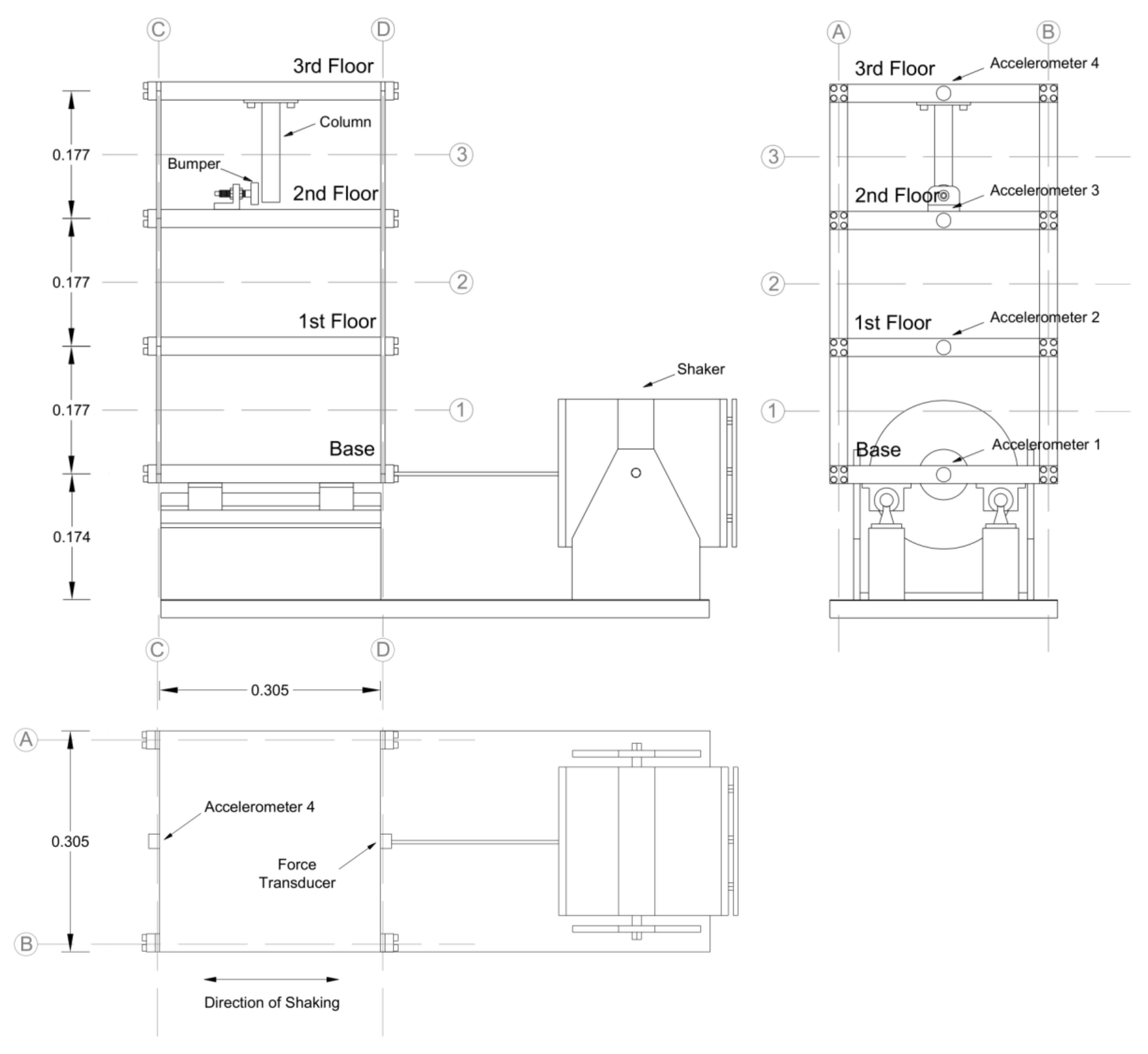
A three-story structure was selected as the damage detection test stand in the experimental procedure, as shown in Figure 5. Each layer is connected by four aluminum columns (17.7 × 2.5 × 0.6 cm) with aluminum plates at the top and bottom (30.5 × 30.5 × 2.5 cm), forming a four-degree-of-freedom system. It can be seen from Figure 5 that there was a central column (15.0 × 2.5 × 2.5 cm) suspended from the top level and a buffer, which can adjust the narrow space between buffer and central column. It could change the degree of nonlinearity, and the structure allowed the track to slide in the x-axis direction only.
The shaker that provided excitation to the bottom was mounted on the substrate. A force sensor with a sensitivity of 2.2 mV/N was mounted at the end of the probe to measure the input force from the shaker. The sampling interval was set to 3.1 ms, and the sampling frequency was set to 322.58 H. In this study, State#14, namely (change gap = 0.10 mm, apply 1.2 kg weight to the first layer), is selected as the experimental object where Channel 2, Channel 3, Channel 4, and Channel 5 denoted the positions of the accelerometers and Channel 1 denoted the position of the shaker in Figure 6. The four data sets collected from four acceleration are selected to verify the effectiveness of the proposed method predicting missing data.
To describe the essential characteristics of the four acceleration data, four statistical indicators, including total sample size, mean, maximum and minimum values, and standard deviation, are selected for the four data sets. The result is shown in Table 1.
In this table, A_1, A_2, A_3, and A_4 represent collected data from the accelerometer of Channel 2, Channel 3, Channel 4, Channel 5. Figure 7 shows a curve picture of collected acceleration data.
First, each data set is divided into two parts, 80% data set is used as a training set, and the remaining 20% data set is used as a test set. As seen from Figure 8, solid boxes, as input data, are used to predict the value at the next step. Dashed boxes represent the missing data during measured signal data. For two points missing data, each input and output pair consists of 324 samples, including 322 input samples (e.g., 1 to 322) and two output samples (e.g., 323–324), namely missing data. Then, the input-output pairs are fed into the EMD-BiGRU model for training, and then a predicted model with two missing points can be achieved. When a measured signal occurs two missing points, the model can be used to predict the missing data. Similarly, EMD-BiGRU models predicting different lengths (5, 10, 20 missing data) can be achieved to tackle the problem of missing data with different lengths.
3.2. Acceleration Decomposition Based on EMD
EMD algorithm is used to decompose the raw acceleration data into several IMF components and one residual res where different components have different trends and characteristics, representing different features of the fluctuations of the raw acceleration data. The decomposition results for the four data sets are shown in Figure 9, Figure 10, Figure 11 and Figure 12. For every picture, the horizontal axis is the time point, and the vertical axis is the decomposition value. All components are listed in order of extraction from highest to lowest frequency.
As can be seen from Figure 9, Figure 10, Figure 11 and Figure 12, the first few IMF components are random components with an insignificant pattern of variation. The middle components have the fluctuating feature to reflect more features of the original data. The last few IMF components with low-frequency reflect the slow change process of acceleration. The last component is the residual, which reflects the overall trend of the acceleration data.
3.3. Parameters Setting of Different Algorithms
In terms of hardware, a server with 128G RAM, 2048 GB hard disk space is selected. The type of GPU is NVIDIA Tesla K40c, and the type of CPU is Intel Xeon E5. For the experimental software, the Keras 2.4.3 tool based on Tensorflow version 2.4.0 under python is selected as the development conditions for the deep learning methods. The parameters of the seven algorithms are as follows:
The parameters setting of EMD-BiGUR, EMD-GRU, BiGRU, and GRU are as follows:
EMD-BiGUR: The raw acceleration data and decomposed subsequence decomposed by EMD are inputted into BiGRU algorithms. BiGRU used Tanh activation function, and the neurons number is 60. Then, the BiGRU layer linked two fully connected layers, whose neuron sizes are 512 and 256.
EMD-GRU: The raw acceleration data and decomposed subsequence decomposed by EMD are inputted into GRU algorithms. The activation function of Tanh is used for the GRU layer with 60 neurons. The GRU layer linked two fully connected layers whose neuron sizes are 512 and 256.
BiGRU: The BiGRU used Tanh’s activation function, and the number of neurons in the hidden layer is 60. Then, the BiGRU layer linked two fully connected layers whose neuron sizes are 512 and 256.
GRU: The GRU layer used Tanh’s activation function, and the number of neurons in the hidden layer is 60. The GRU layer linked two fully connected layers whose neuron sizes are 512 and 256.
The common parameter settings for the mentioned algorithms, such as EMD-BiGUR, EMD-GRU, BiGRU, GRU, are as follows: The initial learning rate is 0.01, and the optimizer is selected Adma. The algorithms adopt 300 epochs iteration. The mean square error (MSE) is used for the loss function, and the Mini-Batch is set to 128.
The parameters setting for machine learning methods such as GBR, RFR, and SVR are set as follows:
Gradient Boosting Regressor (GBR): the learning rate is 0.1, and the maximum depth is 6. The range of maximum number of is set to [10,100], which is optimized by using a grid search
Random Forest Regressor (RFR): The range of maximum number of is set to [10,100], which is optimized by using a grid search
Support vector regressor (SVR): a Gaussian RBF function is used as the SVR kernel function, and a grid search is used to determine the penalty parameters and kernel parameters . The search range and are [10−4, 104] and [2−4,24], respectively.
4. Analysis of Predicted Results
To evaluate the superiority of the proposed EMD-BiGRU algorithm, six algorithms, including EMD-GRU, BiGRU, GRU, GBR, RFR, and SVR, were selected for analysis. BiGRU, GRU, GBR, RFR, and SVR models are single-predicted methods that use raw acceleration data to predict missing data. EMD-BiGRU, EMD-GRU are hybrid predicted methods based on EMD decomposition. The decomposed subseries and raw acceleration data are inputted into hybrid predicted methods together to forecast missing data. To verify the effectiveness of different algorithms, four acceleration data are located on different locations of a three-story structure are tested by using different methods, such as EMD-BiGRU, EMD-GRU, BiGRU, GRU, GBR, RFR, SVR algorithms in Table 2. In addition, point 5 represents that 5 points are missing for raw data sets.
Table 2 represents the prediction results for four data sets (A_1, A_2, A_3, and A_4) using different methods. The bold number indicates that the method has the best performance in the corresponding data sets. It can be seen from Table 3 that the EMD-BiGRU has the minimum values of MSE, RMSE, MAE, and the maximum value of R2, compared with the other six methods. To be specific, for A_1 data sets, compared with the EMD-GRU algorithm, the EMD-BiGRU reduces 0.0151, 0.0499, and 0.0389 in MSE, RMSE, and MAE, respectively, and increases 0.0536 in R2. EMD-BiGRU reduces 0.0151, 0.0499, and 0.0389 in MSE, RMSE, and MAE, respectively, and an increase of 0.9433 in the R2, compared with the BiGRU in A_1 data sets. Moreover, the EMD-BiGRU has lower MSE, RMSE, MAE, and higher R2 than the machine learning models GBR, RFR, SVR in A_1 data sets.
In addition, The MSE values of the EMD-BiGRU for A_1, A_2, A_3, and A_4 are 0.0160, 0.0065, 0.0040, and 0.0041, respectively. Compared to the comparative model’s minimum MSE, it reduces by 0.0151, 0.0032, 0.0015, and 0.0123 using the EMD-BiGRU method. Compared to the comparative model’s minimum RMSE, it reduces by 0.0499, 0.0179, 0.0107, and 0.0637, respectively. Compared to comparative model’s minimum MAE, it increased by 0.0389, 0.0130, 0.0079, 0.0442, respectively. It increased by 0.0536, 0.0155, 0.0067, 0.0812, compared to its comparative model’s maximum R2, respectively. In summary, GRU, BiGRU, etc., deep learning algorithms outperform GBR, RFR, SVR machine learning methods on predicted capability, which indicates the superiority of deep learning in dealing with temporal sequences. EMD-based hybrid models such as EMD-GRU, EMD-BiGRU have lower errors in MSE, RMSE, MAE compared with single models such as GRU, BiGRU, which indicates the effectiveness of the EMD method.
Figure 13 shows the comparison curves between predicted and actual values for the four data sets using different algorithms. Considering that the number of predicted data is so long, this study selected part of the predicted result to show (50 points). Experimental results indicate that EMD-BiGRU can better capture the characteristics of acceleration data and has a better prediction for missing points.
Table 3 shows the predicted results of the A_1 data set using different models, and the predicted points include 5, 10, 15, and 20. It can be seen from Table 3 that the accuracy of most algorithms can decrease with the increasing missing points. For example, the machine learning methods GBR, RFR, and SVR drop a little faster, indicating that these algorithms are less capable of extracting temporal features of acceleration data. Moreover, the single model BiGRU GRU has better prediction than the machine learning methods, but its robustness is poor. The hybrid EMD-based models such as EMD-BiGRU, EMD-GRU are more robust and have suitable prediction results. In addition, the EMD-BiGRU has lower MSE, RMSE, MAE compared with EMD-GRU, which indicates that the predicted ability of EMD-BiGRU is more superior. To be specific, the EMD-BiGRU model only reduces by 5.76% in R2 for predicting points from 5 to 20, which represents that the EMD-BiGRU has a minor loss. For A_2, A_3, and A_4 data sets, the predicted results using different models can be seen in Table A1, Table A2 and Table A3.
Figure 14 shows predicted results on A_1, A_2, A_3, and A_4 by using different algorithms. It can be seen that EMD-BiGRU can better capture the characteristics of acceleration data and has a better prediction for missing points. For A_2, A_3, and A_4 data sets, the predicted results using different models can be seen in Figure A1, Figure A2 and Figure A3.
5. Effectiveness of the EMD-BiGRU for Data Loss Recovery under Different Structural Conditions
5.1. Data Description
To verify the effectiveness of the proposed method under different structural conditions, a three-story building structure is used for the study. A detailed description of the three-story building structure refers to Section 3.1.
Table 4 shows the different structural conditions of the three-story building structure. Four structural conditions are selected in this study. For each structural condition, the collected system provides a band-limited random excitation in the range of 20–150 Hz acting on the three-story structure. Figure 15 and Figure 16 show the detailed description of different structural conditions. For State#12, the gap between the bumper and the suspended column is set to 0.2 mm, which can be simulation impact-induced damage. State#16 is designed for mass changes and impact-induced damage. State#21 and State#23 accounts for structural damage due to stiffness reduction.
5.2. Experimental Analysis
In this case study, all experiments are performed on the same hardware and software environment. Table 5 shows a comparison of the different structural conditions using the EMD-BiGRU algorithm. It should be seen that the proposed method achieves high accuracy and robustness. Specifically, the EMD-BiGRU achieves 0.0118%, 0.1084%, 0.0842%, and 95.81% in MSE, RMSE, MAE, and R2 for 10 points of Case 1. With increasing missing data, the R2 of Case 1 are 95.81% (10 points), 94.70% (15 points), 91.57% (20 points), respectively, which shows EMD-BiGRU has high accuracy. In addition, the proposed method has robustness due to the R2 value dropping slowly. For other structural conditions, Cases two, three, and four, the EDM-BiGRU has a similar result, and the R2 value is more than 0.9. Therefore, this result shows that the proposed method has high data recovery ability in civil structures.
6. Conclusions and Future Work
This study proposed the EMD-BiGRU method for predicting missing data where the EMD algorithm decomposes acceleration data into many subseries reflecting structural model information, and BiGRU effectively extracts the pre-post correlations of subsequence decomposed by acceleration. Specifically, the proposed EMD-BiGRU method can decompose raw measured signal data into several IMFs and a residual. Every IMF can reflect the complex changes of the measured data in dimensions. Then, the imputation ability of the proposed EMD-BiGRU is evaluated using acceleration monitoring data collected from a three-story building structure. Compared with traditional methods such as EMD-GRU, BiGRU, GRU, GBR, RFR, and SVR, experimental results on A_1, A_2, A_3, and A_4 show that EMD-BiGRU has high accuracy in predicting missing points 5, 10, 15, 20. The main findings of the present study are summarized as follows.
- (1)
- In recognition of the influence of EMD, the EMD-BiGRU and single models such as BiGRU, GRU, GBR, RFR, and SVR are investigated. The results show that the proposed EMD-BiGRU method achieves better performance for data imputation and demonstrates that the proposed method effectively captures the dynamic temporal characteristics of acceleration data.
- (2)
- With the increasing missing data, the data recovery ability of most algorithms could decrease. EMD-BiGRU has lower errors in MSE, RMSE, and MAE than single algorithms such as GRU, GBR, and BiGRU. It indicates that the proposed method has strong robustness and can be promoted on a large scale in practical applications
- (3)
- For different structural conditions of a three-story building, the EMD-BiGRU exhibits better data imputation performance. It shows that EMD-BiGRU, as a flexible and data-driven method, is effective for mining measured acceleration data.
- (4)
- One of the limitations of this study is that EMD-BiGRU is tested using original acceleration data without considering the effect of noise. In future work, raw acceleration data with the noises are considered to solve the imputation of the missing data. Another future research direction is that the extension of EMD to tackle missing data should be studied in the future.
Author Contributions
Funding acquisition, investigation, data curation, D.L.; software, validation, visualization, Y.B.; data curation, visualization, Writing—original draft, Y.H. data curation, methodology, supervision, validation, L.Z. All authors have read and agreed to the published version of the manuscript.
Funding
The work described in this paper was supported by the Foundation project of Scientific Research Platform of Hechuan for Chengdu-Chongqing Economic Area Research Base and the Teaching Reform Project of School (Grant No. 19CRKXJJG05), the Scientific Research Program of Chongqing College of Humanities, Science & Technology (Grant No. CQRKZX2020003).
Institutional Review Board Statement
Not applicable.
Informed Consent Statement
Not applicable.
Acknowledgments
The authors would like to thank the anonymous reviewers for their valuable comments on the manuscript.
Conflicts of Interest
The authors declare that no conflict interest for the present study was found.
Appendix A
The predicted results for A_2 data sets using seven algorithms, including EMD-BiGRU, EMD-GRU, BiGRU, GRU, GBR, RFR, SVR, are shown in Table A1.

Table A1.
Comparison results for data set A_2 using different algorithms.
| data set | Point | Metrics | EMD-BiGRU | EMD-GRU | BiGRU | GRU | GBR | RFR | SVR |
|---|---|---|---|---|---|---|---|---|---|
| A_2 | 5 | MSE | 0.0065 | 0.0097 | 0.0249 | 0.0249 | 0.0573 | 0.0669 | 0.0429 |
| 5 | RMSE | 0.0808 | 0.0987 | 0.1579 | 0.1579 | 0.2394 | 0.2587 | 0.2070 | |
| 5 | MAE | 0.0609 | 0.0739 | 0.1175 | 0.1182 | 0.1859 | 0.2010 | 0.1595 | |
| 5 | R2 | 96.85% | 95.30% | 87.97% | 87.96% | 72.35% | 67.72% | 79.32% | |
| A_2 | 10 | MSE | 0.0054 | 0.0083 | 0.0156 | 0.0203 | 0.0841 | 0.0935 | 0.0679 |
| 10 | RMSE | 0.0731 | 0.0910 | 0.1250 | 0.1424 | 0.2900 | 0.3058 | 0.2606 | |
| 10 | MAE | 0.0567 | 0.0711 | 0.0957 | 0.1090 | 0.2259 | 0.2386 | 0.2009 | |
| 10 | R2 | 97.44% | 96.03% | 92.51% | 90.29% | 59.68% | 55.17% | 67.45% | |
| A_2 | 15 | MSE | 0.0073 | 0.0129 | 0.0200 | 0.0181 | 0.0919 | 0.0992 | 0.0777 |
| 15 | RMSE | 0.0856 | 0.1136 | 0.1415 | 0.1345 | 0.3031 | 0.3149 | 0.2787 | |
| 15 | MAE | 0.0674 | 0.0887 | 0.1096 | 0.1049 | 0.2375 | 0.2476 | 0.2170 | |
| 15 | R2 | 96.48% | 93.78% | 90.36% | 91.29% | 55.77% | 52.25% | 62.60% | |
| A_2 | 20 | MSE | 0.0047 | 0.0086 | 0.0829 | 0.0192 | 0.1026 | 0.1091 | 0.0904 |
| 20 | RMSE | 0.0684 | 0.0929 | 0.2880 | 0.1384 | 0.3203 | 0.3302 | 0.3007 | |
| 20 | MAE | 0.0534 | 0.0727 | 0.2233 | 0.1079 | 0.2524 | 0.2609 | 0.2351 | |
| 20 | R2 | 97.76% | 95.87% | 60.33% | 90.84% | 50.92% | 47.84% | 56.76% |
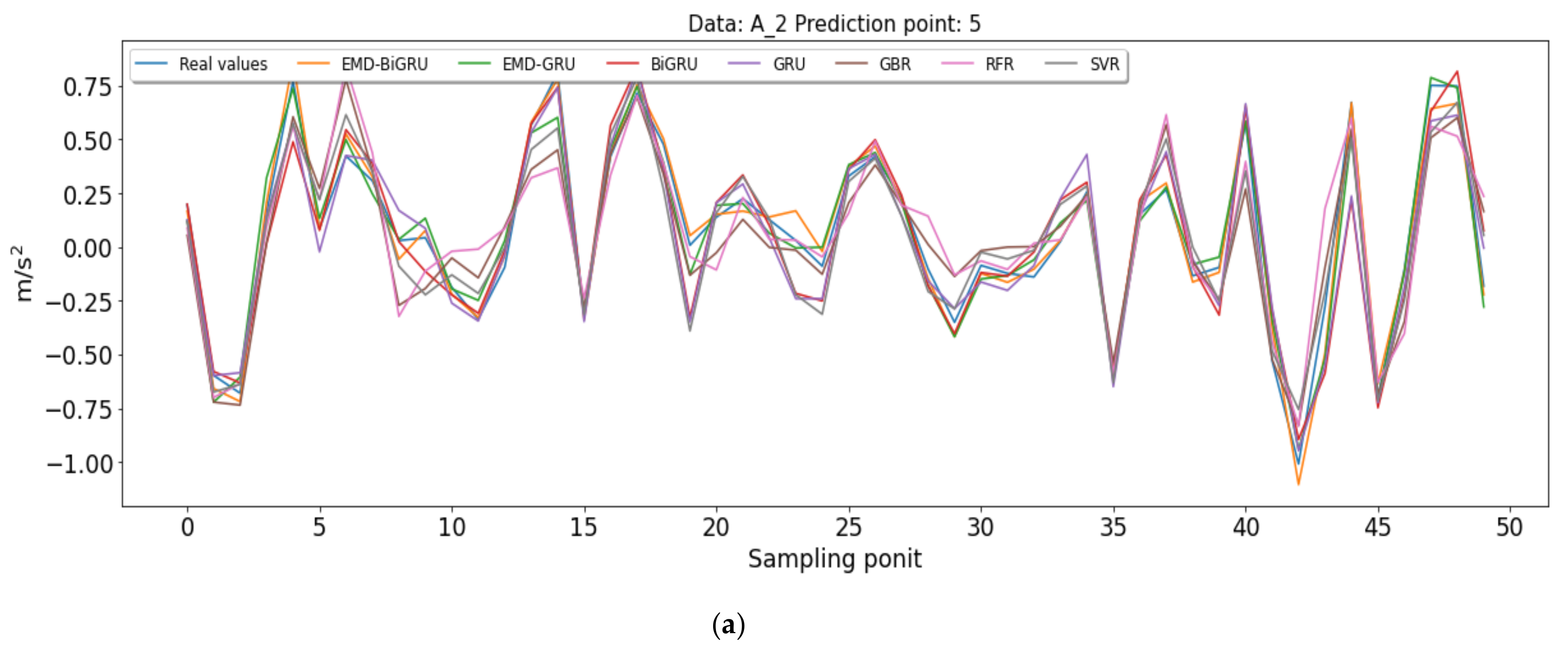
Figure A1 shows the prediction results for the A_2 data set using different comparison algorithms.
Figure A1.
Comparisons results for different data sets using various algorithms. (a) Comparisons of predicted results for the A_2 data set using different algorithms (points 5). (b) Comparisons of predicted results for the A_2 data set using different algorithms (points 10). (c) Comparisons of predicted results for the A_2 data set using different algorithms (points 15). (d) Comparisons of predicted results for the A_2 data set using different algorithms (points 20).


The predicted results for A_3 data sets using seven algorithms, including EMD-BiGRU, EMD-GRU, BiGRU, GRU, GBR, RFR, SVR, which are shown in Table A2.
Table A2.
Comparison results for data set A_3 using different algorithms.
| data set | Point | Metrics | EMD-BiGRU | EMD-GRU | BiGRU | GRU | GBR | RFR | SVR |
|---|---|---|---|---|---|---|---|---|---|
| A_3 | 5 | MSE | 0.004 | 0.0055 | 0.0124 | 0.0114 | 0.0299 | 0.0321 | 0.0244 |
| 5 | RMSE | 0.0634 | 0.0741 | 0.1115 | 0.1066 | 0.173 | 0.179 | 0.1563 | |
| 5 | MAE | 0.0458 | 0.0537 | 0.0798 | 0.0763 | 0.1329 | 0.1365 | 0.12 | |
| 5 | R2 | 98.15% | 97.48% | 94.29% | 94.78% | 86.26% | 85.27% | 88.78% | |
| A_3 | 10 | MSE | 0.0028 | 0.0056 | 0.0381 | 0.0376 | 0.0575 | 0.0612 | 0.0494 |
| 10 | RMSE | 0.0526 | 0.0751 | 0.1953 | 0.1939 | 0.2399 | 0.2473 | 0.2223 | |
| 10 | MAE | 0.0396 | 0.057 | 0.141 | 0.1393 | 0.1821 | 0.1873 | 0.1674 | |
| 10 | R2 | 98.71% | 97.36% | 82.15% | 82.4% | 73.06% | 71.37% | 76.86% | |
| A_3 | 15 | MSE | 0.0039 | 0.0053 | 0.0195 | 0.0609 | 0.0799 | 0.0825 | 0.0724 |
| 15 | RMSE | 0.0626 | 0.0726 | 0.1396 | 0.2468 | 0.2826 | 0.2872 | 0.2691 | |
| 15 | MAE | 0.0485 | 0.0563 | 0.1065 | 0.1803 | 0.2151 | 0.2192 | 0.2031 | |
| 15 | R2 | 98.18% | 97.55% | 90.94% | 71.67% | 62.84% | 61.62% | 66.32% | |
| A_3 | 20 | MSE | 0.0043 | 0.0059 | 0.0707 | 0.0777 | 0.0934 | 0.0954 | 0.0872 |
| 20 | RMSE | 0.0655 | 0.0766 | 0.2658 | 0.2787 | 0.3055 | 0.3089 | 0.2952 | |
| 20 | MAE | 0.0507 | 0.0596 | 0.1991 | 0.2075 | 0.2341 | 0.2371 | 0.2245 | |
| 20 | R2 | 97.99% | 97.26% | 66.98% | 63.69% | 56.37% | 55.41% | 59.26% |
Figure A2 shows the prediction results for data set A_3 using different comparison algorithms.
Figure A2.
Comparisons results for different data sets using various algorithms. (a) Comparisons of predicted results for the A_3 data set using different algorithms (points 5). (b) Comparisons of predicted results for the A_3 data set using different algorithms (points 10). (c) Comparisons of predicted results for the A_3 data set using different algorithms (points 15). (d)Comparisons of predicted results for the A_3 data set using different algorithms (points 20).


The predicted results for A_4 data sets using seven algorithms, including EMD-BiGRU, EMD-GRU, BiGRU, GRU, GBR, RFR, SVR, which are shown in Table A3.
Table A3.
Comparison results for data set A_4 using different algorithms.
| data set | Point | Metrics | EMD-BiGRU | EMD-GRU | BiGRU | GRU | GBR | RFR | SVR |
|---|---|---|---|---|---|---|---|---|---|
| A_4 | 5 | MSE | 0.0041 | 0.0164 | 0.0187 | 0.0180 | 0.0440 | 0.0495 | 0.035 |
| 5 | RMSE | 0.0644 | 0.1281 | 0.1367 | 0.1343 | 0.2097 | 0.2226 | 0.187 | |
| 5 | MAE | 0.0470 | 0.0912 | 0.0957 | 0.0938 | 0.1597 | 0.1690 | 0.1414 | |
| 5 | R2 | 97.26% | 89.14% | 87.64% | 88.07% | 70.91% | 67.21% | 76.87% | |
| A_4 | 10 | MSE | 0.0032 | 0.0039 | 0.0518 | 0.0107 | 0.0728 | 0.0770 | 0.0647 |
| 10 | RMSE | 0.0562 | 0.0622 | 0.2277 | 0.1036 | 0.2698 | 0.2774 | 0.2543 | |
| 10 | MAE | 0.0427 | 0.0471 | 0.1649 | 0.0780 | 0.2063 | 0.2130 | 0.192 | |
| 10 | R2 | 97.92% | 97.45% | 65.82% | 92.92% | 52.01% | 49.25% | 57.35% | |
| A_4 | 15 | MSE | 0.0033 | 0.0048 | 0.0739 | 0.0734 | 0.0844 | 0.088 | 0.0784 |
| 15 | RMSE | 0.0578 | 0.0691 | 0.2718 | 0.2709 | 0.2905 | 0.2966 | 0.2801 | |
| 15 | MAE | 0.0447 | 0.0539 | 0.2029 | 0.2028 | 0.2252 | 0.2305 | 0.215 | |
| 15 | R2 | 97.76% | 96.8% | 50.46% | 50.77% | 43.38% | 41.0% | 47.39% | |
| A_4 | 20 | MSE | 0.0038 | 0.0053 | 0.0841 | 0.0102 | 0.0931 | 0.0960 | 0.0883 |
| 20 | RMSE | 0.0618 | 0.0727 | 0.2901 | 0.1008 | 0.3052 | 0.3099 | 0.2971 | |
| 20 | MAE | 0.0477 | 0.0566 | 0.2198 | 0.0771 | 0.2370 | 0.2411 | 0.2286 | |
| 20 | R2 | 97.45% | 96.47% | 43.75% | 93.21% | 37.74% | 35.81% | 40.99% |
Figure A3 shows the prediction results for data set A_4 using different comparison algorithms.
Figure A3.
Comparisons results for different data sets using various algorithms. (a) Comparisons of predicted results for the A_4 data set using different algorithms (points 5). (b) Comparisons of predicted results for the A_4 data set using different algorithms (points 10). (c) Comparisons of predicted results for the A_4 data set using different algorithms (points 15). (d) Comparisons of predicted results for the A_4 data set using different algorithms (points 20).


References
- Annamdas, V.G.M.; Bhalla, S.; Soh, C.K. Applications of Structural Health Monitoring Technology in Asia. Struct. Health Monit. 2017, 16, 324–346. [Google Scholar] [CrossRef]
- Li, H.; Ou, J. The State of the Art in Structural Health Monitoring of Cable-Stayed Bridges. J. Civ. Struct. Health Monit. 2016, 6, 43–67. [Google Scholar] [CrossRef]
- Nagayama, T.; Sim, S.H.; Miyamori, Y.; Spencer, B.F., Jr. Issues in Structural Health Monitoring Employing Smart Sensors. Smart Struct. Syst. 2007, 3, 299–320. [Google Scholar] [CrossRef] [Green Version]
- Bao, Y.; Yu, Y.; Li, H.; Mao, X.; Jiao, W.; Zou, Z.; Ou, J. Compressive Sensing-Based Lost Data Recovery of Fast-Moving Wireless Sensing for Structural Health Monitoring: Lost Data Recovery for Fast-Moving Wireless Sensing. Struct. Control Health Monit. 2015, 22, 433–448. [Google Scholar] [CrossRef]
- Huang, Y.; Beck, J.L.; Wu, S.; Li, H. Bayesian Compressive Sensing for Approximately Sparse Signals and Application to Structural Health Monitoring Signals for Data Loss Recovery. Probabilistic Eng. Mech. 2016, 46, 62–79. [Google Scholar] [CrossRef] [Green Version]
- Hong, Y.H.; Kim, H.-K.; Lee, H.S. Reconstruction of Dynamic Displacement and Velocity from Measured Accelerations Using the Variational Statement of an Inverse Problem. J. Sound Vib. 2010, 329, 4980–5003. [Google Scholar] [CrossRef]
- Bao, Y.; Li, H.; Sun, X.; Yu, Y.; Ou, J. Compressive Sampling–Based Data Loss Recovery for Wireless Sensor Networks Used in Civil Structural Health Monitoring. Struct. Health Monit. 2013, 12, 78–95. [Google Scholar] [CrossRef]
- Zou, Z.; Bao, Y.; Li, H.; Spencer, B.F.; Ou, J. Embedding Compressive Sensing-Based Data Loss Recovery Algorithm into Wireless Smart Sensors for Structural Health Monitoring. IEEE Sens. J. 2015, 15, 797–808. [Google Scholar] [CrossRef]
- Liu, G.; Mao, Z.; Todd, M.; Huang, Z. Damage Assessment with State-Space Embedding Strategy and Singular Value Decomposition under Stochastic Excitation. Struct. Health Monit. 2014, 13, 131–142. [Google Scholar] [CrossRef]
- Wan, H.-P.; Ni, Y.-Q. Bayesian Multi-Task Learning Methodology for Reconstruction of Structural Health Monitoring Data. Struct. Health Monit. 2019, 18, 1282–1309. [Google Scholar] [CrossRef] [Green Version]
- Yang, Y.; Nagarajaiah, S. Harnessing Data Structure for Recovery of Randomly Missing Structural Vibration Responses Time History: Sparse Representation versus Low-Rank Structure. Mech. Syst. Signal Process. 2016, 74, 165–182. [Google Scholar] [CrossRef]
- Choi, S.; Kwon, E.; Kim, Y.; Hong, K.; Park, H. A Practical Data Recovery Technique for Long-Term Strain Monitoring of Mega Columns during Construction. Sensors 2013, 13, 10931–10943. [Google Scholar] [CrossRef]
- He, J.; Guan, X.; Liu, Y. Structural Response Reconstruction Based on Empirical Mode Decomposition in Time Domain. Mech. Syst. Signal Process. 2012, 28, 348–366. [Google Scholar] [CrossRef]
- Luo, Y.F.; Ye, Z.W.; Guo, X.N.; Qiang, X.H.; Chen, X.M. Data Missing Mechanism and Missing Data Real-Time Processing Methods in the Construction Monitoring of Steel Structures. Adv. Struct. Eng. 2015, 18, 585–601. [Google Scholar] [CrossRef]
- Zhang, Z.; Luo, Y. Restoring Method for Missing Data of Spatial Structural Stress Monitoring Based on Correlation. Mech. Syst. Signal Process. 2017, 91, 266–277. [Google Scholar] [CrossRef]
- Hua, Y.; Zhao, Z.; Li, R.; Chen, X.; Liu, Z.; Zhang, H. Deep Learning with Long Short-Term Memory for Time Series Prediction. IEEE Commun. Mag. 2019, 57, 114–119. [Google Scholar] [CrossRef] [Green Version]
- Deng, Y.; Jia, H.; Li, P.; Tong, X.; Qiu, X.; Li, F. A Deep Learning Methodology Based on Bidirectional Gated Recurrent Unit for Wind Power Prediction. In Proceedings of the 2019 14th IEEE Conference on Industrial Electronics and Applications (ICIEA), Xi’an, China, 19–21 June 2019; pp. 591–595. [Google Scholar]
- Li, X.; Zhuang, W.; Zhang, H. Short-Term Power Load Forecasting Based on Gate Recurrent Unit Network and Cloud Computing Platform. In Proceedings of the 4th International Conference on Computer Science and Application Engineering, Sanya, China, 20 October 2020; pp. 1–6. [Google Scholar]
- Rosafalco, L.; Manzoni, A.; Mariani, S.; Corigliano, A. Fully Convolutional Networks for Structural Health Monitoring through Multivariate Time Series Classification. Adv. Model. Simul. Eng. Sci. 2020, 7, 38. [Google Scholar] [CrossRef]
- Liu, H.; Ding, Y.-L.; Zhao, H.-W.; Wang, M.-Y.; Geng, F.-F. Deep Learning-Based Recovery Method for Missing Structural Temperature Data Using LSTM Network. Struct. Monit. Maint. 2020, 7, 109–124. [Google Scholar] [CrossRef]
- Fan, G.; Li, J.; Hao, H. Lost Data Recovery for Structural Health Monitoring Based on Convolutional Neural Networks. Struct. Control. Health Monit. 2019, 26, e2433. [Google Scholar] [CrossRef]
- Abd Elaziz, M.; Dahou, A.; Abualigah, L.; Yu, L.; Alshinwan, M.; Khasawneh, A.M.; Lu, S. Advanced Metaheuristic Optimization Techniques in Applications of Deep Neural Networks: A Review. Neural Comput. Appl. 2021. [Google Scholar] [CrossRef]
- Abualigah, L.; Yousri, D.; Abd Elaziz, M.; Ewees, A.A.; Al-qaness, M.A.A.; Gandomi, A.H. Aquila Optimizer: A Novel Meta-Heuristic Optimization Algorithm. Comput. Ind. Eng. 2021, 157, 107250. [Google Scholar] [CrossRef]
- Wang, Z.-C.; Ren, W.-X.; Chen, G. Time–Frequency Analysis and Applications in Time-Varying/Nonlinear Structural Systems: A State-of-the-Art Review. Adv. Struct. Eng. 2018, 21, 1562–1584. [Google Scholar] [CrossRef]
- Rezaei, D.; Taheri, F. Damage Identification in Beams Using Empirical Mode Decomposition. Struct. Health Monit. 2011, 10, 261–274. [Google Scholar] [CrossRef]
- Gao, X.; Li, X.; Zhao, B.; Ji, W.; Jing, X.; He, Y. Short-Term Electricity Load Forecasting Model Based on EMD-GRU with Feature Selection. Energies 2019, 12, 1140. [Google Scholar] [CrossRef] [Green Version]
- Figueiredo, E.; Park, G.; Figueiras, J.; Farrar, C.; Worden, K. Structural Health Monitoring Algorithm Comparisons Using Standard Data Sets; Los Alamos National Lab.: Los Alamos, NM, USA, 2009; LA-14393, 961604. [Google Scholar]
- Gan, D.; Wang, Y.; Zhang, N.; Zhu, W. Enhancing Short-term Probabilistic Residential Load Forecasting with Quantile Long–Short-term Memory. J. Eng. 2017, 2017, 2622–2627. [Google Scholar] [CrossRef]
- Dong, S.; Yuan, M.; Wang, Q.; Liang, Z. A Modified Empirical Wavelet Transform for Acoustic Emission Signal Decomposition in Structural Health Monitoring. Sensors 2018, 18, 1645. [Google Scholar] [CrossRef] [Green Version]
- Li, A.; Cheng, L. Research on A Forecasting Model of Wind Power Based on Recurrent Neural Network with Long Short-Term Memory. In Proceedings of the 2019 22nd International Conference on Electrical Machines and Systems (ICEMS), Harbin, China, 11–14 August 2019; pp. 1–4. [Google Scholar]
- Yang, J.; Zhang, L.; Chen, C.; Li, Y.; Li, R.; Wang, G.; Jiang, S.; Zeng, Z. A Hierarchical Deep Convolutional Neural Network and Gated Recurrent Unit Framework for Structural Damage Detection. Inf. Sci. 2020, 540, 117–130. [Google Scholar] [CrossRef]
- Liu, C.; Qi, J. Text Sentiment Analysis Based on ResGCNN. In Proceedings of the 2019 Chinese Automation Congress (CAC), Hangzhou, China, 22–24 November 2019; pp. 1604–1608. [Google Scholar]
- Singh, P.; Dwivedi, P. Integration of New Evolutionary Approach with Artificial Neural Network for Solving Short Term Load Forecast Problem. Appl. Energy 2018, 217, 537–549. [Google Scholar] [CrossRef]
- Zhao, Y.; Ye, L.; Pinson, P.; Tang, Y.; Lu, P. Correlation-Constrained and Sparsity-Controlled Vector Autoregressive Model for Spatio-Temporal Wind Power Forecasting. IEEE Trans. Power Syst. 2018, 33, 5029–5040. [Google Scholar] [CrossRef] [Green Version]
- Mashaly, A.F.; Alazba, A.A.; Al-Awaadh, A.M.; Mattar, M.A. Predictive Model for Assessing and Optimizing Solar Still Performance Using Artificial Neural Network under Hyper Arid Environment. Sol. Energy 2015, 118, 41–58. [Google Scholar] [CrossRef]
Figure 1.
EMD decomposition of acceleration data for a three-story building structure.

Figure 2.
GRU structure diagram.

Figure 3.
BiGRU structural diagram.

Figure 4.
Flow chart of EMD-BiGRU prediction.

Figure 5.
The three-story building structure.

Figure 6.
Position of accelerator sensor installed structure.

Figure 7.
Acceleration data set collected from the three-story structure.

Figure 8.
Input and output of the proposed model.

Figure 9.
Results of decomposition for A_1 acceleration data sets.

Figure 10.
Results of decomposition for A_2 acceleration data sets.

Figure 11.
Results of decomposition for A_3 acceleration data sets.

Figure 12.
Results of decomposition for A_4 acceleration data sets.

Figure 13.
Comparisons results for different data sets using various algorithms. (a) Comparisons of predicted results for the A_1 data set using different algorithms. (b) Comparisons of predicted results for the A_2 data set using different algorithms. (c) Comparisons of predicted results for the A_3 data set using different algorithms. (d) Comparisons of predicted results for the A_4 data set using different algorithms.


Figure 14.
Comparisons results for different data sets using various algorithms. (a) Comparisons of predicted results for the A_1 data set using different algorithms (points 5). (b) Comparisons of predicted results for the A_1 data set using different algorithms (points 10). (c) Comparisons of predicted results for the A_1 data set using different algorithms (points 15). (d) Comparisons of predicted results for the A_1 data set using different algorithms (points 20).


Figure 15.
Dimensions information of the three-story building structure.

Figure 16.
Descriptions of the three-story building structure.

Table 1.
Statistical indicators for the four acceleration data.
| data set | A_1 | A_2 | A_3 | A_4 |
|---|---|---|---|---|
| Number of samples | 8192 | 8192 | 8192 | 8192 |
| Mean | 0.000009 | 0.000073 | 0.000304 | −0.000018 |
| Standard deviation | 0.5366 | 0.4556 | 0.4593 | 0.3856 |
| Min | −2.0286 | −1.8864 | −1.7249 | −1.7085 |
| Max | 1.9513 | 2.2541 | 2.1054 | 1.4282 |
Table 2.
Comparison results of different models for the data set.
| data set | Point | Metrics | EMD-BiGRU | EMD-GRU | BiGRU | GRU | GBR | RFR | SVR |
|---|---|---|---|---|---|---|---|---|---|
| A_1 | 5 | MSE | 0.0160 | 0.0311 | 0.1088 | 0.1005 | 0.1529 | 0.1652 | 0.1292 |
| 5 | RMSE | 0.1264 | 0.1763 | 0.3298 | 0.3170 | 0.3910 | 0.4064 | 0.3595 | |
| 5 | MAE | 0.0942 | 0.1331 | 0.2525 | 0.2389 | 0.3108 | 0.3232 | 0.2825 | |
| 5 | R2 | 94.33% | 88.97% | 61.40% | 64.34% | 45.73% | 41.39% | 54.14% | |
| A_2 | 5 | MSE | 0.0065 | 0.0097 | 0.0249 | 0.0249 | 0.0573 | 0.0669 | 0.0429 |
| 5 | RMSE | 0.0808 | 0.0987 | 0.1579 | 0.1579 | 0.2394 | 0.2587 | 0.2070 | |
| 5 | MAE | 0.0609 | 0.0739 | 0.1175 | 0.1182 | 0.1859 | 0.2010 | 0.1595 | |
| 5 | R2 | 96.85% | 95.30% | 87.97% | 87.96% | 72.35% | 67.72% | 79.32% | |
| A_3 | 5 | MSE | 0.0040 | 0.0055 | 0.0124 | 0.0114 | 0.0299 | 0.0321 | 0.0244 |
| 5 | RMSE | 0.0634 | 0.0741 | 0.1115 | 0.1066 | 0.173 | 0.179 | 0.1563 | |
| 5 | MAE | 0.0458 | 0.0537 | 0.0798 | 0.0763 | 0.1329 | 0.1365 | 0.1200 | |
| 5 | R2 | 98.15% | 97.48% | 94.29% | 94.78% | 86.26% | 85.27% | 88.78% | |
| A_4 | 5 | MSE | 0.0041 | 0.0164 | 0.0187 | 0.0180 | 0.0440 | 0.0495 | 0.0350 |
| 5 | RMSE | 0.0644 | 0.1281 | 0.1367 | 0.1343 | 0.2097 | 0.2226 | 0.1870 | |
| 5 | MAE | 0.0470 | 0.0912 | 0.0957 | 0.0938 | 0.1597 | 0.1690 | 0.1414 | |
| 5 | R2 | 97.26% | 89.14% | 87.64% | 88.07% | 70.91% | 67.21% | 76.87% |
Table 3.
Comparison results of different models for data set A_1.
| data set | Point | Metrics | EMD-BiGRU | EMD-GRU | BiGRU | GRU | GBR | RFR | SVR |
|---|---|---|---|---|---|---|---|---|---|
| A_1 | 5 | MSE | 0.0160 | 0.0311 | 0.1088 | 0.1005 | 0.1529 | 0.1652 | 0.1292 |
| 5 | RMSE | 0.1264 | 0.1763 | 0.3298 | 0.3170 | 0.3910 | 0.4064 | 0.3595 | |
| 5 | MAE | 0.0942 | 0.1331 | 0.2525 | 0.2389 | 0.3108 | 0.3232 | 0.2825 | |
| 5 | R2 | 94.33% | 88.97% | 61.40% | 64.34% | 45.73% | 41.39% | 54.14% | |
| A_1 | 10 | MSE | 0.0159 | 0.0293 | 0.0730 | 0.0740 | 0.1762 | 0.1864 | 0.1571 |
| 10 | RMSE | 0.1260 | 0.1711 | 0.2702 | 0.2720 | 0.4197 | 0.4317 | 0.3963 | |
| 10 | MAE | 0.0987 | 0.1327 | 0.2133 | 0.2138 | 0.3328 | 0.3430 | 0.3119 | |
| 10 | R2 | 94.49% | 89.84% | 74.67% | 74.32% | 38.87% | 35.32% | 45.49% | |
| A_1 | 15 | MSE | 0.0279 | 0.0404 | 0.1008 | 0.0811 | 0.1865 | 0.1968 | 0.17 |
| 15 | RMSE | 0.1670 | 0.2009 | 0.3176 | 0.2847 | 0.4319 | 0.4436 | 0.4123 | |
| 15 | MAE | 0.1293 | 0.1574 | 0.2497 | 0.2234 | 0.3435 | 0.353 | 0.3252 | |
| 15 | R2 | 90.30% | 85.96% | 64.91% | 71.79% | 35.10% | 31.54% | 40.84% | |
| A_1 | 20 | MSE | 0.0327 | 0.0458 | 0.1782 | 0.0849 | 0.2002 | 0.2087 | 0.1866 |
| 20 | RMSE | 0.1809 | 0.2141 | 0.4222 | 0.2914 | 0.4475 | 0.4568 | 0.432 | |
| 20 | MAE | 0.1427 | 0.1693 | 0.3314 | 0.2298 | 0.3557 | 0.3633 | 0.3417 | |
| 20 | R2 | 88.57% | 83.99% | 37.75% | 70.35% | 30.08% | 27.11% | 34.82% |
Table 4.
Different structural conditions of the three-story building structure.
| Structural Conditions | Label | Description |
|---|---|---|
| Case one | State#12 | Gap = 0.20 mm |
| Case two | State#16 | Gap = 0.20 mm + 1.2 kg mass at the base |
| Case three | State#21 | Column: 3BD–50% stiffness reduction |
| Case four | State#23 | Column: 2AD + 2BD–50% stiffness reduction |
Table 5.
Predicted results of the three-story building structure using the EMD-BiGRU algorithm.
| Structural Conditions | 10 Points | 15 Points | 20 Points | |||||||||
|---|---|---|---|---|---|---|---|---|---|---|---|---|
| MSE | RMSE | MAE | R2 | MSE | RMSE | MAE | R2 | MSE | RMSE | MAE | R2 | |
| Case one | 0.0118 | 0.1084 | 0.0842 | 95.81% | 0.0149 | 0.1221 | 0.0954 | 94.70% | 0.0235 | 0.1532 | 0.1204 | 91.57% |
| Case two | 0.0064 | 0.0799 | 0.0623 | 96.71% | 0.0092 | 0.096 | 0.0746 | 95.27% | 0.0155 | 0.1243 | 0.0980 | 92.12% |
| Case three | 0.0119 | 0.1092 | 0.0848 | 95.54% | 0.0143 | 0.1195 | 0.0937 | 94.49% | 0.0261 | 0.1617 | 0.1282 | 90.02% |
| Case four | 0.0093 | 0.0965 | 0.0753 | 96.44% | 0.0131 | 0.1146 | 0.0894 | 94.99% | 0.0255 | 0.1610 | 0.1275 | 90.10% |
Publisher’s Note: MDPI stays neutral with regard to jurisdictional claims in published maps and institutional affiliations. |
© 2021 by the authors. Licensee MDPI, Basel, Switzerland. This article is an open access article distributed under the terms and conditions of the Creative Commons Attribution (CC BY) license (https://creativecommons.org/licenses/by/4.0/).
Share and Cite
MDPI and ACS Style
Liu, D.; Bao, Y.; He, Y.; Zhang, L. A Data Loss Recovery Technique Using EMD-BiGRU Algorithm for Structural Health Monitoring. Appl. Sci. 2021, 11, 10072. https://doi.org/10.3390/app112110072
AMA Style
Liu D, Bao Y, He Y, Zhang L. A Data Loss Recovery Technique Using EMD-BiGRU Algorithm for Structural Health Monitoring. Applied Sciences. 2021; 11(21):10072. https://doi.org/10.3390/app112110072
Chicago/Turabian StyleLiu, Die, Yihao Bao, Yingying He, and Likai Zhang. 2021. "A Data Loss Recovery Technique Using EMD-BiGRU Algorithm for Structural Health Monitoring" Applied Sciences 11, no. 21: 10072. https://doi.org/10.3390/app112110072
Note that from the first issue of 2016, this journal uses article numbers instead of page numbers. See further details here.