
Analysis of Factors for Compacted Clay Liner Performance Considering Isothermal Adsorption


1
Hunan Province Key Laboratory of Geotechnical Engineering for Stability Control and Health Monitoring, Hunan University of Science and Technology, Xiangtan 411201, China
2
School of Civil Engineering, Hunan University of Science and Technology, Xiangtan 411201, China
3
School of Civil Engineering and Architecture, NingboTech University, Ningbo 315100, China
4
Hunan Urban Construction College, Xiangtan 411201, China
*
Author to whom correspondence should be addressed.
Appl. Sci. 2021, 11(20), 9735; https://doi.org/10.3390/app11209735
Submission received: 30 August 2021
/
Revised: 13 October 2021
/
Accepted: 15 October 2021
/
Published: 18 October 2021
(This article belongs to the Special Issue Advances in Geosynthetics)
Abstract
:The concentration profiles and breakthrough curves of the 2 m thick compacted clay liner (CCL) given in the specification were compared, considering three different adsorption isotherms (upper convex, linear, and lower concave). In addition, the effects of transport parameters, sorption isotherms, and source concentrations on pollutant migration were analyzed. The results showed that the dimensionless breakthrough curves of different source concentrations considering the linear adsorption isotherm coincided with each other, as the partition coefficient of the linear adsorption isotherm was constant. For the lower concave isotherm, the migration of a large source concentration was slowest, because the partition coefficient of the lower concave isotherm increased with an increase in concentration. For the upper convex isotherm, the migration of a large source concentration was fastest, because the partition coefficient decreased with an increase in concentration. The effects of the nonlinear isotherms on the shape of the outflow curve were similar to the effects of a change in the hydrodynamic dispersion (Dh): the concentration front of the upper convex isotherm was narrower, which was similar to the effect of a reduction in Dh (i.e., PL), and the concentration front of the lower concave isotherm was wider and similar to the effect of an increase Dh (i.e., PL). Therefore, the diffusion and adsorption parameters were fitted separately in the study, in case the nonlinear adsorption behavior was mistakenly defined as linear adsorption.
1. Introduction
Soil column tests and centrifugal model tests were both used for studying the migration of pollutants in soil. The soil column test was used to obtain migration parameters such as hydrodynamic dispersion and adsorption in the soil column state [1,2,3,4]. And the centrifuge model test was used to obtain migration parameters in the prototype stress state, and it could simulate and predict the migration behavior of pollutants in the prototype [5,6,7]. These studies must be simulated and analyzed via theoretical models. The fitting results of different theoretical models are different. Thus it is critical to select the appropriate advection–dispersion analytical model for the analysis of the results.
Many studies have been performed on mathematical simulations of pollutant migration [8,9,10,11,12,13,14,15,16,17,18]. The effect of boundary conditions on the simulation results has been discussed through theoretical analysis [8,9,10]. Solute transport experiments have been conducted to study suitable boundary conditions [1,4,15,16,17,18]. Zeng et al. [18] adopted soil column tests to verify that the combination of the continuous input flux boundary condition and the infinite far-zero gradient of the outflow was suitable for simulating the pore water concentration in the soil column, and the boundary combination of a continuous inlet concentration and infinite far-zero gradient of the outflow was suitable for simulating the outflow concentration at the bottom of the soil column. All these studies are based on the linear sorption property of the pollutant on the material.
Isothermal adsorption lines can be classified into three types: the straight type, the upper convex type, and the lower concave type, according to the change in the slope of the curve closest to the origin of the isothermal adsorption line [19,20,21]. Many studies in the literature assumed that the adsorption behavior in the tests was linear, and therefore the test results were fitted based on a linear adsorption model [1,2,3,16,17,22]. However, most of the batch test results reported in the literature show that the isothermal adsorption curves of heavy-metal ions are mostly nonlinear [1,23,24,25,26]. Dou et al. [27] simulated the breakthrough curve with a retardation factor that gradually decreased over time, i.e., considering nonlinear adsorption as linear adsorption. Xie et al. [28] presented analytical solutions considering a piecewise linear adsorption. Serrano et al. [29] presented approximate analytical solutions for four nonlinear adsorptions. Mojid et al. [30] discussed the effect of the retarding factor of the nonlinear adsorption model on the migration of instantaneous injection-type pollutants. Maraqa et al. [31] used numerical methods to analyze the effect on pollutant migration of considering nonlinear adsorption as linear adsorption.
Many theoretical analyses and experiments have been conducted on the performance of the compacted clay liner (CCL) [11,13,32,33]. However, the effect of the isothermal line type on the CCL’s performance has rarely been discussed. In this paper, the effects of transport parameters, isothermal line type, and source concentrations on the CCL’s performance were investigated synthetically. This research could provide an insight into the migration characteristics of different isothermal line types and the regression of migration parameters.
2. Introduction of Theory
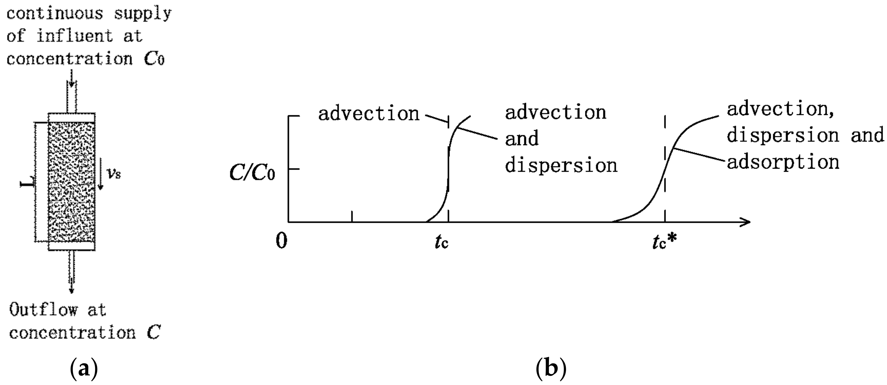
The mechanisms of pollutant migration include advection, hydrodynamic dispersion (including molecular diffusion and mechanical dispersion), and adsorption. The parameter representing advection is the pore flow velocity vs, the parameters representing hydrodynamic dispersion are the effective molecular diffusion coefficient Dd* (bending factor τ) and the diffusivity α, and the parameters representing the adsorption action are the retardation factor Rd and the nonlinear adsorption parameters. The flow velocity determines the appearance of the pollution front, the hydrodynamic dispersion parameter determines the width of the pollution front, and the adsorption has a retardation effect on migration, which delays the appearance of the pollution front. Figure 1 shows the breakthrough curves with a continuous source C0 at the top of the soil column. As shown in Figure 1, when only advection exists, the pollution front is pushed vertically like a piston; this is called piston flow, and the occurrence time is tc = L/vs, where L is the length of the column and vs is the seepage velocity. When there is both advection and hydrodynamic dispersion, the pollution front is a curve, and when there is also adsorption, the occurrence time of the pollution front is pushed backward, tc* = tc/Rd. Whether the hysteresis phenomenon caused by adsorption with different adsorption models is the same has not been discussed.
The one-dimensional transient solute transport through homogeneous soil can be described as
where Dh is coefficient of hydrodynamic dispersion, Dh = Dd* + Dm, Dd* = τDd, Dm = αvs, where Dd is free diffusion coefficient, Dm is mechanical dispersion. Rd = 1 when it is nonabsorbable, Rd is a constant greater than 1 under linear adsorption, and Rd is a function of pore water concentration under nonlinear adsorption, with its value changing with pore water concentration.
According to the adsorption model, a relationship between the total concentration in the soil and the pore water concentration can be established. The relationships for all three adsorption isotherms have been derived. The linear isotherm is the straight type, the Langmuir isotherm is the upper convex type, and the Freundlich isotherm (taking nf greater than 1) represents the lower concave type.
- (1)
- Linear isotherm (straight type).
The linear isotherm is expressed mathematically as
where Cs is the mass of contaminants adsorbed per unit dry mass of soil, Kd is the distribution coefficient, and Cw is the pore water concentration.
The corresponding retardation factor expression is:
where ρd is dry density, Kd is distribution coefficient, n is porosity.
According to the mass balance, the total concentration of pollutants Csto can be expressed as
In saturated soil, Sr = 1, so
Substituting Equation (5) into Equation (1), the governing equation for the mass concentration of pollutants in the soil can be obtained as follows:
Therefore, the analytical solution of the total concentration in the soil is equal to the analytical solution of the pore water multiplied by . Furthermore, the analytical solution can be used to fit the total concentration profile.
- (2)
- Langmuir sorption isotherm as upper convex type.
- (3)
- Freundlich sorption isotherm as lower concave type.
For a nonlinear sorption isotherm, because Csto and Cw are not simple linear relationships, it is impossible to obtain an analytical solution for the total concentration; however, the numerical method can be used to simulate Csto.
3. Scheme for Analyses and Discussion of Results
In this paper, the transport of pollutants considering a linear isotherm was analyzed based on the analytical solution, and the transport of pollutants considering nonlinear isotherms was analyzed by the finite difference method. Firstly, the pore water concentration Cw was calculated, and then the Csto profile was obtained based on the relationship between Cw and Csto. For the one-dimensional transport problem, the expressions for the pore water concentration Cw and the effluent concentration Ce adopted the boundary combination recommended by Zeng et al. [18]: the boundary combination of a continuous inlet flux and an infinite far-zero gradient of the outflow was used to simulate the pore water concentration Cw profile, and the boundary combination of a continuous inlet concentration and an infinite far-zero gradient of the outflow was used to analyze the effluent concentration Ce curve.
According to the compacted clay liner parameters given in the specification [34] and the relevant parameters reported in the literature [35,36], the main basic calculation parameters are shown in Table 1. The adsorption parameters are presented in the following sections.
3.1. Analysis of Influencing Factors of Advection–Dispersion Model for Linear Isotherm
According to the expressions for the pore water concentration Cw and effluent concentration Ce recommended by Zeng et al. [18], the dimensionless expressions are shown in Equations (13) and (14).
where , , T is the number of pore volumes of the flow, and PL is the Peclet number of soil columns representing the relative effect of advection with respect to the dispersive/diffusive transport.
The effluent concentration can be calculated according to Equation (16). In addition, the expression for the effluent concentration can be simplified when TR = T/Rd is substituted into Equations (13) and (14). It is then found that the expressions in Equations (13) and (14) for adsorbing solutes and non-adsorbing solutes are exactly the same. Dimensionless parameters were used directly in the following discussion. Dry density, porosity, and water content were taken from Table 1.
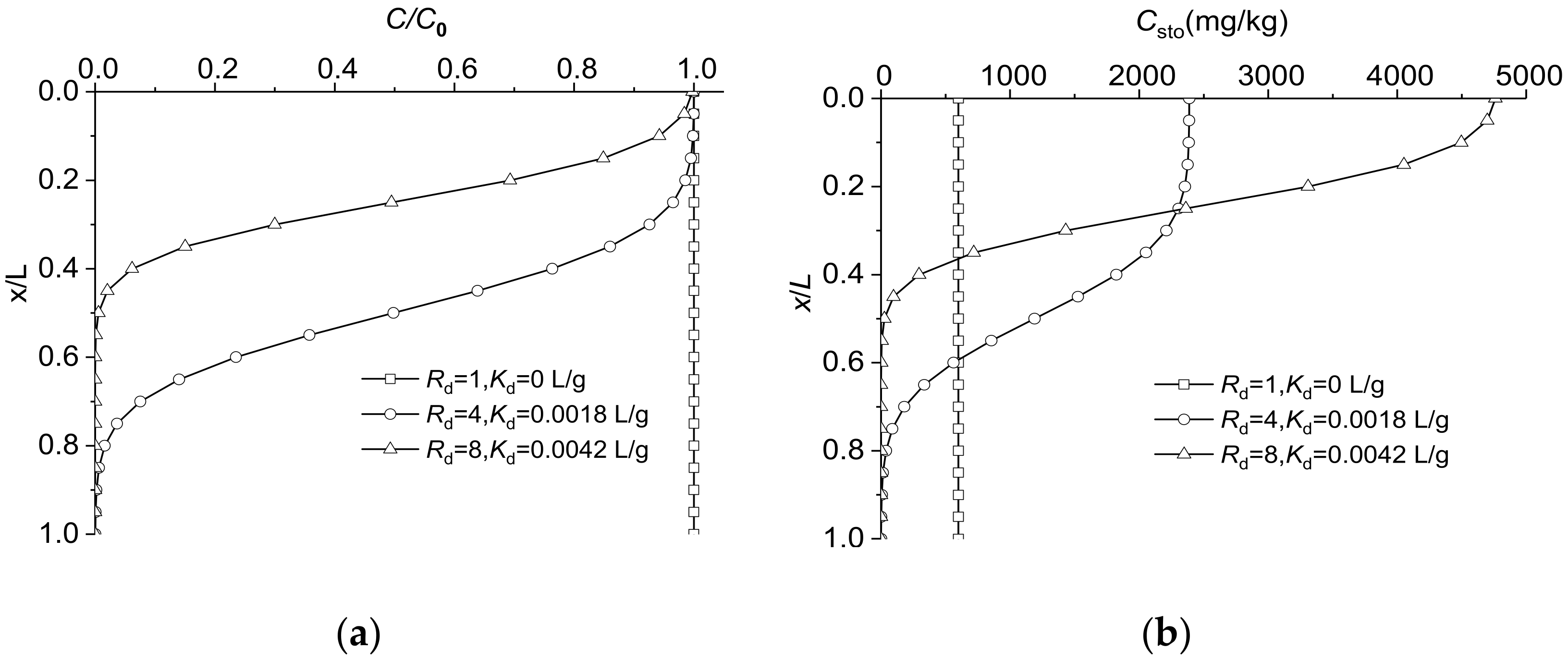
Figure 2a,b show the pore water and total concentration profiles in the clay liner corresponding to different retardation factors, respectively. Figure 2a shows that the larger the value of Kd (i.e., Rd), the shallower the contaminant front. Figure 2b shows that the larger the value of Kd (i.e., Rd), the shallower the total concentration profile curve in the soil and the bigger the peak value at the top.
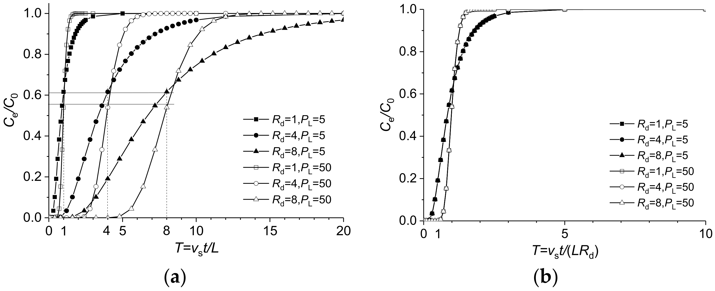
Figure 3 shows the breakthrough curves in terms of dimensionless parameters. As shown in Figure 3a, when T is taken as the abscissa, the greater the value of Kd, the later the effluent front appears and the wider the contaminant front in shape. When PL is the same, the concentration values corresponding to T = Rd on the breakthrough curves for different Kd values are equal: the greater the PL = vsL/Dh corresponding to the same Kd, the narrower the contaminant front. This is because a greater PL leads to a stronger advection effect; thus, its front is narrower. As shown in Figure 3b, when the abscissa is TR = vst/(LRd), the outflow concentration curves for different Rd values coincide, indicating that the effect of Rd on advection and dispersion is as shown in the control equation, that is, both vs and Dh are 1/Rd of the past, so that the effect of Rd on advection and dispersion migration is a linear superposition.
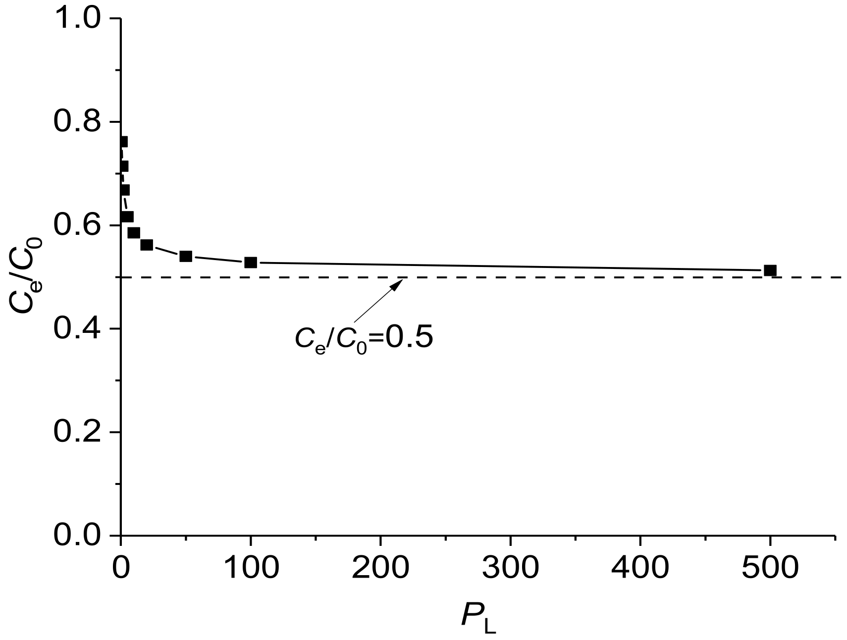
Figure 4 shows the relative outflow concentration values for different values of PL at T = Rd. When T = Rd, Ce/C0 is closer to 0.5. This is because the greater the PL, the greater the relative importance of advection and dispersion, and the sharper the concentration interface as a piston.
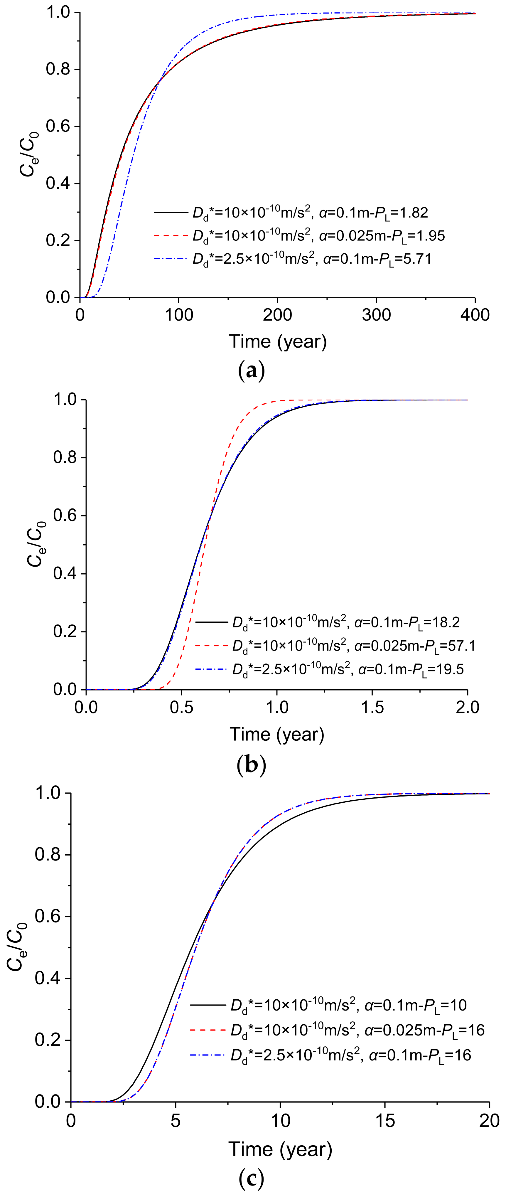
The effects of the two diffusion parameters Dd*(τ) and α are compared separately below. Figure 5a–c show the corresponding outflow curves with a 4-fold change of Dd* and α with three values of vs (vs = 1 × 10⁻⁹ m/s, 1 × 10⁻⁷ m/s, and 1 × 10⁻⁸ m/s), respectively, with a barrier thickness of 2 m. The values of Dd* and α are shown in the legends. As shown in Figure 5, when vs = 1 × 10⁻⁹ m/s, the effect of a 4-fold change in Dd* on the outflow curve was significantly greater than that of a 4-fold change in α. When vs = 1 × 10⁻⁷ m/s, the effect of a 4-fold change in α on the outflow curve was significantly greater than that of a 4-fold change in Dd*. When vs = 1 × 10⁻⁸ m/s, the outflow curves corresponding to 4-fold changes in Dd* and α coincided, that is, the effect was the same. According to the dimensionless parameters , the effects of Dd* and α are manifested in the change of PL, so that outflow curves with the same PL coincide. The smaller the flow rate, the greater the effect of Dd*, and conversely for the effect of α.
3.2. Analysis of Influencing Factors of Advection–Dispersion Model for Lower Concave Type
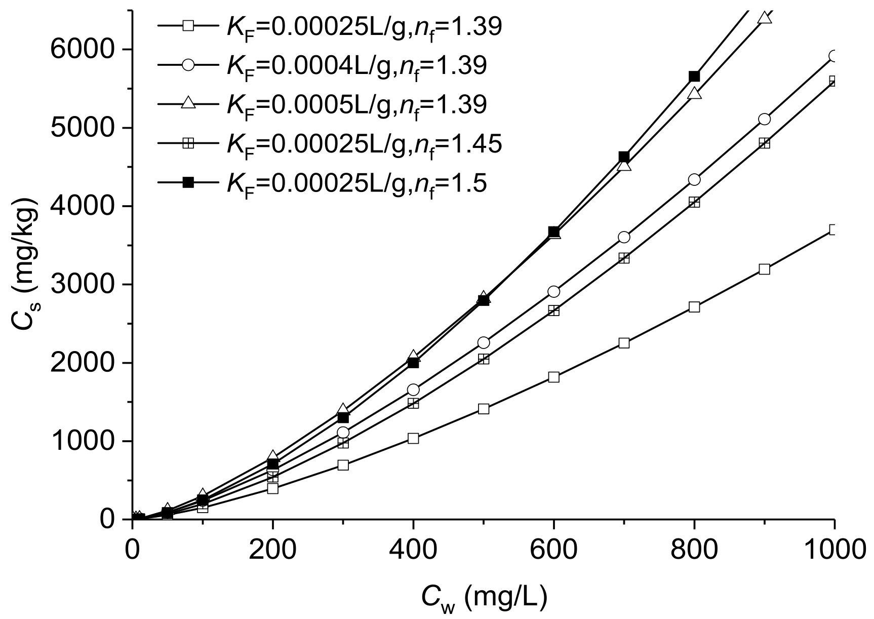
The Freundlich model has two parameters: KF and nf. The effects of the two parameters were compared separately, and in this section, C0 is assumed to be 1000 mg/L. The values of KF and nf used in the analysis are given in Table 2. All values of nf were greater than 1, so the isotherm is a lower concave curve. The corresponding adsorption isotherms are shown in Figure 6. When the effects of different source concentrations were compared, three source concentrations (1000 mg/L, 100 mg/L, and 10 mg/L) were considered, with KF and nf adsorption parameters taken from F1 in Table 2.
3.2.1. Effect of KF and nf
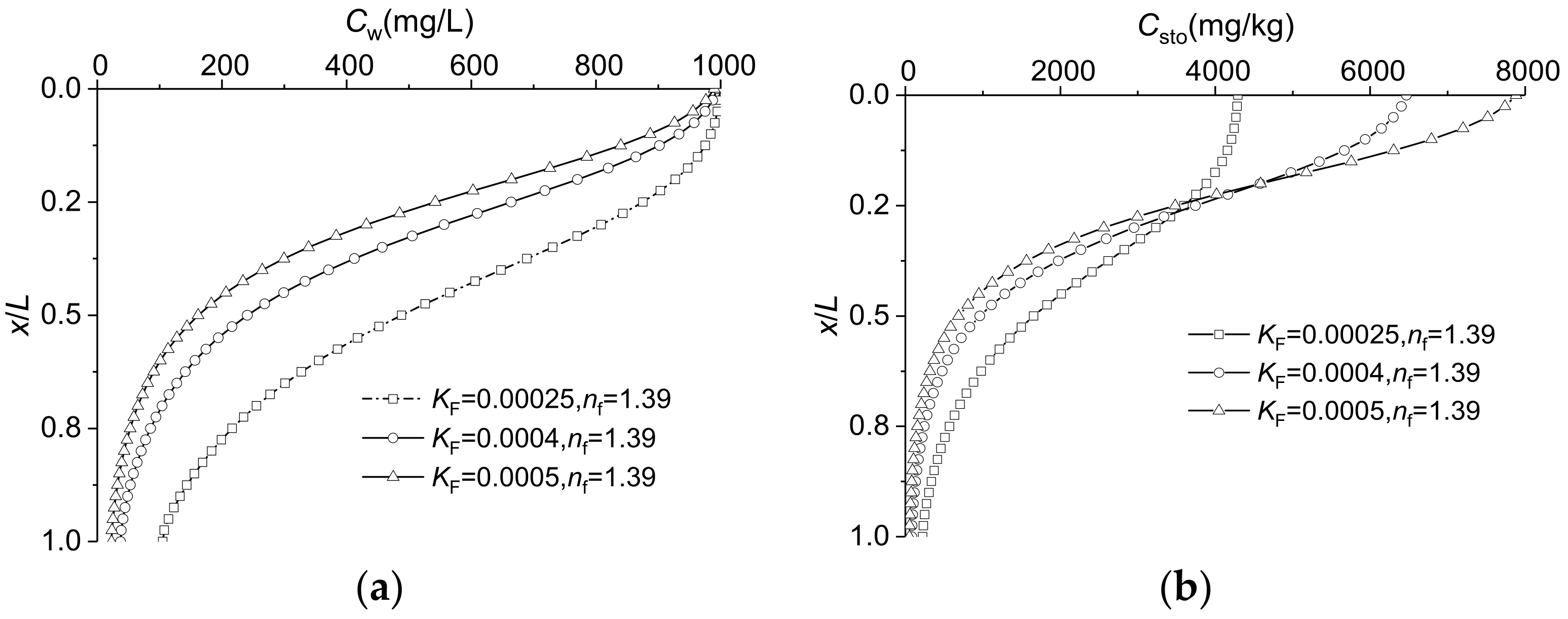
Figure 7a,b show the pore water concentration profiles and the total concentration profiles in soil with different values of KF at t = 24 h. As shown in Figure 7a, the larger the value KF, (i.e., the higher the isotherm), the greater the adsorption and the shallower the pore water concentration front. As shown in Figure 7b, the larger the value of KF, the shallower the total concentration profile curve in the soil and the greater the maximum value at the top.
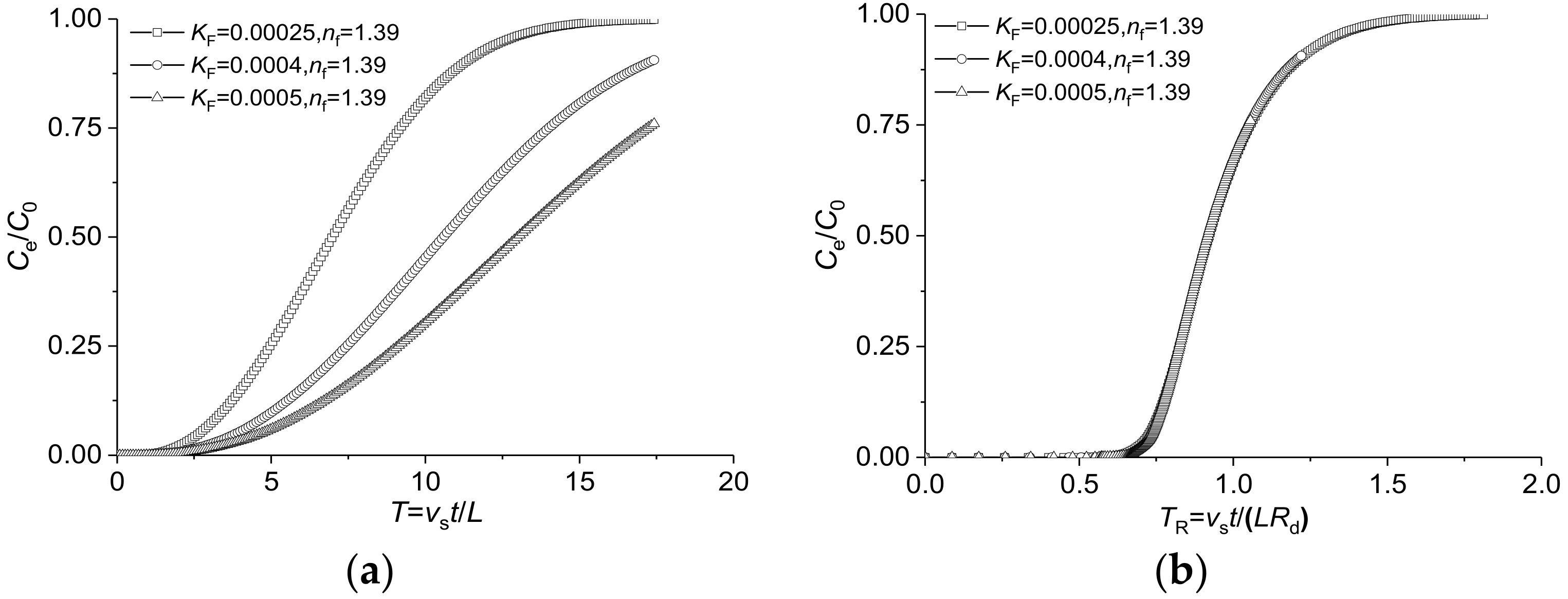
Figure 8a,b show the outflow concentration curves with T = vst/L as the abscissa and the outflow curves with TR = vst/(LRd) as the x-axis, respectively. The outflow curves with TR as the abscissa were obtained by substituting the Rd value calculated from Equation (13) into the outflow curve with T as the abscissa. As shown in Figure 8a, the larger the value of KF, the later the outflow curve appears. As shown in Figure 8b, when TR is taken as the abscissa, all the outflow curves basically coincide.
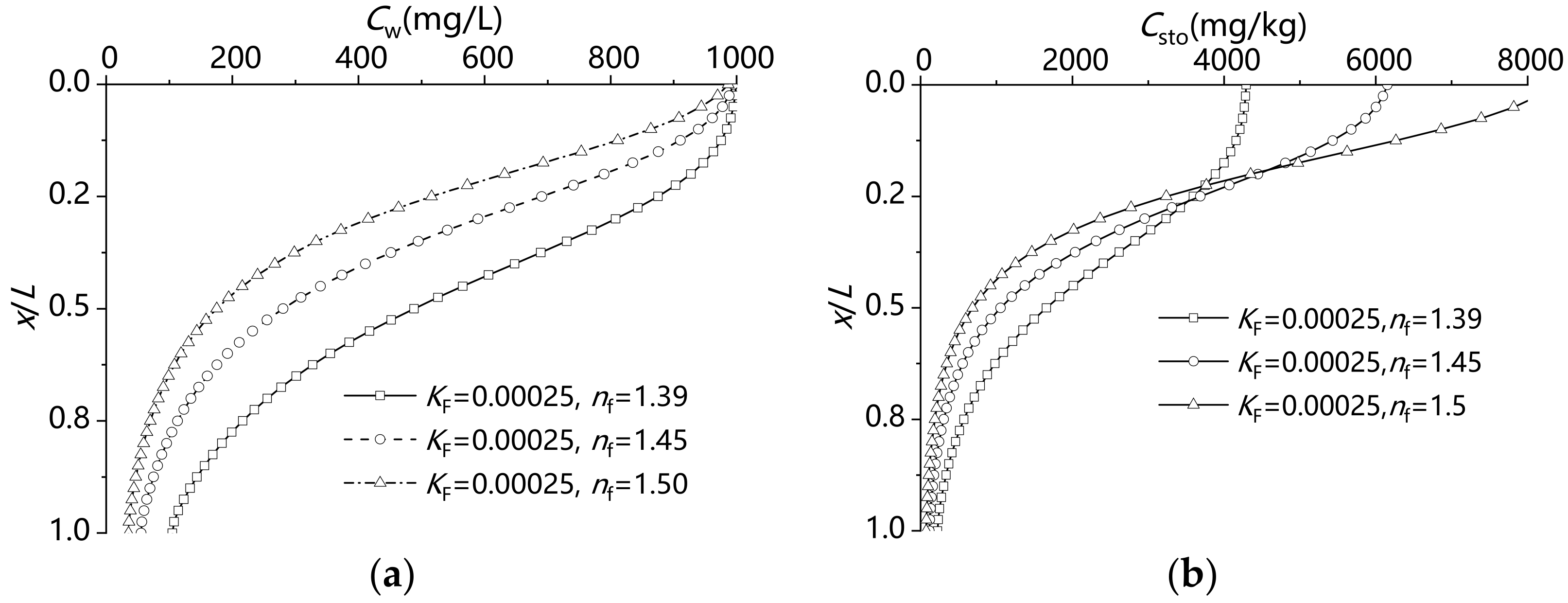
Figure 9a,b show the pore water profiles and the total concentration profiles in soil with different values of nf at t = 24 h. As shown in Figure 9a, the larger the value of nf, (i.e., the higher the isotherm), the greater the adsorption and the shallower the pore water concentration front. As shown in Figure 9b, the larger the value of nf, the shallower the total concentration profile curve in the soil and the greater the maximum value at the top.
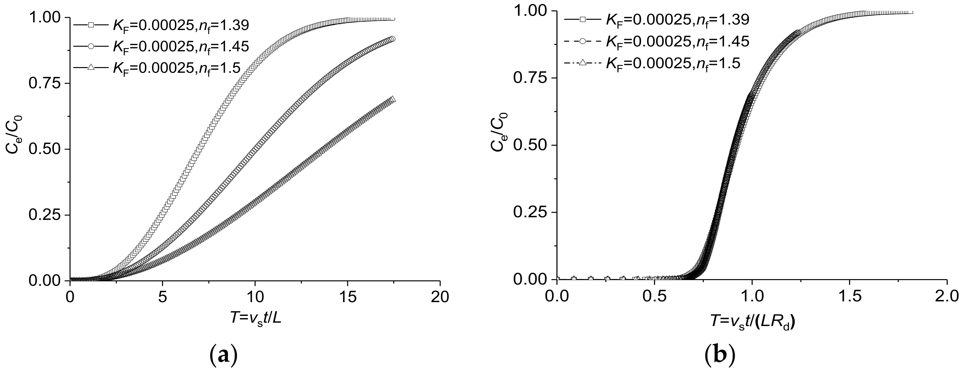
Figure 10a,b show the outflow concentration curves with T = vst/L as the abscissa and the outflow curves with TR = vst/(LRd) as the x-axis, respectively. As shown in Figure 10a, the larger the value of nf, the later the outflow curve appears. As shown in Figure 10b, when TR is taken as the abscissa, all the outflow curves basically coincide.
3.2.2. Effect of Source Concentration
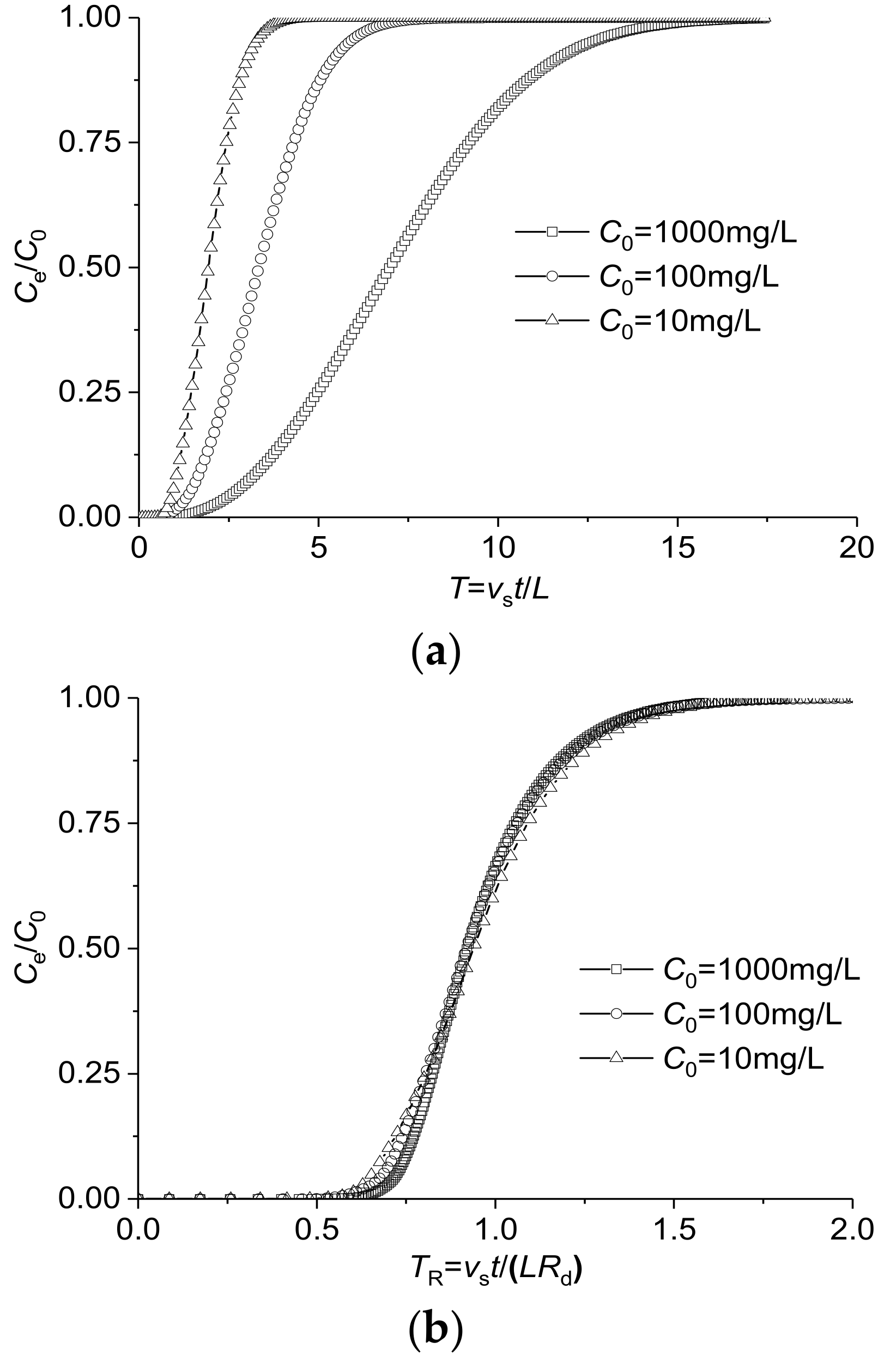
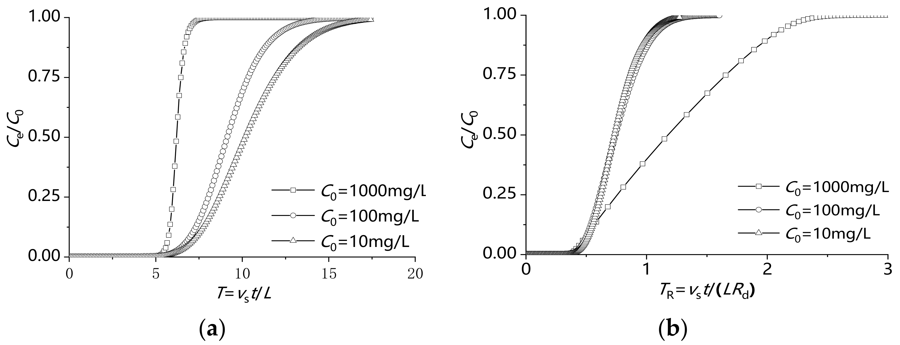
Figure 11a,b show the outflow concentration curves with T = vst/L as the abscissa and the outflow curves with TR = vst/(LRd) as the x-axis, respectively. As shown in Figure 11a, when T is taken as the abscissa, the smaller the source concentration, the earlier the outflow curve appears. As shown in Figure 11b, when TR is taken as the abscissa, the outflow curves corresponding to different source concentrations are relatively close, but do not coincide, which indicates that the effect of C0 on advection and dispersion migration in the nonlinear adsorption model is nonlinear.
3.3. Analysis of Influencing Factors of Advection–Dispersion Model for Upper Convex Type
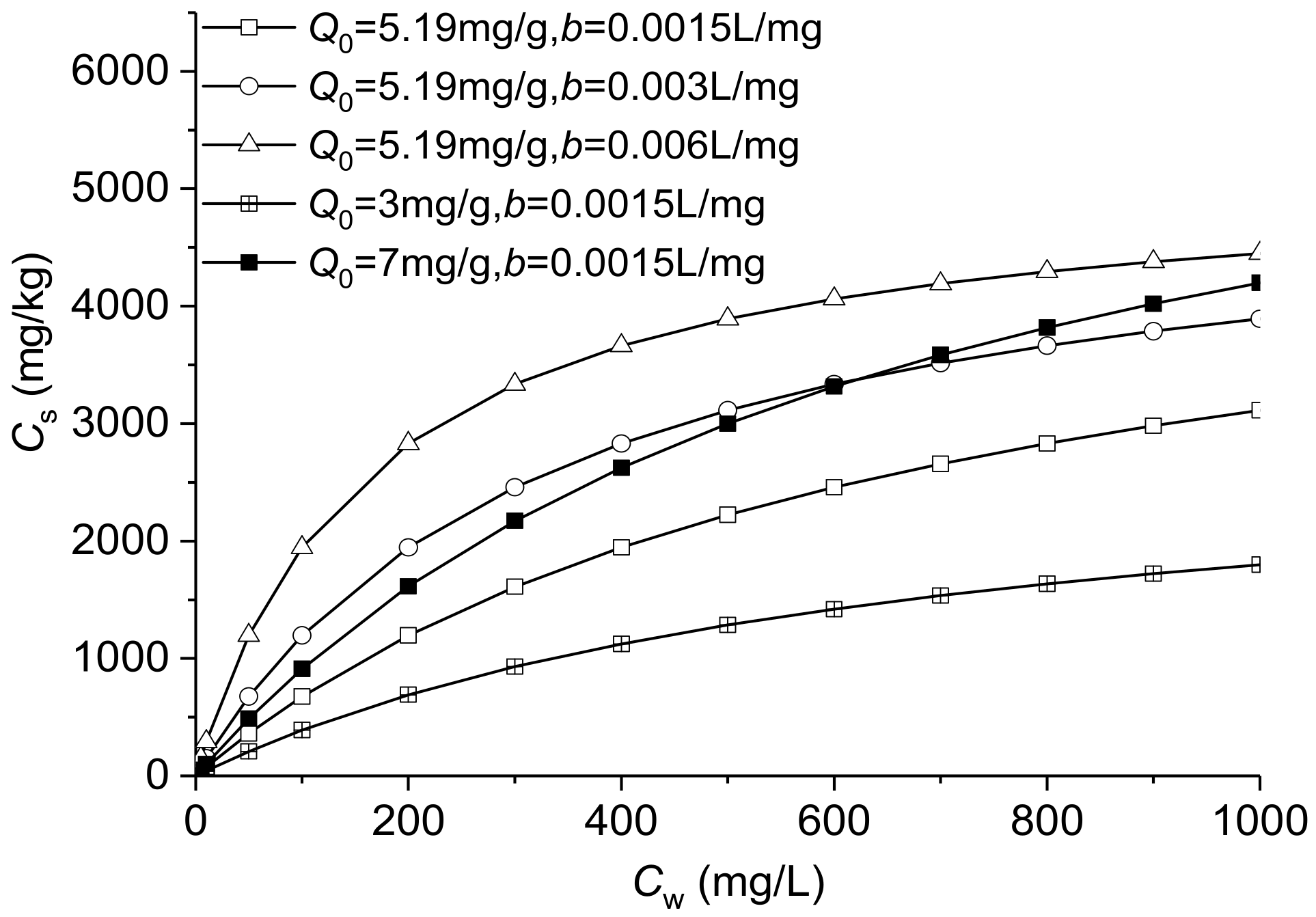
The Langmuir model has two parameters: Q0 and b. The effects of these two adsorption parameters were compared separately in the analysis, and in this section, C0 is assumed to be 1000 mg/L. The values of Q0 and b used in the analysis are given in Table 3, and the corresponding adsorption isotherms are shown in Figure 12. The effects of different source concentrations for the same adsorption parameter were compared. Three source concentrations (1000 mg/L, 100 mg/L, and 10 mg/L) were considered, with the adsorption parameters Q0 and b taken from L1 in Table 3.
3.3.1. Effect of Q0 and b
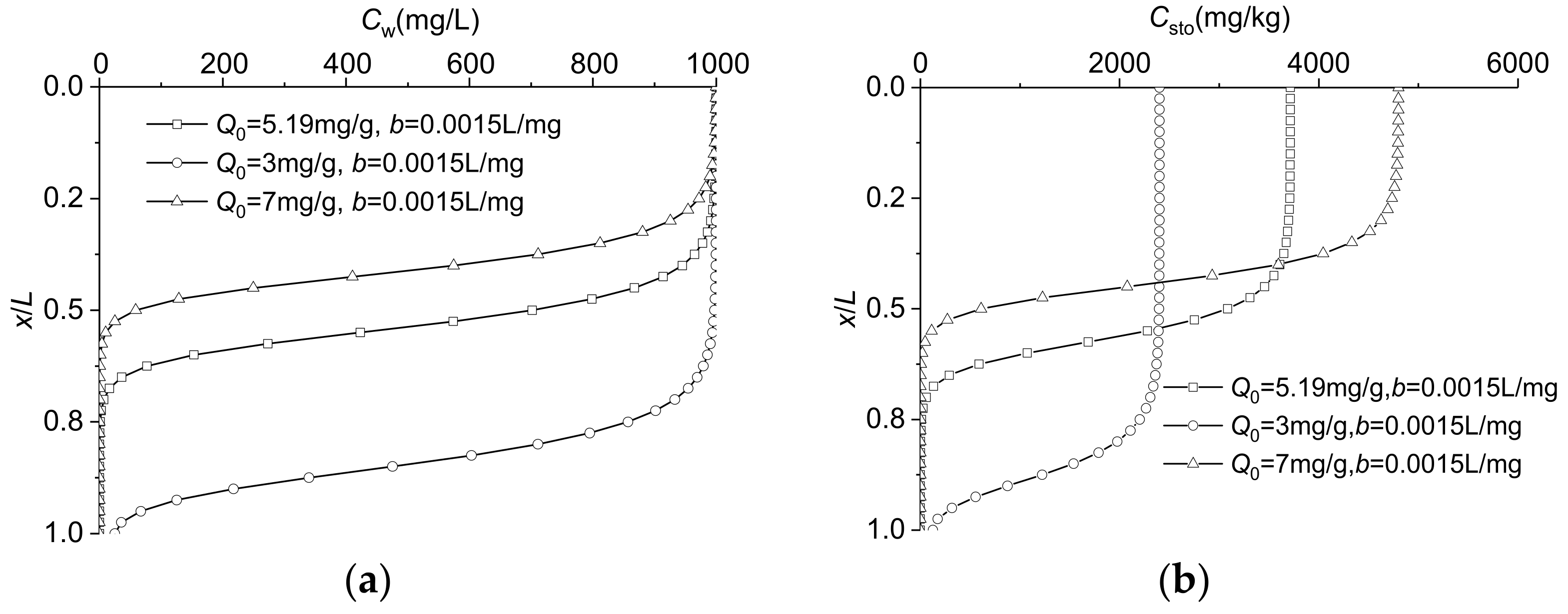
Figure 13a,b show the pore water concentration profiles and the total concentration profiles in soil with different values of Q0 at t = 24 h. As shown in Figure 13a, the larger the value of Q0 (i.e., the higher the isotherm), the higher the isothermal adsorption curve, the greater the adsorption, and the shallower the pore water concentration front. As shown in Figure 13b, the larger the value of Q0, the shallower the total concentration profile curve in the soil and the greater the maximum value at the top.
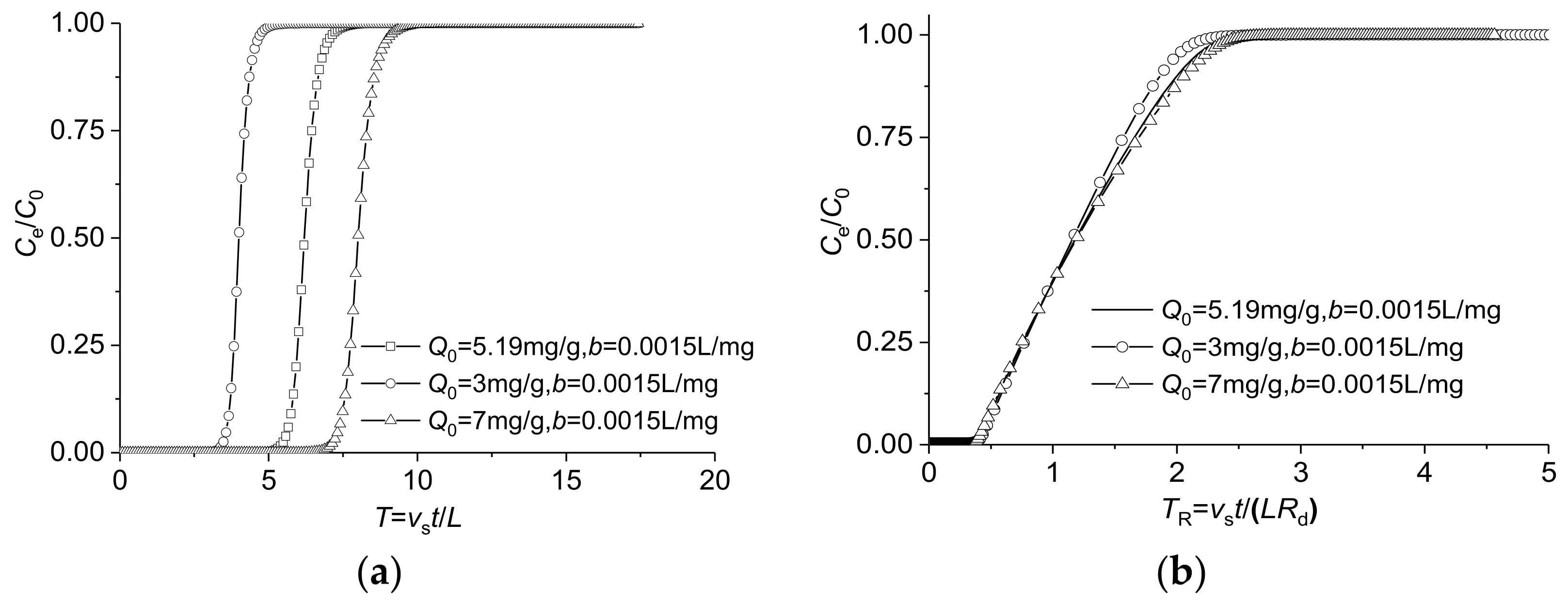
Figure 14a,b show the outflow concentration curves with T as the abscissa and the outflow curves with TR as the x-axis, respectively. As shown in Figure 14a, the larger the value of Q0, the higher the isothermal adsorption curve, the later the outflow curve appears, and the flatter the concentration front. As shown in Figure 14b, when TR is taken as the abscissa, all the corresponding flow curves are very close.
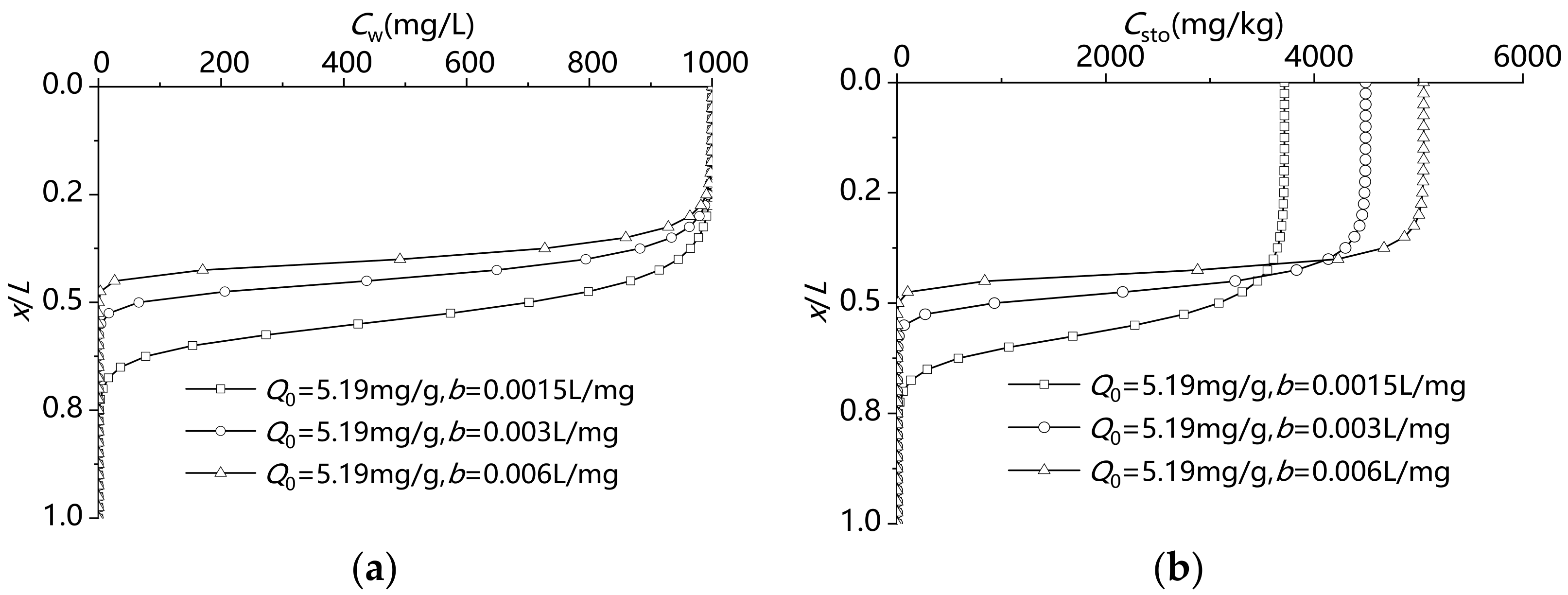
Figure 15a,b show the pore water profiles and the total concentration profiles in soil with different values of b at t = 24 h. As shown in Figure 15a, the larger the value of b, (i.e., the higher the isotherm), the greater the adsorption and the shallower the pore water concentration front. As shown in Figure 15b, the larger the value of b, the shallower the total concentration profile curve in the soil and the greater the maximum value at the top.
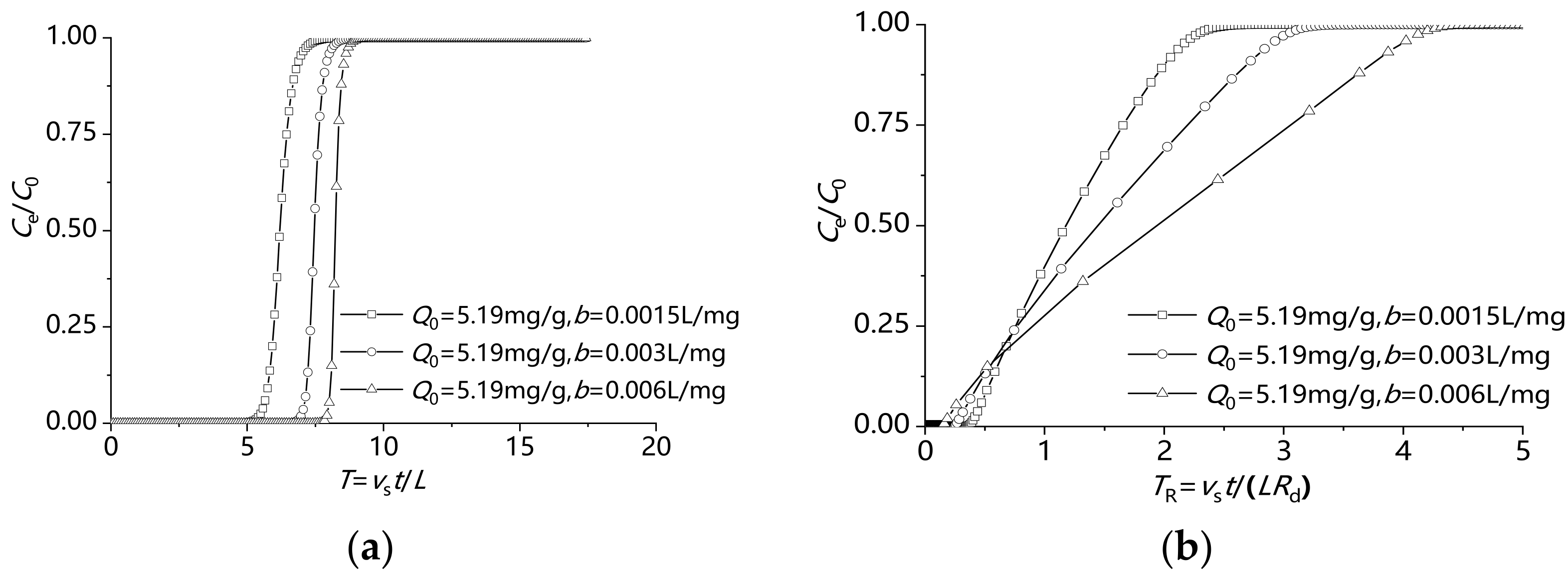
Figure 16a,b show the outflow concentration curves with T as the abscissa and the outflow curves with TR as the x-axis, respectively. As shown in Figure 16a, the larger the value of b, the later the outflow curve appears. As shown in Figure 16b, when TR is taken as the abscissa, all the outflow curves of the Langmuir model are quite different, and there is an intersection point.
3.3.2. Effect of Source Concentration
Figure 17a,b show the outflow concentration curves with T as the abscissa and the outflow curves with TR as the x-axis, respectively. As shown in Figure 17a, when T is taken as the abscissa, the smaller the source concentration, the later the outflow curve appears. As shown in Figure 17b, when TR is taken as the abscissa, the outflow curves corresponding to the different source concentrations do not coincide and are quite different.
3.4. Effect of Different Types of Sorption Isotherms with the Same Maximum Adsorption Capacity
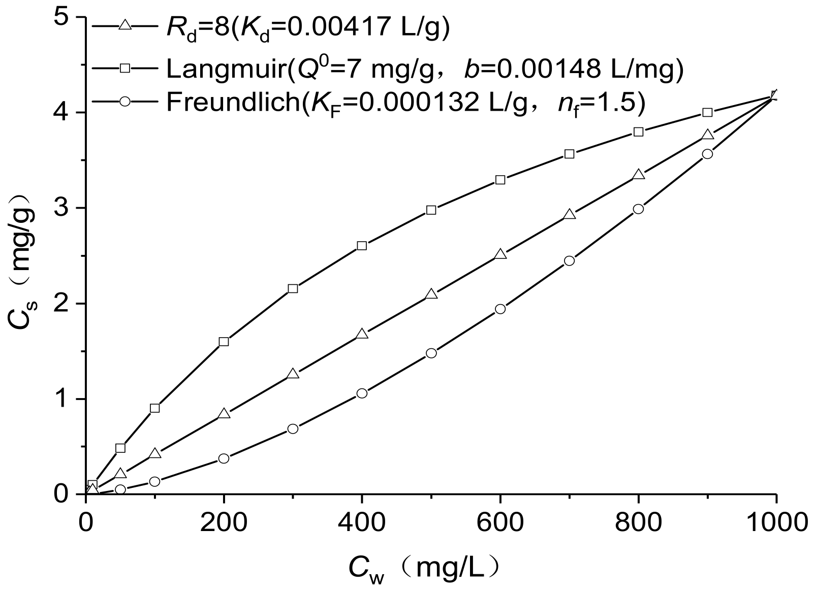
Three types of isotherms: upper convex, linear, and lower concave, with the same maximum adsorption capacity, are compared below, represented by the Langmuir model, the linear model, and the Freundlich model, respectively. The specific adsorption parameters are shown in Figure 18. The other parameters used in the calculation are given in Table 1.
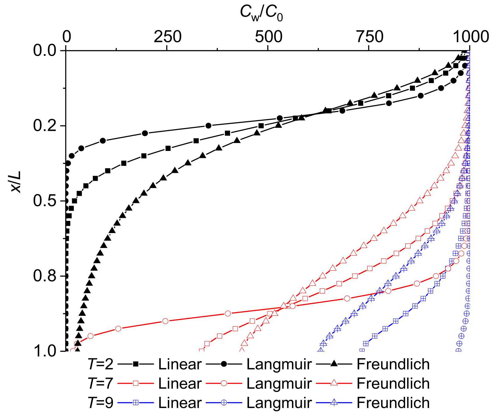
Figure 19 shows the pore water concentration profiles. As shown in Figure 19, there is a common intersection point in the three concentration profiles: above the intersection point, the concentration front of the upper convex (Langmuir model) is the deepest, and the concentration front of the lower concave (Freundlich model) is the shallowest; below the intersection point, the concentration front of the upper convex (Langmuir model) is the shallowest, and the concentration front of the lower concave (Freundlich model) is the deepest. With increasing time, the intersection-point position on the profile gradually moves downward. As a whole, the concentration front of the upper convex (Langmuir model) is the narrowest, followed by the linear model, and the lower concave (Freundlich model) is the widest.
The slopes (partition coefficients) for each isotherm are as follows: in the low pore water concentration segment, the upper convex type (Langmuir model) > linear model > lower concave type (Freundlich model), that is, the upper convex adsorption rate is largest and the lower concave adsorption rate is smallest; in the high pore water concentration segment, the upper convex type (Langmuir model) < linear model < lower concave type (Freundlich model), that is, the upper convex adsorption rate is smallest and the lower concave adsorption rate is largest. Therefore, there is an intersection point in the pore water concentration front of different models.
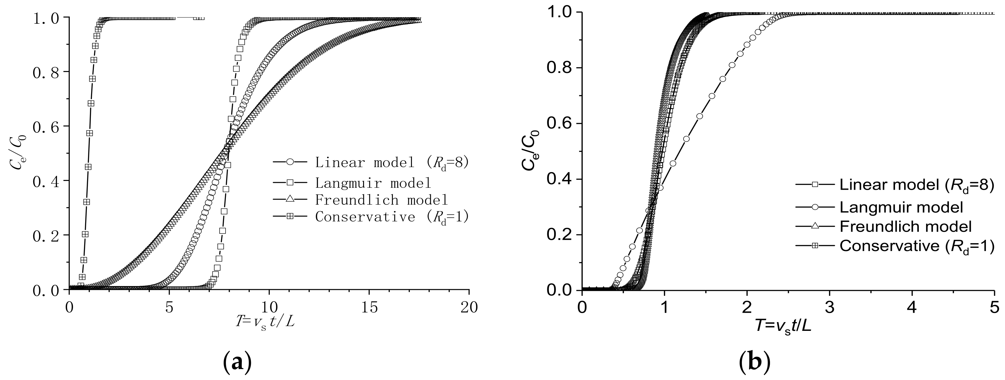
Figure 20a,b show the outflow concentration curves with T as the abscissa and the outflow curves with TR as the x-axis, respectively. As shown in Figure 20a, when T is taken as the abscissa, there is a common intersection point in the three curves, and before the intersection point, the order of the outflow concentration is lower concave (Freundlich model) > linear > upper convex (Langmuir model), with the opposite after the intersection point. The lower concave (Freundlich model) outflow concentration appeared first, followed by the linear model, with the upper convex (Langmuir model) appearing latest. The upper convex (Langmuir model) reached equilibrium first, the linear model in the middle, and the lower concave (Freundlich model) latest. This is consistent with the distribution of pore water concentrations shown in Figure 19. As shown in Figure 20b, when TR is taken as the abscissa, the outflow curves of different isotherms do not coincide and there are intersections.
Comparing Figure 20a with Figure 3a, it can be seen that compared with the linear model, the Langmuir model corresponds to a narrower concentration front, which is similar to the effect of a smaller Dh (i.e., PL), and the Freundlich model corresponds to a wider concentration front, which is similar to the effect of a larger Dh (i.e., PL), that is, the nonlinear adsorption model has a similar effect on the shape of the outflow curve as changing Dh. Therefore, the nonlinear adsorption behavior may be mistakenly defined as linear adsorption by fitting the diffusion parameters and adsorption parameters at the same time. For this reason, univariate analysis is recommended in the analysis of the test results. That is, migration parameters should be fitted one by one in the study.
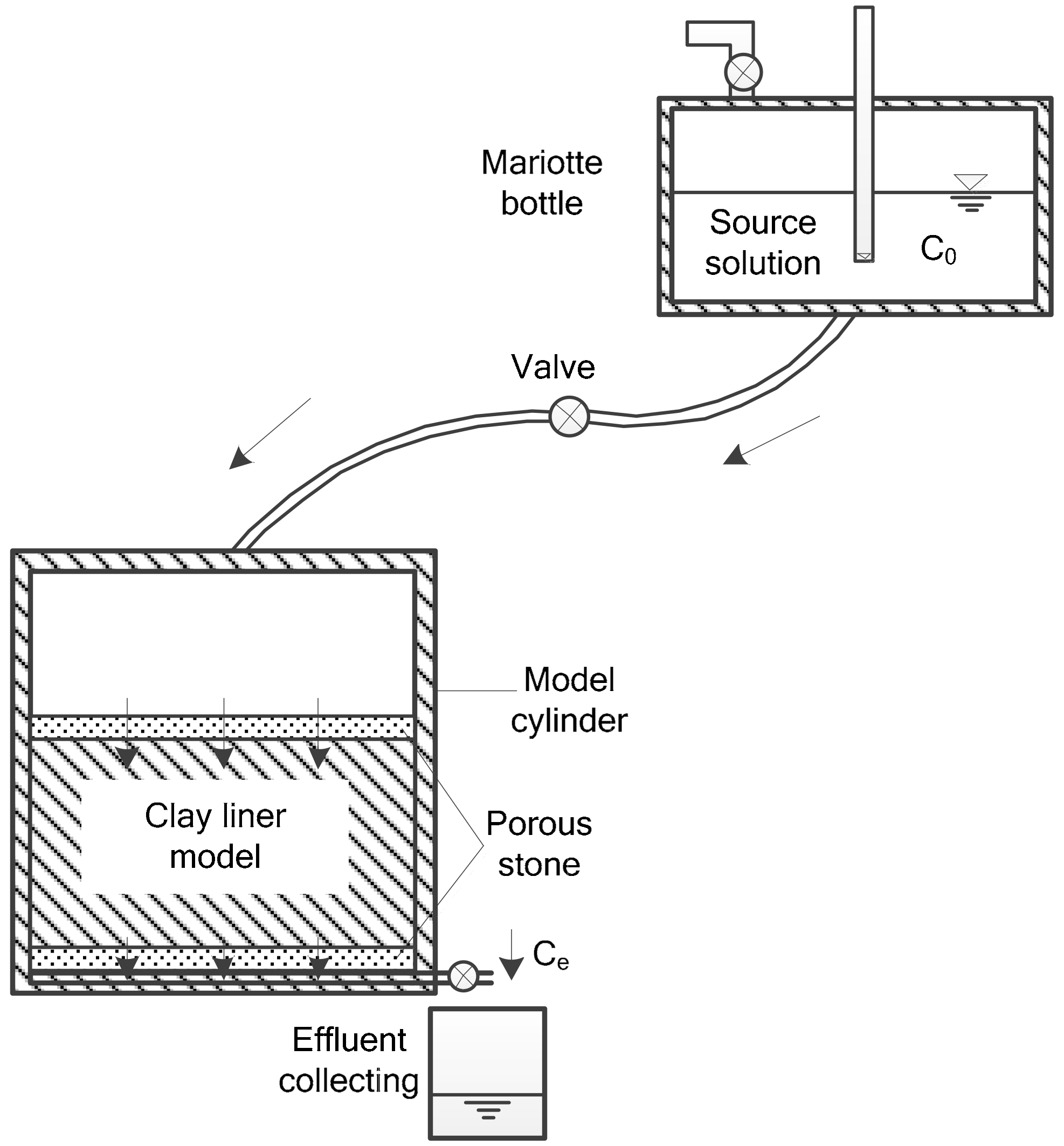
3.5. Column Test with Pb2+
In order to illustrate the different types of isotherms, a breakthrough column test with a source solution of Pb(II) was carried out. Kaolin clay slurry was consolidated for preparing the clay liner model in a model cylinder. The physical parameters of kaolin are given in Table 4.
As shown in Figure 21, after completion of the consolidation, the model cylinder was connected to a modified Mariotte bottle which was used to contain the designed hydraulic head. The source concentration C0 of Pb(II) was kept constant at 892.3 mg/L. The test was started by turning on the two control valves for inflow and outflow. The effluent from the bottom of the model cylinder was collected at a series of different times. The effluent concentration was measured using an atomic absorption spectrophotometer (TAS-990).
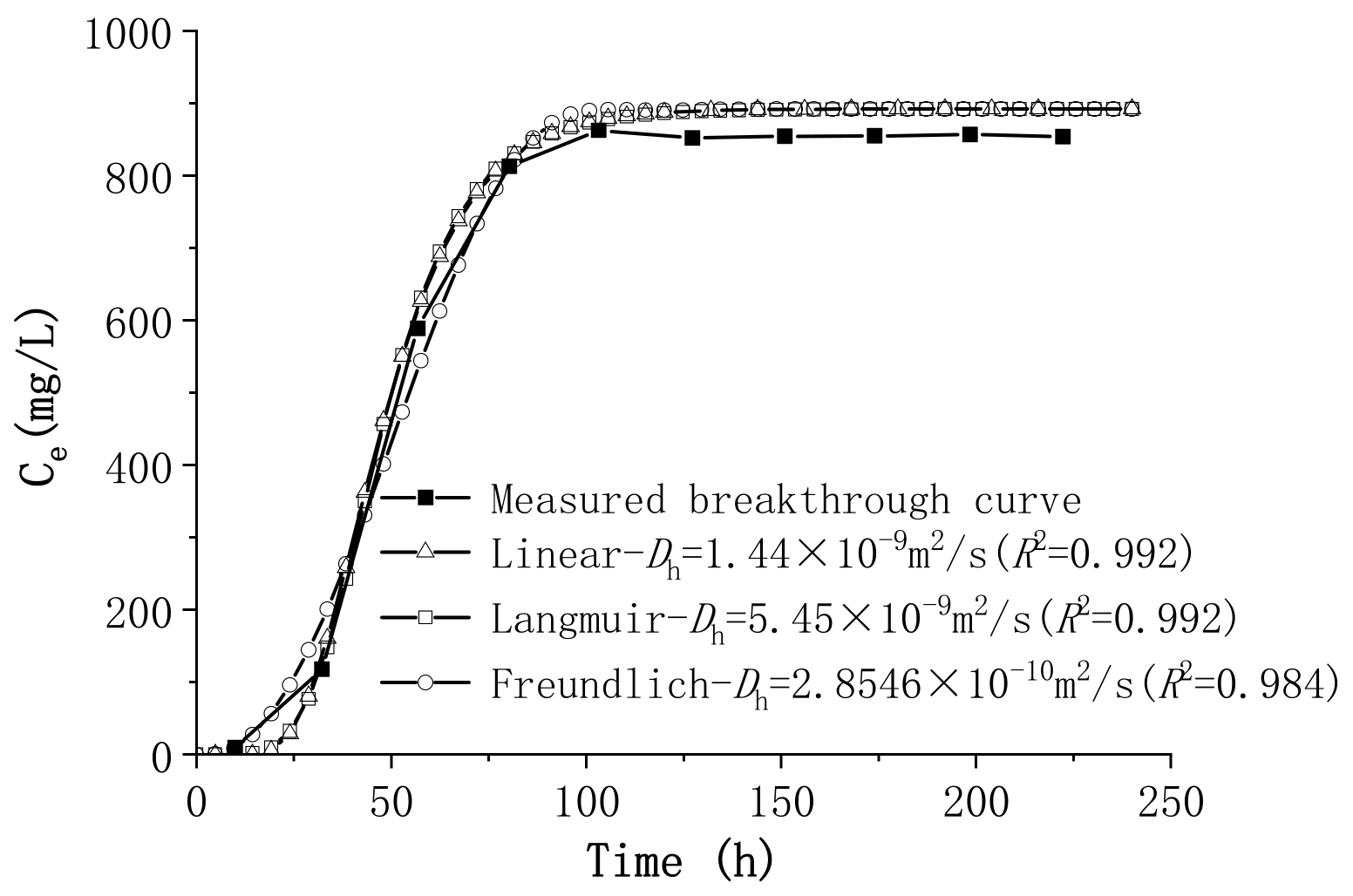
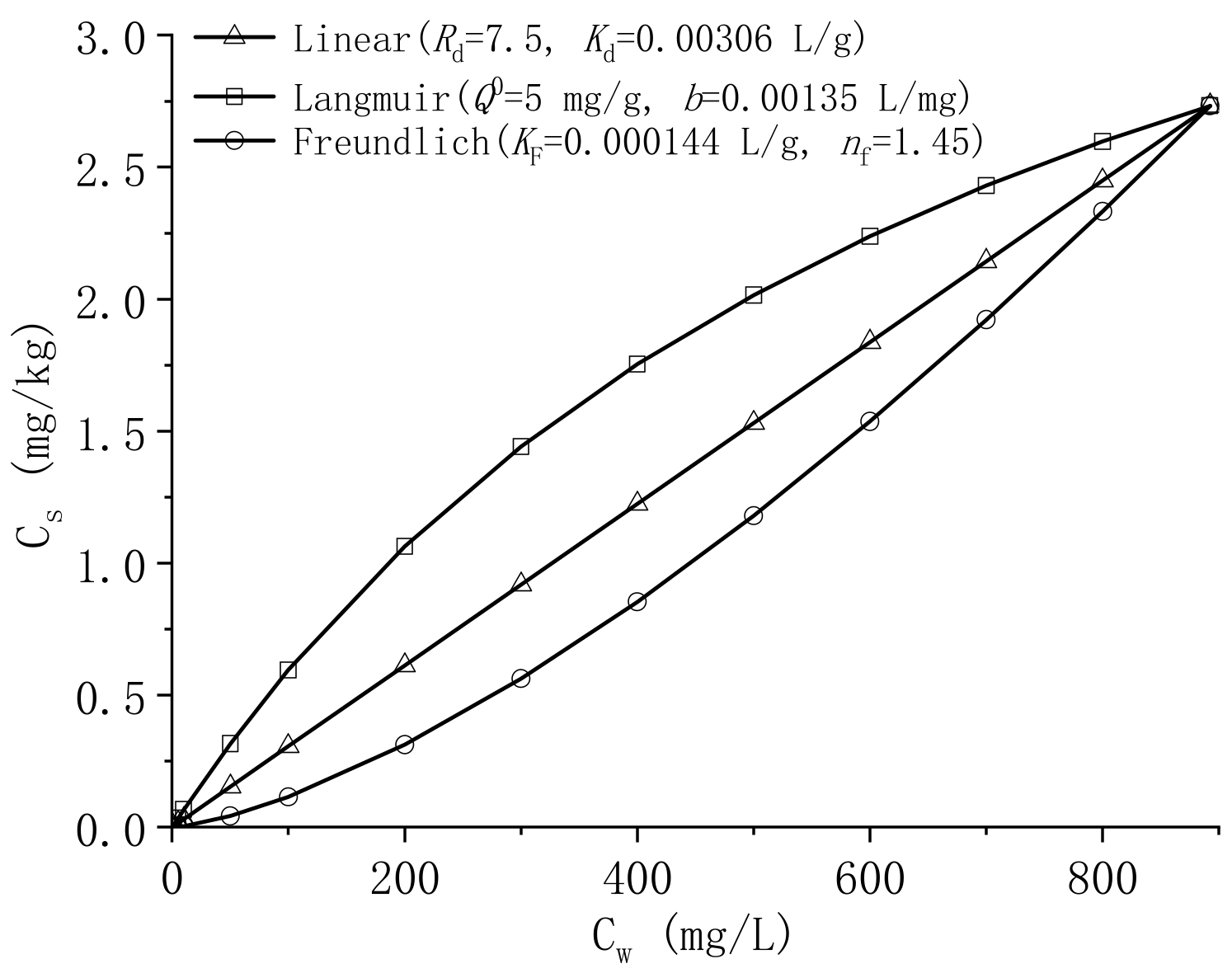
Table 5 shows the parameters of the column test. The height of the column was 21.9 mm, and the hydraulic head difference was 16m, corresponding to an advection velocity of 9.01 × 10⁻⁷ m/s. Figure 22 shows a comparison of the measured breakthrough curve and the fitting breakthrough curves. The best-fit value of Rd was 7.5 as shown in Figure 22. Meanwhile, the Langmuir isotherm and the Freundlich isotherm with the same maximum adsorption capacity were compared, as shown in Figure 23. As shown in Figure 22, the Langmuir isotherm was able to fit the measured curve very well (determination coefficient R2 = 0.992). However, the best-fit value of Dh was 5.45 × 10⁻⁹ m2/s, which was much larger than a reasonable value. The Freundlich isotherm fit the measured curve somewhat less well (R2 = 0.984) than the other two isotherms, and the fitted value of Dh was 2.8546 × 10⁻¹⁰ m2/s, which was much smaller than a reasonable value. Hence, it was verified that the nonlinear adsorption model had a similar effect on the shape of the outflow curve as changing the value of Dh.
4. Conclusions
The concentration profiles and outflow curves of the 2 m thick compacted clay liner (CCL) given in the specification were calculated, considering three different sorption isotherms (upper convex, linear, and lower concave). The effects of transport parameters, sorption isotherms, and source concentrations on pollutant migration were analyzed. The results showed that the effect of source concentrations on pollutant migration was different for different adsorption models. Source concentration values had no effect on the migration of the linear adsorption model, but for the Langmuir model, migration was slow for small source concentrations, and for the Freundlich model, migration was slow for large source concentrations. Because the partition coefficient of the linear isothermal adsorption curve was constant and did not change with concentration, the upper convex (Langmuir model) isothermal adsorption curve had a larger partition coefficient at smaller concentrations, and the lower concave (Freundlich model) isothermal adsorption curve had a smaller partition coefficient at smaller concentrations. With a small partition coefficient, the adsorption was low and the concentration front was deep; conversely, the concentration front was shallow with a larger partition coefficient.
When the adsorption capacity corresponding to the source concentration was the same as in the linear model, the effect of the nonlinear adsorption model on the shape of the outflow curve was similar to the effect of a change in diffusion (Dh): the concentration front corresponding to the upper convex model was narrower, which was similar to the effect of Dh (i.e., PL) reduction, and the concentration front corresponding to the lower concave model was wider, which was similar to the effect of an increased Dh (i.e., PL)). These results were verified using a column test. Therefore, the nonlinear adsorption behavior may be mistakenly defined as linear adsorption by fitting the diffusion parameters and adsorption parameters at the same time. For this reason, univariate analysis was recommended for analysis of the results. In other words, the diffusion and adsorption parameters should be fitted separately in the study.
When the flow rate was small, the effect of Dd* on the curve was large, and the effect of α was small, while there were opposite effects when the flow rate was large. The adsorption had a significant effect on the outflow curve, so it is very important to obtain the correct adsorption parameters for the prediction of the CCL’s performance.
Author Contributions
Conceptualization, X.Z. and J.Y.; methodology, X.Z. and H.W.; software, H.W.; validation, X.Z. and Y.L.; formal analysis, X.Z. and H.W.; investigation, X.Z. and J.Y.; resources, X.Z.; data curation, J.Y.; writing—original draft preparation, X.Z. and H.W.; writing—review and editing, X.Z. and Y.L.; visualization, X.Z. and H.W.; supervision, H.W.; project administration, X.Z.; funding acquisition, X.Z and H.W. All authors have read and agreed to the published version of the manuscript.
Funding
This work was supported in part by the National Natural Science Foundation of China (Grant No. 41702329), in part by the Scientific Research Fund of Hunan Provincial Education Department (Grant No. 17B097), in part by Department of Natural Resources of Hunan Province (Grant No. 2020-15), in part by the Zhejiang Provincial Natural Science Foundation (No. LQ18E080001), and in part by the Ningbo City Science and Technology Project for Public Benefit (No. 2019C50014).
Institutional Review Board Statement
Not applicable.
Informed Consent Statement
Not applicable.
Data Availability Statement
The data presented in this study are available on request from the corresponding author.
Conflicts of Interest
The authors declare no conflict of interest.
References
- Brozni, D.; Mirna, P.; Rimac, V.; Marini, J. Sorption and leaching potential of organophosphorus insecticide dimethoate in Croatian agricultural soils. Chemosphere 2020, 273, 128563. [Google Scholar] [CrossRef]
- Sharma, P.K.; Sawant, V.A.; Shukla, S.; Khan, Z. Experimental and numerical simulation of contaminant transport through layered soil. Int. J. Geotech. Eng. 2014, 8, 345–351. [Google Scholar] [CrossRef]
- Zhu, F.; Liu, T.; Zhang, Z.; Liang, W. Remediation of hexavalent chromium in column by green synthesized nanoscale zero-valent iron/nickel: Factors, migration model and numerical simulation. Ecotoxicol. Environ. Saf. 2020, 207, 111572. [Google Scholar] [CrossRef] [PubMed]
- Shackelford, C.D.; Redmond, P.L. Solute breakthrough curves for processed kaolin at low flow rates. J. Geotech. Eng. 1995, 120, 17–32. [Google Scholar] [CrossRef]
- Kererat, C.; Sasanakul, I.; Soralump, S. Centrifuge Modeling of LNAPL Infiltration in Granular Soil with Containment. J. Geotech. Geoenvironmental Eng. 2013, 139, 892–902. [Google Scholar] [CrossRef] [Green Version]
- Nakajima, H.; Hirooka, A.; Takemura, J.; Mariño, M.A. Centrifuge modeling of one-dimensional subsurface contamination. JAWRA J. Am. Water Resour. Assoc. 1998, 34, 1415–1425. [Google Scholar] [CrossRef]
- Basford, J.; Goodings, D.J.; Torrents, A. Fate and transport of lead through soil at 1 g and in the centrifuge. In Physical Modelling in Geotechnics: ICPMG 02, Proceedings of the International Conference, St John’s, NL, Canada, 10–12 July 2002; Phillips, R., Guo, P.J., Popesu, R., Eds.; AA Balkema: Rotterdam, The Netherlands, 2002; pp. 379–383. [Google Scholar]
- Wang, L.; Huang, P.; Liu, S.; Shen, C.; Lu, Y. Analytical solutions for one-dimensional contaminant ion transport through electro-kinetic barriers. J. Hydrol. 2020, 597, 125756. [Google Scholar] [CrossRef]
- Lin, Y.C.; Yeh, H.D. A Simple Analytical Solution for Organic Contaminant Diffusion through a Geomembrane to Unsaturated Soil Liner: Considering the Sorption Effect and Robin-Type Boundary. J. Hydrol. 2020, 586, 124873. [Google Scholar] [CrossRef]
- Purkayastha, S.; Kumar, B. Analytical solution of the one-dimensional contaminant transport equation in groundwater with time-varying boundary conditions. ISH J. Hydraul. Eng. 2018, 26, 78–83. [Google Scholar] [CrossRef]
- Feng, S.-J.; Peng, M.-Q.; Chen, Z.-L.; Chen, H.-X. Transient analytical solution for one-dimensional transport of organic contaminants through GM/GCL/SL composite liner. Sci. Total. Environ. 2018, 650, 479–492. [Google Scholar] [CrossRef] [PubMed]
- Yu, C.; Wang, H.; Fang, D.; Ma, J.; Cai, X.; Yu, X. Semi-analytical solution to one-dimensional advective-dispersive-reactive transport equation using homotopy analysis method. J. Hydrol. 2018, 565, 422–428. [Google Scholar] [CrossRef]
- Xie, H.; Jiang, Y.; Zhang, C.; Feng, S. An analytical model for volatile organic compound transport through a composite liner consisting of a geomembrane, a GCL, and a soil liner. Environ. Sci. Pollut. Res. 2014, 22, 2824–2836. [Google Scholar] [CrossRef]
- Shackelford, C.D. Analytical Models for Cumulative Mass Column Testing. In Geoenvironment; ASCE: New York, NY, USA, 1995. [Google Scholar]
- Parlange, J.-Y.; Starr, J.L.; VAN Genuchten, M.T.; Barry, D.A.; Parker, J.C. Exit condition for miscible displacement experiments. Soil Sci. 1992, 153, 165–171. [Google Scholar] [CrossRef]
- Novakowski, K.S. An evaluation of boundary conditions for one-dimensional solute transport: 2. Column experiments. Water Resour. Res. 1992, 28, 2411–2423. [Google Scholar] [CrossRef]
- Schwartz, R.C.; McInnes, K.J.; Juo, A.S.R.; Wilding, L.P.; Reddell, D.L. Boundary effects on solute transport in finite soil columns. Water Resour. Res. 1999, 35, 671–681. [Google Scholar] [CrossRef]
- Zeng, X.; Zhan, L.T.; Chen, Y.M. Applicability of boundary conditions for analytical modelling of advection-dispersion transport in low-permeability clay column tests. Chin. J. Geotech. Eng. 2017, 39, 636–644. [Google Scholar]
- Groisman, L.; Rav-Acha, C.; Gerstl, Z.; Mingelgrin, U. Sorption of organic compounds of varying hydrophobicities from water and industrial wastewater by long- and short-chain orgnaoclays. Appl. Clay Sci. 2004, 24, 159–166. [Google Scholar] [CrossRef]
- Hinz, C. Description of sorption data with isotherm equations. Geoderma 2001, 99, 225–243. [Google Scholar] [CrossRef]
- Limousin, G.; Gaudet, J.-P.; Charlet, L.; Szenknect, S.; Barthès, V.; Krimissa, M. Sorption isotherms: A review on physical bases, modeling and measurement. Appl. Geochem. 2007, 22, 249–275. [Google Scholar] [CrossRef]
- Pang, L.; Close, M.; Schneider, D.; Stanton, G. Effect of pore-water velocity on chemical nonequilibrium transport of Cd, Zn, and Pb in alluvial gravel columns. J. Contam. Hydrol. 2002, 57, 241–258. [Google Scholar] [CrossRef]
- Vieira, Y.; Netto, M.S.; Lima, C.; Anastopoulos, I.; Oliveira, M.L.; Dotto, G.L. An overview of geological originated materials as a trend for adsorption in wastewater treatment. Geosci. Front. 2021, 101150. [Google Scholar] [CrossRef]
- Zaini, N.; Lenggoro, I.W.; Naim, M.N.; Yoshida, N.; Puasa, S.W. Adsorptive capacity of spray-dried pH-treated bentonite and kaolin powders for ammonium removal. Adv. Powder Technol. 2021, 32, 1833–1843. [Google Scholar] [CrossRef]
- Saha, P.K.; Badruzzaman, A. An experimental investigation of sorption of copper on sandy soil by laboratory batch and column experiments. Int. J. Environ. Waste Manag. 2014, 13, 160. [Google Scholar] [CrossRef]
- Jiang, M.-Q.; Jin, X.-Y.; Lu, X.-Q.; Chen, Z. Adsorption of Pb(II), Cd(II), Ni(II) and Cu(II) onto natural kaolinite clay. Desalination 2010, 252, 33–39. [Google Scholar] [CrossRef]
- Dou, Y.; Howard, K.W.F.; Qian, H. Transport Characteristics of Nitrite in a Shallow Sedimentary Aquifer in Northwest China as Determined by a 12-Day Soil Column Experiment. Expo. Health 2016, 8, 381–387. [Google Scholar] [CrossRef]
- Xie, H.; Chen, Y.; Lou, Z.; Zhan, L.; Ke, H.; Tang, X.; Jin, A. An analytical solution to contaminant diffusion in semi-infinite clayey soils with piecewise linear adsorption. Chemosphere 2011, 85, 1248–1255. [Google Scholar] [CrossRef]
- Serrano, S.E. Propagation of nonlinear reactive contaminants in porous media. Water Resour. Res. 2003, 39. [Google Scholar] [CrossRef]
- Mojid, M.; Vereecken, H. On the physical meaning of retardation factor and velocity of a nonlinearly sorbing solute. J. Hydrol. 2005, 302, 127–136. [Google Scholar] [CrossRef]
- Maraqa, M.A. Retardation of Nonlinearly Sorbed Solutes in Porous Media. J. Environ. Eng. 2007, 133, 1080–1087. [Google Scholar] [CrossRef]
- Ishimori, H.; Endo, K.; Ishigaki, T.; Yamada, M. Effects of 1,4-dioxane and bisphenol A on the hydraulic barrier performance of clay bottom liners for waste containment facilities. Soils Found. 2020, 60, 767–777. [Google Scholar] [CrossRef]
- Lee, Y.S.; Kim, Y.M.; Lee, J.; Kim, J.Y. Evaluation of Silver Nanoparticles (AgNPs) penetration through a Clay Liner in Landfills. J. Hazard. Mater. 2020, 404, 124098. [Google Scholar] [CrossRef] [PubMed]
- GB 50869-2013, Technical Code for Municipal Soil Waste Sanitary Landfills; China Planning Press: Beijing, China, 2013.
- Xie, H.J. A Study on Contaminant Transport in Layered Media and the Performance of Landfill Liner Systems. Ph.D. Thesis, Zhejiang University, Hangzhou, China, 2008. [Google Scholar]
- Zeng, X. Similitude for Centrifuge Modelling of Heavy Metal Migration in Clay Barrier and Method for Evaluating Breakthrough Time. Ph.D. Thesis, Zhejiang University, Hangzhou, China, 2015. [Google Scholar]
Figure 1.
One-dimensional transport for continuous source: (a) column permeated continuously at concentration C0; (b) breakthrough curves under advection alone, under advection and dispersion, and under advection, dispersion, and adsorption.
Figure 1.
One-dimensional transport for continuous source: (a) column permeated continuously at concentration C0; (b) breakthrough curves under advection alone, under advection and dispersion, and under advection, dispersion, and adsorption.

Figure 2.
Concentration profiles in soil with different Rd values (PL = 50, T = 2): (a) pore water concentration; (b) total concentration.
Figure 2.
Concentration profiles in soil with different Rd values (PL = 50, T = 2): (a) pore water concentration; (b) total concentration.

Figure 3.
Concentration profiles in soil with different values of Rd (PL = 50, T = 2): (a) pore water concentration; (b) total concentration.
Figure 3.
Concentration profiles in soil with different values of Rd (PL = 50, T = 2): (a) pore water concentration; (b) total concentration.

Figure 4.
Relative outflow concentration values for different values of PL at T = Rd.

Figure 5.
Comparison of outflow curves for different values of Dd*(τ) and α: (a) vs = 1 × 10⁻⁹ m/s; (b) vs = 1 × 10⁻⁷ m/s; (c) vs = 1 × 10⁻⁸ m/s.
Figure 5.
Comparison of outflow curves for different values of Dd*(τ) and α: (a) vs = 1 × 10⁻⁹ m/s; (b) vs = 1 × 10⁻⁷ m/s; (c) vs = 1 × 10⁻⁸ m/s.

Figure 6.
Adsorption isotherms.

Figure 7.
Concentration profiles in soil at t = 24 h with different values of nf: (a) pore water concentration; (b) total concentration.
Figure 7.
Concentration profiles in soil at t = 24 h with different values of nf: (a) pore water concentration; (b) total concentration.

Figure 8.
Dimensionless outflow curves for the Freundlich model with different values of KF: (a) T as abscissa; (b) TR as abscissa.
Figure 8.
Dimensionless outflow curves for the Freundlich model with different values of KF: (a) T as abscissa; (b) TR as abscissa.

Figure 9.
Concentration profiles in soil at t = 24 h with different values of nf: (a) pore water concentration; (b) total concentration.
Figure 9.
Concentration profiles in soil at t = 24 h with different values of nf: (a) pore water concentration; (b) total concentration.

Figure 10.
Dimensionless outflow curves for the Freundlich model with different values of nf: (a) T as abscissa; (b) TR as abscissa.
Figure 10.
Dimensionless outflow curves for the Freundlich model with different values of nf: (a) T as abscissa; (b) TR as abscissa.

Figure 11.
Dimensionless outflow curves for the Freundlich model with different source concentrations: (a) T as abscissa; (b) TR as abscissa.
Figure 11.
Dimensionless outflow curves for the Freundlich model with different source concentrations: (a) T as abscissa; (b) TR as abscissa.

Figure 12.
Isothermal adsorption curves.

Figure 13.
Concentration profiles in soil at t = 24 h with different values of Q0: (a) pore water concentration; (b) total concentration.
Figure 13.
Concentration profiles in soil at t = 24 h with different values of Q0: (a) pore water concentration; (b) total concentration.

Figure 14.
Dimensionless outflow curves for the Langmuir model with different values of Q0: (a) T as abscissa; (b) TR as abscissa.
Figure 14.
Dimensionless outflow curves for the Langmuir model with different values of Q0: (a) T as abscissa; (b) TR as abscissa.

Figure 15.
Dimensionless outflow curves for the Langmuir model with different values of Q0: (a) T as abscissa; (b) TR as abscissa.
Figure 15.
Dimensionless outflow curves for the Langmuir model with different values of Q0: (a) T as abscissa; (b) TR as abscissa.

Figure 16.
Dimensionless outflow curves of the Langmuir model with different values of Q0: (a) T as abscissa; (b) TR as abscissa.
Figure 16.
Dimensionless outflow curves of the Langmuir model with different values of Q0: (a) T as abscissa; (b) TR as abscissa.

Figure 17.
Dimensionless outflow curves for Langmuir models with different C0: (a) T as abscissa; (b) TR as abscissa.
Figure 17.
Dimensionless outflow curves for Langmuir models with different C0: (a) T as abscissa; (b) TR as abscissa.

Figure 18.
Three types of sorption isotherms.

Figure 19.
Pore water profiles in soil for the three isotherms.

Figure 20.
Dimensionless outflow curves for for the three isotherms (C0 = 1000 mg/L): (a) T as abscissa; (b) TR as abscissa.
Figure 20.
Dimensionless outflow curves for for the three isotherms (C0 = 1000 mg/L): (a) T as abscissa; (b) TR as abscissa.

Figure 21.
Schematic diagram of soil column test.

Figure 22.
Comparison of the measured breakthrough curve and the fitting breakthrough curves.

Figure 23.
Three types of sorption isotherms used in fitting.


Table 1.
Model calculation parameters.
| ρd (g/cm3) | 1.04 |
| n | 0.62 |
| k(m/s) | 1 × 10⁻⁹ |
| L(m) | 2 |
| h(m) | 40 |
| C0 (mg/L) | 1000 |
| α(m) | 0.047 |
| Dd*(m/s2) | 3.3 × 10⁻¹⁰ |
Table 2.
Freundlich adsorption model parameters.
| Model Number | F1 | F2 |
|---|---|---|
| KF (L/g) | 0.00025 | 0.0004 |
| nf | 1.39 | 1.39 |
Table 3.
Langmuir adsorption model parameters.
| Model Number | L1 | L2 | L3 | L4 | L5 |
|---|---|---|---|---|---|
| Q0 (mg/g) | 5.19 | 5.19 | 5.19 | 3 | 7 |
| b (L/mg) | 0.0015 | 0.003 | 0.006 | 0.0015 | 0.0015 |
Table 4.
Physical parameters of Jiangsu kaolin.
| Property | Value |
|---|---|
| Specific gravity, Gs | 2.61 |
| Mean particle size, d (mm) | 0.003 |
| Clay fraction, CF (%) | 67.8 |
| Liquid limit, wL (%) | 67.1 |
| Plastic limit, wP (%) | 34.6 |
| Specific surface area (m2/g) | 2.1 |
| pH | 4.4 |
Table 5.
Parameters of the column test.
| hc (mm) | Δhw (m) | n | ρd | vs (×10−7 m/s) | Dd* (×10−10 m2/s) | α (m) | Test Duration (h) |
|---|---|---|---|---|---|---|---|
| 21.9 | 16 | 0.55 | 1.17 | 9.01 | 2.8546 | 0.00128 | 222.25 |
Publisher’s Note: MDPI stays neutral with regard to jurisdictional claims in published maps and institutional affiliations. |
© 2021 by the authors. Licensee MDPI, Basel, Switzerland. This article is an open access article distributed under the terms and conditions of the Creative Commons Attribution (CC BY) license (https://creativecommons.org/licenses/by/4.0/).
Share and Cite
MDPI and ACS Style
Zeng, X.; Wang, H.; Yao, J.; Li, Y. Analysis of Factors for Compacted Clay Liner Performance Considering Isothermal Adsorption. Appl. Sci. 2021, 11, 9735. https://doi.org/10.3390/app11209735
AMA Style
Zeng X, Wang H, Yao J, Li Y. Analysis of Factors for Compacted Clay Liner Performance Considering Isothermal Adsorption. Applied Sciences. 2021; 11(20):9735. https://doi.org/10.3390/app11209735
Chicago/Turabian StyleZeng, Xing, Hengyu Wang, Jing Yao, and Yuheng Li. 2021. "Analysis of Factors for Compacted Clay Liner Performance Considering Isothermal Adsorption" Applied Sciences 11, no. 20: 9735. https://doi.org/10.3390/app11209735
Note that from the first issue of 2016, this journal uses article numbers instead of page numbers. See further details here.