
Abstract Rotations for Uniform Adaptive Control and Soft Modeling of Mechanical Devices


1
Antal Bejczy Center for Intelligent Robotics, Óbuda University, Bécsi út 96/B, H-1034 Budapest, Hungary
2
John von Neumann Faculty of Informatics, Óbuda University, Bécsi út 96/B, H-1034 Budapest, Hungary
3
Doctoral School of Applied Informatics and Applied Mathematics, Óbuda University, Bécsi út 96/B, H-1034 Budapest, Hungary
*
Author to whom correspondence should be addressed.
Appl. Sci. 2021, 11(17), 7939; https://doi.org/10.3390/app11177939
Submission received: 30 July 2021
/
Revised: 22 August 2021
/
Accepted: 24 August 2021
/
Published: 27 August 2021
(This article belongs to the Special Issue Advances in Robot Motion and Control—In Memory of Professor Krzysztof Kozlowski)
Abstract
:The model-based controllers generally suffer from the lack of precise dynamic models. Making reliable analytical models can be evaded by soft modeling techniques, while the consequences of modeling imprecisions are tackled by either robust or adaptive techniques. In robotics, the prevailing adaptive techniques are based on Lyapunov’s “direct method” that normally uses special error metrics and adaptation rules containing fragments of the Lyapunov function. The soft models and controllers need massive parallelism and suffer from the curse of dimensionality. A different adaptive approach based on Banach’s fixed point theorem and using special abstract rotations was recently suggested. Similar rotations were suggested to develop particular neural network-like soft models, too. Presently, via integrating these approaches, a uniform adaptive controlling and modeling methodology is suggested with especial emphasis on the effects of the measurement noises. Its applicability is investigated via simulations for a two degree of freedom mechanical system in which one of the generalized coordinates is under control, while the other one belongs to a coupled parasite dynamical system. The results are promising for allowing the development of relatively coarse soft models and a simple adaptive rule that can be implemented in embedded systems.
1. Introduction
The “Model Predictive Controller (MPC)” takes into consideration often contradictory requirements by minimizing a composite cost function under the constraints that precisely describe the dynamic model (i.e., the “abilities”) of the controlled system. The mathematical background of this approach corresponds to optimization of functionals for the implementation of which the computationally very greedy “dynamic programming” was suggested in the 1950s [1,2]. By the application of a finite time grid and Lagrange’s “reduced gradient method” [3] referred to as “nonlinear programming”, the “Receding Horizon Controller (RHC)” [4] was introduced in 1978. Though the resolution of the grid must be fine enough to allow Euler integration over it, RHC normally needs considerably less computational resources than dynamic programming. It was successfully applied for the control of relatively slow processes as e.g., crystallization [5], and biomedical processes in the artificial pancreas [6]. The increase in computational power of modern computers later allowed various fields for its application (e.g., [7,8,9]); however, in robotics, where normally fast motion of the robot arms is required, the optimal control framework was found to be too complicated, and the available dynamic model of the robot was directly applied for computing the necessary driving torque in the “Computed Torque Control (CTC)” approach (e.g., [10,11,12]). In the 1990s, it became clear that it is difficult to obtain precise dynamic robot models (e.g., [13]). The friction effects that are not very well modeled by classical mechanics generally mean problems in model identification even with the relatively simple Striebeck model [14], while more sophisticated friction approaches as the “LuGre” model have to introduce new, dynamically coupled system variables [15].
Since the CTC controller can guarantee asymptotically zero tracking error for arbitrary initial conditions only in the possession of exact dynamic model, to achieve precise tracking, more sophisticated methods were developed. The fundamental idea came from Lyapunov’s Ph.D. thesis [16,17] in which he considered the stability of the equilibrium points of certain physical systems that were described by coupled nonlinear systems of ordinary differential equations. Since these equations of motion normally do not have closed form analytical solutions, their subtle details were not discovered; however, by Lyapunov’s ingenious method it became possible to define and prove various stability properties for these equilibrium points. In control applications, the “zero tracking error” was placed in the role of the equilibrium point, and in the 1990s, the first paradigms as the “Adaptive Inverse Dynamics Controller (AIDC)” and the “Slotine–Li Adaptive Robot Controller” appeared [18]. This approach works with the introduction of a special metric tensor in the space of the tracking error, its time-derivative and time-integral, by the use of which the Lyapunov function as a square of an error metrics can stagnate, monotonically or strictly monotonically decrease, or asymptotically converge to zero. This metric tensor depends on the feedback gains applied in the control rule. If the exact dynamical model is available, it is possible to prove that this special metrics converges to zero by solving the Lyapunov equation. In this case, the “arbitrary components” of this metric tensor are not present in the control law. If the available dynamical model is imprecise, in the adaptive feedback, the arbitrary components of this metric tensor appear, too. The result normally is not a particular, but rather a whole set of stable adaptive controllers the elements of which produce different error relaxation features. Since in several applications as e.g., in life sciences, the pure fact of stability cannot guarantee the avoidance of “lethal states”, complementary tuning of the parameters of the stable solutions became necessary as e.g., in [6]. The main problem is that only the original components of the tracking error have clear phenomenological interpretation and physical significance, as a result, guaranteeing the behavior of these components would be really significant; however, by guaranteeing the decrease of the norm obtained by the use of the particular metric tensor cannot guarantee the decrease of the physically interpreted error components because they are “mixed” in this metric. In the practice, the decrease of the individual components would be desirable.
The adaptive controllers can be divided into two big subsets: the “parameter adaptive approach” as in [18] utilizes the ab ovo exactly known formal properties of the dynamic model and realizes continuous refinement of the model parameters. In the “signal adaptive approach” as in the “Model Reference Adaptive Controller (MRAC)” [19] fast complementary control signals are applied that make the behavior of the controlled system identical to that of the reference model. This reference model normally can be chosen as a stable “Linear Time-Invariant (LTI)” system that easily can be controlled. This approach also uses the Lyapunov function in its design. Though for different problem classes, appropriate “candidate Lyapunov functions” are available (e.g., [20]), this approach is mathematically very difficult and needs well educated, innovative control designers. The failure of finding an appropriate Lyapunov function to a given particular problem does not mean any conclusion for its stability.
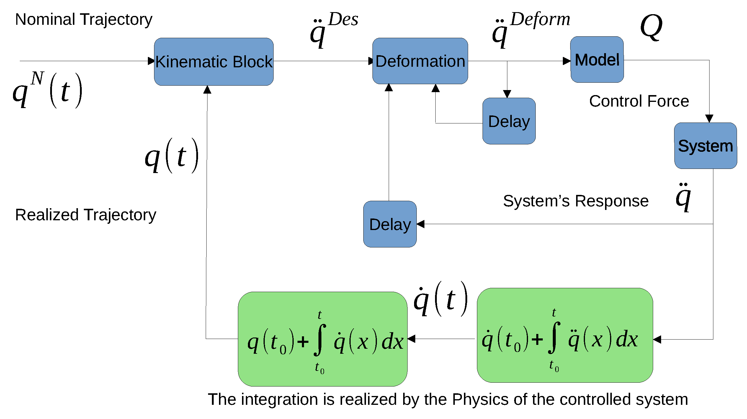
To tackle the problem of the “transient behavior” of the controlled system that is not clearly addressed in the approaches that guarantee only the stability of the solution, in [21] a novel iterative controller was suggested in which the task of computing the appropriate control signal was transformed to finding the fixed point of a contractive map. Its structure for a second-order physical system is sketched in Figure 1.
It is a “flexible framework” that can be filled in with various particular contents. In the “Kinematic Block”, an arbitrary tracking strategy can be formulated that can drive the trajectory tracking error to 0 as . For instance, in a “Proportional, Integral, Derivative (PID)” design the following quantities can be introduced with a positive constant in (1). Its stability can be proved without the use of any Lyapunov function.
It is evident that the functions have the property in (2)
therefore the linear space of the general solution of the LTI system in (1c) can be spanned by three basis functions of which each converges to 0 if in the form given in (3)
in which the constants are determined by the arbitrary initial conditions. The basis function is mapped to zero by the operator , is mapped to zero by , and finally is mapped to zero by . It is evident that not only converges to zero: and also have to converge to zero because a sequence of implications can be obtained that “after a while” (practically a few times ) various components will become 0 as in (4)
Evidently, (4b) can be rewritten in the form of (5) that corresponds to a stable inhomogeneous system in which due to (4d) the inhomogeneous “driving term” will vanish after a while, therefore as
In similar manner (4a) can be rewritten as (6)
that again is a stable inhomogeneous LTI system in which the inhomogeneous driving terms vanish after a while, therefore as .
In the case of digital controllers, the box “Delay” normally corresponds to the cycle time of the digital controllers. In the box “Deformation”, the “Response Function” of the system can be introduced as in which the variables in the position denoted by the symbol “…” only slowly can vary while the controller very quickly can modify . The box contains the function or that is so constructed that if then , that is, the solution of the control task is the fixed point of function G. For the construction of G various proposals were put forward and investigated in [21,22,23] by the use of functions in analytical form. For proving the convergence of the iteration Banach’s fixed point theorem [24] was used according to which in a linear, normed, complete metric space (“Banach Space”) the iterative sequence created by the contractive mapping as converges to the unique fixed point of the function . For this purpose the response function generally has to meet the condition that the real part of each eigenvalue of must be negative or positive simultaneously in the vicinity of the fixed point. In this case, it is possible to introduce appropriate parameters in the function G that can guarantee its contractivity [25]. Though during one digital control step only one step of this iteration can be performed, since and vary only very slowly in comparison with , according to ample simulation investigations, this method showed good convergence properties in many cases. The proofs were based on Taylor series approximation of the function values in the vicinity of the fixed point. By realizing similar deformation in the field of the control forces the fixed point iteration-based method was found applicable in a novel design of MRAC controllers [26]. It was shown that this novel technique could be interpreted from the point of view of the Lyapunov function, too [27,28].
In [29] a simple, geometrically interpreted method was introduced. The arrays , can be so augmented to arrays , that they obtain a common Frobenius norm: . If these vectors are not parallel to each other they span a 2 dimensional hyperplane in that is also spanned by the orthogonal unit vectors and that is made of the component of that is orthogonal to . In this case the skew-symmetric matrix and the angle determine an Orthogonal Matrix that makes rotations in the space so that the ‘‘axis of rotation” is the dimensional orthogonal subspace of the vectors
that corresponds to the generalization of the Rodrigues formula [30] (this fact easily can be proved by utilizing that ). If is calculated from the scalar product as , just rotates the augmented vector into the other augmented vector . Consequently, the physically interpreted projection of , is exactly transformed into . By the introduction of an interpolation factor the rotation with makes approach . When this function is applied in the block called Deformation, via setting a great value to R and a small one to , the convergence of the iteration can be guaranteed if the angle formed between and is acute. The steering systems of bicycles and cars work accordingly: if the driver wishes to achieve “sharper turn” to the tune of , the necessary modification of the rotational angle of the steering wheel, i.e., , forms an acute angle with . In other words: if the driver wishes to turn to the left, the steering wheel has to be turned to the left, too. This simple property can be well utilized in the practice in the development of steering algorithms.
With regard to modeling issues, the pioneering discovery by Weierstraß has to be mentioned. In a lecture in 1872 he gave the first example for an everywhere continuous function that nowhere was differentiable [31]. He highlighted the fact that the class of continuous functions is so complicated that we cannot even “imagine” the graph of a general continuous function. We can “see” only the graphs of “smooth” functions the derivatives of which may have some jumps at a few discrete points only. His discovery anticipated difficulties in the field of approximation of continuous functions; however, in his inaugural lecture at the Academy of Berlin in 1885 he has shown that polynomials can be regarded as universal approximators of single variable continuous functions [32]. His theorem was extended from polynomials to other approximators by Stone in 1948 [33]. The approximation of multivariable continuous functions was found to be a more difficult task. In around 1900, Hilbert in one of his conjectures “guessed” that it was impossible to construct continuous multivariable functions by the use of single variable ones [34]. Though in 1927 Volterra introduced a series model [35] that is a sequence of approximations for continuous functions using a polynomial functional expansion [36] for dealing with integro-differential equations, the first rigorous rebuttals of Hilbert’s conjecture were published only in 1957 by Arnold for the functions of three variables [37], and by Kolmogorov for continuous functions of many variables [38]. Kolmogorov’s constructive proof in the 1960s was simplified and made more elegant by Sprecher in 1965 [39] and Lorentz in 1966 [40,41], and served as the mathematical background of the feedforward neural networks that can be regarded as technical realizations of the universal approximators that appeared in the 1990s [42,43]. In 1990, the idea of “Convolutional Neural Networks (CNN)” was suggested for image recognition applications by Le Cun et al. [44] in which a convolutional layer was the fundamental building block. The early convolutional layers were linear systems: their outputs were affine transformations of their inputs. To take into account nonlinear effects in face recognition, the Volterra polynomials appeared in 2009 in [45], and later were built in the CNNs [36], too. While the feedforward neural networks can be taught by examples, Kohonen’s “self-organizing map” [46] was able to automatically find categories in samples. For modeling dynamic effects, recurrent neural networks appeared [47,48] and were introduced in the CNN’s convolutional layer [49], too.
For the mathematically rigorous tackling of uncertainties of non-statistical nature in 1965, Zadeh introduced the concept of “fuzzy sets” [50]. By our time, the concept was extended to “type 3” sets [51]. In the 1990s, it became clear that the fuzzy systems can be regarded as universal approximators, too [52,53], in which the Weierstraß–Stone approximation theorem can also be used [54]. Practically satisfactory description of the physical state of certain machines as e.g., turbojet engines, various parameters as temperature, pressure, speed, and vibrations are used that can be revealed by complicated diagnostic methods (e.g., [55,56,57]); however, for control purposes, only certain aspects of the “complete” physical model can be used (e.g., [58,59]) in the form of very “incomplete” models.
From the point of view of function approximation, the various realizations of the universal approximators can be regarded as huge structures that contain numerous free parameters that have to be fitted. For this purpose, numerous methods, such as the gradient descent type “error backpropagation” [60] that can be made more efficient by using appropriate activation functions in the neurons, its combination with genetic algorithms [61], other stochastic optimization methods as simulated annealing [62], memetic algorithms and bacterial memetic algorithms [63,64,65,66], simplex algorithm [67,68,69], “particle swarm algorithm” [70,71], etc., can be mentioned.
Rigorous theoretical investigations soon revealed the phenomenon called “curse of dimensionality” due to which the “universal approximator” ability of the soft computing tools was doubted at least from practical point of view (e.g., [72,73,74]). Much of these problems in terms of “nowhere denseness” stem from the “irregular nature” of the continuous functions discovered by Weierstraß in [31]. It can be expected that the situation is not so hard in the case of “smooth functions”. In this view, the idea of “polytopic models” was introduced in 2006 [75,76] in which the function values were sampled over some grid points of a multidimensional space (i.e., in the vertices of polytopes). By the use of the higher-order generalization of Golub’s and Kahan’s “Singular Value Decomposition (SVD)” [77] by Lathauwer et al. in 2000 [78], these models can be simplified by finding the most important contributions belonging to the larger singular values, under well controlled conditions. Further, by also taking into account control possibilities via “Linear Matrix Inequalities (LMI)”, the controller design methodology of the “tensor product model” was proposed in [79]. This approach renders the program announced by Boyd et al. in 1994 [80] generally applicable. By the use of LMIs a wide set of control problems can be solved by a Lyapunov function-based design, for which efficient MATLAB packages were developed [81]. In this approach, in each cell different metric tensor can be applied in the Lyapunov function. Passing the cells’ limits can make certain problems arise that can be tackled by the use of either “switching controllers” (e.g., [82,83,84]) or some redundant system of coordinates can be used from the vertices of a polytope within a convex hull to deal with a continuous problem (e.g., [85]).
To tackle the problem of the curse of dimensionality, to evade the need for massive parallelism and sophisticated data synchronization in the learning and operating phases of the traditional structures, in [86], a novel soft computing structure was suggested that is more or less akin to a coarse resolution grid or a fuzzy model in which very approximate and simple rules are applied for control purposes. It broke with the Lyapunov function-based design that generally was present in the switching controllers and in the “Linear Parameter Varying (LPV)” or “Quasi LPV” design by the application of simple smoothed tracking of the jumps in the control force. At first, its modeling ability was checked for the description of the behavior of the free and the controlled van der Pol oscillator [87] that is a popular benchmark system. It makes nonlinear oscillations in a limit cycle. For modeling the motion of the free system, the function , and for control purposes, the function , were approximated in a dynamic range that was “filled in” during the control process. It had the main properties as follows:
- 1.
- For the free system, the two dimensional vectors and were augmented to three-dimensional ones of identical Frobenius norms and exactly as it was performed in the rotations-based abstract deformations applied in [29]. In the case of the controlled model the three-dimensional vectors and were similarly augmented to produce the four dimensional ones of identical norms as and in which and were the “dummy components” without any physical interpretation. Their role was to guarantee equal norms.
- 2.
- Coarse resolution grids were introduced in for the values, and in for the values. In the center points of the grids, the appropriate and Q values were computed from the available exact model of the van der Pol oscillator. Following that, the abstract rotations defined in (7) were calculated that rotated into , and transformed into , respectively. Each grid cell was associated with a “neuron” that had the “activation function”. It executed the rotations according to (7), and had the following parameters:
- Its cell-limits as , for the free motion, and , , for the controlled system, respectively;
- The orthogonal unit vectors and of which the generator of the rotation in (7) can be computed, and the angle of the necessary rotation, .
- 3.
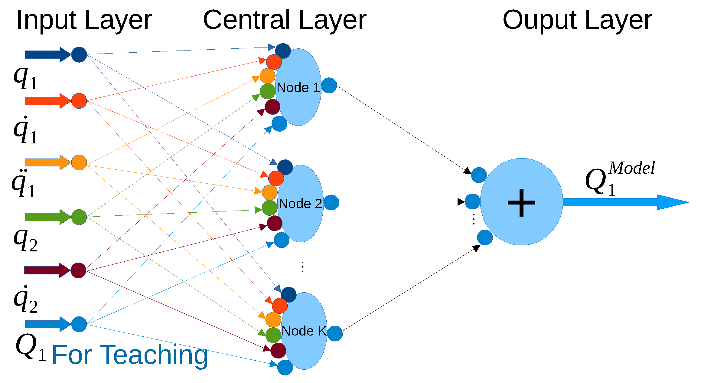
- These neurons were arranged in a single layer in which each neuron obtained its input value for the “teaching process” as for the free system, and for the dynamic model. If the input signal belonged to the “range of competence” of the given neuron, , , and were computed. During the “normal operation” the neuron used the input for the free system modeling as and for “the use for control mode”. If the input data belonged to its range of competence, it computed , computed the rotated vector for the free system, and for the control application, and as its output, it provided the first component of the rotated vector that corresponded to the modeled value of and Q, respectively.
- 4.
- The last layer of the novel neural structure consisted of a single neuron that summarized the calculated outputs. Since the cells’ limits were determined in a way that the model had only disjoint cells, the output of the summarizing layer was the result of the “soft model”.
- 5.
- To reduce the effects of the jumps in the control signal at the cell boundaries, the really applied generalized force was smoothed by the tracking rule based on a positive constant in (8)that, for a stationary “driving term" , has the stationary solution , furthermore, for time-varying , two different solutions of (8), i.e., and , can differ from each other by that satisfies the differential equation , that is, the differences can stem from the initial conditions and converge to 0 as . Consequently, the smoothed signal tracks well the actual if the variation of which is not significant during the time-interval of duration , and “smooths well” the signals that have faster variation.
- 6.
- The data representation made it possible to apply real-time modification (“step-by-step learning”) of the neuron’s previously learned parameters as the unit vectors , and were refreshed according to a learning rule determined by the parameter asIt must be noted that even if and were orthogonal to each other, the new unit vectors and will not be exactly orthogonal ones. Consequently, the new skew symmetric matrix can generate rotations in the form , but, because , instead of (7) we can state only thati.e., by maintaining the right-hand side of (10) that is easy to compute, instead of exact rotations, linear transformations can be used that are good approximations of rotations.
In the present paper the above outlined idea is extended and it contains the novelties as follows:
- 1.
- The controlled system is an underactuated two degree of freedom construction in which the directly controlled subsystem is dynamically coupled with a non-controllable one acting as “parasite dynamics”.
- 2.
- Instead of the simple CTC control and its robust variable structure/sliding mode-based correction (e.g., [88,89,90]), the “fixed point iteration-based adaptive control scheme” depicted in Figure 1 is applied to compensate the effects of the imprecisions of the coarse grid-based model with the application of the rotations-based adaptive controller announced in [29].
- 3.
- The effects of the measurement noises are investigated and reduced by a smoothing technique that is similar to the solution published in [91].
- 4.
- The computation time of the controller was measured for the hardware and software environment that was used in the simulations.
2. The Dynamic Model of the Controlled System
The controlled system is a wheel that is rotated around a horizontal axle. In one of its spokes, a mass point is built in. It is located between two springs and its motion is damped by viscous friction. The Euler–Lagrange equations of motion of this model are completed with the friction term and are given in (11) that can be used for simulation purposes,
in which denotes the rotational angle of the wheel, is the radial distance of the mass point along the spoke, measured from the rotational axle, r is the zero force position of the spring connected the axle with the mass point, k is the spring constant, d denotes the viscous damping coefficient of the mass point as it moves along the spoke, m is its inertia, and corresponds to the inertia momentum of the wheel, denotes the driving torque. For control purposes, the necessary control torque can be obtained by rearranging (11a) as
The numerical data used in the simulations are given in Table 1.
3. The Rotational Neural Model Structure Tailored to the Controlled System
The structure of the rotational neural model is outlined in Figure 2.
The nodes corresponded to 11 elements grids as follows: with the grid width , with the grid width , with the grid width , with the grid width , with the grid width . For smoothing the torque signal obtained from (8) the parameter was in use. The augmented vectors were rotated in with the common vector norm . The adaptive rotations in Figure 1 were achieved in the space with the common vector norm and interpolation factor . For incremental learning purposes in (9) was used. In the “Kinematic Block" of Figure 1 the PID term with was applied.
With regard to noise issues, it was assumed that was measurable in each digital cycle with a Gaussian noise of and was measurable with a Gaussian noise of . For filtering the measurement noises, the measured noisy signal x was tracked by the filtered one according to the tracking rule given in (13)
and the filtered values were used in the “Kinematic Block" and in the fixed point iteration with the filtering parameter . The operation of this filter can be analyzed exactly as it was performed in the case of (8).
4. Simulation Results
Numerical simulations were performed by the use of the Julia language Version 1.5.1 (25 August 2020) working under the operating system Linux 5.10.53-1-MANJARO x86_64 21.1.0 Pahvo on a DELL inspiron 15R laptop using the program code that is available on the Web given in Section “Sample Availability": “Wheel_Applied_Sciences_Noisy.jl”.
4.1. Comparative Analysis of the Performances of the Neural and the Exact Models
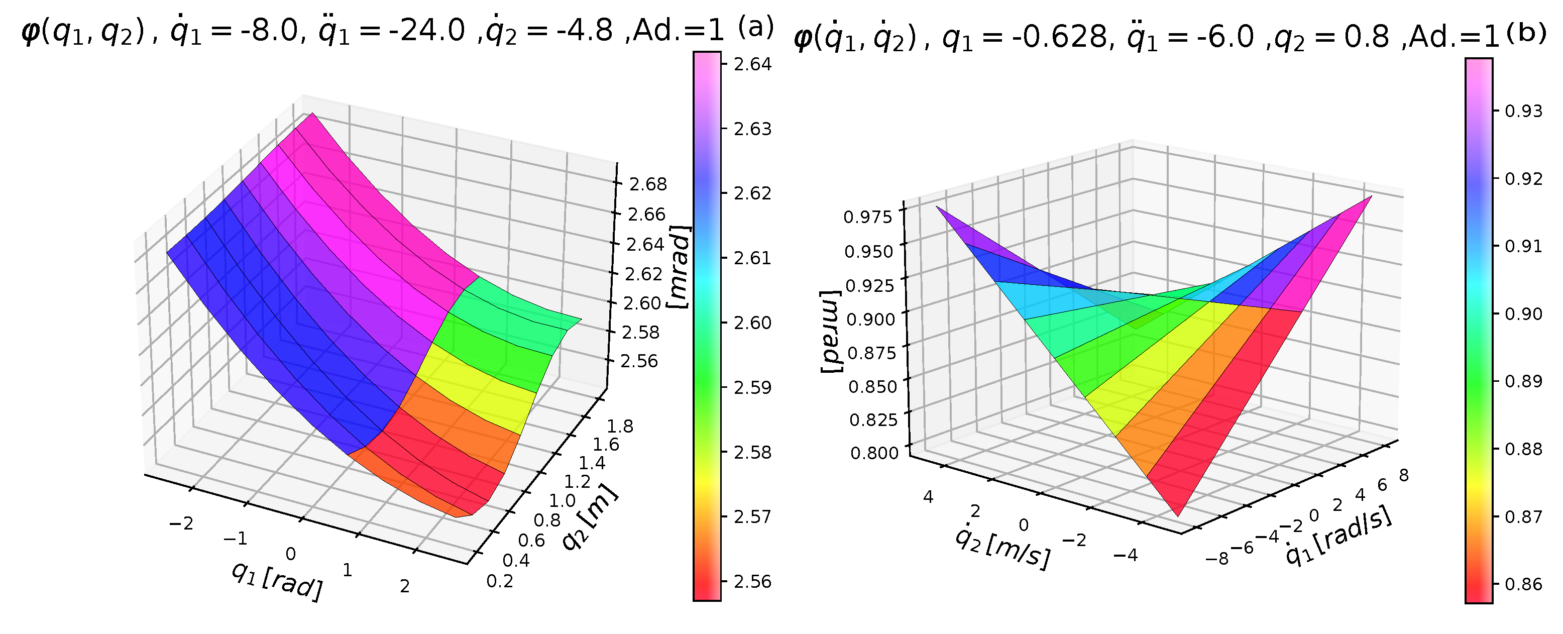
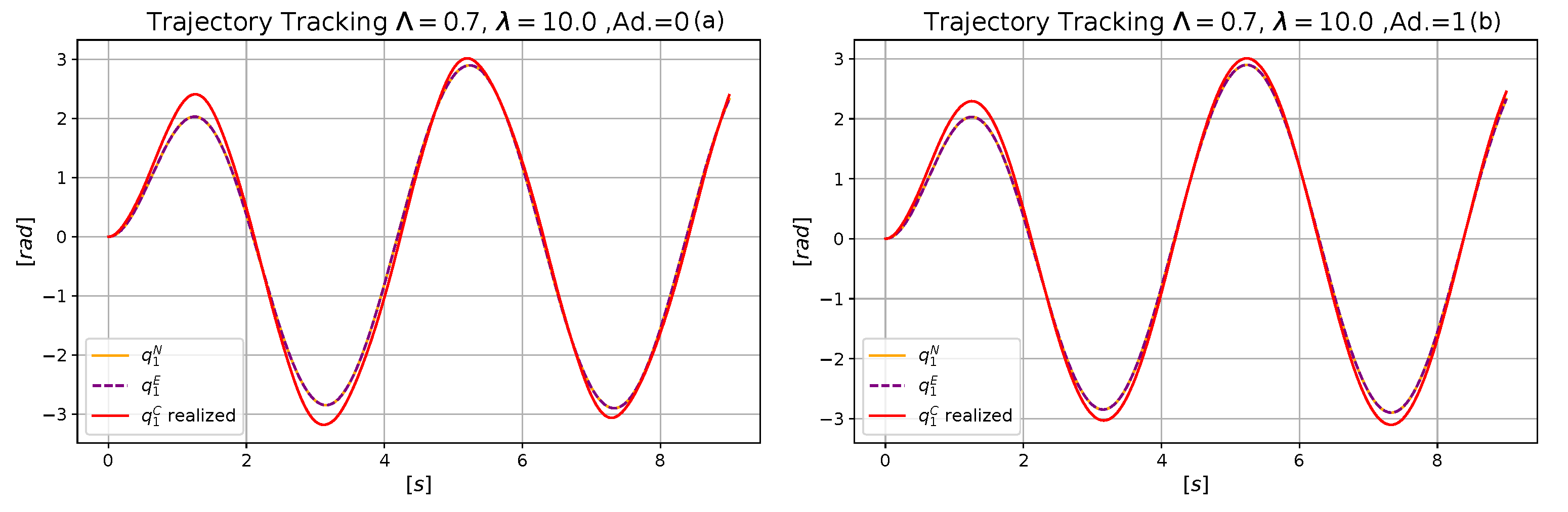
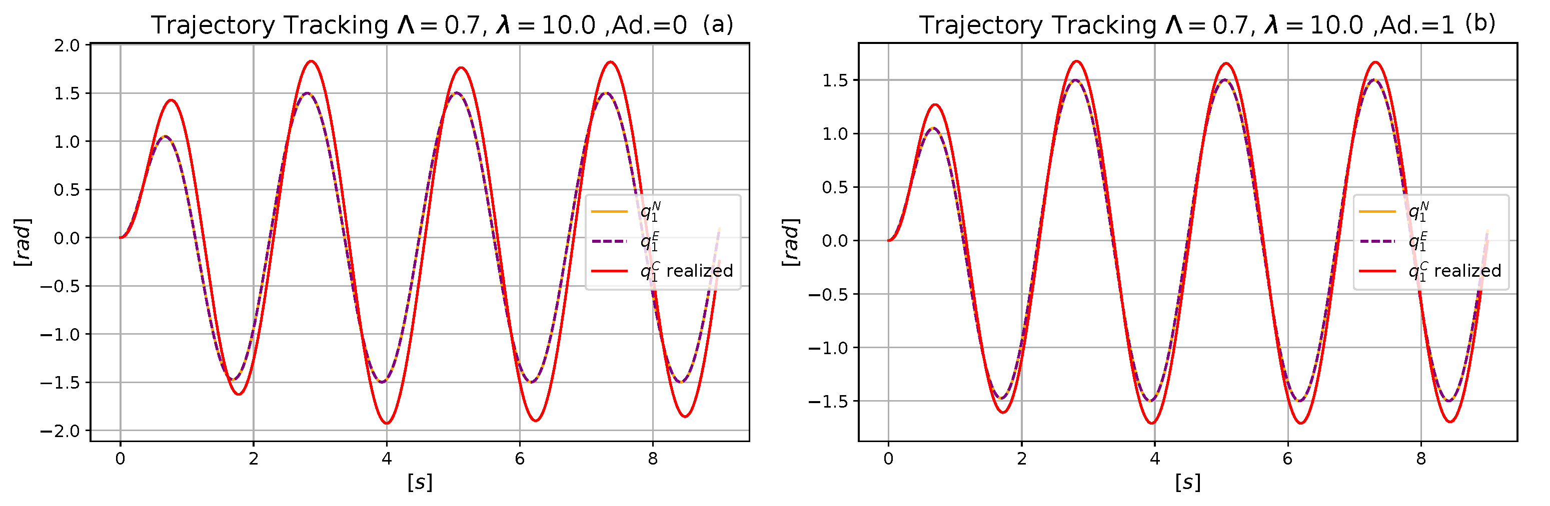
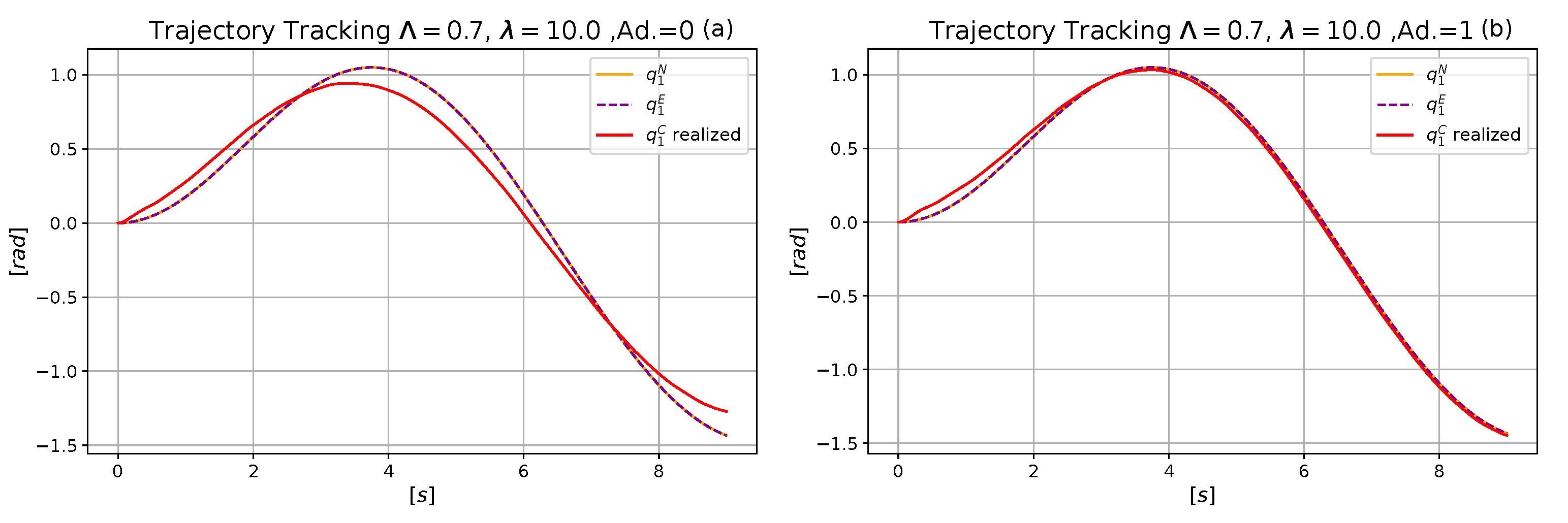
In this subsection, the figures also contain simulation results obtained when the exact dynamic model was in use to support comparative analysis. In Figure 3, two 2-dimensional sub-spaces of the stored “soft dynamic model” in are exemplified by giving the stored abstract rotational angles of the rotations in the augmented space. The non-adaptive control corresponds to the simple CTC controller. In Figure 4, the trajectory tracking properties can be compared.
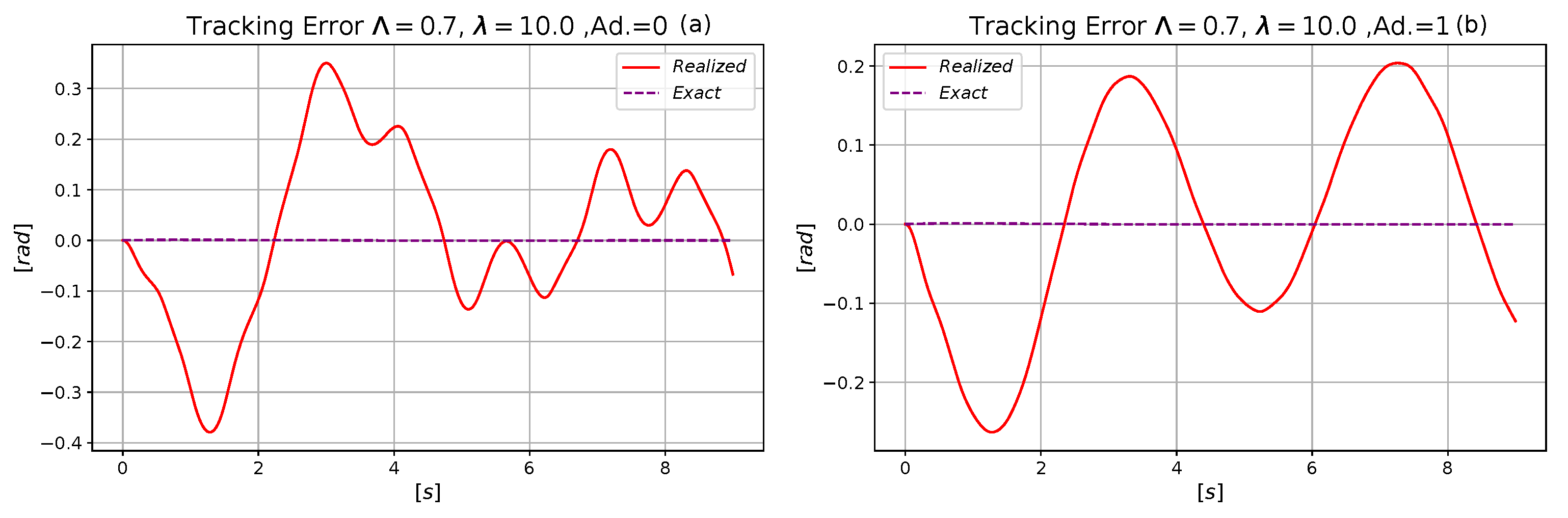
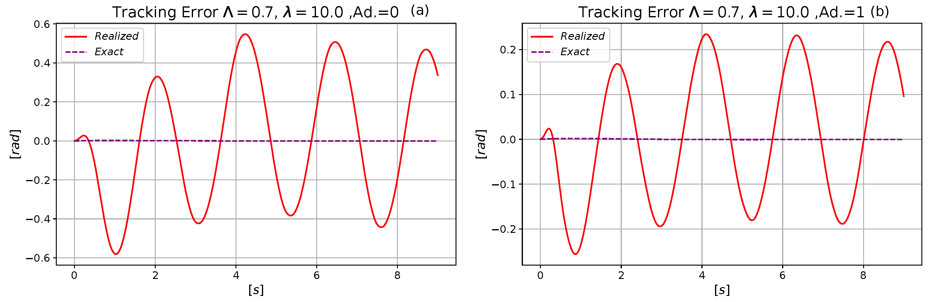
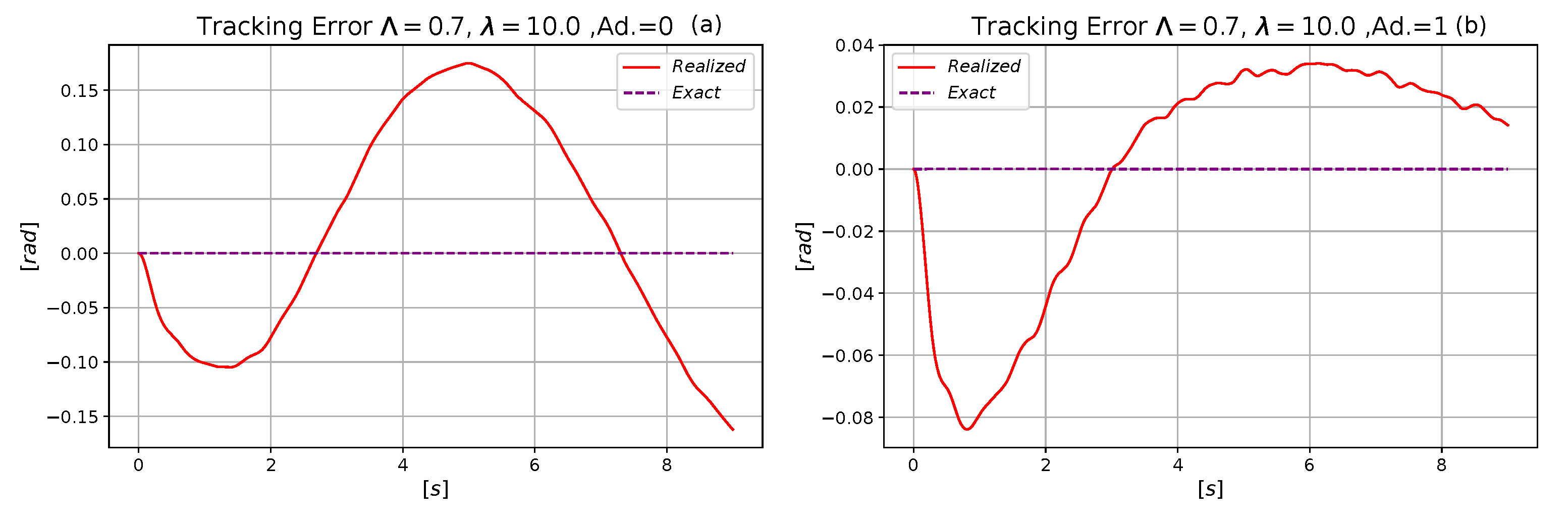
Figure 5 reveals that the adaptive control evades the greater tracking errors.
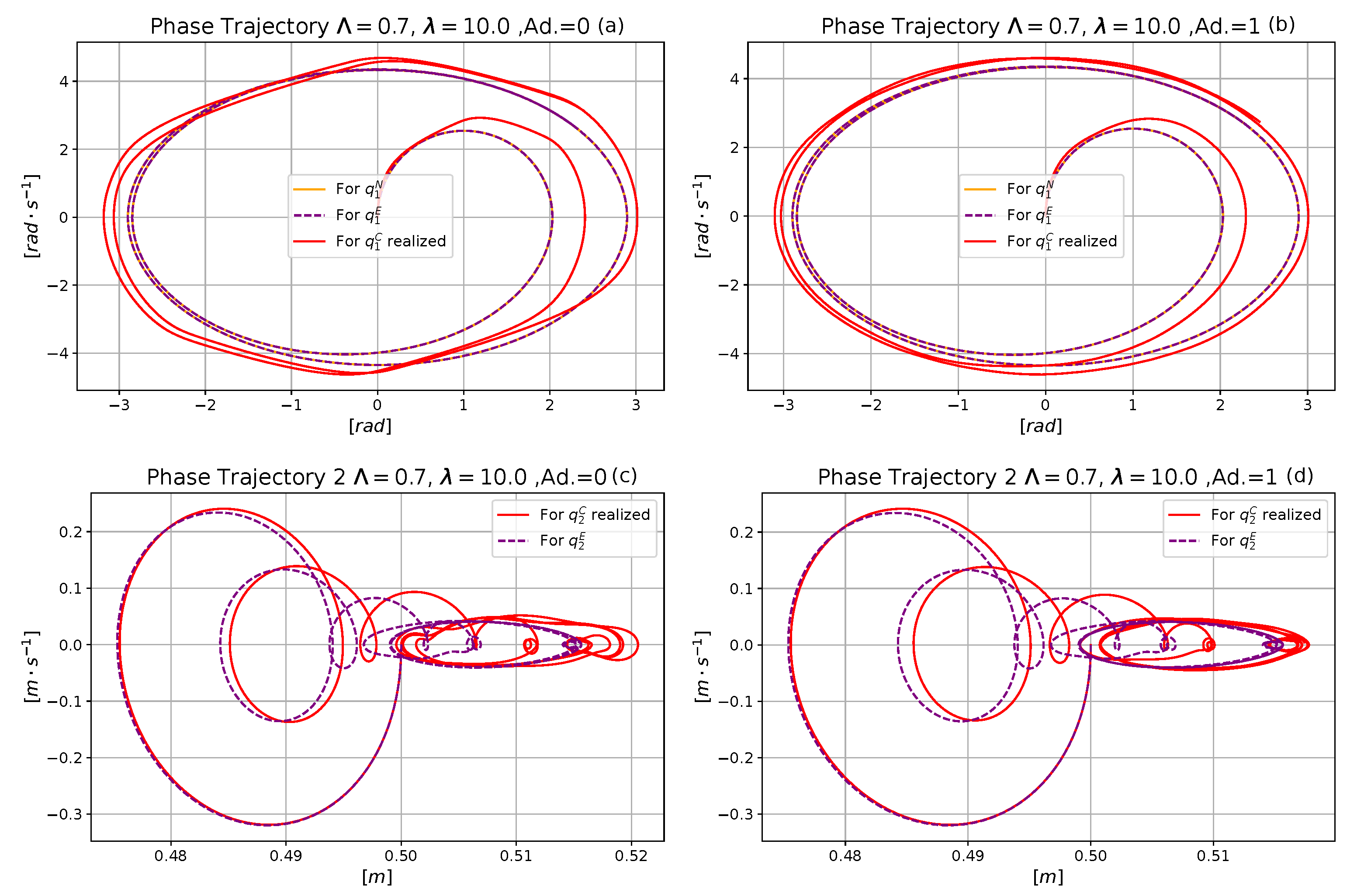
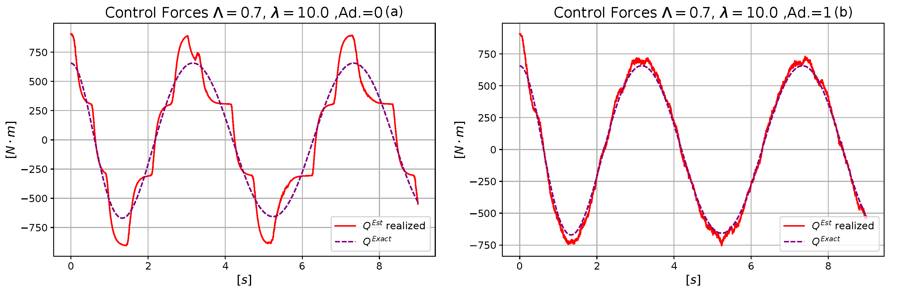
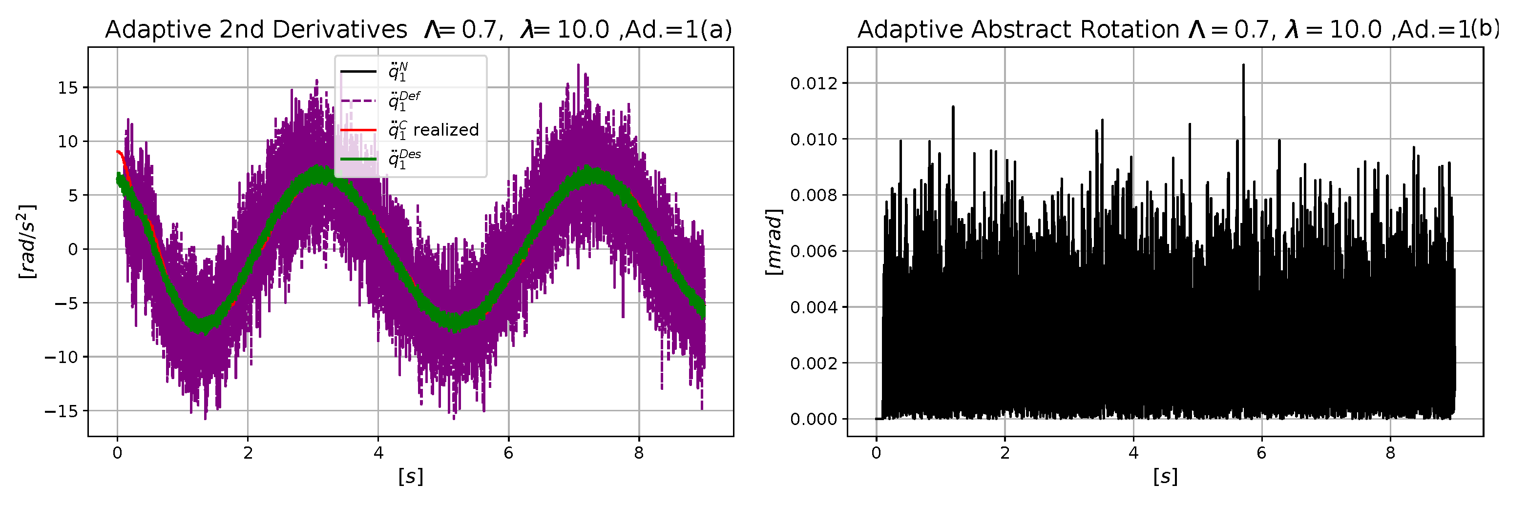
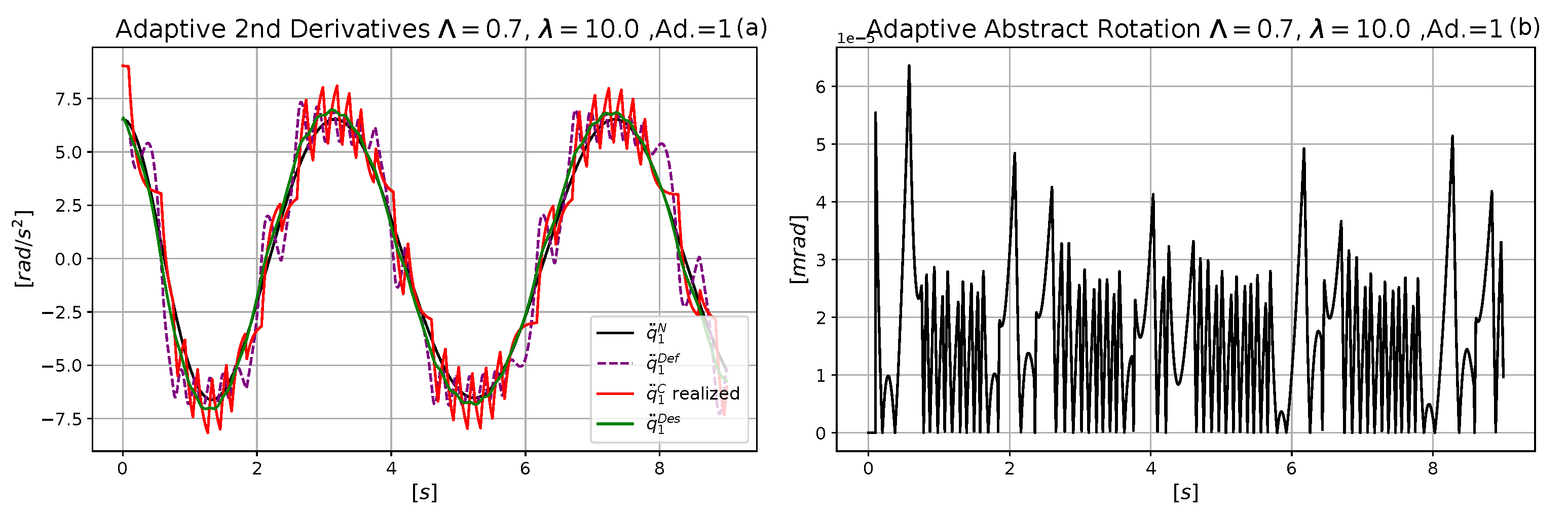
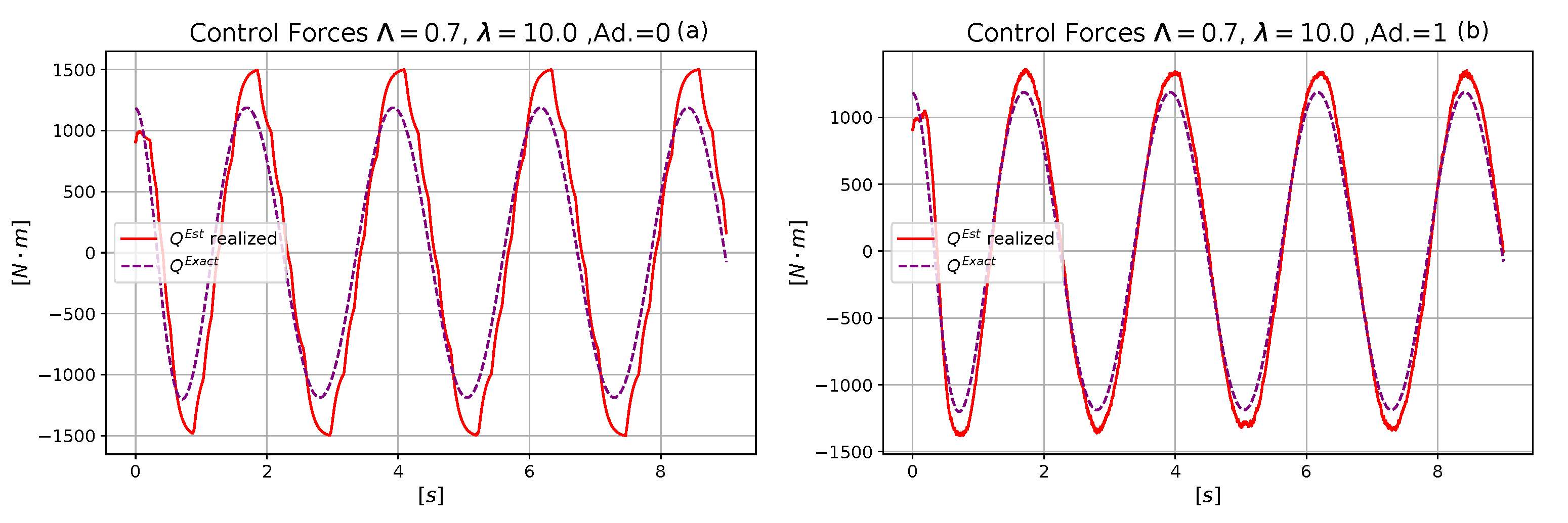
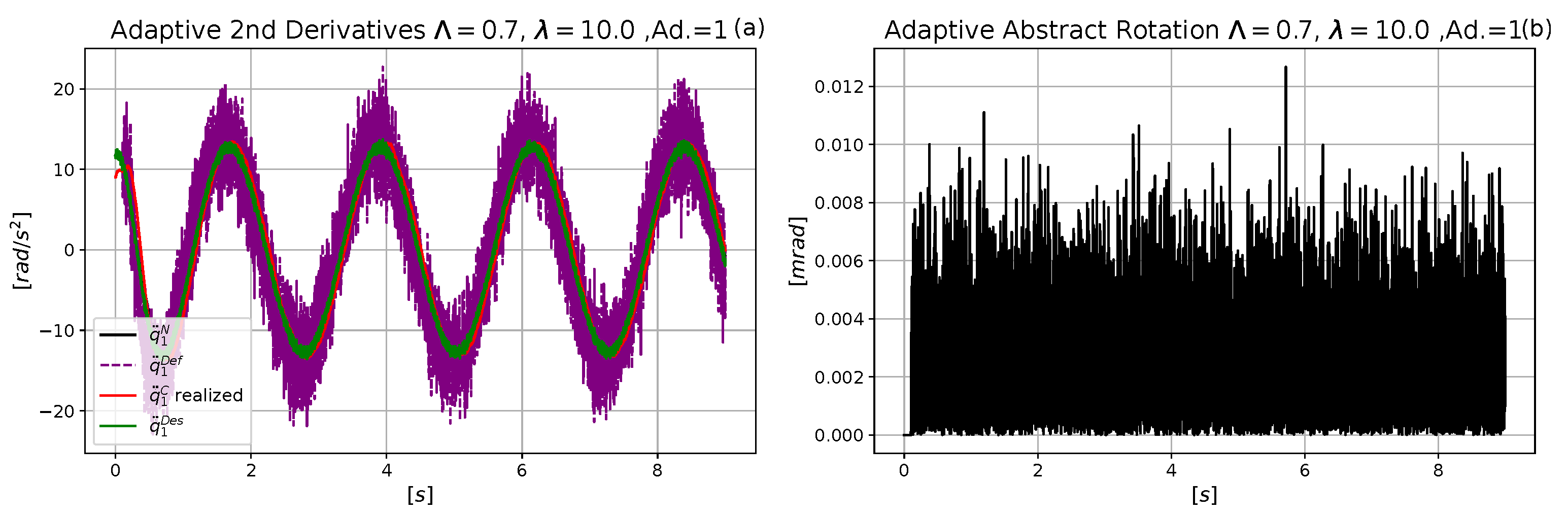
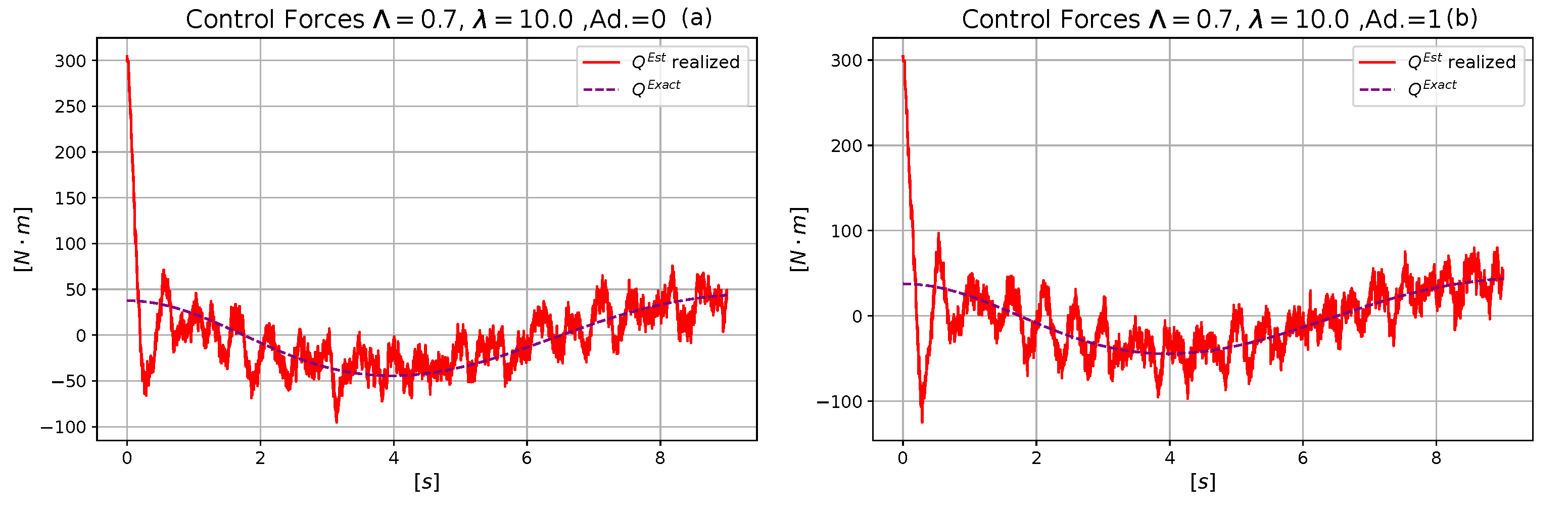
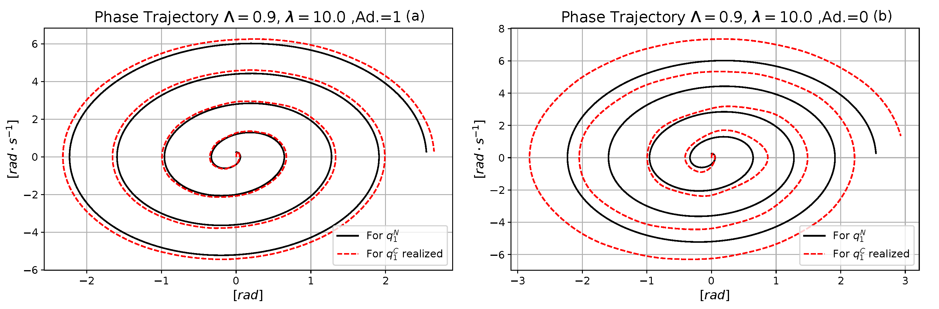
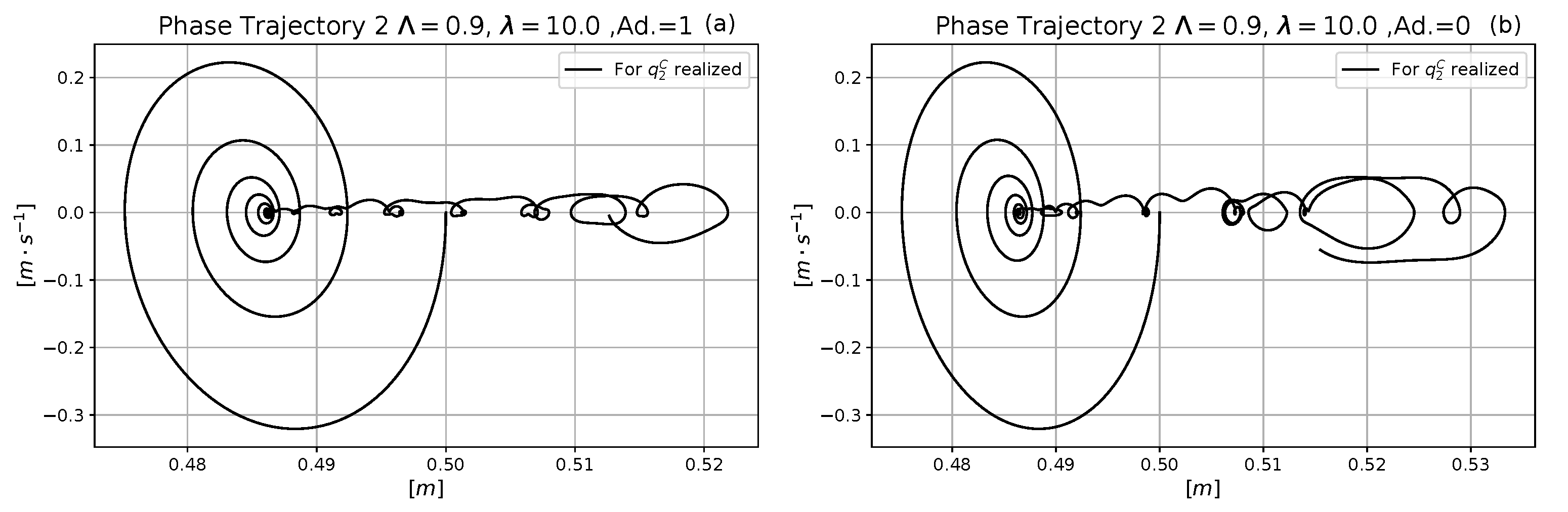
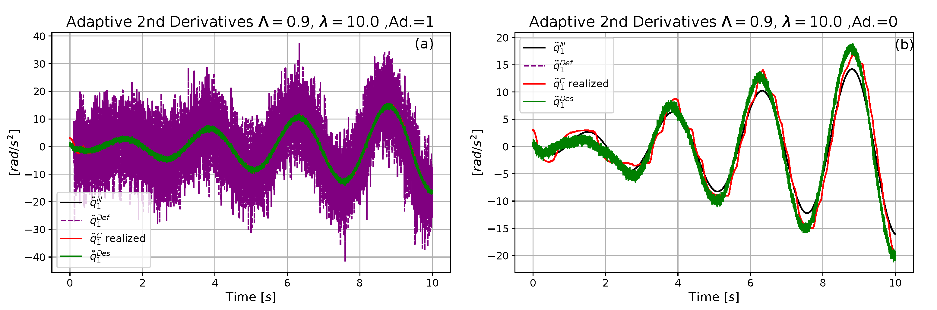
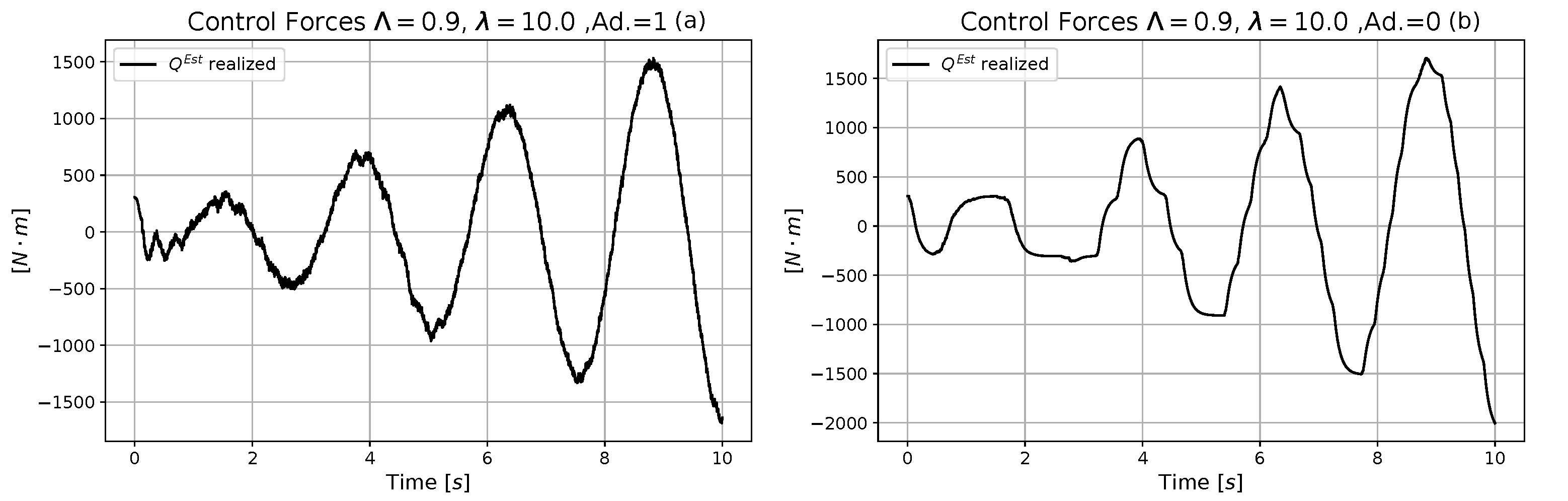
According to Figure 6, the adaptation makes the phase trajectory of the controlled system “more canonical” and reduces the excitation of the coupled parasite dynamical subsystem. According to Figure 7, the adaptive approach causes more even control torque contributions in spite of the noisy signals. In the non-adaptive results, the effects of changing the cell that is competent to fire can be identified. The dynamic range of the adaptive control forces is considerably narrower than that of the non-adaptive control. Figure 8 reveals the operation of the adaptive controller: due to the adaptive deformation, the realized 2nd time-derivative values well approximate the desired ones. This effect can be observed better in the lack of measurement noises in Figure 9.
4.2. Estimation of the Computational Time of the Operations in the Control Cycles
Computational complexity of the suggested method and the duration of the necessary computations within the control cycles is an interesting practical question. It cannot be estimated by counting the necessary mathematical operations, because it depends on various external factors, such as the operating system that manages the controller, and the properties of the program that realizes the control task. Normally, a multitasking controller is available that uses a single central processor unit. Its capacities are shared by various cooperating processes. If the operating system is not definitely designed to manage real-time tasks, the actual duration of a given computation depends on the other duties of the computer. For instance, if during the calculation of the simulations some video player is in use, its effects can be well observed in the duration of each actually executed computation.
In a similar manner, if the program language makes “garbage collection” in the stack, such an activity may need considerably longer time than that of a “normal computation” within the control cycle. These longer sessions, though not very frequently, sometimes appear during the simulation. The Julia language is a typical garbage collecting construction that generates such effects.
However, it offers a simple solution to measure the time that is needed for the operations defined in a given command line. For instance, the command “a+=@elapsed b=myfunc(-12.1)” adds to the content of variable “a” the computational time (in seconds) of the following steps: the function “myfunc” is called with the input argument -12.1 and its output is stored in variable “b”. The time-need of a bigger unit as e.g., “a+=@elapsed for...end”, “a+=@elapsed while...end”, etc. can be measured in similar manner.
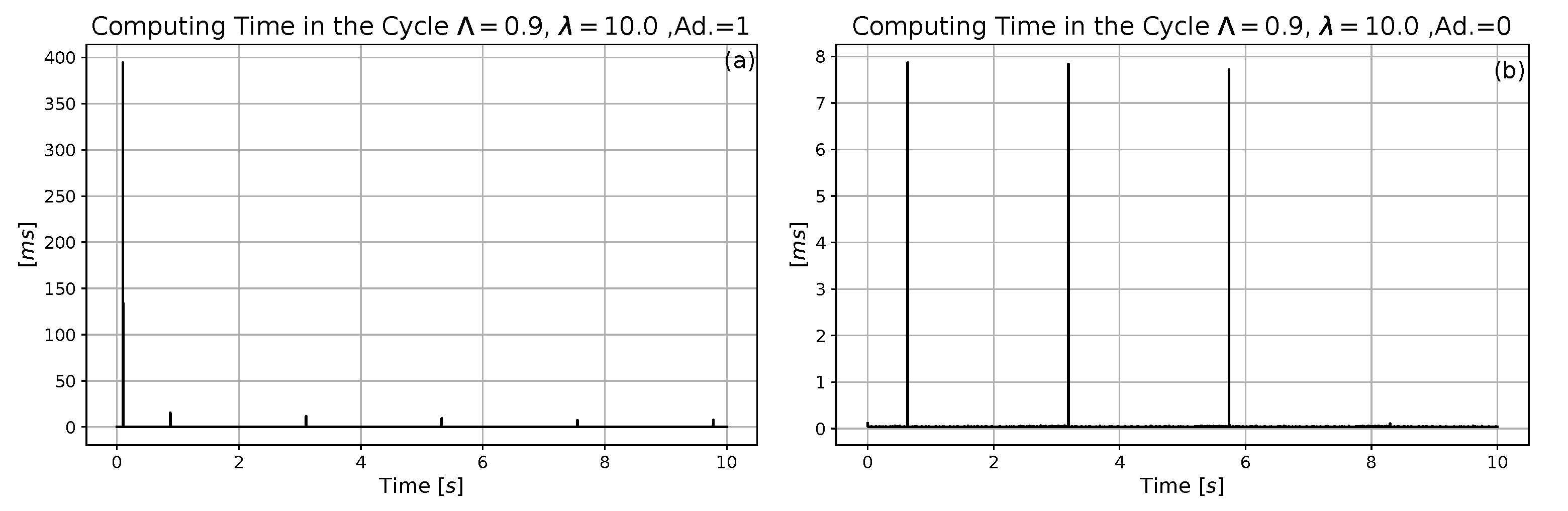
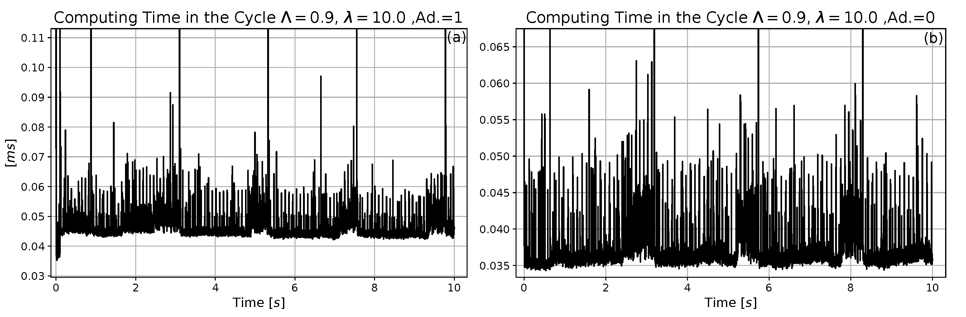
A program code “Wheel_Applied_Sciences_Noisy_Computing_Time_New.jl” that utilizes this possibility (also available in the Web) was made in which the time needed for the essential computations within each control cycle was summarized. In these investigations, the parameter settings and were used, all the other control and model parameters remained invariant. In this program, no computation was made for the operation of the “exact system"-based control. The nominal trajectory had time-dependent, increasing amplitude. During the calculations, only the console running Julia was in operation, a text editor in which the program file was kept opened, and the standard Internet connection was kept running. In the sequel, results obtained for the adaptive and non-adaptive controllers are discussed. Figure 17 reveals a few huge peaks that certainly cannot belong to the essential computations. The important information can be seen in the “zoomed-in excerpts” of the graphs displayed in Figure 18.
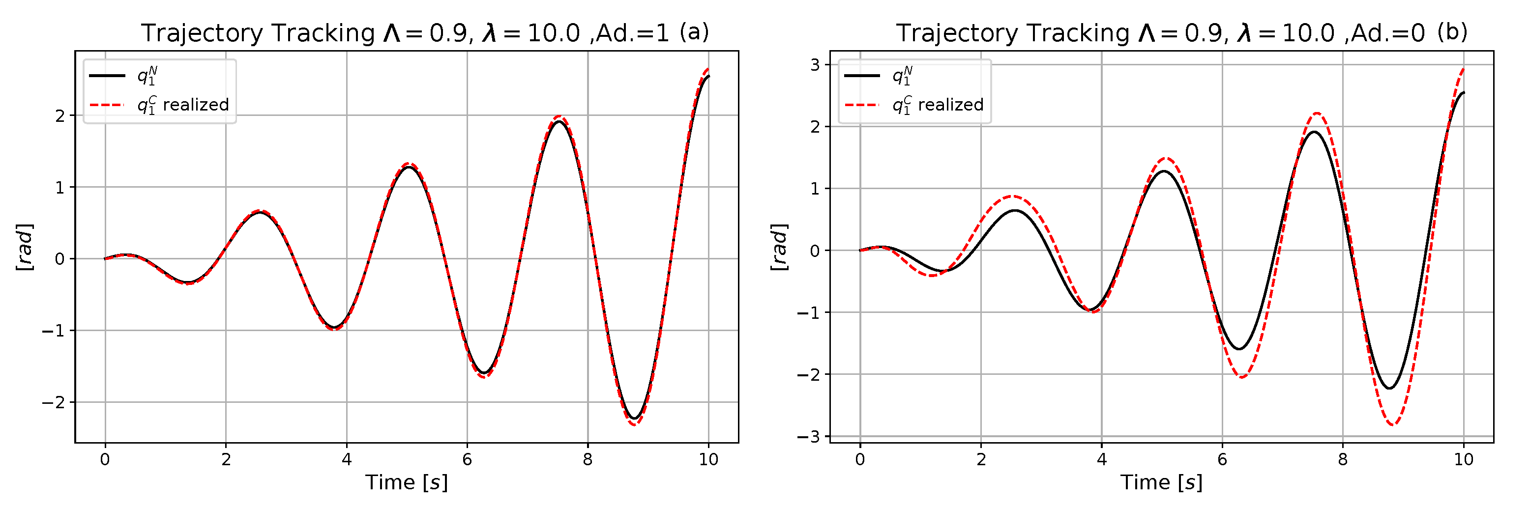
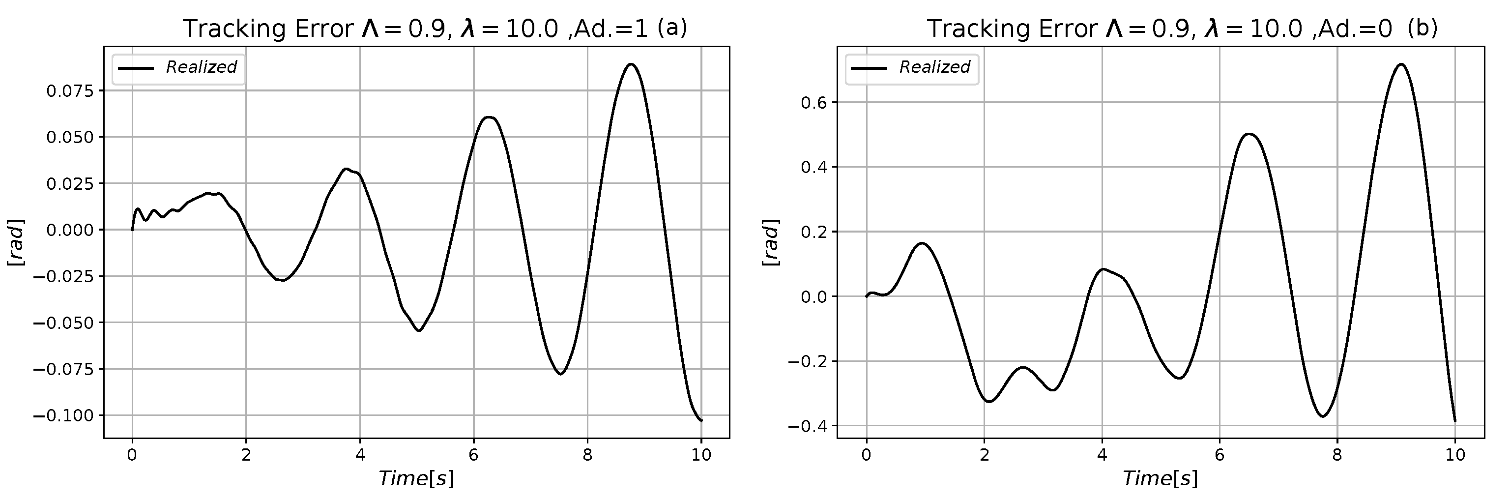
It is evident that during one digital control step of duration of the non-adaptive computations needed less than , while the adaptive ones consumed up approximately maximum . This observation indicates that the suggested method can be implemented by the use of common hardware/software tools. Figure 19 and Figure 20 compare the trajectory tracking performances. In Figure 21 and Figure 22 the phase trajectory of the controlled and that of the coupled “parasite system” can be seen. These figures well reveal the effects of the necessary centripetal force that increases with the amplitude of the nominal motion.
5. Discussion
In this paper, the idea of “rotational neural networks” introduced in [86] was applied to bring about a coarse grid-based soft dynamic model for control applications. The jumps in the model output at the cell boundaries are smoothed by a first-order tracking controller, and the effects of the model inaccuracies are compensated by a fixed point iteration-based adaptive controller. Both the adaptive and modeling mechanisms are based on the same mathematical background that applies simple rotations in higher dimensional spaces. It was shown that the network is able to work in a “step-by-step” learning mode in which the information stored in a visited cell can be refined depending on the fact that various parts of the coarse resolution cells can be visited during the motion of the controlled system.
The suggested network has very simple topological structure and it is easy to simulate it, too. It was shown that the modeling and control methods can be combined with simple noise filtering techniques. The operation of this controller seems to be simpler than that of the traditional fuzzy controller that has to compute ample number of “generalized” maximum and minimum operations over wide ranges.
The most important advantage of this approach is that it breaks with the Lyapunov function-based design in which the phenomenologically well interpreted error components, their integrals and derivatives are “mixed” by the use of very special metric tensors so that these metrics as they are do not have clear interpretation and physical meaning. In the novel approach for each error component kinematically well interpreted behavior can be prescribed.
The applicability of the suggested method was demonstrated in the case of a two degree of freedom underactuated paradigm in which the control of the motion of a wheel is perturbed by a directly not controllable, dynamically coupled parasite system within one of its spokes. The sum of the duration of the necessary computations within each control cycle was calculated for the hardware/software system that run the simulation. It was concluded that at the level of our prevailing possibilities the suggested approach is realistic.
In the simulations, special PID-like kinematic behavior was required that does not result in monotonic decrease of the error components; however, this method can be combined with various fractional order derivatives-based kinematic requirements (e.g., [92,93,94]) that can produce monotonic variation.
In the future, we wish to compare the operation of this idea with that of traditional fuzzy controllers based on approximate and “coarse” rules. For this purpose an electromechanical testbed was built and used for testing the operation of the traditional PID and CTC controllers in [95]. The first successful preliminary results with regard to the implementation of the fixed point iteration-based adaptive controller using abstract rotations on the same testbed were recently obtained by Árpád Varga. The planned future investigations are based on this instrument.
Author Contributions
Conceptualization, J.F.B. and I.J.R.; methodology, J.F.B. and I.J.R.; software, Á.V.; validation, Á.V.; formal analysis, J.K.T.; writing—original draft preparation, J.K.T. All authors have read and agreed to the published version of the manuscript.
Funding
This research was funded by the Doctoral School of Applied Informatics and Applied Mathematics of Óbuda University, Budapest, Hungary.
Institutional Review Board Statement
Not applicable.
Informed Consent Statement
Not applicable.
Data Availability Statement
The study did not report any data.
Acknowledgments
The authors wish to express their thanks to Krzysztof Kozłowski with whom they were in active working connection and cooperation with from the 1990s in bilateral cooperation projects as well as in relation to the RoMoCo and MMAR conferences. Professor Kozłowski was external member of the Antal Bejczy Center for Intelligent Robotics of Óbuda University, Budapest, Hungary.
Conflicts of Interest
The authors declare no conflict of interest.
Sample Availability
Sample program “Wheel_Applied_Sciences_Noisy.jl” available at “https://drive.google.com/drive/folders/1qh-yUtb-jxLos-rbhL4Jk5diJ3x1HHpp?usp=sharing” (date of last access: 24 August 2021).
References
- Bellman, R. Dynamic Programming and a new formalism in the calculus of variations. Proc. Natl. Acad. Sci. USA 1954, 40, 231–235. [Google Scholar] [CrossRef] [Green Version]
- Bellman, R. Dynamic Programming; Princeton Univ. Press: Princeton, NJ, USA, 1957. [Google Scholar]
- Lagrange, J.; Binet, J.; Garnier, J. Mécanique Analytique (Analytical Mechanics); Binet, J.P.M., Garnier, J.G., Eds.; Ve Courcier: Paris, France, 1811. [Google Scholar]
- Richalet, J.; Rault, A.; Testud, J.; Papon, J. Model predictive heuristic control: Applications to industrial processes. Automatica 1978, 14, 413–428. [Google Scholar] [CrossRef]
- Moldoványi, N. Model Predictive Control of Crystallisers. Ph.D. Thesis, Department of Process Engineering, University of Pannonia, Veszprém, Hungary, 2012. [Google Scholar]
- Pinsker, J.E.; Lee, J.B.; Dassau, E.; Seborg, D.E.; Bradley, P.K.; Gondhalekar, R.; Bevier, W.C.; Huyett, L.; Zisser, H.C.; Doyle, F.J. Randomized Crossover Comparison of Personalized MPC and PID Control Algorithms for the Artificial Pancreas. Diabetes Care 2016, 39, 1135–1142. [Google Scholar] [CrossRef] [Green Version]
- Bellemans, T.; Schutter, B.D.; Moor, B.D. Anticipative model predictive control for ramp metering in freeway networks. In Proceedings of the 2003 American Control Conference, Denver, CO, USA, 4–6 June 2003; pp. 4007–4082. [Google Scholar]
- Muthukumar, N.; Srinivasan, S.; Ramkumar, K.; Kannan, K.; Balas, V. Adaptive Model Predictive Controller for Web Transport Systems. Acta Polytech. Hung. 2016, 13, 181–194. [Google Scholar]
- Reda, A.; Bouzid, A.; Vásárhelyi, J. Model Predictive Control for Automated Vehicle Steering. Acta Polytech. Hung. 2020, 17, 163–182. [Google Scholar] [CrossRef]
- Armstrong, B.; Khatib, O.; Burdick, J. The Explicit Dynamic Model and Internal Parameters of the PUMA 560 Arm. In Proceedings of the 1986 IEEE International Conference on Robotics and Automation, San Francisco, CA, USA, 7–10 April 1986; pp. 510–518. [Google Scholar]
- Sciavicco, L.; Siciliano, B. Modeling and Control of Robot Manipulators; McGraw-Hill: New York, NY, USA, 1996. [Google Scholar]
- Khalil, W.; Dombre, E. Modeling, Identification & Control of Robots; Hermes Penton Science: London, UK, 2002. [Google Scholar]
- Corke, P.; Armstrong-Helouvry, B. A Search for Consensus Among Model Parameters Reported for the PUMA 560 Robot. In Proceedings of the 1994 IEEE International Conference on Robotics and Automation, San Diego, CA, USA, 8–13 May 1994; pp. 1608–1613. [Google Scholar]
- Márton, L.; Lantos, B. Identification and Model-based Compensation of Striebeck Friction. Acta Polytech. Hung. 2006, 3, 45–58. [Google Scholar]
- Canudas de Wit, C.; Olsson, H.; Åström, K.; Linschinsky, P. Dynamic friction models and control design. In Proceedings of the 1993 American Control Conference, San Francisco, CA, USA, 2–4 June 1993; Volume 40, pp. 1920–1926. [Google Scholar]
- Lyapunov, A. A General Task about the Stability of Motion. Ph.D. Thesis, University of Kazan, Tatarstan, Russia, 1892. (In Russian). [Google Scholar]
- Lyapunov, A. Stability of Motion; Academic Press: New York, NY, USA; London, UK, 1966. [Google Scholar]
- Slotine, J.J.E.; Li, W. Applied Nonlinear Control; Prentice Hall International, Inc.: Englewood Cliffs, NJ, USA, 1991. [Google Scholar]
- Nguyen, C.; Antrazi, S.; Zhou, Z.L.; Campbell, C., Jr. Adaptive Control of a Stewart Platform-based Manipulator. J. Robot. Syst. 1993, 10, 657–687. [Google Scholar] [CrossRef]
- Gahinet, P.; Apkarian, P.; Chilali, M. Affine parameter-dependent Lyapunov functions for real parametric uncertainty. IEEE Trans. Autom. Control 1994, 41, 436–442. [Google Scholar] [CrossRef]
- Tar, J.; Bitó, J.; Nádai, L.; Tenreiro Machado, J. Robust Fixed Point Transformations in Adaptive Control Using Local Basin of Attraction. Acta Polytech. Hung. 2009, 6, 21–37. [Google Scholar]
- Dineva, A.; Tar, J.; Várkonyi-Kóczy, A. Novel Generation of Fixed Point Transformation for the Adaptive Control of a Nonlinear Neuron Model. In Proceedings of the IEEE International Conference on Systems, Man, and Cybernetics, Hong Kong, China, 10–13 October 2015; pp. 987–992. [Google Scholar]
- Dineva, A.; Tar, J.; Várkonyi-Kóczy, A.; Piuri, V. Generalization of a Sigmoid Generated Fixed Point Transformation from SISO to MIMO Systems. In Proceedings of the IEEE 19th International Conference on Intelligent Engineering Systems, Bratislava, Slovakia, 3–5 September 2015; pp. 135–140. [Google Scholar]
- Banach, S. Sur les opérations dans les ensembles abstraits et leur application aux équations intégrales (About the Operations in the Abstract Sets and Their Application to Integral Equations). Fund. Math. 1922, 3, 133–181. [Google Scholar] [CrossRef]
- Dineva, A. Non-Conventional Data Representation and Control. Ph.D. Thesis, Óbuda University, Budapest, Hungary, 2016. [Google Scholar]
- Tar, J.; Bitó, J.; Rudas, I. Replacement of Lyapunov’s Direct Method in Model Reference Adaptive Control with Robust Fixed Point Transformations. In Proceedings of the 2010 IEEE 14th International Conference on Intelligent Engineering Systems, Las Palmas, Spain, 5–7 May 2010; pp. 231–235. [Google Scholar]
- Csanádi, B.; Galambos, P.; Tar, J.; Györök, G.; Serester, A. Revisiting Lyapunov’s Technique in the Fixed Point Transformation-based Adaptive Control. In Proceedings of the 22nd IEEE International Conference on Intelligent Engineering Systems, Las Palmas de Gran Canaria, Spain, 21–23 June 2018; pp. 329–334. [Google Scholar]
- Csanádi, B.; Tar, J.; Bitó, J. Novel Model Reference Adaptive Control Designed by a Lyapunov Function that is Kept at Low Value by Fixed Point Iteration. In Topics in Intelligent Engineering and Informatics 14, Recent Advances in Intelligent Engineering Volume Dedicated to Imre J. Rudas’ Seventieth Birthday; Kovács, L., Haidegger, T., Szakál, A., Eds.; Springer Nature Switzerland AG: Cham, Switzerland, 2020; pp. 129–138. [Google Scholar]
- Csanádi, B.; Galambos, P.; Tar, J.; Györök, G.; Serester, A. A Novel, Abstract Rotation-based Fixed Point Transformation in Adaptive Control. In Proceedings of the 2018 IEEE International Conference on Systems, Man, and Cybernetics (SMC2018), Miyazaki, Japan, 7–10 October 2018; pp. 2577–2582. [Google Scholar]
- Rodrigues, O. Des lois géometriques qui regissent les déplacements d’ un systéme solide dans l’ espace, et de la variation des coordonnées provenant de ces déplacement considérées indépendent des causes qui peuvent les produire (Geometric laws which govern the displacements of a solid system in space: And the variation of the coordinates coming from these displacements considered independently of the causes which can produce them). J. Math. Pures Appl. 1840, 5, 380–440. [Google Scholar]
- Weierstraß, K. Über continuirliche Functionen eines reellen Arguments, die für keinen Werth des letzeren einen bestimmten Differentialquotienten besitzen (On single variable continuous functions that nowhere are differentiable). In Königlich Preussichen Akademie der Wissenschaften, Mathematische Werke von Karl Weierstrass; Mayer & Mueller: Berlin, Germany, 1895; Volume 2, pp. 71–74. [Google Scholar]
- Weierstraß, K. Über die analytische Darstellbarkeit sogenannter willkürlicher Functionen einer reellen Veränderlichen (About the analytical representability of so-called arbitrary functions of a real variable). In Sitzungsberichte der Akademie zu Berlin (Inaugural Lecture at the Academy of Berlin, 1885); Mathematische Werke von Karl Weierstrass, Mayer & Müller: Berlin, Germany, 1903; Volume 3, pp. 633–639, 789–805. [Google Scholar]
- Stone, M. A generalized Weierstrass approximation theorem. Math. Mag. 1948, 21, 237–254. [Google Scholar] [CrossRef]
- Hilbert, D. Mathematical Problems. Bull. Am. Math. Soc. 1902, 8, 437–479. [Google Scholar] [CrossRef] [Green Version]
- Volterra, V. Theory of Functionals and of Integrals and Integro-Differential Equations (Reprinted Translation of the Original Work in Spanish Issued in Madrid in 1927); Dover Publications: New York, NY, USA, 1959. [Google Scholar]
- Zoumpourlis, G.; Doumanoglou, A.; Vretos, N.; Daras, P. Non-linear Convolution Filters for CNN-based Learning. In Proceedings of the International Conference in Computer Vision (ICCV), Venice, Italy, 22–29 October 2017. [Google Scholar] [CrossRef] [Green Version]
- Arnold, V. On functions of Three Variables. Dokl. Akad. Nauk. SSSR 1957, 114, 679–681. (In Russian) [Google Scholar]
- Kolmogorov, A. On the representation of continuous functions of many variables by superposition of continuous functions of one variable and addition. Dokl. Akad. Nauk. SSSR 1957, 114, 953–956. (In Russian) [Google Scholar]
- Sprecher, D. On the Structure of Continuous Functions of Several Variables. Trans. Amer. Math. Soc. 1965, 115, 340–355. [Google Scholar] [CrossRef]
- Lorentz, G. Approximation of Functions; Holt, Reinhard and Winston: New York, NY, USA, 1965. [Google Scholar]
- Lorentz, G. Mathematical Developments Arising from Hilbert’s Problems; Browder, F., Ed.; American Mathematical Society: Providence, RI, USA, 1976; Volume 2, pp. 419–430. [Google Scholar]
- Blum, E.; Li, L. Approximation Theory and Feedforward Networks. Neural Netw. 1991, 4, 511–515. [Google Scholar] [CrossRef]
- Kůrková, V. Kolmogorov’s Theorem and Multilayer Neural Networks. Neural Netw. 1992, 5, 501–506. [Google Scholar] [CrossRef]
- Le Cun, Y.; Boser, B.; Denker, J.; Howard, R.; Habbard, W.; Jackel, L.; Henderson, D. Advances in Neural Information Processing Systems 2. Chapter Handwritten Digit Recognition with a Backpropagation Network; Morgan Kaufmann Publishers Inc.: San Francisco, CA, USA, 1990; pp. 396–404. [Google Scholar]
- Kumar, R.; Banerjee, A.; Vemuri, B. Volterrafaces: Discriminant analysis using Volterra kernels. In Proceedings of the IEEE Conference on Computer Vision and Pattern Recognition (CVPR 2009), Miami, FL, USA, 20–25 June 2009; pp. 150–155. [Google Scholar]
- Kohonen, T. Self-Organized Formation of Topologically Correct Feature Maps. Biol. Cybern. 1982, 43, 59–69. [Google Scholar] [CrossRef]
- Hopfield, J. Neural networks and physical systems with emergent collective computational abilities. Proc. Natl. Acad. Sci. USA 1982, 79, 2554–2558. [Google Scholar] [CrossRef] [PubMed] [Green Version]
- Elman, J. Finding Structure in Time. Cogn. Sci. 1990, 14, 179–211. [Google Scholar] [CrossRef]
- Liang, M.; Hu, X. Recurrent convolutional neural network for object recognition. In Proceedings of the 2015 IEEE Conference on Computer Vision and Pattern Recognition (CVPR), Boston, MA, USA, 7–12 June 2015; pp. 3367–3375. [Google Scholar]
- Zadeh, L. Fuzzy Sets. Inf. Control 1965, 8, 338–353. [Google Scholar] [CrossRef] [Green Version]
- Mohammadzadeh, A.; Sabzalian, M.; Zhang, W. An interval type-3 fuzzy system and a new online fractional-order learning algorithm: Theory and practice. IEEE Trans. Fuzzy Syst. 2019, 28, 1940–1950. [Google Scholar] [CrossRef]
- Kosko, B. Fuzzy Systems as Universal Approximators. IEEE Trans. Comput. 1992, 43, 1153–1162. [Google Scholar]
- Castro, J. Fuzzy Logic Controllers are Universal Approximators. IEEE Trans. SMC 1995, 25, 629–635. [Google Scholar] [CrossRef]
- Wang, L.X.; Mendel, J. Fuzzy Basis Functions, Universal Approximation and Orthogonal Least Squares Learning. IEEE Trans. Neural Netw. 1992, 3, 807–814. [Google Scholar] [CrossRef] [Green Version]
- Andoga, R.; Főző, L. Near Magnetic Field of a Small Turbojet Engine. Acta Phys. Pol. 2017, 131, 1117–1119. [Google Scholar] [CrossRef]
- Nyulászi, L.; Andoga, R.; Butka, P.; Főző, L.; Kovacs, R.; Moravec, T. Fault Detection and Isolation of an Aircraft Turbojet Engine Using a Multi-Sensor Network and Multiple Model Approach. Acta Polytech. Hung. 2018, 15, 189–209. [Google Scholar]
- Andoga, R.; Főző, L.; Schrötter, M.; Češkovič, M.; Szabo, S.; Bréda, R.; Schreiner, M. Intelligent Thermal Imaging-Based Diagnostics of Turbojet Engines. Appl. Sci. 2019, 9, 2253. [Google Scholar] [CrossRef] [Green Version]
- Andoga, R.; Főző, L.; Madarász, L.; Považan, J.; Judičák, J. Basic approaches in adaptive control system design for small turbo-compressor engines. In Proceedings of the IEEE 18th International Conference on Intelligent Engineering Systems (INES 2014), Tihany, Hungary, 3–5 July 2014; pp. 95–99. [Google Scholar]
- Főző, L.; Andoga, R.; Kovács, L.; Schreiner, M.; Beneda, K.; Savka, J.; Soušek, R. Virtual Design of Advanced Control Algorithms for Small Turbojet Engines. Acta Polytech. Hung. 2019, 16, 101–117. [Google Scholar] [CrossRef]
- Magoulas, G.; Vrahatis, N.; Androulakis, G. Effective Backpropagation Training with Variable Stepsize. Neural Netw. 1997, 10, 69–82. [Google Scholar] [CrossRef]
- Kinnenbrock, W. Accelerating the Standard Backpropagation Method Using a Genetic Approach. Neurocomputing 1994, 6, 583–588. [Google Scholar] [CrossRef]
- Kirkpatrick, S.; Gelatt, C.D.; Vecchi, M.P. Optimization by simulated annealing. Science 1983, 220, 671–680. [Google Scholar] [CrossRef]
- Moscato, P. On Evolution, Search, Optimization, Genetic Algorithms and Martial Arts: Towards Memetic Algorithms. Caltech Concurrent Computation Program, Report 826; Caltech: Pasadena, CA, USA, 1989. [Google Scholar]
- Földesi, P.; Botzheim, J.; Kóczy, L. Eugenic bacterial memetic algorithm for fuzzy road transport traveling salesman problem. Int. J. Innov. Comput. 2009, 7, 2775–2798. [Google Scholar]
- Botzheim, J.; Toda, Y.; Kubota, N. Bacterial memetic algorithm for offline path planning of mobile robots. Memetic Comput. 2012, 4, 73–86. [Google Scholar] [CrossRef]
- Botzheim, J.; Toda, Y.; Kubota, N. Bacterial memetic algorithm for simultaneous optimization of path planning and flow shop scheduling problems. Artif. Life Robot. 2012, 17, 107–112. [Google Scholar] [CrossRef]
- Nelder, J.; Mead, R. A simplex method for function minimization. Comput. J. 1965, 7, 308–313. [Google Scholar] [CrossRef]
- Lagarias, J.; Reeds, J.; Wright, M.; Wright, P. Convergence properties of the Nelder-Mead simplex method in low dimensions. SIAM J. Optim. 1998, 9, 112–147. [Google Scholar] [CrossRef] [Green Version]
- Galántai, A. A convergence analysis of the Nelder-Mead simplex method. Acta Polytech. Hung. 2021, 18, 93–105. [Google Scholar] [CrossRef]
- Kennedy, J.; Eberhart, R. Particle swarm optimization. In Proceedings of the 1995 IEEE International Conference on Neural Networks, Perth, WA, Australia, 27 November–1 December 1995; Volume 4, pp. 1942–1948. [Google Scholar]
- Solteiro Pires, E.; Tenreiro Machado, J.; de Moura Oliveira, P. Dynamic Shannon Performance in a Multiobjective Particle Swarm Optimization. Entropy 2019, 21, 827. [Google Scholar] [CrossRef] [Green Version]
- Moser, B. Sugeno Controllers with a Bounded Number of Rules are Nowhere Dense. Int. J. Gen. Syst. 1999, 28, 269–277. [Google Scholar] [CrossRef]
- Tikk, D. On Nowhere Denseness of Certain Fuzzy Controllers Containing Prerestricted Number of Rules. Tatra Mt. Math. Publ. 1999, 16, 369–377. [Google Scholar]
- Klement, E.; Kóczy, L.; Moser, B. Are fuzzy systems universal approximators? Int. J. Gen. Syst. 1999, 28, 259–282. [Google Scholar] [CrossRef]
- Baranyi, P.; Szeidl, L.; Várlaki, P.; Yam, Y. Definition of the HOSVD-based canonical form of polytopic dynamic models. In Proceedings of the 3rd International Conference on Mechatronics (ICM 2006), Budapest, Hungary, 3–5 July 2006; pp. 660–665. [Google Scholar]
- Baranyi, P.; Szeidl, L.; Várlaki, P.; Yam, Y. Numerical reconstruction of the HOSVD-based canonical form of polytopic dynamic models. In Proceedings of the 10th International Conference on Intelligent Engineering Systems, London, UK, 26–28 June 2006; pp. 196–201. [Google Scholar]
- Golub, G.; Kahan, W. Calculating the singular values and pseudoinverse of a matrix. SIAM J. Numer. Anal. 1965, 2, 205–224. [Google Scholar]
- Lathauwer, L.; Moor, B.; Vandewalle, J. A multilinear singular value decomposition. SIAM J. Matrix Anal. Appl. 2000, 21, 1253–1278. [Google Scholar] [CrossRef] [Green Version]
- Tikk, D.; Baranyi, P.; Patton, R.; Rudas, I.; Tar, J. Design Methodology of Tensor Product Based Control Models via HOSVD LMIs. In Proceedings of the 2002 IEEE International Conference on Industrial Technology, IEEE ICIT ’02, Bankok, Thailand, 11–14 December 2002; pp. 1290–1295. [Google Scholar]
- Boyd, S.; Ghaoui, L.; Feron, E.; Balakrishnan, V. Linear Matrix Inequalities in Systems and Control Theory; SIAM Books: Philadelphia, PA, USA, 1994. [Google Scholar]
- Gahinet, P.; Nemirovskii, A.; Laub, A.; Chilali, M. The LMI Control Toolbox. In Proceedings of the 1994 33rd IEEE Conference on Decision and Control, Lake Buena Vista, FL, USA, 14–16 December 1994; Volume 3, pp. 2038–2041. [Google Scholar] [CrossRef]
- Colaneri, P. Analysis and Control of Linear Switched Systems (Lecture Notes); Politecnico Di Milano: Milan, Italy, 2009. [Google Scholar]
- Li, Q.K.; Zhao, J.; Dimirovski, G.M. Tracking control for switched time-varying delay systems with stabilizable and unstabilizable subsystems. Nonlinear Anal. Hybrid Syst. 2009, 3, 133–142. [Google Scholar] [CrossRef]
- Horváth, Z.; Edelmayer, A. Robust Model-Based Detection of Faults in the Air Path of Diesel Engines. Acta Univ. Sapientiae Electr. Mech. Eng. 2015, 7, 5–22. [Google Scholar]
- Eigner, G.; Tar, J.; Rudas, I.; Kovács, L. LPV-based quality interpretations on modeling and control of diabetes. Acta Polytech. Hung. 2016, 13, 171–190. [Google Scholar] [CrossRef]
- Redjimi, H.; Tar, J.K. A Simple Soft Computing Structure for Modeling and Control. Machines 2021, 9, 168. [Google Scholar] [CrossRef]
- van der Pol, B. Forced oscillations in a circuit with non-linear resistance (reception with reactive triode). Lond. Edinb. Dublin Philos. Mag. J. Sci. 1927, 7, 65–80. [Google Scholar] [CrossRef]
- Emelyanov, S.; Korovin, S.; Levantovsky, L. Higher Order Sliding Regimes in the Binary Control Systems. Sov. Phys. 1986, 31, 291–293. [Google Scholar]
- Utkin, V. Sliding Modes in Optimization and Control Problems; Springer: New York, NY, USA, 1992. [Google Scholar]
- Levant, A. Arbitrary-order Sliding Modes with Finite Time Convergence. In Theory and Practice of Control and Systems, Proceedings of the 6th IEEE Mediterranean Conference on Control and Systems, Sardinia, Italy, 9–11 June 1998; Tornambe, A., Perdon, A.M., Eds.; World Scientific, 1999; pp. 349–354. Available online: http://citeseerx.ist.psu.edu/viewdoc/download?doi=10.1.1.6.7836&rep=rep1&type=pdf (accessed on 24 August 2021).
- Lantos, B.; Bodó, Z. High Level Kinematic and Low Level Nonlinear Dynamic Control of Unmanned Ground Vehicles. Acta Polytech. Hung. 2019, 16, 97–117. [Google Scholar]
- de Oliveira, E.C.; Tenreiro Machado, J.A. A Review of Definitions for Fractional Derivatives and Integral. Math. Probl. Eng. 2014, 2014, 6. [Google Scholar] [CrossRef] [Green Version]
- Folea, S.; De Keyser, R.; Birs, I.R.; Muresan, C.I.; Ionescu, C. Discrete-Time Implementation and Experimental Validation of a Fractional Order PD Controller for Vibration Suppression in Airplane Wings. Acta Polytech. Hung. 2017, 14, 191–206. [Google Scholar]
- Tar, J.; Bitó, J.; Kovács, L.; Faitli, T. Fractional Order PID-Type Feedback in Fixed Point Transformation-Based Adaptive Control of the FitzHugh-Nagumo Neuron Model with Time-Delay. In Proceedings of the 3rd IFAC Conference on Advances in Proportional-Integral-Derivative Control, Ghent, Belgium, 9–11 May 2018; IFAC: New York, NY, USA, 2018; pp. 906–911. [Google Scholar]
- Varga, A.; Eigner, G.; Rudas, I.; Tar, J. Experimental and Simulation-Based Performance Analysis of a Computed Torque Control (CTC) Method Running on a Double Rotor Aeromechanical Testbed. Electronics 2021, 10, 1745. [Google Scholar] [CrossRef]
Figure 1.
The structure of the fixed point iteration-based adaptive controller for a second-order dynamical system (after [21]).
Figure 1.
The structure of the fixed point iteration-based adaptive controller for a second-order dynamical system (after [21]).

Figure 2.
The structure of the suggested rotational neural network.

Figure 3.
Examples of the abstract rotational angles stored in various grid points.

Figure 4.
Trajectory tracking for the maximal amplitude and circular frequency of the nominal trajectory for which the adaptive controller was able to use only the originally learned data. (a): Non-adaptive, (b): adaptive control.
Figure 4.
Trajectory tracking for the maximal amplitude and circular frequency of the nominal trajectory for which the adaptive controller was able to use only the originally learned data. (a): Non-adaptive, (b): adaptive control.

Figure 5.
Trajectory tracking error for the maximal amplitude and circular frequency of the nominal trajectory for which the adaptive controller was able to use only the originally learned data. (a): Non-adaptive, (b): adaptive control.
Figure 5.
Trajectory tracking error for the maximal amplitude and circular frequency of the nominal trajectory for which the adaptive controller was able to use only the originally learned data. (a): Non-adaptive, (b): adaptive control.

Figure 6.
The phase trajectories for the maximal amplitude and circular frequency of the nominal trajectory for which the adaptive controller was able to use only the originally learned data (note that , and ). (a): Non-adaptive phase trajectory for the controlled variable , (b): adaptive phase trajectory of the controlled variable . (c): Non-adaptive phase trajectory of the coupled mass point. (d): Adaptive phase trajectory of the coupled mass point.

Figure 7.
The control torque for the maximal amplitude and circular frequency of the nominal trajectory for which the adaptive controller was able to use only the originally learned data. (a): Non-adaptive, (b): adaptive control.
Figure 7.
The control torque for the maximal amplitude and circular frequency of the nominal trajectory for which the adaptive controller was able to use only the originally learned data. (a): Non-adaptive, (b): adaptive control.

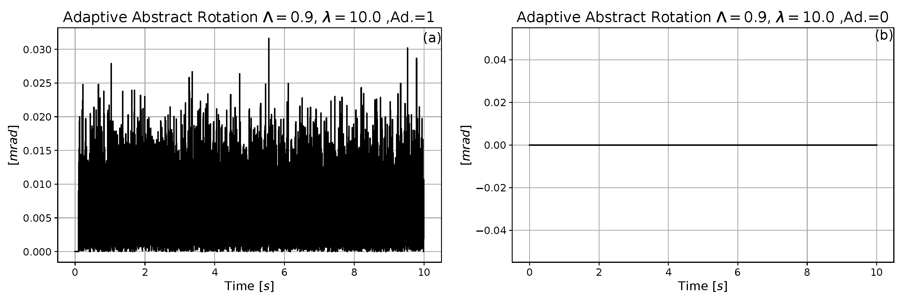
Figure 8.
The operation of the adaptive controller. (a): The desired, deformed, and realized 2nd time-derivatives. (b): The angle of the adaptive abstract rotation.
Figure 8.
The operation of the adaptive controller. (a): The desired, deformed, and realized 2nd time-derivatives. (b): The angle of the adaptive abstract rotation.

Figure 9.
The operation of the adaptive controller in the lack of measurement noises. (a): The desired, deformed, and realized 2nd time-derivatives. (b): The angle of the adaptive abstract rotation.
Figure 9.
The operation of the adaptive controller in the lack of measurement noises. (a): The desired, deformed, and realized 2nd time-derivatives. (b): The angle of the adaptive abstract rotation.

Figure 10.
Trajectory tracking for the small amplitude and high circular frequency of the nominal trajectory for which the adaptive controller was able to use only the originally learned data. (a): Non-adaptive, (b): adaptive control.
Figure 10.
Trajectory tracking for the small amplitude and high circular frequency of the nominal trajectory for which the adaptive controller was able to use only the originally learned data. (a): Non-adaptive, (b): adaptive control.

Figure 11.
Trajectory tracking error for the small amplitude and high circular frequency of the nominal trajectory for which the adaptive controller was able to use only the originally learned data. (a): Non-adaptive, (b): adaptive control.
Figure 11.
Trajectory tracking error for the small amplitude and high circular frequency of the nominal trajectory for which the adaptive controller was able to use only the originally learned data. (a): Non-adaptive, (b): adaptive control.

Figure 12.
The control torque for the small amplitude and high circular frequency of the nominal trajectory for which the adaptive controller was able to use only the originally learned data. (a): Non-adaptive, (b): adaptive control.
Figure 12.
The control torque for the small amplitude and high circular frequency of the nominal trajectory for which the adaptive controller was able to use only the originally learned data. (a): Non-adaptive, (b): adaptive control.

Figure 13.
The operation of the adaptive controller for smaller amplitude and high circular frequency of the nominal motion. (a): The desired, deformed, and realized 2nd time-derivatives. (b): The angle of the adaptive abstract rotation.
Figure 13.
The operation of the adaptive controller for smaller amplitude and high circular frequency of the nominal motion. (a): The desired, deformed, and realized 2nd time-derivatives. (b): The angle of the adaptive abstract rotation.

Figure 14.
Trajectory tracking for the small amplitude and circular frequency of the nominal trajectory. (a): Non-adaptive, (b): adaptive control.
Figure 14.
Trajectory tracking for the small amplitude and circular frequency of the nominal trajectory. (a): Non-adaptive, (b): adaptive control.

Figure 15.
Trajectory tracking error for the small amplitude and circular frequency of the nominal trajectory. (a): Non-adaptive, (b): adaptive control.
Figure 15.
Trajectory tracking error for the small amplitude and circular frequency of the nominal trajectory. (a): Non-adaptive, (b): adaptive control.

Figure 16.
The control torque for the small amplitude and circular frequency of the nominal trajectory. (a): Non-adaptive, (b): adaptive control.
Figure 16.
The control torque for the small amplitude and circular frequency of the nominal trajectory. (a): Non-adaptive, (b): adaptive control.

Figure 17.
The computational time of the control cycles. (a): Adaptive. (b): Non-adaptive.

Figure 18.
The computational time of the control cycles in ms units (zoomed in excerpts). (a): Adaptive. (b): Non-adaptive.
Figure 18.
The computational time of the control cycles in ms units (zoomed in excerpts). (a): Adaptive. (b): Non-adaptive.

Figure 19.
The trajectory tracking. (a): Adaptive. (b): Non-adaptive.

Figure 20.
The trajectory tracking error. (a): Adaptive. (b): Non-adaptive.

Figure 21.
The phase trajectory tracking. (a): Adaptive. (b): Non-adaptive.

Figure 22.
The phase trajectory of the coupled mass-point. (a): Adaptive. (b): Non-adaptive.

Figure 23.
The adaptively deformed 2nd time-derivatives. (a): Adaptive. (b): Non-adaptive.

Figure 24.
The control force. (a): Adaptive. (b): Non-adaptive.

Figure 25.
The adaptive abstract rotations. (a): Adaptive. (b): Non-adaptive.


Table 1.
The dynamic parameters of the controlled system.
| Parameter | Measurement Unit | Numerical Value |
|---|---|---|
| Inertia momentum of the wheel | ||
| Inertia of the mass-point m | ||
| Spring constant k | ||
| Spoke length r | ||
| Gravitational acceleration g | ||
| Damping constant along the spoke d |
Publisher’s Note: MDPI stays neutral with regard to jurisdictional claims in published maps and institutional affiliations. |
© 2021 by the authors. Licensee MDPI, Basel, Switzerland. This article is an open access article distributed under the terms and conditions of the Creative Commons Attribution (CC BY) license (https://creativecommons.org/licenses/by/4.0/).
Share and Cite
MDPI and ACS Style
Bitó, J.F.; Rudas, I.J.; Tar, J.K.; Varga, Á. Abstract Rotations for Uniform Adaptive Control and Soft Modeling of Mechanical Devices. Appl. Sci. 2021, 11, 7939. https://doi.org/10.3390/app11177939
AMA Style
Bitó JF, Rudas IJ, Tar JK, Varga Á. Abstract Rotations for Uniform Adaptive Control and Soft Modeling of Mechanical Devices. Applied Sciences. 2021; 11(17):7939. https://doi.org/10.3390/app11177939
Chicago/Turabian StyleBitó, János F., Imre J. Rudas, József K. Tar, and Árpád Varga. 2021. "Abstract Rotations for Uniform Adaptive Control and Soft Modeling of Mechanical Devices" Applied Sciences 11, no. 17: 7939. https://doi.org/10.3390/app11177939
Note that from the first issue of 2016, this journal uses article numbers instead of page numbers. See further details here.